ON THE WEAK-COUPLING LIMIT FOR BOSONS AND FERMIONS
31
ON THE WEAK-COUPLING LIMIT FOR BOSONS AND FERMIONS D. Benedetto * , F. Castella + , R. Esposito # and M. Pulvirenti * Abstract. In this paper we consider a large system of Bosons or Fermions. We start with an initial datum which is compatible with the Bose-Einstein, respectively Fermi-Dirac, statistics. We let the system of interacting particles evolve in a weak-coupling regime. We show that, in the limit, and up to the second order in the potential, the perturbative expansion expressing the value of the one-particle Wigner function at time t, agrees with the analogous expansion for the solution to the Uehling-Uhlenbeck equation. This paper follows in spirit the companion work [2], where the authors investigated the weak-coupling limit for particles obeying the Maxwell-Boltzmann statistics: here, they proved a (much stronger) convergence result towards the solution of the Boltzmann equation. Math. Mod. Meth. Appl. Sci., Vol. 15, N. 12, pp. 1811-1843 (2005). 1. Introduction In 1933 Uehling and Uhlenbeck in Ref. [17] proposed the following kinetic equation, called U-U in the sequel, for the time evolution of the one-particle Wigner function f (x, v; t) associated with a large system of weakly interacting Bosons or Fermions (see Ref. [18] for the definition of the Wigner function). The U-U equation is ∂ t f (x, v; t)+v ·∇ x f (x, v; t)= dv * dv * dv W (v,v * |v ,v * ) f f * (1 + 8π 3 θf )(1 + 8π 3 θf * ) - ff * (1 + 8π 3 θf )(1 + 8π 3 θf * ) , (1.1) where we use the standard short-hand notation f = f (x, v; t), f * = f (x, v * ; t), f = f (x, v ; t), f * = f (x, v * ; t). Here, W denotes the transition kernel W (v,v * |v ,v * )= 1 8π 2 φ(v - v)+ θ φ(v - v * ) 2 δ (v + v * - v - v * ) δ 1 2 (v 2 + v 2 * - v 2 - v * 2 ) . (1.2) Key words and phrases. Uehling-Uhlenbeck equation, quantum systems, weak coupling. * Dipartimento di Matematica Universit` a di Roma ‘La Sapienza’, P.le A. Moro, 5 - 00185 Roma - Italy + IRMAR, Universit´ e de Rennes 1, Campus de Beaulieu - 35042 Rennes - Cedex - France # Dipartimento di Matematica pura ed applicata, Universit` a di L’Aquila, Coppito - 67100 L’Aquila - Italy 1
Transcript of ON THE WEAK-COUPLING LIMIT FOR BOSONS AND FERMIONS

ON THE WEAK-COUPLING LIMIT FOR BOSONS AND FERMIONS
D. Benedetto∗, F. Castella+, R. Esposito# and M. Pulvirenti∗
Abstract. In this paper we consider a large system of Bosons or Fermions. We start with aninitial datum which is compatible with the Bose-Einstein, respectively Fermi-Dirac, statistics.
We let the system of interacting particles evolve in a weak-coupling regime. We show that, in
the limit, and up to the second order in the potential, the perturbative expansion expressingthe value of the one-particle Wigner function at time t, agrees with the analogous expansion
for the solution to the Uehling-Uhlenbeck equation.This paper follows in spirit the companion work [2], where the authors investigated the
weak-coupling limit for particles obeying the Maxwell-Boltzmann statistics: here, they proved
a (much stronger) convergence result towards the solution of the Boltzmann equation.
Math. Mod. Meth. Appl. Sci., Vol. 15, N. 12, pp. 1811-1843 (2005).
1. Introduction
In 1933 Uehling and Uhlenbeck in Ref. [17] proposed the following kinetic equation,called U-U in the sequel, for the time evolution of the one-particle Wigner function f(x, v; t)associated with a large system of weakly interacting Bosons or Fermions (see Ref. [18] forthe definition of the Wigner function). The U-U equation is
∂tf(x, v; t)+v · ∇xf(x, v; t) =∫
dv∗
∫dv′∗
∫dv′ W (v, v∗|v′, v′∗){
f ′f ′∗(1 + 8π3θf)(1 + 8π3θf∗)− ff∗(1 + 8π3θf ′)(1 + 8π3θf ′∗)}
,
(1.1)
where we use the standard short-hand notation
f = f(x, v; t), f∗ = f(x, v∗; t), f ′ = f(x, v′; t), f ′∗ = f(x, v′∗; t).
Here, W denotes the transition kernel
W (v, v∗|v′, v′∗) =1
8π2
[φ(v′ − v) + θ φ(v′ − v∗)
]2δ(v + v∗ − v′ − v′∗) δ
(12(v2 + v2
∗ − v′2 − v′∗2)).
(1.2)
Key words and phrases. Uehling-Uhlenbeck equation, quantum systems, weak coupling.∗ Dipartimento di Matematica Universita di Roma ‘La Sapienza’, P.le A. Moro, 5 - 00185 Roma - Italy+ IRMAR, Universite de Rennes 1, Campus de Beaulieu - 35042 Rennes - Cedex - France# Dipartimento di Matematica pura ed applicata, Universita di L’Aquila, Coppito - 67100 L’Aquila - Italy
1
2 D. BENEDETTO∗, F. CASTELLA+, R. ESPOSITO# AND M. PULVIRENTI∗
Finally,
φ(k) =∫
dx e−ik·xφ(x) (1.3)
is the Fourier transform of the two-body interaction potential φ, and θ = ±1 for Bosonsand Fermions respectively.
Note that the factors 8π3 do not appear in the original U-U equation in Ref. [17],because there, the distribution function is normalized in such a way that its integral onthe velocity variable equals the space density times 8π3. At variance, in (1.1), f is justthe standard Wigner function, whose integral on the velocities equals the space density.Let us mention that equation (1.1) actually is cubic (and not quartic) in the unknown f :apparent quartic terms have vanishing contribution, as shown by direct inspection.
Eq. (1.1) constitutes a natural modification of the usual quantum Boltzmann equation,in order to take into account statistics. In particular, there is a H-functional
H(f) =∫
dx
∫dv{f log f − θ(1 + 8π3θf) log(1 + 8π3θf)
}(1.4)
driving the system to the Bose-Einstein and Fermi-Dirac equilibrium distribution:
M(v) =1
eβµ+βv2/2 − 8π3θ(1.5)
outside the Bose condensation region. Here β and µ denote the inverse temperature andthe chemical potential respectively.
Eq. (1.1) is largely studied (see for istance [1] and [12] for physical consideration, and[15], [7], [13], [14] ... for a more mathematically oriented analysis concerning the existenceof solutions and asymptotic behavior), so that it is certainly of great relevance to derivethis equation from the first principles, namely from the Schrodinger equation.
As clearly explained by H. Spohn in [16], Eq (1.1) is indeed expected to hold in the socalled weak-coupling limit, which consists in scaling space, time and the potential accordingto
x → εx, t → εt, φ →√
εφ, (1.6)
where ε is a small positive parameter.A slightly different limit, usually called van Hove limit, scales t and φ as in (1.6) but
leaves the microscopic space scale unchanged. Eq. (1.1) cannot be derived in the van Hovelimit in general but, in case of translationally invariant states, we expect to achieve thehomogeneous version of the U-U equation (for a large system). In fact Hugenholtz [11]proved formally that this happens. Later on Ho and Landau [10] proved that the homo-geneous U-U equation holds rigorously up to the second order expansion in the potential.These approaches, as well as the recent contribution by Erdos et al. [8] (where the quantumanalog of the Boltzmann’s Stosszahlansatz is formulated), are based on the commutatorexpansion of the time evolution of the observables of the CCR and CAR algebras.
In the present paper we approach the problem from a different viewpoint. We startfrom the time evolution of a N particle quantum system in terms of the Wigner formalism.Here the statistics enters only through the choice of the admissible states we take as initialconditions. Such states, called quasi-free, must describe free Bosons and Fermions, so thatthey cannot have any other correlations but those arising from the statistics. Therefore

ON THE WEAK-COUPLING LIMIT FOR BOSONS AND FERMIONS 3
the first step is to characterize quasi-free states (see for example Ref. [4]) in terms ofthe Wigner functions. Then we apply the dynamics (in terms of the usual hierarchy) andrepresent the solution as a perturbative expansion. The truncation of this expansion upto the second order in the potential is shown to converge to the expansion associated tothe U-U equation, up to the first order in the scattering cross section.
In other words we recover the result in Ref. [10] with the following main differences.First we exploit the weak-coupling limit, so that we can deal with states which are notnecessarily translationally invariant. Second, we work directly in terms of the Wignerformalism, in the same spirit of the Balescu book (see Ref. [1]). In doing so, we alsofollow a previous work [2] by the authors for the Maxwell-Boltzmann statistics. Hence thepresent work shows how the statistics can be handled in this formalism. Note in passingthat the case of the Maxwell-Boltzmann statistics allows for a much stronger (but stillpartial) convergence result than the one presented here, see [2]. Note finally that thepresent formalism also allows to handle the low-density limit, see [3], see also the lastsection of this text.
It is also important to mention that a full rigorous derivation of the U-U equation (butalso of the usual Boltzmann equation arising for the Maxwell-Boltzmann statistics) is stillfar beyond the present techniques and those of the previous references.
The plan of the paper is the following. In the next section we describe the particlesystem. In Section 3 we establish the result. The rest of the paper is devoted to theproofs.
2. The particle system.
We consider a Quantum particle system in R3. Let
H =⊕n≥0
L2(R3)n :=⊕n≥0
Hn, (2.1)
be the Fock space. A state of the system is a self-adjoint, positive trace class operatoracting on H:
σ =⊕n≥0
σn. (2.2)
We assumeTrσ = 1. (2.3)
The operator N , number of particles, is the multiplication by n on Hn and hence
〈N〉 =∑n≥0
n Trσn, (2.4)
where the left hand side is the average number of particles in the state σ. If σn(Xn;Yn) isthe kernel of σn, the Reduced Density Matrices (RDM) are defined by:
ρn(Xn;Yn) =∑m≥0
(n + m)!m!
∫σn+m(Xn, Zm;Yn, Zm) dZm. (2.5)

4 D. BENEDETTO∗, F. CASTELLA+, R. ESPOSITO# AND M. PULVIRENTI∗
Here Xn = (x1, . . . , xn), xi ∈ R3 denotes the n-particle configuration. Note that
Tr ρn =∫
dZn ρn(Zn;Zn)
=∑m≥n
m(m− 1) . . . (m− n + 1)Trσm = 〈N(N − 1) . . . (N − n + 1)〉,(2.6)
and hence the RDM are equivalent to the classical correlation functions.The Hamiltonian of the system is the self-adjoint operator acting on H given by
H =∞⊕
n=1
Hn, (2.7)
where
Hn = −12
n∑j=1
∆xj+
∑1≤i<j≤n
φ(xi − xj), (2.8)
and the potential φ is a smooth two-body interaction. Here, ~ as well as the mass of theparticles are normalized to unity.
Under these circumstances, the time evolved state is given by the usual
σ(t) = e−iHtσeiHt. (2.9)
Now, quantum statistics is taken into account by suitable properties of the physicallyrelevant states. Namely, for the Maxwell-Boltzmann (M-B) statistics we require symmetryof ρn(x1, . . . , xn; y1 . . . , yn) in the exchange of particle names. For the Bose-Einstein (B-E)and Fermi-Dirac (F-D) statistics we require additionally
ρn(x1, . . . , xn; y1 . . . , yn) = θs(π)ρn(x1, . . . , xn; yπ(1) . . . , yπ(n)), (2.10)
where π ∈ Pn is a permutation of n elements, and s(π) = 0 if the permutation is even,s(π) = 1 if it is odd.
Alternatively, the quantum statistics is automatically taken into account by consideringstates on the algebra generated by the annihilation and creation operators a(x) and a†(x)(with the commutation and anti-commutation relations according to the B-E and F-Dstatistics respectively). Then the RDM are defined as
Tr[σa†(xn) . . . a†(x1)a(y1) . . . a(yn)
]= ρn(x1, . . . , xn; y1 . . . , yn). (2.11)
However we do not use here the second quantization formalism.Given a state σ, we define the Wigner transform [18] by
Wn(Xn;Vn) :=1
(2π)3n
∫dYn eiYn·Vnσn
(Xn −
12Yn;Xn +
12Yn
). (2.12)
Therefore the analogous of the classical correlation functions are the j-particle Wignerfunctions defined through
Fj(Xj ;Vj) =∑n≥0
(n + j)!n!
∫dXn
∫dVn Wj+n(Xj , Xn;Vj , Vn). (2.13)

ON THE WEAK-COUPLING LIMIT FOR BOSONS AND FERMIONS 5
Note that the Fj ’s are the Wigner transforms of the RDM ρj , as one can easily check.Due to the dynamics imposed by (2.9), it is a standard computation to check that the
Wigner function Wn evolves according to the Wigner-Liouville equation
∂tWn +n∑
i=1
vi · ∇xiWn = TnWn. (2.14)
As a consequence, the j-particle Wigner functions Fj ’s satisfy the associated hierarchy
∂tFj +j∑
i=1
vi · ∇xiFj = TjFj + Cj+1Fj+1, (2.15)
where Tj and Cj+1 will be defined below after Eq.(2.22), and the index j takes any valuebetween 1 and N . Equations (2.15) are analogous to the usual BBGKY hierarchy for theclassical systems and are derived in a similar manner. Note that by the definition of theRDM the coefficient in front of Cj+1 is one instead of N − j.
We now want to analyze (2.15) in the weak-coupling regime (1.6). Therefore, we set
fεj (Xj ;Vj ; t) := Fj(ε−1Xj ;Vj ; ε−1t), (2.16)
where ε > 0 is a small parameter, and we scale the potential as well, by setting
φ →√
εφ. (2.17)
The resulting, scaled, equation is
∂tfεj +
j∑i=1
vi · ∇xifε
j =1√εT ε
j fεj +
1√εε−3Cε
j+1fεj+1, (2.18)
where(T ε
j fεj )(Xj ;Vj) =
∑0<k<`≤j
(T εk,lf
εj )(Xj ;Vj), (2.19)
and the T εk,l’s are defined as follows: if j = 1, we simply have T ε
1 = 0; otherwise,
(T εk,lf
εj )(Xj ;Vj) =− i
∑σ=±1
σ
∫dh
(2π)3φ(h) ei h
ε ·(xk−x`)
fεj
(x1, . . . , xj ; v1, . . . , vk − σ
h
2, . . . , v` + σ
h
2, . . . , vj
).
(2.20)
On the other hand, the Cεj+1 in (2.18) is computed as:
(Cεj+1f
εj+1)(Xj ;Vj) =
j∑k=1
(Cεk,j+1f
εj+1)(Xj ;Vj), (2.21)
6 D. BENEDETTO∗, F. CASTELLA+, R. ESPOSITO# AND M. PULVIRENTI∗
where
(Cεk,j+1f
εj+1)(Xj ;Vj) =− i
∑σ=±1
σ
∫dh
(2π)3
∫dxj+1
∫dvj+1 φ(h) ei h
ε ·(xk−xj+1)
fεj+1
(x1, . . . , xj+1; v1, . . . , vk − σ
h
2, . . . , vj+1 + σ
h
2
).
(2.22)
Note that Tj and Cj+1 are T εj and Cε
j+1 for ε = 1. Last, we fix an initial condition sequence
{fε0,j}∞j=1 (2.23)
according to the quantum statistics, and perform the limit ε → 0 in the resulting system.
Remark: Since ∫fε0,1(x, v)dxdv = ε3〈N〉, (2.24)
requiring ‖fε0,1‖L1 = O(1), implies 〈N〉 = O(ε−3). In other words we are working in the
Grand-canonical formalism and the density is automatically rescaled.
In the following we shall fix fε0,1 to be a given (independent of ε) probability density f0.
This means that its inverse Wigner transform
ρε(x, y) =∫
dv ei x−yε ·v f0
(x + y
2, v), (2.25)
namely the one-particle rescaled RDM, is a superposition of WKB states.We now make assumptions on the initial state to take into account the statistics. For
the M-B statistics a suitable initial sequence can be chosen completely factorized, e.g.
fε0,j = f⊗j
0 . (2.26)
Such a notion of statistical independence, which corresponds to a complete factorizationof the RDM’s, is not compatible (but for the condensed Bose state) with the B-E and F-D statistics which exhibit intrinsic correlations even for non interacting particle systems.States describing free Bosons or Fermions are usually called quasi-free and are defined interms of the RDM’s by the following formula:
ρj(x1, . . . , xj ; y1, . . . , yj) =∑
π∈Pj
θs(π)
j∏i=1
ρ(xi, yπ(i)), (2.27)
for some positive definite operator ρ on L2(R3) with kernel ρ(x, y). We show in Appendixhow to construct explicitly quasi-free states for Bosons.
From now on we assume that the initial sequence (2.23) for the rescaled problem (2.18)is given by the Wigner transform of a quasi-free state (2.27) generated by ρ(x, y) = ρε(x, y)given by (2.25). As a consequence the initial sequence {f0
j }∞j=1 for the hierarchy (2.18) isof the form
f0j (Xj , Vj) =
∑π∈Pj
θs(π)fπj (Xj , Vj), (2.28)

ON THE WEAK-COUPLING LIMIT FOR BOSONS AND FERMIONS 7
with
fπj (x1, . . . , xj , v1, . . . , vj) =
1(2π)3j
∫dy1· · ·
∫dyj
∫dw1· · ·
∫dwj
j∏k=1
(eiyk·vk+iwk·
xk−xπ(k)ε −iwk·
yk+yπ(k)2 f0
(xk + xπ(k)
2− ε
4(yk − yπ(k)), wk
)).
(2.29)
Eq. (2.29) follows from (2.27) and (2.25).We underline once more that, in the present approach, the dynamics is given by the
hierarchy of equations (2.18) which are completely equivalent to the Schrodinger equation,while the statistics enters only in the structure of the initial state.
In the weak-coupling limit ε → 0, we expect that fεj (t) converges to a factorized state
(because the effects of statistics disappear in the macroscopic limit). On the more eachfactor should be solution to the U-U equation (the collisions being affected by the statisticsbecause they involve microscopic scales).
3. The main result.
Let f = f(x, v, t) be a solution to the U-U equation and set fj( · , · , t) = f⊗j( · , · , t).Then the sequence {fj}∞j=1 satisfies the following hierachy of equations:
(∂t +j∑
i=1
vi · ∇xi)fj = Qj,j+1fj+1 + Qj,j+2fj+2. (3.1)
Here the Qj,j+1 contribution, a ”two particles term” in the terminology used below, is
(Qj,j+1fj+1)(Xj , Vj) =j∑
k=1
∫dv′k
∫dvj+1
∫dv′j+1 W (vk, vj+1|v′k, v′j+1){
fj+1(Xj , xk; v1, . . . , v′k, . . . v′j+1)− fj+1(Xj , xk; v1, . . . , vj+1)
},
(3.2)
and the Qj,j+2 contribution, a ”three particles term”, is
(Qj,j+2fj+2)(Xj , Vj) = 8π3θ
j∑k=1
∫dv′k
∫dvj+1
∫dv′j+1W (vk, vj+1|v′k, v′j+1){
fj+2(Xj , xk, xk; v1, . . . , v′k, . . . v′j+1, vk) + fj+2(Xj , xk, xk; v1, . . . , v
′k, . . . v′j+1, vj+1)
− fj+2(Xj , xk xk; v1, . . . , vj+1, v′k)− fj+2(Xj xk, xk; v1, . . . , vj+1, v
′j+1)
}.
(3.3)Also, (Xn, y) denotes the (n + 1)-sequence (x1, . . . , xn, y).

8 D. BENEDETTO∗, F. CASTELLA+, R. ESPOSITO# AND M. PULVIRENTI∗
A formal solution to the hierarchy (3.1) is given by the following series expansion:
fj(t) =∑n≥0
∑α1...αnαi=1,2
∫ t
0
dt1
∫ t1
0
dt2· · ·∫ tn−1
0
dtn
S(t− t1)Qj,j+α1S(t1 − t2)Qj+α1,j+α1+α2S(t2 − t3) . . .
Qj+α1+···+αn−1,j+α1+···+αnS(tn)f⊗(j+α1+···+αn)0 ,
(3.4)
where S(t) denotes the fream stream operator, namely,
(S(t)fj)(Xj , Vj) = fj(Xj − Vjt, Vj). (3.5)
As for the solution to the ε-dependent hierarchy (2.18), we can also expand f jε in the
similar way, at least at the formal level. This gives
fεj (t) =
∑n≥0
∑γ1...γnγi=0,1
∫ t
0
dt1
∫ t1
0
dt2· · ·∫ tn−1
0
dtn
S(t− t1)P εj,j+γ1
S(t1 − t2)P εj+γ1,j+γ1+γ2
S(t2 − t3) . . .
P εj+γ1+···+γn−1,j+γ1+···+γn
S(tn)f0j+γ1+···+γn
,
(3.6)
where f0j is an initial quasi-free state given by (2.29), and
P εj,j+1 = ε−
72 Cε
j+1, P εj,j = ε−
12 T ε
j . (3.7)
We are not able to show the convergence of fεj (t) to fj(t) in the limit ε → 0 even for
short times. However we are going to show that the two series agree up to the secondorder in the potential. Namely, defining the second order contributions
g(t) := S(t)f0 +∫ t
0
dt1 S(t− t1)Q1,2S(t1)f⊗20 +
∫ t
0
dt1 S(t− t1)Q1,3S(t1)f⊗30 , (3.8)
associated with fj(t), and
gε(t) := S(t)f0 + ε−72
∫ t
0
dt1 S(t− t1)Cε2S(t1)f0
2
+ ε−4
∫ t
0
dt1
∫ t1
0
dt2 S(t− t1)Cε2S(t1 − t2)T ε
2 S(t2)f02
+ ε−7
∫ t
0
dt1
∫ t1
0
dt2 S(t− t1)Cε2S(t1 − t2)Cε
3S(t2)f03 ,
(3.9)
associated with fεj (t), we rigorously prove below the convergence of gε(t) to g(t), under
suitable assumptions on the data of the problem.
Assumptions: We require φ to be real and even, so that φ is real. In particular
φ(k) = φ(−k) = φ(−k).

ON THE WEAK-COUPLING LIMIT FOR BOSONS AND FERMIONS 9
This the most important assumption we need in the analysis. Besides, we shall need todeal with ”smooth” data. Quantitatively, we assume the following regularity:
(1 + |ξ|)α∑|β|≤2
|Dβξ φ(ξ)| ∈ L1,
for a sufficiently large α, and
f0(x, v) ∈ L1,
(1 + |ξ|+ |η|)α∑
0≤|β|≤2
∑0≤|γ|≤2
|(Dβξ + Dγ
η )f0(ξ, η)| ∈ L1, (3.10)
for a sufficiently large α as well. In (3.10), β and γ denote multi-indices, and Dβξ , Dγ
η
denote derivatives with respect to the variables ξ and η. Note that throughout this paperwe use the following normalization for the Fourier transform:
f(h) = (Fxf)(h) =∫
Rn
dx f(x) e−ih·x,
f(x) = (F−1h f)(h) =
1(2π)n
∫Rn
dh f(h) eih·x.
(3.11)
Our main result is the
Theorem. Under the above assumptions, we have
limε→0
gε(ξ, η, t) = g(ξ, η, t), for any t > 0 and any (ξ, η) ∈ R6.
Remark: In the above statement (and the proofs given below), we found convenient to treatthe terms in (3.8) and (3.9) in terms of their Fourier transforms, for which the convergencearises more naturally. However, we would like to stress that in the companion paper [2], astronger, but analogous, result is formulated in terms of the pointwise convergence in thex− v space, hence without going to the Fourier space.
Before entering the details of the proof we first analyze all the contributions in the righthand side of (3.9).
The two-particle terms are (we skip the unessential operator∫ t
0dt1 S(t− t1))
Sπ2,ε := ε−
72 Cε
2S(t1)fπ2 , (3.12)
where the permutation π may take the two values π = (1, 2) or π = (2, 1), together with
T π2,ε := ε−4
∫ t1
0
dt2 Cε2S(t1 − t2)T ε
2 S(t2)fπ2 , (3.13)
with π taking the values π = (1, 2) or π = (2, 1). There are four such terms.

10 D. BENEDETTO∗, F. CASTELLA+, R. ESPOSITO# AND M. PULVIRENTI∗
The three-particle terms are twelve, namely:
Wπ3,ε := ε−7
∫ t1
0
dt2 Cε1,2S(t1 − t2)Cε
1,3S(t2)fπ3 , (3.14)
and
Vπ3,ε := ε−7
∫ t1
0
dt2 Cε1,2S(t1 − t2)Cε
2,3S(t2)fπ3 , (3.15)
with π ∈ P3, the set of the permutations of three objects, whose cardinality is six.Note that all the above terms are funtions of (x, v) (and t1 of course).For further convenience, and in view of the proof of our main result, we readily express
all these contributions in terms of their Fourier transforms.We start with the following obvious three formulae for the basic operators S(t), T2, and
C2 (see (3.5), (2.19)-(2.20), and (2.21)-(2.22), respectively):
T ε2 f(ξ1, ξ2; η1, η2) = −i
∑σ=±1
σ
∫dh
φ(h)(2π)3
eiσ h2 ·(η2−η1)f
(ξ1 −
h
ε, ξ2 +
h
ε; η1, η2
),
Cε2 f(ξ; η) = T ε
2 f(ξ, 0; η, 0) = −i∑
σ=±1
σ
∫dh
φ(h)(2π)3
e−iσ h2 ·η f
(ξ − h
ε,h
ε; η, 0
),
S(t)f(ξ; η) = f(ξ, η + ξt).
These relations give in (3.12) through (3.15):
Sπ2,ε(ξ, η) = −i
ε−72
(2π)3∑
σ=±1
σ
∫dh φ(h) e−i σ
2 h·η fπ2
(ξ − h
ε,h
ε; η + t1(ξ −
h
ε), t1
h
ε
).
(3.16)
T π2,ε(ξ, η) =− ε−4
(2π)6∑
σ1,σ2=±1
σ1σ2
∫ t1
0
dt2
∫dh1
∫dh2 φ(h1) φ(h2)
e−iσ12 h1·η e−i
σ22 h2·(η+ξ(t1−t2)− 2
ε (t1−t2)h1)
fπ2
(ξ − 1
ε(h1 + h2),
1ε
(h1 + h2) ; η + t1ξ −t1h1 + t2h2
ε,t1h1 + t2h2
ε
),
(3.17)
Wπ3,ε(ξ, η) =− ε−7
(2π)6∑
σ1,σ2=±1
σ1σ2
∫ t1
0
dt2
∫dh1
∫dh2 φ(h1) φ(h2)
e−iσ12 h1·η e−i
σ22 h2·(η+(ξ−h1
ε )(t1−t2))
fπ3
(ξ − 1
ε(h1 + h2),
h1
ε,h2
ε; η + t1ξ −
t1h1 + t2h2
ε,t1h1
ε,t2h2
ε,
),
(3.18)
Vπ3,ε(ξ, η) =− ε−7
(2π)6∑
σ1,σ2=±1
σ1σ2
∫ t1
0
dt2
∫dh1
∫dh2 φ(h1) φ(h2)
e−iσ12 h1·η e−i
σ22 h2·
h1ε (t1−t2)
fπ3
(ξ − h1
ε,h1 − h2
ε,h2
ε; η + t1ξ −
t1h1
ε,t1h1 − t2h2
ε,t2h2
ε
).
(3.19)
ON THE WEAK-COUPLING LIMIT FOR BOSONS AND FERMIONS 11
Starting form those expressions, the plan of the proof is the following. In Section 4we evaluate the two particle terms Sπ
2,ε and T π2,ε. We prove that they converge towards
the associated two particles terms in the U-U equation. In Section 5 we deal with thethree-particle terms associated to the permutations π with a fixed element. Those areshown to converge towards the associated three particles terms in the U-U equation, whilecontributing by the quantity φ(v′−v)2 + φ(v′−v∗)2 to the transition kernel W (see (1.2)).Finally in Section 6 we treat the three particle terms relative to cyclic permutations. Werecover in this way the missing contribution to the transition kernel, namely the cross termθφ(v′ − v) φ(v′ − v∗).
For sake of simplicity we shall carry out the computations for Bosons (θ = 1), beingclear that the Fermionic case is just the same with suitable changes of sign.
4. Two-particle terms.
We introduce the partial Fourier transform
fπj (x1, . . . , xj ; η1, . . . , ηj) :=
∫dv1· · ·
∫dvj e−i
∑j
k=1vk·ηk fπ
j (x1, . . . , xj ; v1, . . . , vj).
(4.1)As a consequence of (2.29) we have
fπj (x1, . . . , xj ; η1, . . . , ηj) =
j∏k=1
f0
(xk + xπ(k)
2− ε
ηk − ηπ(k)
4,−
xk − xπ(k)
ε+
ηk + ηπ(k)
2
).
(4.2)
In particular, we have the obvious
f(1,2)2 (x1, x2; η1, η2) = f0(x1, η1)f0(x2, η2), (4.3)
together with
f(2,1)2 (x1, x2; η1, η2) =f0
(x1 + x2
2− ε
4(η1 − η2);−
x1 − x2
ε+
η1 + η2
2
)f0
(x1 + x2
2+
ε
4(η1 − η2);+
x1 − x2
ε+
η1 + η2
2
).
(4.4)
Hence, upon now performing the complete Fourier transform, we obtain,
f(1,2)2 (ξ1, ξ2; η1, η2) = f0(ξ1, η1)f0(ξ2, η2), (4.5)
together with
f(2,1)2 (ξ1, ξ2; η1, η2) =ε3
∫dy1
∫dy2 e−iξ1·(y1+
ε2 y2) e−iξ2·(y1− ε
2 y2)
f0
(y1 −
ε
4(η1 − η2);−y2 +
η1 + η2
2
)f0
(y1 +
ε
4(η1 − η2);+y2 +
η1 + η2
2
).
(4.6)

12 D. BENEDETTO∗, F. CASTELLA+, R. ESPOSITO# AND M. PULVIRENTI∗
We are now in position to analyse the term Sπ2,ε for π = (1, 2) and π = (2, 1). First,
using the identity ∑σ=±1
σe−iσ h2 ·η = −2i sin
h · η2
,
we get the the explicit expression:
Sπ2,ε = − 2ε−
72
(2π)3
∫dh φ(h) sin
(h · η2
)fπ2
(ξ − h
ε,h
ε; η + (ξ − h
ε)t1,
h
εt1
). (4.7)
In the case of S(1,2)2,ε , a change of variable h → εh then gives, using (4.5), the value
S(1,2)2,ε (ξ, η) = − 2ε−
12
(2π)3
∫dh φ(εh) sin
(εh · η2
)f0(ξ − h; η + (ξ − h)t1)f0(h, ht1). (4.8)
Therefore, we may estimate
|S(1,2)2,ε | ≤
≤ C√
ε ‖φ‖L∞
∫dh |h| (|η + (ξ − h)t1|+ |ξ − h|t1) |f0(h;ht1)| |f0|(ξ − h; η + (ξ − h)t1)
≤ C√
ε
(supξ,η
|η||f0|(ξ; η)∫
dξ supη|ξ||f0|(ξ; η) + t1 sup
ξ,η|ξ||f0|(ξ; η)
∫dξ|ξ| sup
η|f0(ξ; η)|
)
≤ C√
ε supξ,η
((|ξ|+ |η|) |f0|(ξ; η)
)∫dξ sup
η
((|ξ|+ |η|) |f0|(ξ; η)
),
(4.9)and the corresponding contribution vanishes with ε.
In the case of S(2,1)2,ε on the other hand, equations (4.7) and (4.6) give
S(2,1)2,ε (ξ, η) = − 2ε−
12
(2π)3
∫dh
∫dy1
∫dy2 φ(h) sin
(h · η2
)e−i(y1+
ε2 y2)·ξ eih·y2
f0
(y1 −
ε
4
[η + ξt1 −
2h
εt1
];−y2 +
η + ξt12
)f0
(y1 +
ε
4
[η + ξt1 −
2h
εt1
]; y2 +
η + ξt12
)= − 2ε−
12
(2π)3
∫dh
∫dy1
∫dy2 φ(h) sin
(h · η2
)e−i(y1+ε
y22 )·ξeih·y2
f0
(y1 +
h
2t1;−y2 +
η + ξt12
)f0
(y1 −
h
2t1; y2 +
η + ξt12
)+ O(
√ε).
(4.10)By the parity of φ, the first term in the right hand side is vanishing: Indeed, it is anti-symmetric in the exchange h → −h and y2 → −y2. Note that the mechanism that makesthe dominant, O(ε−1/2), contribution of S(2,1)
2,ε , vanish in the limit, is very different from
the one involved in the vanishing of S(1,2)2,ε : here, antisymmetry plays a crucial role. This
aspect will play an even more important, and more intricate, role in the next two sections.

ON THE WEAK-COUPLING LIMIT FOR BOSONS AND FERMIONS 13
There remains to prove that the O(√
ε) term in (4.10) indeed has the claimed size. It canbe written as
− 2ε12
(2π)6
∫dh dy2 dξ1 φ(h) sin
(h · η2
)f0
(ξ1;
η + ξt12
− y2
)f0
(ξ − ξ1;
η + ξt12
+ y2
)eih·y2+i
t12 h·(2ξ1−ξ)
(1− ei ε
2
(−y2·ξ+(ξ−2ξ1)·
(η+ξt1
2
))).
It may be estimated by
Cε12
∫dh |φ|(h)
∫dy2 dξ1 |f0|
(ξ1;
η + ξt12
+ y2
)|f0|
(ξ − ξ1;
η + ξt12
− y2
)(|ξ1|
∣∣∣∣η + ξt12
+ y2
∣∣∣∣+ |ξ − ξ1|∣∣∣∣η + ξt1
2− y2
∣∣∣∣) .
Therefore the term S(2,1)2,ε vanishes as well.
As a conclusion, all terms Sπ2,ε, which are the ones that are linear in φ, vanish in the
limit ε → 0.
We now pass to the evaluation of the terms T π2,ε.
The contribution T (1,2)2,ε has been already considered in Ref. [2]. However, for sake of
completeness, we analyze this term in the present context as well. Using (4.5) in (3.17),and performing the change of variables:
h1 + h2
ε= k, h2 = h,
t1 − t2ε
= s, (4.11)
we arrive at
T (1,2)2,ε (ξ, η) = − 1
(2π)6∑
σ1,σ2=±1
σ1σ2
∫ t1ε
0
ds
∫dh
∫dk φ(h)φ(−h + εk)
e−i[η·h(σ2−σ12 )+σ2h2s] e−iε
σ12 k·η e−iεσ2
h2 ·[ξs−2sk]
f0(ξ − k; η + t1ξ + hs− kt1) f0(k; kt1 − hs).
(4.12)
This term converges formally to
T (1,2)2 (ξ, η) = − 1
(2π)6∑
σ1,σ2=±1
σ1σ2
∫ +∞
0
ds
∫dh
∫dk |φ(h)|2
e−i[η·h(σ2−σ12 )+σ2h2s] f0(ξ − k; η + t1ξ + hs− kt1) f0(k; kt1 − hs).
(4.13)
To justify the limit we split the integration in ds over the two intervals [0, 1], [1,+∞]. Inthe first interval we bound the integrand by
‖φ‖L∞ ‖f0‖L∞ |φ(h)| supη|f0(k, η)|, (4.14)
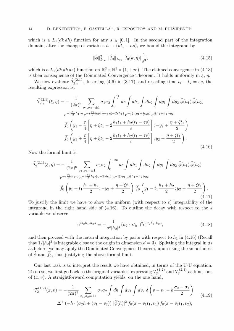
14 D. BENEDETTO∗, F. CASTELLA+, R. ESPOSITO# AND M. PULVIRENTI∗
which is a L1(dk dh) function for any s ∈ [0, 1]. In the second part of the integrationdomain, after the change of variables h → (kt1 − hs), we bound the integrand by
‖φ‖2L∞ ‖f0‖L∞ |f0(k, η)| 1s3
, (4.15)
which is a L1(dk dh ds) function on R3×R3× (1,+∞). The claimed convergence in (4.13)is then consequence of the Dominated Convergence Theorem. It holds uniformly in ξ, η.
We now evaluate T (2,1)2,ε . Inserting (4.6) in (3.17), and rescaling time t1 − t2 = εs, the
resulting expression is:
T (2,1)2,ε (ξ, η) =− 1
(2π)6∑
σ1,σ2=±1
σ1σ2
∫ t1ε
0
ds
∫dh1
∫dh2
∫dy1
∫dy2 φ(h1) φ(h2)
e−iσ12 h1·η e−i
σ22 h2·(η+εsξ−2sh1) e−iξ·(y1+
ε2 y2) ei(h1+h2)·y2
f0
(y1 −
ε
4
[η + ξt1 − 2
h1t1 + h2(t1 − εs)ε
];−y2 +
η + ξt12
)f0
(y1 +
ε
4
[η + ξt1 − 2
h1t1 + h2(t1 − εs)ε
]; y2 +
η + ξt12
).
(4.16)Now the formal limit is:
T (2,1)2 (ξ, η) =− 1
(2π)6∑
σ1,σ2=±1
σ1σ2
∫ +∞
0
ds
∫dh1
∫dh2
∫dy1
∫dy2 φ(h1) φ(h2)
e−iσ12 h1·η e−i
σ22 h2·(η−2sh1) e−iξ·y1 ei(h1+h2)·y2
f0
(y1 + t1
h1 + h2
2;−y2 +
η + ξt12
)f0
(y1 − t1
h1 + h2
2; y2 +
η + ξt12
).
(4.17)To justify the limit we have to show the uniform (with respect to ε) integrability of theintegrand in the right hand side of (4.16). To outline the decay with respect to the svariable we observe
eiσ2h1·h2s = − 1s2|h2|4
(h2 · ∇h1)2eiσ2h1·h2s, (4.18)
and then proceed with the natural integration by parts with respect to h1 in (4.16) (Recallthat 1/|h2|2 is integrable close to the origin in dimension d = 3). Splitting the integral in dsas before, we may apply the Dominated Convergence Theorem, upon using the smoothnessof φ and f0, thus justifying the above formal limit.
Our last task is to interpret the result we have obtained, in terms of the U-U equation.To do so, we first go back to the original variables, expressing T (1,2)
2 and T (2,1)2 as functions
of (x, v). A straightforward computation yields, on the one hand,
T (1,2)2 (x, v) = − 1
(2π)3∑
σ1,σ2=±1
σ1σ2
∫dh
∫dv1
∫dv2 δ
(v − v1 − h
σ2 − σ1
2
)∆+ (−h · (σ2h + (v1 − v2)) |φ(h)|2 f0(x− v1t1, v1) f0(x− v2t1, v2),
(4.19)
ON THE WEAK-COUPLING LIMIT FOR BOSONS AND FERMIONS 15
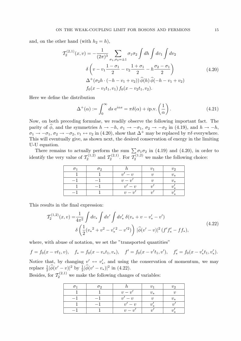
and, on the other hand (with h2 = h),
T (2,1)2 (x, v) = − 1
(2π)3∑
σ1,σ2=±1
σ1σ2
∫dh
∫dv1
∫dv2
δ
(v − v1
1− σ1
2− v2
1 + σ1
2− h
σ2 − σ1
2
)∆+(σ2h · (−h− v1 + v2)) φ(h) φ(−h− v1 + v2)
f0(x− v1t1, v1) f0(x− v2t1, v2).
(4.20)
Here we define the distribution
∆+(α) :=∫ ∞
0
ds eiαs = πδ(α) + ip.v.(
1α
). (4.21)
Now, on both preceding formulae, we readily observe the following important fact. Theparity of φ, and the symmetries h → −h, σ1 → −σ1, σ2 → −σ2 in (4.19), and h → −h,σ1 → −σ1, σ2 → −σ2, v1 ↔ v2 in (4.20), show that ∆+ may be replaced by πδ everywhere.This will eventually give, as shown next, the desired conservation of energy in the limitingU-U equation.
There remains to actually perform the sum∑
σ1σ2 in (4.19) and (4.20), in order toidentify the very value of T (1,2)
2 and T (2,1)2 . For T (1,2)
2 we make the following choice:
σ1 σ2 h v1 v2
1 1 v′ − v v v∗−1 −1 v − v′ v v∗
1 −1 v′ − v v′ v′∗−1 1 v − v′ v′ v′∗
This results in the final expression:
T (1,2)2 (x, v) =
14π2
∫dv∗
∫dv′∫
dv′∗ δ(v∗ + v − v′∗ − v′)
δ
(12(v∗2 + v2 − v′∗
2 − v′2))|φ(v′ − v)|2 (f ′f ′∗ − ff∗),
(4.22)
where, with abuse of notation, we set the ”transported quantities”
f = f0(x− vt1, v), f∗ = f0(x− v∗t1, v∗), f ′ = f0(x− v′t1, v′), f ′∗ = f0(x− v′∗t1, v
′∗).
Notice that, by changing v′ ↔ v′∗, and using the conservation of momentum, we mayreplace 1
2 |φ(v′ − v)|2 by 12 |φ(v′ − v∗)|2 in (4.22).
Besides, for T (2,1)2 we make the following changes of variables:
σ1 σ2 h v1 v2
1 1 v − v′ v∗ v−1 −1 v′ − v v v∗
1 −1 v′ − v v′∗ v′
−1 1 v − v′ v′ v′∗

16 D. BENEDETTO∗, F. CASTELLA+, R. ESPOSITO# AND M. PULVIRENTI∗
This results in the final expression:
T (2,1)2 (x, v) =
14π2
∫dv∗
∫dv′∫
dv′∗ δ(v∗ + v − v′∗ − v′)
δ
(12(v∗2 + v2 − v′∗
2 − v′2))
φ(v′ − v) φ(v′ − v∗) (f ′f ′∗ − ff∗).(4.23)
As a conclusion for the T2 terms, we have eventually established the (desired) equality
T (1,2)2 + T (2,1)
2 =∫
dv∗
∫dv′∫
dv∗W (v, v∗|v′, v′∗)(f ′f ′∗ − ff∗). (4.24)
This ends up the analysis of the two-particle terms.
5. Three-particle terms: permutations with a fixed element
In this section we analyze Wπ3,ε and Vπ
3,ε for the permutations π with a fixed element.To simplify the notation we set
W03,ε and V0
3,ε for π = (1, 2, 3),
andWi
3,ε and Vi3,ε, i = 1, 2, 3,
for the three permutations leaving i fixed. To state the result briefly, let us readily saythat the factors
W03,ε, V0
3,ε, together with W23,ε, V1
3,ε,
give a vanishing contribution. Also, the sum
W33,ε + V3
3,ε
is shown to vanish asymptotically, while each of these two terms is O(ε−1) separately.Here, anti-symmetry will play a central role. Finally, the two terms
W13,ε, V2
3,ε,
do contribute to the limiting U-U equation through the cubic term. They build up thetransition kernel φ(v′ − v)2 + φ(v′ − v∗)2. The missing cross term 2φ(v′ − v) φ(v′ − v∗) inW (v, v∗|v′, v′∗) will come up in the next section.
Let us show first that W03,ε and V0
3,ε are vanishing. From (3.18), scaling h1 and h2 andsumming on σ1, σ2, we have
W03,ε = +4
ε−1
(2π)6
∫ t1
0
dt2
∫dh1
∫dh2 φ(εh1) φ(εh2)
sin(
εh1 · η
2
)sin(
εh2
2· (η + (t1 − t2)(ξ − h1)
)f0(ξ − (h1 + h2), η + t1ξ − (t1h1 + t2h2)) f0(h1, t1h1) f0(h2, t2h2)
= O(ε),
(5.1)

ON THE WEAK-COUPLING LIMIT FOR BOSONS AND FERMIONS 17
due to the decay properties of f0. The same argument easily leads to V03,ε = O(ε).
We now pass to the computation of W13,ε. This term is associated with the permutation
π = (1, 3, 2). Upon Fourier transforming in x the relation (4.2) for fπj (with j = 3), and
using the change of variables y1 = (x2 + x3)/2, y2 = (x2 − x3)/ε in the correspondingformula, we recover
f(1,3,2)3,ε (ξ1,ξ2, ξ3, η1, η2, η3) = ε3f0(ξ1, η1)
∫dy1
∫dy2 e−iξ2·(y1+
ε2 y2) e−iξ3·(y1− ε
2 y2)
f0
(y1 − ε
η2 − η3
4,−y2 +
η2 + η3
2
)f0
(y1 + ε
η2 − η3
4, y2 +
η2 + η3
2
).
(5.2)
Then, inserting (5.2) in the formula (3.18) relating the value of Wπ3,ε, we arrive at
W13,ε(ξ, η) = − ε−4
(2π)6∑
σ1,σ2=±1
σ1σ2
∫ t1
0
dt2
∫dh1
∫dh2
∫dy1
∫dy2 φ(h1) φ(h2)
e−i(
h1+h2ε ·y1+
h1−h22 ·y2
)e−i
σ12 h1·η e−i
σ22 h2·
(η+(t1−t2)(ξ−
h1ε ))
f0
(ξ − h1 + h2
ε, η + t1ξ −
t1h1 + t2h2
ε
)f0
(y1 −
t1h1 − t2h2
4,t1h1 + t2h2
2ε− y2
)f0
(y1 +
t1h1 − t2h2
4,t1h1 + t2h2
2ε+ y2
).
(5.3)
Changing variables
k =h1 + h2
ε, h = h2, s =
t1 − t2ε
,
we obtain
W13,ε(ξ, η) = − 1
(2π)6∑
σ1,σ2=±1
σ1σ2
∫ t1ε
0
ds
∫dh
∫dk
∫dy1
∫dy2 φ(−h + εk) φ(h)
e−iσ12 η·(−h+εk) e−i
σ22 h·(η+sh+εs(ξ−k)) e−ik·y1−iy2(−h+ε k
2 ) f0(ξ − k, η + t1(ξ − k) + sh)
f0
(y1 +
t1h
2− ε
kt1 + sh
4,kt1 − sh
2− y2
)f0
(y1 −
t1h
2+ ε
kt1 + sh
4,kt1 − sh
2+ y2
).
(5.4)We are now in position to identify the rigorous limit of W1
3,ε, using the assumed decay ofφ and f0. The argument are those used in the previous section: we do not repeat themhere and in the sequel. Passing to the limit we get, eventually,
W13(ξ, η) = − 1
(2π)6∑
σ1,σ2=±1
σ1σ2
∫ +∞
0
ds
∫dh
∫dk
∫dy1
∫dy2 |φ(h)|2
eiσ1−σ2
2 h·ηe−iσ22 h2s e−ik·y1+ih·y2 f0(ξ − k, η + t1(ξ − k) + sh)
f0
(y1 +
t1h
2,kt1 − sh
2− y2
)f0
(y1 −
t1h
2,kt1 − sh
2+ y2
).
(5.5)

18 D. BENEDETTO∗, F. CASTELLA+, R. ESPOSITO# AND M. PULVIRENTI∗
Last, we go back to the (x, v) variables, computing the inverse Fourier transform of theabove term. This gives
W13 (x, v) = −π
∑σ1,σ2=±1
σ1σ2
∫dv1
∫dv2
∫dv3 |φ(v2 − v3)|2
δ
([v2 − v3] ·
[−v + v2
1 + σ1
2+ v3
1− σ1
2
])δ
(v − v1 +
σ1 − σ2
2(v3 − v2)
)f0(x− v1t1, v1) f0(x− v2t1, v2) f0(x− v3t1, v3).
(5.6)This is our final expression of W1
3 . It will be interpreted later in terms of the v, v∗, v′, v′∗variables of the U-U equation.
In a similar fashion we compute V23,ε and its limit V2
3 . We write
f(3,2,1)3,ε (ξ1,ξ2, ξ3, η1, η2, η3) = ε3f0(ξ2, η2)
∫dy1
∫dy2 e−iξ1·(y1+
ε2 y2) e−iξ3·(y1− ε
2 y2)
f0
(y1 − ε
η1 − η3
4,−y2 +
η2 + η1
2
)f0
(y1 + ε
η1 − η3
4, y2 +
η1 + η3
2
).
(5.7)
We insert this expression into (3.19), and perform the change of variables h = h2, k =(h1 − h2)/ε, and s = (t1 − t2)/ε. Passing to the limit ε → 0 at once, gives the asymptoticvalue
V23 (ξ, η) = − 1
(2π)6∑
σ1,σ2=±1
σ1σ2
∫ +∞
0
ds
∫dh
∫dk
∫dy1
∫dy2 |φ(h)|2
f0
(y1 +
t1h
2,η + ξt1 − kt1 − sh
2− y2
)f0
(y1 −
t1h
2,η + ξt1 − kt1 − sh
2+ y2
)f0(k, t1k + sh) e−i(ξ−k)·y1 eih·y2e−i
σ12 h·η e−i
σ22 h2s,
(5.8)whose inverse Fourier transform is
V23 (x, v) = −π
∑σ1,σ2=±1
σ1σ2
∫dv1
∫dv2
∫dv3 |φ(v1 − v3)|2
δ
([v1 − v3] ·
[v2 − v1
1 + σ2
2− v3
1− σ2
2
])δ
(v − v1
1− σ1
2− v3
1 + σ1
2
)f0(x− v1t1, v1)f0(x− v2t1, v2) f0(x− v3t1, v3).
(5.9)
Before coming to the computation of the other Wi3’s and Vi
3’s, let us now identify thelink between the obtained values of W1
3 , V23 , and the U-U equation. The following changes
of variables in W13
σ1 σ2 v1 v2 v3
1 1 v v′∗ v∗−1 −1 v v∗ v′∗
1 −1 v′ v′∗ v∗−1 1 v′ v∗ v′∗
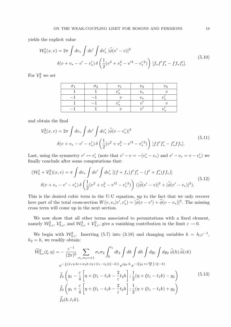
ON THE WEAK-COUPLING LIMIT FOR BOSONS AND FERMIONS 19
yields the explicit value
W13 (x, v) = 2π
∫dv∗
∫dv′∫
dv′∗ |φ(v′ − v)|2
δ(v + v∗ − v′ − v′∗) δ
(12(v2 + v2
∗ − v′2 − v′∗2))
[f∗f ′f ′∗ − ff∗f′∗].
(5.10)
For V23 we set
σ1 σ2 v1 v2 v3
1 1 v′∗ v∗ v−1 −1 v v∗ v′∗
1 −1 v′∗ v′ v−1 1 v v′ v′∗
and obtain the final
V23 (x, v) = 2π
∫dv∗
∫dv′∫
dv′∗ |φ(v − v′∗)|2
δ(v + v∗ − v′ − v′∗) δ
(12(v2 + v2
∗ − v′2 − v′∗2))
[ff ′f ′∗ − f ′∗ff∗].(5.11)
Last, using the symmetry v′ ↔ v′∗ (note that v′ − v = −(v′∗ − v∗) and v′ − v∗ = v− v′∗) wefinally conclude after some computations that:
(W13 + V2
3 )(x, v) = π
∫dv∗
∫dv′∫
dv′∗ [(f + f∗)f ′f ′∗ − (f ′ + f ′∗)ff∗)]
δ(v + v∗ − v′ − v′∗) δ
(12(v2 + v2
∗ − v′2 − v′∗2))
(|φ(v′ − v)|2 + |φ(v′ − v∗)|2).(5.12)
This is the desired cubic term in the U-U equation, up to the fact that we only recoverhere part of the total cross-section W (v, v∗|v′, v′∗) = [φ(v − v′) + φ(v − v∗)]2. The missingcross term will come up in the next section.
We now show that all other terms associated to permutations with a fixed element,namely W2
3,ε, V13,ε, and W3
3,ε + V33,ε, give a vanishing contribution in the limit ε → 0.
We begin with W23,ε. Inserting (5.7) into (3.18) and changing variables k = h1ε
−1,h2 = h, we readily obtain:
W23,ε(ξ, η) =− ε−1
(2π)6∑
σ1,σ2=±1
σ1σ2
∫ t1
0
dt2
∫dk
∫dh
∫dy1
∫dy2 φ(h) φ(εk)
e−i2 (σ1η·kε+σ2h·(η+(t1−t2)(ξ−k)) eiy2·h e−i(y1+ε
y22 )·(ξ−k)
f0
(y1 −
ε
4
[η + ξt1 − t1k −
2εt2h
];12(η + ξt1 − t1k)− y2
)f0
(y1 +
ε
4
[η + ξt1 − t1k −
2εt2h
];12(η + ξt1 − t1k) + y2
)f0(k, t1k).
(5.13)
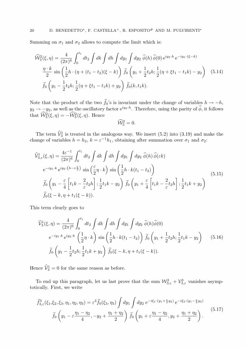
20 D. BENEDETTO∗, F. CASTELLA+, R. ESPOSITO# AND M. PULVIRENTI∗
Summing on σ1 and σ2 allows to compute the limit which is:
W23 (ξ, η) =
4(2π)6
∫ t1
0
dt2
∫dk
∫dh
∫dy1
∫dy2 φ(h) φ(0) eiy2·h e−iy1·(ξ−k)
η · k2
sin(
12h · (η + (t1 − t2)(ξ − k)
)f0
(y1 +
12t2h;
12(η + ξt1 − t1k)− y2
)f0
(y1 −
12t2h;
12(η + ξt1 − t1k) + y2
)f0(k, t1k).
(5.14)
Note that the product of the two f0’s is invariant under the change of variables h → −h,y2 → −y2, as well as the oscillatory factor eiy2·h. Therefore, using the parity of φ, it followsthat W2
3 (ξ, η) = −W23 (ξ, η). Hence
W23 = 0.
The term V13 is treated in the analogous way. We insert (5.2) into (3.19) and make the
change of variables h = h2, k = ε−1h1, obtaining after summation over σ1 and σ2:
V13,ε(ξ, η) =
4ε−1
(2π)6
∫ t1
0
dt2
∫dk
∫dh
∫dy1
∫dy2 φ(h) φ(εk)
e−iy1·k eiy2·(h−ε k2 ) sin
(ε
2η · k
)sin(
12h · k(t1 − t2)
)f0
(y1 −
ε
4
[t1k −
2εt2h
];12t1k − y2
)f0
(y1 +
ε
4
[t1k −
2εt2h
];12t1k + y2
)f0(ξ − k, η + t1(ξ − k)).
(5.15)
This term clearly goes to
V13 (ξ, η) =
4(2π)6
∫ t1
0
dt2
∫dk
∫dh
∫dy1
∫dy2 φ(h)φ(0)
e−iy1·k eiy2·h(
12η · k
)sin(
12h · k(t1 − t2)
)f0
(y1 +
12t2h;
12t1k − y2
)f0
(y1 −
12t2h;
12t1k + y2
)f0(ξ − k, η + t1(ξ − k)).
(5.16)
Hence V13 = 0 for the same reason as before.
To end up this paragraph, let us last prove that the sum W33,ε + V3
3,ε vanishes asymp-totically. First, we write
f33,ε(ξ1,ξ2, ξ3, η1, η2, η3) = ε3f0(ξ3, η3)
∫dy1
∫dy2 e−iξ1·(y1+
ε2 y2) e−iξ2·(y1− ε
2 y2)
f0
(y1 − ε
η1 − η2
4,−y2 +
η1 + η2
2
)f0
(y1 + ε
η1 − η2
4, y2 +
η1 + η2
2
).
(5.17)

ON THE WEAK-COUPLING LIMIT FOR BOSONS AND FERMIONS 21
We insert this formmula in (3.18), and perform the change of variables h1 = h, h2 = εk.In this way we recover, upon computing the sum
∑σ1σ2,
W33,ε(ξ, η) =
4ε−1
(2π)6
∫ t1
0
dt2
∫dk
∫dh
∫dy1
∫dy2 φ(h) φ(εk)
eiy2·h e−i(y1+ε2 y2)·(ξ−k) sin
(12η · h
)sin(
εk
2· (η + (t1 − t2)ξ)−
12k · h(t1 − t2)
)f0
(y1 −
ε
4
[η + ξt1 − kt2 −
2εt1h
];12(h + ξt1 − t2k)− y2
)f0
(y1 +
ε
4
[η + ξt1 − kt2 −
2εt1h
];12(η + ξt1 − t2k) + y2
)f0(k, t2k).
(5.18)Similarly, using (5.17), (3.19), and performing again the change of variables h1 = h,h2 = εk, we obtain:
V33,ε(ξ, η) =
4ε−1
(2π)6
∫ t1
0
dt2
∫dk
∫dh
∫dy1
∫dy2 φ(h) φ(εk)
eiy2·h e−iy1·(ξ−k) e−i ε2 y2·(ξ+k)
sin(
12η · h
)sin(
12k · h(t1 − t2)
)f0
(y1 +
ε
4
[η + ξt1 + kt2 −
2εt1h
];12(η + ξt1 − t2k) + y2
)f0
(y1 −
ε
4
[η + ξt1 + kt2 −
2εt1h
];12(η + ξt1 − t2k)− y2
)f0(k, t2k).
(5.19)
Hence, both terms W33,ε and V3
3,ε are O(ε−1). However we have the following expansions:
εW33,ε = A0 + εA1 + O(ε2), εV3
3,ε = B0 + εB1 + O(ε2),
and it is easy to realize that A0 = −B0. Moreover, after some straightforward calculation,we obtain at the next order:
A1 + B1 =4ε−1
(2π)6
∫ t1
0
dt2
∫dk
∫dh
∫dy1
∫dy2 φ(h) φ(0)eiy2·h e−iy1·(ξ−k) sin
(12η · h
)f0(k, t2k)f0
(y1 −
12t1h;
12(η + ξt1 − t2k) + y2
)f0
(y1 +
12t1h;
12(η + ξt1 − t2k)− y2
){
k
2· (η + (t1 − t2)ξ) cos
(12k · h(t1 − t2)
)+
sin(
12k · h(t1 − t2)
) (12t2k · ∇x log
f0((y1 − 12 t1h; 1
2 (η + ξt1 − t2k) + y2)
f0((y1 + 12 t1h; 1
2 (η + ξt1 − t2k)− y2)− iy2 · k
)}.
(5.20)

22 D. BENEDETTO∗, F. CASTELLA+, R. ESPOSITO# AND M. PULVIRENTI∗
Let us now exchange h → −h and y2 → −y2. The term in braces is invariant because thelog term changes its sign. All the other terms are invariant but sin(η ·h/2), which changessign. Therefore A1 + B1 = −(A1 + B1), hence A1 + B1 = 0. This shows that W3
3,ε + V33,ε
vanishes in the limit ε → 0.
6. Three-particle terms: cyclic permutations
We still have to evaluate Wπ3,ε, Wπ−1
3,ε , Vπ3,ε and Vπ−1
3,ε with π = (2, 3, 1) and π−1 =(3, 1, 2).
We first observe, for later convenience, the two relations
fπ−1
3 (ξ1, ξ2, ξ3;η1, η2, η3) =∫
dx1
∫dx2
∫dx3 e−i
∑3
k=1xk·ξk
f0
(x1 + x2
2+
ε
4(η1 − η2);
x1 − x2
ε+
η1 + η2
2
)f0
(x2 + x3
2+
ε
4(η2 − η3);
x2 − x3
ε+
η2 + η3
2
)f0
(x3 + x1
2+
ε
4(η3 − η1);
x3 − x1
ε+
η3 + η1
2
),
(6.1)
fπ3 (ξ1, ξ2, ξ3;η1, η2, η3) =
∫dx1
∫dx2
∫dx3 e−i
∑3
k=1xk·ξk
f0
(x2 + x1
2+
ε
4(η2 − η1);
x2 − x1
ε+
η2 + η1
2
)f0
(x3 + x2
2+
ε
4(η3 − η2);
x3 − x2
ε+
η3 + η2
2
)f0
(x1 + x3
2+
ε
4(η1 − η3);
x1 − x3
ε+
η1 + η3
2
).
(6.2)
Armed with these expressions, we begin with the computation of Wπ−1
3,ε and Wπ3,ε. To do
so, we insert (6.1) and (6.2) in the general formula (3.18) relating the value of the Wπ3,ε’s.
In the so-obtained formulae, we also change variables, h1 → −h1, h2 → −h2 for π−1, andσ1 → −σ1, σ2 → −σ2 for π. With this new set of variables, the ξ’s and η’s involved in(3.18) are
ξ1 = ξ ± h1 + h2
ε, ξ2 = ∓h1
ε, ξ3 = ∓h2
ε,
η1 = η + ξt1 ±t1h1 + t2h2
ε, η2 = ∓ t1h1
ε, η3 = ∓ t2h2
ε,
(6.3)
for π−1 and π respectively. Also, the phases appearing in (3.18) are:
Sπ−1 =σ1
2h1 · η +
σ2
2h2
(η + (t1 − t2)
[ξ +
h1
ε
]),
Sπ =σ1
2h1 · η +
σ2
2h2
(η + (t1 − t2)
[ξ − h1
ε
]).
(6.4)
ON THE WEAK-COUPLING LIMIT FOR BOSONS AND FERMIONS 23
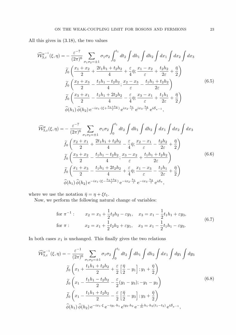
All this gives in (3.18), the two values
Wπ−1
3,ε (ξ, η) =− ε−7
(2π)6∑
σ1σ2=±1
σ1σ2
∫ t1
0
dt2
∫dh1
∫dh2
∫dx1
∫dx2
∫dx3
f0
(x1 + x2
2+
2t1h1 + t2h2
4+
ε
4η;
x1 − x2
ε+
t2h2
2ε+
η
2
)f0
(x2 + x3
2− t1h1 − t2h2
4;x2 − x3
ε− t1h1 + t2h2
2ε
)f0
(x3 + x1
2− t1h1 + 2t2h2
4− ε
4η;
x3 − x1
ε+
t1h1
2ε+
η
2
)φ(h1) φ(h2) e−ix1·(ξ+
h1+h2ε ) eix2·
h1ε eix3·
h2ε eiSπ−1 ,
(6.5)
Wπ3,ε(ξ, η) =− ε−7
(2π)6∑
σ1σ2=±1
σ1σ2
∫ t1
0
dt2
∫dh1
∫dh2
∫dx1
∫dx2
∫dx3
f0
(x2 + x1
2+
2t1h1 + t2h2
4− ε
4η;
x2 − x1
ε− t2h2
2ε+
η
2
)f0
(x3 + x2
2− t1h1 − t2h2
4;x3 − x2
ε+
t1h1 + t2h2
2ε
)f0
(x1 + x3
2− t1h1 + 2t2h2
4+
ε
4η;
x1 − x3
ε− t1h1
2ε+
η
2
)φ(h1) φ(h2) e−ix1·(ξ−
h1+h2ε ) e−ix2·
h1ε e−ix3·
h2ε eiSπ ,
(6.6)
where we use the notation η = η + ξt1.Now, we perform the following natural change of variables:
for π−1 : x2 = x1 +12t2h2 − εy1, x3 = x1 −
12t1h1 + εy3,
for π : x2 = x1 +12t2h2 + εy1, x3 = x1 −
12t1h1 − εy3.
(6.7)
In both cases x1 is unchanged. This finally gives the two relations
Wπ−1
3,ε (ξ, η) =− ε−1
(2π)6∑
σ1σ2=±1
σ1σ2
∫ t1
0
dt2
∫dh1
∫dh2
∫dx1
∫dy1
∫dy3
f0
(x1 +
t1h1 + t2h2
2+
ε
2
[ η2− y1
]; y1 +
η
2
)f0
(x1 −
t1h1 − t2h2
2− ε
2(y1 − y3);−y1 − y3
)f0
(x1 −
t1h1 + t2h2
2− ε
2
[ η2− y3
]; y3 +
η
2
)φ(h1) φ(h2) e−ix1·ξ e−iy1·h1 eiy3·h2 e−
i2ε h1·h2(t1−t2) eiSπ−1 ,
(6.8)

24 D. BENEDETTO∗, F. CASTELLA+, R. ESPOSITO# AND M. PULVIRENTI∗
Wπ3,ε(ξ, η) =− ε−1
(2π)6∑
σ1σ2=±1
σ1σ2
∫ t1
0
dt2
∫dh1
∫dh2
∫dx1
∫dy1
∫dy3
f0
(x1 +
t1h1 + t2h2
2− ε
2
[ η2− y1
]; y1 +
η
2
)f0
(x1 −
t1h1 − t2h2
2+
ε
2(y1 − y3);−y1 − y3
)f0
(x1 −
t1h1 + t2h2
2+
ε
2
[ η2− y3
]; y3 +
η
2
)φ(h1) φ(h2) e−ix1·ξ e−iy1·h1 eiy3·h2 e
i2ε h1·h2(t1−t2) eiSπ .
(6.9)
Next, we come to the computation of Vπ3,ε and Vπ−1
3,ε . We insert (6.1) and (6.2) in (3.19).We also change h1 → −h1, σ2 → −σ2 for π−1 and h2 → −h2, σ2 → −σ2 for π. This givesthe two identities
Vπ−1
3,ε (ξ, η) =− ε−7
(2π)6∑
σ1σ2=±1
σ1σ2
∫ t1
0
dt2
∫dh1
∫dh2
∫dx1
∫dx2
∫dx3
f0
(x1 + x2
2+
2t1h1 + t2h2
4+
ε
4η;
x1 − x2
ε− t2h2
2ε+
η
2
)f0
(x3 + x1
2− t1h1 − t2h2
4− ε
4η;
x3 − x1
ε+
t1h1 + t2h2
2ε+
η
2
)f0
(x2 + x3
2− t1h1 + 2t2h2
4;x2 − x3
ε− t1h1
2ε
)φ(h1) φ(h2) e−ix1·(ξ+
h1ε ) eix2·
h1+h2ε e−ix3·
h2ε eiSπ−1 ,
(6.10)
Vπ3,ε(ξ, η) =− ε−7
(2π)6∑
σ1σ2=±1
σ1σ2
∫ t1
0
dt2
∫dh1
∫dh2
∫dx1
∫dx2
∫dx3
f0
(x2 + x1
2+
2t1h1 + t2h2
4− ε
4η;
x2 − x1
ε+
t2h2
2ε+
η
2
)f0
(x1 + x3
2− t1h1 − t2h2
4+
ε
4η;
x1 − x3
ε− t1h1 + t2h2
2ε+
η
2
)f0
(x3 + x2
2− t1h1 + 2t2h2
4;x3 − x2
ε+
t1h1
2ε
)φ(h1) φ(h2) e−ix1·(ξ−
h1ε ) e−ix2·
h1+h2ε eix3·
h2ε eiSπ .
(6.11)
Here the phases are:
Sπ−1 =σ1
2h1 · η +
σ2
2h2 ·
h1
ε(t1 − t2),
Sπ =σ1
2h1 · η −
σ2
2h2 ·
h1
ε(t1 − t2).
(6.12)

ON THE WEAK-COUPLING LIMIT FOR BOSONS AND FERMIONS 25
We make the following natural change of variable
for π−1 : x1 = x′1 +12t2h2, x2 = x′1 − εy1, x3 = x′1 −
12t1h1 − ε
(y1 + y3 +
η
2
),
for π : x1 = x′1 +12t2h2, x2 = x′1 + εy1, x3 = x′1 −
12t1h1 + ε
(y1 + y3 +
η
2
).
(6.13)With this change of variables, we eventually obtain
Vπ−1
3,ε (ξ, η) = − ε−1
(2π)6∑
σ1σ2=±1
σ1σ2
∫ t1
0
dt2
∫dh1
∫dh2
∫dx′1
∫dy1
∫dy3
f0
(x′1 +
t1h1 + t2h2
2+
ε
2
[ η2− y1
]; y1 +
η
2
)f0
(x′1 −
t1h1 − t2h2
2− ε
2(η + y1 + y3);−y1 − y3
)f0
(x′1 −
t1h1 + t2h2
2− ε
2
[ η2
+ 2y1 + y3
]; y3 +
η
2
)φ(h1) φ(h2) e−ix′1·ξ e−iy1·h1 eiy3·h2 e
i2ε h1·h2(t1−t2) ei
h22 ·(η+ξ(t1−t2)) eiSπ−1 ,
(6.14)
as well as
Vπ3,ε(ξ, η) =− ε−1
(2π)6∑
σ1σ2=±1
σ1σ2
∫ t1
0
dt2
∫dh1
∫dh2
∫dx′1
∫dy1
∫dy3
f0
(x′1 +
t1h1 + t2h2
2− ε
2
[ η2− y1
]; y1 +
η
2
)f0
(x′1 −
t1h1 − t2h2
2+
ε
2(η + y1 + y3);−y1 − y3
)f0
(x′1 −
t1h1 + t2h2
2+
ε
2
[ η2
+ 2y1 + y3
]; y3 +
η
2
)φ(h1) φ(h2) e−ix′1·ξ e−iy1·h1 eiy3·h2 e−
i2ε h1·h2(t1−t2) ei
h22 ·(η+ξ(t1−t2)) eiSπ .
(6.15)
Let us come to the computation of the limit of the above four terms Wπ−1
3,ε , Wπ3,ε, Vπ−1
3,ε ,Vπ
3,ε. The phases carried by these terms are respectively:
σ1h1 + σ2h2
2· η +
σ2
2h2 · ξ(t1 − t2)− x1 · ξ − y1 · h1 + y3 · h2 −
1− σ2
2t1 − t2
εh1 · h2,
σ1h1 + σ2h2
2· η +
σ2
2h2 · ξ(t1 − t2)− x1 · ξ − y1 · h1 + y3 · h2 +
1− σ2
2t1 − t2
εh1 · h2,
σ1h1 + h2
2· η +
12h2 · ξ(t1 − t2)− x′1 · ξ − y1 · h1 + y3 · h2 +
1 + σ2
2t1 − t2
εh1 · h2,
σ1h1 + h2
2· η +
12h2 · ξ(t1 − t2)− x′1 · ξ − y1 · h1 + y3 · h2 −
1 + σ2
2t1 − t2
εh1 · h2.

26 D. BENEDETTO∗, F. CASTELLA+, R. ESPOSITO# AND M. PULVIRENTI∗
Denoting by Wπ−1,±3,ε , Wπ,±
3,ε , Vπ−1,±3,ε Vπ,±
3,ε , the eight terms relative to the values of σ2 = ±1,
we realize that Wπ−1,+3,ε , Wπ,+
3,ε , Vπ−1,−3,ε Vπ,−
3,ε , have only slowly varying phases, so that theyare individually O(ε−1). However, setting
εWπ−1,+3,ε = A0 + A1ε + O(ε2), εWπ,+
3,ε = B0 + B1ε + O(ε2),
εVπ−1,−3,ε = C0 + C1ε + O(ε2), εVπ,−
3,ε = D0 + D1ε + O(ε2),(6.16)
an easy first order Taylor expansion gives A0+C0 = B0+D0 = 0 and A1+B1 = C1+D1 =0. Hence
limε→0
(Wπ−1,+
3,ε + Wπ,+3,ε + Vπ−1,−
3,ε + Vπ,−3,ε
)= 0. (6.17)
For the other terms, which carry a rapidly oscillating phases, it is natural to rescale time,setting s = ε−1(t1 − t2). Then, an easy computation shows
limε→0
(Wπ,−
3,ε + Wπ−1,−3,ε
)=: Wπ
3 , (6.18)
where
Wπ3 (ξ, η) =
1(2π)6
∑σ1≡±1
σ1
∫ ∞
0
ds
∫dh1
∫dh2 φ(h1) φ(h2)
(e−ih1·h2s + eih1·h2s
)∫
dx1
∫dy1
∫dy3 e
i2 (σ1h1−h2)·η e−ix1·ξ e−y1·h1 eiy3·h2
f0
(x1 + t1
h1 + h2
2; y1 +
η
2
)f0
(x1 − t1
h1 − h2
2;−y1 − y3
)f0
(x1 − t1
h1 + h2
2; y3 +
η
2
).
(6.19)
Finally, taking the inverse Fourier transform of this term, we obtain:
Wπ3 (x, v) =2π
∫dv1
∫dv2
∫dv3 φ(v2 − v1) φ(v3 − v2)
[δ(v + v2 − v1 − v3)− δ(v − v3)] δ((v2 − v1) · (v3 − v2))
f0(x− v1t1, v1)f0(x− v2t1, v2)f0(x− v3t1, v3)
=2π
∫dv∗
∫dv′∗
∫dv′ φ(v′ − v∗) φ(v′ − v)
{f∗f
′f ′∗ − ff∗f′}
δ(v + v∗ − v′ − v′∗) δ
(12(v2 + v2
∗ − v′2 − v′∗2))
.
(6.20)
In the similar way we compute the limit
limε→0
(Vπ−1,+
3,ε + Vπ,+3,ε
)= Vπ
3 ,

ON THE WEAK-COUPLING LIMIT FOR BOSONS AND FERMIONS 27
whose inverse Fourier transform admits the value
Vπ3 (x, v) =2π
∫dv1
∫dv2
∫dv3 φ(v2 − v1) φ(v3 − v2)
[δ(v − v2)− δ(v − v1)] δ((v2 − v1) · (v3 − v2))
f0(x− v1t1, v1)f0(x− v2t1, v2)f0(x− v3t1, v3)
=2π
∫dv∗
∫dv′∗
∫dv′ φ(v′ − v∗) φ(v′ − v)
{ff ′f ′∗ − ff∗f
′∗}
δ(v + v∗ − v′ − v′∗) δ
(12(v2 + v2
∗ − v′2 − v′∗2))
.
(6.21)
There remains to sum up the contributions of the terms Wπ3 and Vπ
3 . It gives, aftersome computations using the exchange of variables v′ ↔ v′∗, the missing cross term
(Wπ3 + Vπ
3 )(x, v) = 2π
∫dv∗
∫dv′∫
dv′∗ [(f + f∗)f ′f ′∗ − (f ′ + f ′∗)ff∗)]
δ(v + v∗ − v′ − v′∗) δ
(12(v2 + v2
∗ − v′2 − v′∗2))
φ(v′ − v) φ(v′ − v∗).
This completes the proof of the theorem.
7. Concluding Remarks
It is well known that other possible scaling lead to kinetic equations as well. The mostimportant is the low-density limit (or Boltzmann-Grad limit): it is the regime in whichclassical rarefied gases are described by the usual Boltzmann equation.
In our grand-canonical formalism it can be introduced in the following way. We do notrescale φ which is O(1). On the other hand the rarefaction hypothesis is given by thecondition ε2〈N〉 = O(1). This means that (see (2.24))
fε0 (x, v) = O(ε). (7.1)
Under this scaling, the hierarchy becomes (see (2.18))
∂tfεj +
j∑k=1
vk · ∇xkfε
j =1εT ε
j fεj +
1ε4
Cεj+1f
εj+1. (7.2)
Rescaling the correlation functions by defining:
fεj = ε−jfε
j , (7.3)
we arrive at the hierarchy
∂tfεj +
j∑k=1
vk · ∇xkfε
j =1εT ε
j fεj +
1ε3
Cεj+1f
εj+1, (7.4)
28 D. BENEDETTO∗, F. CASTELLA+, R. ESPOSITO# AND M. PULVIRENTI∗
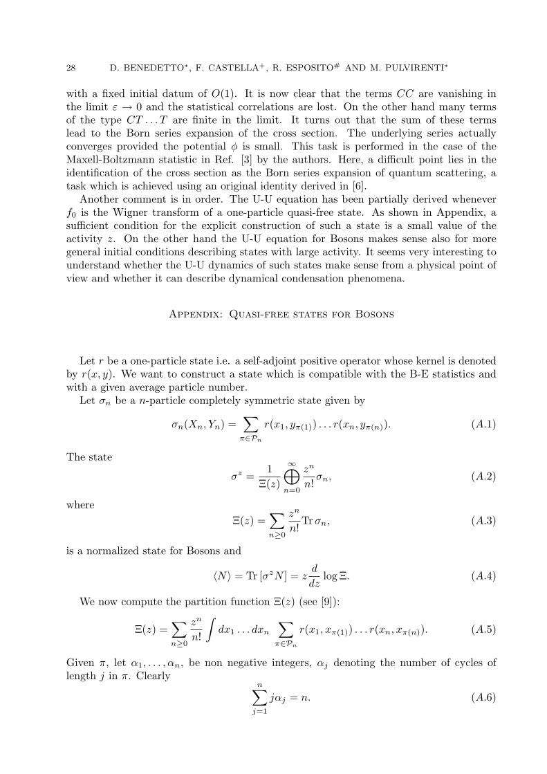
with a fixed initial datum of O(1). It is now clear that the terms CC are vanishing inthe limit ε → 0 and the statistical correlations are lost. On the other hand many termsof the type CT . . . T are finite in the limit. It turns out that the sum of these termslead to the Born series expansion of the cross section. The underlying series actuallyconverges provided the potential φ is small. This task is performed in the case of theMaxell-Boltzmann statistic in Ref. [3] by the authors. Here, a difficult point lies in theidentification of the cross section as the Born series expansion of quantum scattering, atask which is achieved using an original identity derived in [6].
Another comment is in order. The U-U equation has been partially derived wheneverf0 is the Wigner transform of a one-particle quasi-free state. As shown in Appendix, asufficient condition for the explicit construction of such a state is a small value of theactivity z. On the other hand the U-U equation for Bosons makes sense also for moregeneral initial conditions describing states with large activity. It seems very interesting tounderstand whether the U-U dynamics of such states make sense from a physical point ofview and whether it can describe dynamical condensation phenomena.
Appendix: Quasi-free states for Bosons
Let r be a one-particle state i.e. a self-adjoint positive operator whose kernel is denotedby r(x, y). We want to construct a state which is compatible with the B-E statistics andwith a given average particle number.
Let σn be a n-particle completely symmetric state given by
σn(Xn, Yn) =∑
π∈Pn
r(x1, yπ(1)) . . . r(xn, yπ(n)). (A.1)
The state
σz =1
Ξ(z)
∞⊕n=0
zn
n!σn, (A.2)
whereΞ(z) =
∑n≥0
zn
n!Trσn, (A.3)
is a normalized state for Bosons and
〈N〉 = Tr [σzN ] = zd
dzlog Ξ. (A.4)
We now compute the partition function Ξ(z) (see [9]):
Ξ(z) =∑n≥0
zn
n!
∫dx1 . . . dxn
∑π∈Pn
r(x1, xπ(1)) . . . r(xn, xπ(n)). (A.5)
Given π, let α1, . . . , αn, be non negative integers, αj denoting the number of cycles oflength j in π. Clearly
n∑j=1
jαj = n. (A.6)
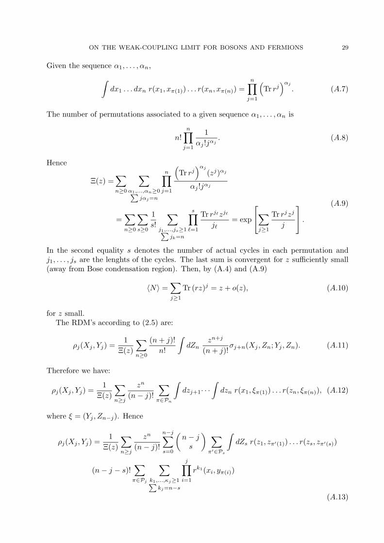
ON THE WEAK-COUPLING LIMIT FOR BOSONS AND FERMIONS 29
Given the sequence α1, . . . , αn,∫dx1 . . . dxn r(x1, xπ(1)) . . . r(xn, xπ(n)) =
n∏j=1
(Tr rj
)αj
. (A.7)
The number of permutations associated to a given sequence α1, . . . , αn is
n!n∏
j=1
1αj !jαj
. (A.8)
Hence
Ξ(z) =∑n≥0
∑α1,...,αn≥0∑
jαj=n
n∏j=1
(Tr rj
)αj
(zj)αj
αj !jαj
=∑n≥0
∑s≥0
1s!
∑j1,...,js≥1∑
jk=n
s∏`=1
Tr rj`zj`
j`= exp
∑j≥1
Tr rjzj
j
.
(A.9)
In the second equality s denotes the number of actual cycles in each permutation andj1, . . . , js are the lenghts of the cycles. The last sum is convergent for z sufficiently small(away from Bose condensation region). Then, by (A.4) and (A.9)
〈N〉 =∑j≥1
Tr (rz)j = z + o(z), (A.10)
for z small.The RDM’s according to (2.5) are:
ρj(Xj , Yj) =1
Ξ(z)
∑n≥0
(n + j)!n!
∫dZn
zn+j
(n + j)!σj+n(Xj , Zn;Yj , Zn). (A.11)
Therefore we have:
ρj(Xj , Yj) =1
Ξ(z)
∑n≥j
zn
(n− j)!
∑π∈Pn
∫dzj+1· · ·
∫dzn r(x1, ξπ(1)) . . . r(zn, ξπ(n)), (A.12)
where ξ = (Yj , Zn−j). Hence
ρj(Xj , Yj) =1
Ξ(z)
∑n≥j
zn
(n− j)!
n−j∑s=0
(n− j
s
) ∑π′∈Ps
∫dZs r(z1, zπ′(1)) . . . r(zs, zπ′(s))
(n− j − s)!∑
π∈Pj
∑k1,...,κj≥1∑
kj=n−s
j∏i=1
rk1(xi, yπ(i))
(A.13)

30 D. BENEDETTO∗, F. CASTELLA+, R. ESPOSITO# AND M. PULVIRENTI∗
with rk(x, y) the kernel of rk.Since (
n− js
)(n− j − s)!
(n− j)!=
1s!
, zn = zszn−s = zszΣk` , (A.14)
we obtain
ρj(Xj , Yj) =1
Ξ(z)
∑s≥0
zs
s!Trσs
∑π∈Pj
j∏`=1
∞∑k`=1
zk`rk`(x`, yπ(`)). (A.15)
Defining the one-particle operator
rz =∑k≥1
zkrk =zr
1− zr, (A.16)
for z sufficiently small, we arrive at
ρj(Xj , Yj) =∑
π∈Pj
rz(x1, yπ(1)) . . . rz(xj , yπ(j)), (A.17)
that is the characterization of the quasi-free state in terms of RDM.
ON THE WEAK-COUPLING LIMIT FOR BOSONS AND FERMIONS 31
References
[1] R.Balescu, Equilibrium and Nonequilibrium Statistical Mechanics, John Wiley & Sons, New York,
1975.[2] D. Benedetto, F. Castella, R. Esposito and M. Pulvirenti, Some Considerations on the derivation of
the nonlinear Quantum Boltzmann Equation, Jour. Statist. Phys. 116 1/4 (2004), 381–410.
[3] D. Benedetto, F. Castella, R. Esposito and M. Pulvirenti, In preparation.[4] O. Brattelli and D. W. Robinson, Operator Algebras and Quantum Statistical Mechanics, Texts and
Monographs in Physics, vol. 1, 2, Springer-Verlag.
[5] F. Castella, From the von Neumann equation to the Quantum Boltzmann equation in a deterministicframework, J. Statist. Phys. 104 1/2 (2001), 387–447.
[6] F. Castella, From the von Neumann equation to the Quantum Boltzmann equation II: identifying theBorn series, J. Statist. Phys. 106 5/6 (2002), 1197–1220.
[7] J. Dolbeault, Kinetic models and quantum effects: a modified Boltzmann equation for Fermi-Dirac
particles, Arch. Ration. Mech. Anal. 127 (1994), 101–131.[8] L. Erdos M Salmofer and H. T. Yau, On the Quantum Boltzmann Equation, Preprint.
[9] J.Ginibre, Some Applications of Functional Integration in Statistical Mechanics, Statistical Mechanics
and Field Theory (C. de Witt and R. Stora, eds.), Gordon and Breach, New York, 1970.[10] N. T. Ho and L. J.Landau, Fermi gas on a lattice in the van Hove limit, Jour. Statist. Phys. 87
(1997), 821–845.
[11] N. M. Hugenholtz, Derivation of the Boltzmann equation for a Fermi gas, Jour. Statist. Phys. 32(1983), 231–254.
[12] R. Jancel, Foundation of Classical and Quantum Statistical Mechanics, Pergamon Press, New York,
1969.[13] X. Lu, On spatially homogeneous solutions of a modified Boltzmann equation for Fermi-Dirac parti-
cles, Jour. Statist. Phys. 105 (2001), 353–388.[14] X. Lu, A modified Boltzmann equation for Bose-Einstein particles: isotropic solutions and long-time
behavior, Jour. Statist. Phys. 98 (2000), 1335–1394.
[15] X. Lu, B. Wennberg, On stability and strong convergence for spatially homogeneous Boltzmann equa-tion for Fermi-Dirac particles, Arch. Ration. Mech. Anal. 168 (2003), 1–34.
[16] H. Spohn, Quantum Kinetic Equations, On three levels: Micro-Meso and Macro Approaches in
Physics (M. Fannes, C. Maes, A. Verbeure, eds.), vol. 324, Nato ASI Series B: Physics, 1994, pp. 1–10.[17] E.A. Uehling and G.E. Uhlenbeck, Transport Phenomena in Einstein-Bose and Fermi-Dirac Gases.
I, Physical Review 43 (1933), 552–561.
[18] E. Wigner, On the Quantum Correction For Thermodynamic Equilibrium, Phys. Rev. 40 (1932),749–759.