On the Use of Time-Frequency Reassignmentin Additive Sound Modeling

Kelly Fitz and Lippold Haken

Abstract

We introduce the use of the method of reassignmentin sound modeling to produce a sharper, more robustadditive representation. TheReassigned Bandwidth-Enhanced Additive Modelfollows ridges in a time-frequency analysis to construct partials having both si-nusoidal and noise characteristics. This model yieldsgreater resolution in time and frequency than is possibleusing conventional additive techniques, and better pre-serves the temporal envelope of transient signals, even inmodified reconstruction, without introducing new com-ponent types or cumbersome phase interpolation algo-rithms.

0 Introduction

The method of reassignment has been used to sharpenspectrograms to make them more readable [1], to mea-sure sinusoidality, and to ensure optimal window align-ment in analysis of musical signals [2]. We usetime-frequency reassignment to improve ourBandwidth-Enhanced Additive Sound Model. The bandwidth-enhanced additive representation is similar in spirit totraditional sinusoidal models [3, 4, 5] in that a wave-form is modeled as a collection of components, calledpartials, having time-varying amplitude and frequencyenvelopes. Our partials are not strictly sinusoidal, how-ever. We employ a technique ofBandwidth Enhancementto combine sinusoidal energy and noise energy into asingle partial having time-varying amplitude, frequency,and bandwidth parameters [6, 7]. We use the methodof reassignment to improve the time and frequency es-timates used to define our partial parameter envelopes,thereby improving the time-frequency resolution of ourrepresentation, and improving its phase accuracy.

The combination of time-frequency reassignment andbandwidth enhancement yields a homogeneous model

(i.e. a model having a single component type) that iscapable of representing at high fidelity a wide variety ofsounds, including non-harmonic, polyphonic, impulsive,and noisy sounds. TheReassigned Bandwidth-EnhancedSound Modelis robust under transformation, and the fi-delity of the representation is preserved even under time-dilation and other model-domain modifications. The ho-mogeneity and robustness of the reassigned bandwidth-enhanced model make it particularly well-suited for suchmanipulations as cross synthesis and sound morphing.

Reassigned bandwidth-enhanced modeling and render-ing and many kinds of manipulations, including morph-ing, have been implemented in an open-source C++ classlibrary, Loris, and a stream-based, real time implementa-tion of bandwidth-enhanced synthesis is available in theSymbolic Sound Kyma environment.

1 Time-Frequency Reassignment

The discrete short-time Fourier transform is often usedas the basis for a time-frequency representation of time-varying signals, and is defined as a function of time indexn and frequency indexk as

Xn(k) =∞∑

l=−∞

h(l − n)x(l)e−j2π(l−n)k

N (1)

=

N−12∑

l=−N−12

h(l)x(n + l)e−j2πlk

N (2)

whereh(n) is a sliding window function equal to0 forn < −N−1

2 andn > N−12 (for N odd), so thatXn(k) is

theN -point discrete Fourier transform (DFT) of a short-time waveform centered at timen.

As a time-frequency representation, the STFT providesrelatively poor temporal data. Short-time Fourier datais sampled at a rate equal to the analysis hop size, sodata in derivative time-frequency representations is re-

1

ported on a regular temporal grid, corresponding to thecenters of the short-time analysis windows. The sam-pling of these so-calledframe-basedrepresentations canbe made as dense as desired by an appropriate choiceof hop size. Temporal smearing due to the long analy-sis windows needed to achieve high frequency resolutionpresents a much more serious problem that cannot be re-lieved by denser sampling.

Though the short-time phase spectrum is known to con-tain important temporal information, typically, only theshort-time magnitude spectrum is considered in the time-frequency representation. The short-time phase spectrumis sometimes used to improve the frequency estimatesin the time-frequency representation of quasi-harmonicsounds [8], but it is often omitted entirely, or used onlyin unmodified reconstruction, as in the Basic SinusoidalModel, described by McAulay and Quatieri [3].

It has been shown that partial derivatives of the short-time phase spectrum can be used to substantially improvethe short-time time and frequency resolution [9], and anefficient short-time Fourier transform-based implemen-tation has been developed that does not require complexdivision [1].

The so-calledMethod of Reassignmentcomputes re-assigned time and frequency estimates for each spec-tral component from partial derivatives of the short-timephase spectrum. Instead of locating time-frequency com-ponents at the geometrical center of the analysis win-dow (tn, ωk), as in traditional short-time spectral analy-sis, the components are reassigned to the center of grav-ity of their complex spectral energy distribution, com-puted from the short-time phase spectrum according tothe principle of stationary phase. This method was firstdeveloped in the context of the spectrogram and calledtheModified Moving Window Method[9], but has sincebeen applied to a variety of time-frequency and time-scale transforms [1].

The theorem of stationary phase states that the variationof the Fourier phase spectrum not attributable to periodicoscillation is slow with respect to frequency in certainspectral regions, and in surrounding regions the varia-tion is relatively rapid. In Fourier reconstruction, pos-itive and negative contributions to the waveform cancelin frequency regions of rapid phase variation. Only re-gions of slow phase variation (stationary phase) will con-tribute significantly to the reconstruction, and the maxi-mum contribution (center of gravity) occurs at the pointwhere the phase is changing most slowly with respect totime and frequency.

In the vicinity of t = τ (i.e., for an analysis windowcentered at timet = τ ), the point of maximum spectralenergy contribution has time-frequency coordinates thatsatisfy the stationarity conditions

∂

∂ω[φ (τ, ω) + ω · (t − τ)] = 0 (3)

∂

∂τ[φ (τ, ω) + ω · (t − τ)] = 0 (4)

whereφ (τ, ω) is the continuous short-time phase spec-trum andω · (t − τ) is the phase travel due to periodicoscillation [9]. The stationarity conditions are satisfiedat the coordinates

t = τ − ∂φ (τ, ω)∂ω

(5)

ω =∂φ (τ, ω)

∂τ(6)

representing, respectively, the group delay and instanta-neous frequency.

Discretizing Equations (5) and (6) to compute the timeand frequency coordinates numerically is difficult andunreliable, because the partial derivatives must be ap-proximated. These formulae can be rewritten in the formof ratios of discrete Fourier transforms [1]. Time andfrequency coordinates can be computed using two ad-ditional short-time Fourier transforms, one employinga time-weighted window function and one employing afrequency-weighted window function.

Since time estimates correspond to the temporal center ofthe short-time analysis window, the time-weighted win-dow is computed by scaling the analysis window func-tion by a time ramp the time ramp from−N−1

2 to N−12 ,

for a window of lengthN . The frequency-weighted win-dow is computed by wrapping the Fourier transform ofthe analysis window to the frequency range[−π, π], scal-ing the transform by a frequency ramp from−N−1

2 toN−1

2 , and inverting the scaled tranform to obtain a (real)frequency-scaled window. Using these weighted win-dows, the method of reassignment computes correctionsto the time and frequency estimates in fractional sampleunits between−N−1

2 and N−12 . The three analysis win-

dows employed in reassigned short-time Fourier analysisare shown in Figure 1.

The method of reassignment computes reassigned timesa frequencies for each short-time spectral component.The reassigned time,tk,n, for the kth spectral compo-nent from the short-time analysis window centered attime n (in samples, assuming odd-length analysis win-

2

−250 −200 −150 −100 −50 0 50 100 150 200 250

0.2

0.4

0.6

0.8

1

Analysis windows used in time−frequency reassignment

n

h(n)

−250 −200 −150 −100 −50 0 50 100 150 200 250

−40

−20

0

20

40

n

h t(n)

−250 −200 −150 −100 −50 0 50 100 150 200 250

−100

0

100

n

h f(n)

Figure 1: Analysis windows employed in the three short-time transforms used to compute reassigned times andfrequencies. Waveform (a) is the original window func-tion, h (n) (a 501 point Kaiser window with shapingparameter 12.0, in this case), waveform (b) is time-weighted window function,ht (n) = n h (n), and wave-form (c) is the frequency-weighted window function,hf (n).

dows) is [1]

tk,n = n −<

{Xt;n(k)X∗

n(k)|Xn(k)|2

}(7)

whereXt;n(k) denotes the short-time transform com-puted using the time-weighted window function and<{·} denotes the real part of the bracketed ratio.

The corrected frequency,ωk,n corresponding to the samecomponent is [1]

ωk,n = k + =

{Xf ;n(k)X∗

n(k)|Xn(k)|2

}(8)

whereXf ;n(k) denotes the short-time transform com-puted using the frequency-weighted window functionand={·} denotes the imaginary part of the bracketed ra-tio. Both tk,n andωk,n have units of fractional samples.

Time and frequency shifts are preserved in the reassign-ment operation, and energy is conserved in the reas-signed time-frequency data. Moreover, chirps and im-pulses are perfectly localized in time and frequency inany reassigned time-frequency or time-scale representa-tion [1]. Reassignment sacrifices the bilinearity of time-frequency transformations like the squared magnitude ofthe short-time Fourier transform, since every data point

in the representation is relocated by a process that ishighly signal dependent. This is not an issue in our repre-sentation, since the bandwidth-enhanced additive model,like the basic sinusoidal model [3], retains data only attime-frequency ridges (peaks in the short-time magni-tude spectra), and thus is not bilinear.

Note that, since the short-time Fourier transform is in-vertible, and the original waveform can be exactly recon-structed from an adequately-sampled short-time Fourierrepresentation, all the information needed to precisely lo-cate a spectral component within an analysis window ispresent in the short-time coefficients,Xn(k). Temporalinformation is encoded in the short-time phase spectrum,which is very difficult to interpret. The method of reas-signment is a technique for extracting information fromthe phase spectrum.

2 Reassigned Bandwidth-Enhanced Analysis

The method of reassignment has been used to sharpenspectrograms to make them more readable [1, 10].We use it to improve our bandwidth-enhanced sinu-soidal modeling representation [6, 7]. TheReas-signed Bandwidth-Enhanced Additive Model[11] em-ploys time-frequency reassignment to improve the timeand frequency estimates used to define our partial param-eter envelopes, thereby improving the time-frequencyresolution of our representation, and improving its phaseaccuracy.

Reassignment transforms our analysis from a frame-based analysis into a “true” time-frequency analysis.Whereas the discrete short-time Fourier transform de-fined by Equation 2 orients data according to the anal-ysis frame rate and the length of the transform, the timeand frequency orientation of reassigned spectral data issolely a function of the data itself.

The method of analysis we use in our research models asampled audio waveform as a collection ofbandwidth-enhanced partialshaving sinusoidal and noise-like char-acteristics. Bandwidth-enhanced partials are defined bya trio of synchronized breakpoint envelopes specifyingthe time-varying amplitude, center frequency, and noisecontent for each component. Each partial is rendered byabandwidth-enhanced oscillator, described by

y(n) = [A(n) + β(n)ζ(n)] cos (θ(n)) (9)

3

+

y(n)

β(n) A(n)

ζ(n)

noise lowpass filter

ω(n)

N

Figure 2: Block diagram of the Bandwidth-EnhancedOscillator. The time-varying sinusoidal and noise ampli-tudes are controlled byA(n) andβ(n), respectively, andthe time-varying center (sinusoidal) frequency isω(n).

whereA(n) and β(n) are the time-varying sinusoidaland noise amplitudes, respectively, andζ(n) is a energy-normalized lowpass noise sequence, generated by excit-ing a lowpass filter with white noise and scaling the filtergain such that the noise sequence has the same total spec-tral energy as a full-amplitude sinusoid. The oscillatorphaseθ(n), is initialized to some starting value, obtainedfrom the reassigned short-time phase spectrum, and up-dated according to the time-varying radian frequency,ω(n), by

θ(n) = θ(n − 1) + ω(n) n > 0 (10)

The bandwidth-enhanced oscillator is depicted in Fig-ure 2.

We define the time-varyingbandwidth coefficient, κ(n),as the fraction of total instantaneous partial energy that isattributable to noise. This bandwidth (or noisiness) co-efficient assumes values between0 for a pure sinusoidand1 for partial that is entirely narrowband noise, andvaries over time according to the noisiness of the partial.If we represent the total (sinusoidal and noise) instan-taneous partial energy asA2(n), then the output of thebandwidth-enhanced oscillator is described by

y(n) = A(n)[√

1 − κ(n) +√

2κ(n)ζ(n)]cos (θ(n))

(11)

The envelopes for the time-varying partial amplitudesand frequencies are constructed by identifying and fol-lowing ridges on the time-frequency surface. The time-varying partial bandwidth coefficients are computed andassigned by a process ofbandwidth association[6].

We use the method of reassignment to improve the time

and frequency estimates for our partial parameter en-velope breakpoints by computing reassigned times andfrequencies that are not constratined to lie on the time-frequency grid defined by the short-time Fourier anal-ysis parameters. Our algorithm shares with traditionalsinusoidal methods the notion of temporally connectedpartial parameter estimates, but by contrast, our esti-mates are non-uniformly distributed in both time and fre-quency, as shown in Figure 3.

Short-time analysis windows normally overlap in bothtime and frequency, so time-frequency reassignment of-ten yields time corrections greater than the length of theshort-time hop size and frequency corrections greaterthan the width of a frequency bin. Large time correctionsare common in analysis windows containing strong tran-sients that are far from the temporal center of the win-dow. Since we retain data only at time-frequency ridges,that is, at frequencies of spectral energy concentration,we generally observe large frequency corrections only inthe presence of strong noise components, where phasestationarity is a weaker effect. The analysis data depictedin Figure 3c shows many data points reassigned to timesnear an apparent transient, resulting in a cluster of datanear the time of the transient, but eliminating the tempo-ral smearing characteristic of frame-based analysis tech-niques.

3 Sharpening Transients

Time-frequency representations based on traditionalmagnitude-only short-time Fourier analysis techniques(such as the spectrogram and the basic sinusoidalmodel [3]) fail to distinguish transient components fromsustaining components. A strong transient waveform, asshown in Figure 4a, is represented by a collection oflow amplitude spectral components in early short-timeanalysis frames, that is, frames corresponding to analy-sis windows centered earlier than the time of the tran-sient. A low-amplitude periodic waveform, as shown inFigure 4b, is also represented by a collection of low am-plitude spectral components. The information needed todistinguish these two critically different waveforms is en-coded in the short-time phase spectrum, and is extractedby the method of reassignment.

Other methods have been proposed for representing tran-sient waveforms in additive sound models. Verma andMeng [12] introduce new component types specificallyfor modeling transients, but this method sacrifices the ho-

4

ω8

ω7

ω6

ω5

ω4

ω3

ω2

ω1

t1 t2 t3 t4 t5 t6 t7

ω8

ω7

ω6

ω5

ω4

ω3

ω2

ω1

t1 t2 t3 t4 t5 t6 t7

ω8

ω7

ω6

ω5

ω4

ω3

ω2

ω1

t1 t2 t3 t4 t5 t6 t7

Time

Freq

uenc

y

TimeFr

eque

ncy

Time

Freq

uenc

y

(a) (b) (c)

Figure 3: Comparison of time-frequency data included in common representations. Only the time-frequency orien-tation of the data points is shown. The short-time Fourier transform (a) retains data at every timetn and frequencyωk. The basic sinusoidal model [3] retains data at selected time and frequency samples, as shown in (b). Reassignedbandwidth-enhanced analysis data (c) is distributed continuously in time and frequency, and retained only at time-frequency ridges. Arrows indicate the mapping of short-time spectral samples onto time-frequency ridges due to themethod of reassignment.

0 100 200 300 400 500 600 700−0.2

0

0.2

0.4

0.6

0.8

1

time

0 100 200 300 400 500 600 700−0.2

0

0.2

0.4

0.6

0.8

1

time

Figure 4: Two windowed short-time waveforms (dashedlines) that are not readily distinguished in the basic sin-soidal model [3]. Both waveforms are represented bylow-amplitude spectral components, and with reassign-ment, the strong transient on the left (a) yields off-centercomponents, having large time corrections (positive inthis case because the transient is near the right tail of thewindow), while the sustained quasi-periodic waveformon the right (b) yields time corrections near zero.

mogeneity of the model. A homogeneous model, thatis, a model having a single component type, such asthe breakpoint parameter envelopes in our reassignedbandwidth-enhanced additive model [11], is critical formany kinds of manipulations [13, 14]. Peeters andRodet [2] have developed a hybrid analysis/synthesissystem that eschews high-level transient models and re-tains unabridgedOLA (overlap-add) frame data at tran-sient positions. This hybrid representation representsunmodified transients perfectly, but also sacrifices ho-mogenity. Quatieri [15] proposes a method for preserv-ing the temporal envelope short-duration complex acous-tic signals using a homogeneous sinsusoidal model, butit is inapplicable to longer duration sounds, or soundshaving multiple transient events.

Time-frequency reassignment allows us to preserve tem-poral envelope shape without sacrificing the homogene-ity of the bandwidth-enhanced additive model. Reas-signment greatly improves time resolution by relocatingspectral peaks closer to the time of the transient events,so that transients are not smeared out by the length ofthe analysis window. Components extracted from earlyor late short-time analysis windows are reassigned totimes near the time of the transient, yielding clusters oftime-frequency data points, as shown in the reassignedanalysis depicted in Figure 3. Moreover, since reas-signment sharpens our frequency estimates, it is possi-ble to achieve good frequency resolution with shorter (intime) analysis windows than would be possible with tra-ditional methods. The use of shorter analysis windows

5

60 310−1

0

1

Time

Am

plitu

de

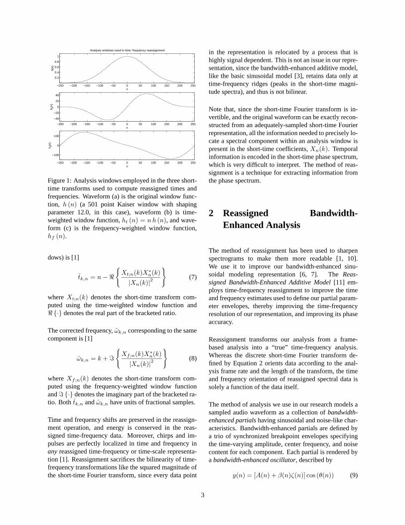
Figure 5: Two long analysis windows superimposed atdifferent times on a square wave signal with an abruptturn-on. The short-time transform corresponding to theearlier window generates unreliable parameter estimatesand smears the sharp onset of the square wave.

further improves our time resolution and reduces tempo-ral smearing.

The effect of time-frequency reassignment on transientresponse can be demonstrated using a square wave thatturns on abruptly, shown in Figure 5. This waveform,while aurally uninteresting and uninformative, is use-ful for visualizing the performance of various analysismethods. Its abrupt onset makes temporal smearing ob-vious, its simple harmonic partial amplitude relationshipmakes it easy to predict the necessary data for a goodtime-frequency representation, and its simple waveshapemakes phase errors and temporal distortion easy to iden-tify. Note, however, that this waveform is pathologicalfor Fourier-based additive models, and exaggerates all ofthese problems with such methods. We use it only forcomparison of various methods.

Figures 6 and 7 show two reconstructions of the onsetof the square wave in Figure 5 from time-frequency dataobtained using a 54-ms analysis window. The silencebefore the onset is not shown. Only the first (lowestfrequency) five harmonic partials were used in the re-construction, and consequently the ringing due to Gibb’sphenomenon is evident.

Figure 6 is a reconstruction from traditional, nonreas-signed time-frequency data. The reconstructed squarewave amplitude rises very gradually and reaches full am-plitude approximately 40 ms after the first non-zero sam-ple. Clearly, the instantaneous turn-on has been smeared

out by the long analysis window. Figure 7 shows a recon-struction from reassigned time-frequency data. The tran-sient response has been greatly improved by relocatingcomponents extracted from early analysis windows (likethe one on the left in Figure 5) to their spectral centersof gravity, closer to the observed turn-on time. The syn-thesized onset time has been reduced to approximately10 ms. The time-frequency analysis data is shown inFigure 8. The nonreassigned data is evenly distributed intime, so data from early windows (that is, windows cen-tered before the onset time) smears the onset, whereas thereassigned data from early analysis windows is clumpednear the correct onset time.

4 Cropping

Off-centercomponents are short-time spectral compo-nents having large time reassignments, that is, compo-nents having centers of gravity far from the temporal cen-ter of the analysis window. Since they represent transientevents that are far from the center of the analysis window,and are therefore poorly represented in the windowedshort-time waveform, these off-center components intro-duce unreliable spectral parameter estimates that corruptour representation, making the model data difficult to in-terpret and manipulate.

Fortunately, large time corrections make off-center com-ponents easy to identify and remove from our model.By removing the unreliable data embodied by off-centercomponents, we make our model cleaner and more ro-bust. Moreover, thanks to the redundancy inherent inshort-time analysis with overlapping analysis windows,we do not sacrifice information by removing the unre-liable data points. The information represented poorlyin off-center components is more reliably represented inwell-centered components, extracted from analysis win-dows centered nearer the time of the transient event. Fig-ure 9 shows reassigned bandwidth-enhanced model datafrom the onset of a bowed cello tone before and after theremoval of off-center components. Typically, data hav-ing time corrections greater than the time between con-secutive analysis window centers is considered to be un-reliable, and is removed, orcropped.

Cropping partials to remove off-center components al-lows us to localize transient events reliably. Figure 8(c)shows reassigned time-frequency data from the abruptsquare wave onset with off-center components removed.The abrupt square wave onset synthesized from the

6

4422

0 22Time (ms)

Am

plitu

de

Time (ms)

Am

plitu

de

Figure 6: Onset of square wave reconstruction without reassignment.

0 22Time (ms)

Am

plitu

de

Figure 7: Onset of square wave reconstruction with reassignment.

2000

00 60Time (ms)

Freq

uenc

y (H

z)

(a)

2000

00 60Time (ms)

Freq

uenc

y (H

z)

(b )

2000

00 60Time (ms)

Freq

uenc

y (H

z)

(c)

Figure 8: Time-frequency analysis data points for an abrupt square wave onset, depicted in Figure 5. The traditionalnonreassigned data (a) is evenly distributed in time, whereas the reassigned data (b) is clumped at the onset time. (c)shows the reassigned analysis data after far off-center components have been removed, or “cropped”. Only time andfrequency information is plotted, amplitude information is not displayed.

7

(a)

(b)

Time (ms)

Freq

uenc

y (H

z)

0 140370

1200

Time (ms)

Freq

uenc

y (H

z)

0 140370

1200

Figure 9: Time-frequency coordinates of data from reas-signed bandwidth-enhanced analysis before (a) and after(b) cropping of off-center components clumped togetherat partial onsets. The source waveform is a bowed cellotone.

cropped reassigned data, seen in Figure 10, is muchsharper than the uncropped, reassigned reconstruction,because the taper of the analysis window makes eventhe time correction data unreliable in components thatare very far off-center. Figure 9 shows reassignedbandwidth-enhanced model data from the onset of abowed cello tone before and after the removal of off-center components. In this case, components with timecorrections greater than 10 milliseconds (the time be-tween consecutive analysis windows) were deemed to betoo far off-center to deliver reliable parameter estimates.As in Figure 8(c), the unreliable data clustered at the timeof the onset is removed, leaving a cleaner, more robustrepresentation.

5 Phase Maintenance

Preserving phase is important for reproducing someclasses of sounds, particularly transients and short-duration complex audio events having significant infor-mation in the temporal envelope [15]. The basic sinu-soidal model proposed by McAulay and Quatieri [3] isphase correct, that is, it preserves phase at all times in

unmodified reconstruction. In order to match short-timespectral frequency and phase estimates at frame bound-aries, McAulay and Quatieri employ cubic interpolationof the instantaneous partial phase.

Cubic phase envelopes have many undesirable proper-ties. They are difficult to manipulate and maintain un-der time- and frequency-scale transformation comparedto linear frequency envelopes. However, in unmodifiedreconstruction, cubic interpolation prevents the propa-gation of phase errors introduced by unreliable param-eter estimates, maintaining phase accuracy in transients,where the temporal envelope is important, and through-out the reconstructed waveform. The effect of phase er-rors in unmodified reconstruction of a square wave isillustrated in Figure 11. If not corrected using a tech-nique like cubic phase interpolation, partial parametererrors introduced by off-center components render thewave shape visually unrecognizable. Figure 12 showsthat cubic phase can be used to correct these errors inunmodified reconstruction. It should be noted that inthis case, the phase errors appear dramatic, but are notimportant to the sound of the reconstructed waveform.In many sounds, particularly transient sounds, preserva-tion of the temporal envelope is critical [15, 12], but thesquare waveforms in Figures 11 and 12 sound identical.It should also be noted that cubic phase interpolation canbe used to preserve phase accuracy, but does not reducetemporal smearing due to off-center components in longanalysis windows.

It is not desirable to preserve phase at all times inmodified reconstruction. Because frequency is the timederivative of phase, any change in the time or frequencyscale of a partial must correspond to a change in thephase values at the parameter envelope breakpoints.

In general, preserving phase using the cubic phasemethod in the presence of modifications (or estimationerrors) introduces wild frequency excursions [16]. Phasecan be preserved at one time, however, and that time istypically chosen to be the onset of each partial, althoughany single time could be chosen. The partial phase at allother times is modified to reflect the new time-frequencycharacteristic of the modified partial.

Off-center components with unreliable parameter esti-mates introduce phase errors in modified reconstruction.If the phase is maintained at the partial onset, even thecubic interpolation scheme cannot prevent phase errorsfrom propagating in modified syntheses. This effect isillustrated in Figure 13, in which the square wave time-frequency data has been shifted in frequency by 10% and

8

0 22Time (ms)

Am

plitu

de

Figure 10: Onset of square wave reconstruction with reassignment and removal of unreliable partial parameter esti-mates.

reconstructed using cubic phase curves modified to re-flect the frequency shift.

By removing the off-center components at the onset of apartial, we not only remove the primary source of phaseerrors, we also improve the shape of the temporal enve-lope in modified reconstruction of transients by preserv-ing a more reliable phase estimate at a time closer to thetime of transient event. We can therefore maintain phaseaccuracy at critical parts of the audio waveform evenunder transformation, and even using linear frequencyenvelopes, which are much simpler to compute, inter-pret, edit, and maintain than cubic phase curves. Fig-ure 14 shows a square wave reconstruction from croppedreassigned time-frequency data, and Figure 15 shows afrequency-shifted reconstruction, both using linear fre-quency interpolation. Removing components with largetime corrections preserves phase in modified and unmod-ified reconstruction, and thus obviates cubic phase inter-polation.

Moreover, since we do not rely on frequent cubic phasecorrections to our frequency estimates to preserve theshape of the temporal envelope (which would otherwisebe corrupted by errors introduced by unreliable data),we have found that we can obtain very good-quality re-construction, even under modification, with regularly-sampled partial parameter envelopes. That is, we cansample the frequency, amplitude, and bandwidth en-velopes of our reassigned bandwidth-enhanced partials atregular intervals (of, for example, 8 milliseconds) with-out sacrificing the fidelity of the model. We therebyachieve the data regularity of frame-based additive modeldata and the fidelity of reassigned spectral data. Resam-pling of the partial parameter envelopes is especially use-ful in real-time synthesis applications [13, 14].

6 Breaking partials at TransientEvents

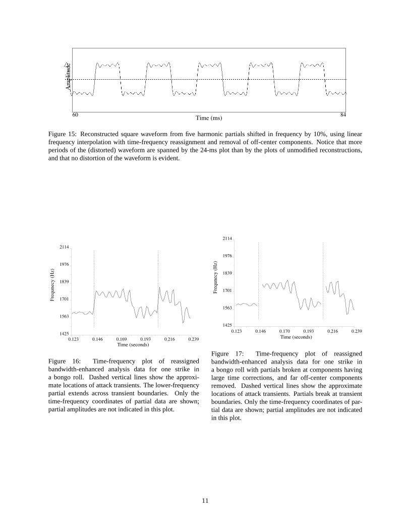
Transients corresponding to the onset of all associatedpartials are preserved in our model by removing off-center components at the ends of partials. If transients al-ways correspond to the onset of associated partials, thenthat method will preserve the temporal envelope of multi-ple transient events. In fact, however, partials often spantransients. Figure 16 shows a partial that extends overtransient boundaries in a representation of a bongo roll,a sequence of very short transient events. The approxi-mate attack times are indicated by dashed vertical lines.In such cases, it is not possible to preserve the phase atthe locations of multiple transients, since, under modifi-cation the phase can only be preserved at one time in thelife of a partial.

Strong transients are identified by the large time correc-tions they introduce. By breaking partials at componentshaving large time corrections, we cause all associatedpartials to be born at the time of the transient, and therebyenhance our ability to maintain phase accuracy. In Fig-ure 17, the partial that spanned several transients in Fig-ure 16 has been broken at components having time cor-rections greater than the time between successive analy-sis window centers (about 1.3 milliseconds, in this case),allowing us to maintain the partial phases at each bongostrike. By breaking partials at the locations of transients,we can preserve the temporal envelope of multiple tran-sient events, even under transformation.

Figure 18 shows the waveform for two strikes in a bongoroll reconstructed from reassigned bandwidth-enhanceddata. The same two bongo strikes reconstructed fromnonreassigned data are shown in Figure 19. Comparisonto the source waveform shown in Figure 20 reveals that

9

60 84Time (ms)

Am

plitu

de

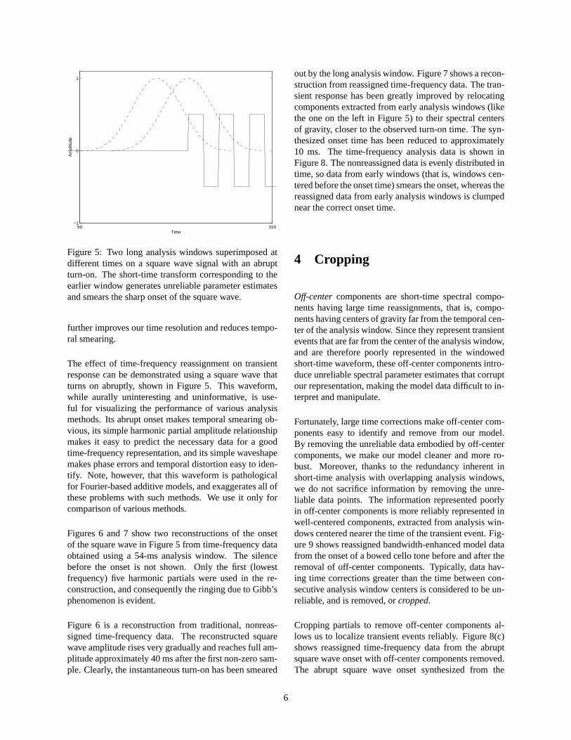
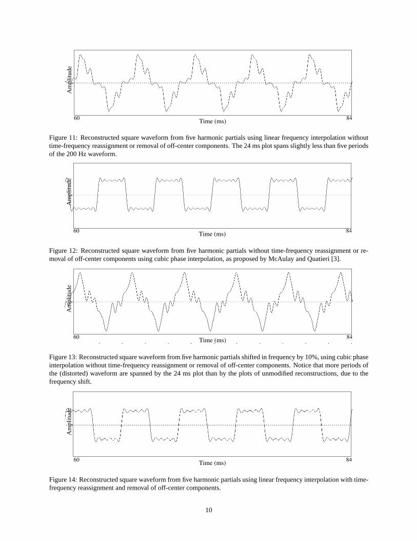
Figure 11: Reconstructed square waveform from five harmonic partials using linear frequency interpolation withouttime-frequency reassignment or removal of off-center components. The 24 ms plot spans slightly less than five periodsof the 200 Hz waveform.

60 84Time (ms)

Am

plitu

de

Figure 12: Reconstructed square waveform from five harmonic partials without time-frequency reassignment or re-moval of off-center components using cubic phase interpolation, as proposed by McAulay and Quatieri [3].

60 84Time (ms)

Am

plitu

de

Figure 13: Reconstructed square waveform from five harmonic partials shifted in frequency by 10%, using cubic phaseinterpolation without time-frequency reassignment or removal of off-center components. Notice that more periods ofthe (distorted) waveform are spanned by the 24 ms plot than by the plots of unmodified reconstructions, due to thefrequency shift.

60 84Time (ms)

Am

plitu

de

Figure 14: Reconstructed square waveform from five harmonic partials using linear frequency interpolation with time-frequency reassignment and removal of off-center components.

10

60 84Time (ms)

Am

plitu

de

Figure 15: Reconstructed square waveform from five harmonic partials shifted in frequency by 10%, using linearfrequency interpolation with time-frequency reassignment and removal of off-center components. Notice that moreperiods of the (distorted) waveform are spanned by the 24-ms plot than by the plots of unmodified reconstructions,and that no distortion of the waveform is evident.

0.2390.2160.1930.1690.1460.123

2114

1976

1839

1701

1563

1425

Time (seconds)

Freq

unec

y (H

z)

Figure 16: Time-frequency plot of reassignedbandwidth-enhanced analysis data for one strike ina bongo roll. Dashed vertical lines show the approxi-mate locations of attack transients. The lower-frequencypartial extends across transient boundaries. Only thetime-frequency coordinates of partial data are shown;partial amplitudes are not indicated in this plot.

0.2390.2160.1930.1700.1460.123

2114

1976

1839

1701

1563

1425

Time (seconds)

Freq

unec

y (H

z)

Figure 17: Time-frequency plot of reassignedbandwidth-enhanced analysis data for one strike ina bongo roll with partials broken at components havinglarge time corrections, and far off-center componentsremoved. Dashed vertical lines show the approximatelocations of attack transients. Partials break at transientboundaries. Only the time-frequency coordinates of par-tial data are shown; partial amplitudes are not indicatedin this plot.

11

the reconstruction from reassigned data is better able topreserve the temporal envelope than the reconstructionfrom nonreassigned data and suffers less from temporalsmearing.

7 Real–Time Synthesis

Together with Kurt Hebel of Symbolic Sound Corpo-ration, we have implemented a real-time reassignedbandwidth-enhanced synthesizer using the Kyma SoundDesign Workstation [17].

Many real-time synthesis systems allow the sound de-signer to manipulate streams of samples. In our real-time reassigned bandwidth-enhanced implementation,we work with streams of data that are not time-domainsamples. Rather, ourEnvelope Parameter Streamsen-code frequency, amplitude, and bandwidth envelope pa-rameters for each bandwidth-enhanced partial [13, 14].

Much of the strength of systems that operate on sam-ple streams is derived from the uniformity of the data.This homogeneity gives the sound designer great flexi-bility with a few general-purpose processing elements.In our encoding of envelope parameter streams, data ho-mogeneity is also of prime importance. The envelopeparameters for all the partials in a sound are encoded se-quentially. Typically, the stream has ablock sizeof 128samples, which means the parameters for each partial areupdated every 128 samples, or 2.9 ms at a 44.1 kHz sam-pling rate. Sample streams generally do not have blocksizes associated with them, but this structure is neces-sary in our envelope parameter stream implementation.The envelope parameter stream encodes envelope infor-mation for a single partial at each sample time, and ablock of samples provides updated envelope informationfor all the partials.

Envelope parameter streams are usually created bytraversing a file containing frame-based data from ananalysis of a source recording. Such a file can be de-rived from a reassigned bandwidth-enhanced analysis byresampling the envelopes at 2.9 ms intervals. The param-eter streams may also be generated by real-time analysis,or by real-time algorithms, but that process is beyond thescope of this discussion. A parameter stream typicallypasses through several processing elements. These pro-cessing elements can combine multiple streams in a va-riety of ways, and can modify values within a stream.Finally, a synthesis element computes an audio sample

stream from the envelope parameter stream.

Our real-time synthesis element implements bandwidth-enhanced oscillators [7] with the sum

y(n) =K−1∑k=0

[Ak(n) + Nk(n)b(n)] sin θk(n)(12)

θk(n) = θk(n − 1) + 2Fk(n) (13)

where

• y is the time domain waveform for the synthesizedsound,

• n is the sample number,

• k is the partial number in the sound,

• K is the total number of partials in the sound (usu-ally between 20 and 160),

• Ak is partialk’s amplitude envelope,

• Nk is partialk’s noise envelope,

• b is a zero-mean noise modulator with bell-shapedspectrum,

• Fk is partialk’s log (base 2) frequency envelope,

• θk is the running phase for thekth partial.

Values for the envelopesAk, Nk, andFk are updatedfrom the parameter stream every 2.9 ms. The synthesiselement performs sample-level linear interpolation be-tween updates, so thatAk, Nk, andFk are piecewise lin-ear envelopes with 2.9 ms linear segments [18]. Theθk

values are initialized at partial onsets (whenAk andNk

are zero) from the phase envelope in the partial’s param-eter stream.

Rather than use a separate model to represent noise in oursounds, we use the envelopeNk (in addition to the tra-ditional Ak andFk envelopes) and retain a homogenousdata stream. Quasi-harmonic sounds, even those withnoisy attacks, have one partial per harmonic in our rep-resentation. The noise envelopes allow a sound designerto manipulate noise-like components of sound in an in-tuitive way, using a familiar set of controls. We have im-plemented a wide variety of real-time manipulations onenvelope parameter streams, including frequency shift-ing, formant shifting, time dilation, cross synthesis, andsound morphing.

12

Time (s)

Am

plitu

de

0.14 0.25

Figure 18: Waveform plot for two strikes in a bongo roll reconstructed from reassigned bandwidth-enhanced data.

Time (s)

Am

plitu

de

0.14 0.25

Figure 19: Waveform plot for two strikes in a bongo roll reconstructed from nonreassigned bandwidth-enhanced data,synthesized using cubic phase interpolation to maintain phase accuracy.

Time (s)

Am

plitu

de

0.14 0.25

Figure 20: Plot of the source waveform for the bongo strikes analyzed and reconstructed in Figures 18 and 19.

13

Our new MIDI controller, the Continuum Fingerboard,allows continuous control over each note in a perfor-mance. It resembles a traditional keyboard in that it isapproximately the same size and is played with ten fin-gers [14]. Like keyboards supporting MIDI’s polyphonicaftertouch, it continually measures each finger’s pres-sure. The Continuum Fingerboard also resembles a fret-less string instrument in that it has no discrete pitches;any pitch may be played, and smooth glissandi are possi-ble. It tracks thex, y, z position for each finger pressingon the playing surface. These continuous 3-dimensionaloutputs are a convenient source of control parameters forreal-time manipulations on envelope parameter streams.

8 Conclusions

The reassigned bandwidth-enhanced additive soundmodel [11] combines bandwidth-enhanced analysis andsynthesis techiniques [6, 7] with the time-frequency re-assignment technique described in this paper.

We have found that the method of reassignment dra-matically strengthens our bandwidth-enhanced additivesound model. Temporal smearing is greatly reduced be-cause the time-frequency orientation of the model datais waveform-dependent, rather than analysis-dependentas in traditional short-time analysis methods. Moreover,time-frequency reassignment allows us to identify unreli-able data points (having bad parameter estimates) and re-move them from the representation. This not only sharp-ens the representation and makes it more robust, but italso allows us to maintain phase accuracy at transients,even under transformation, while avoiding the problemsassociated with cubic phase interpolation.

A Results

The reassigned bandwidth-enhanced additive model isimplemented in the open source C++ class libraryLoris [19], and is the basis of the sound manipulationand morphing algorithms implemented therein.

We have attempted to use a wide variety of sounds inthe experiments we conducted during the developmentof the reassigned bandwidth-enhanced additive soundmodel. The results from a few of those experiments arepresented in this section. Data and waveform plots are

not intended to constitute proof of the efficacy of ouralgorithms, or the utility of our representation. Theyare intended only to illustrate features of some of thesounds used and generated in our experiments. The re-sults of our work can only be judged by auditory eval-uation, and to that end, these sounds and many oth-ers are available for audition at the Loris web site,www.cerlsoundgroup.org/Loris .

All sounds used in these experiments were sampled at44.1 kHz (CD quality), so time-frequency analysis datais available at frequencies as high as 22.05 kHz. How-ever, for clarity, only a limited frequency range is plot-ted in most cases. Spectrogram plots all have high gainso that low-amplitude high-frequency partials are visible.Consequently, strong low-frequency partials are very of-ten clipped, and appear to have unnaturally flat amplitudeenvelopes.

Waveform and spectrogram plots were produced usingAlberto Ricci’s SoundMakersoftware application [20].Plots of sinusoidal and bandwidth-enhanced analysisdata were produced using unreleased development ver-sions of theLoris software application [19]. In plotsof bandwidth-enhanced analysis data, partial center fre-quencies are plotted against time, and partial amplitude isindicated by grayscale, with darker lines correspondingto higher amplitude. Partial bandwidth is not indicatedon these plots.

A.1 Flute Tone

A flute tone, played at pitch D4 (D above middle C), hav-ing a fundamental frequency of approximately 293 Hzand no vibrato, taken from the McGill University Mas-ter Samples compact discs [21, Disc 2 Track 1 Index 3]is shown in the 3D spectrogram plot in Figure 21. Thissound was modeled by reassigned bandwidth-enhancedanalysis data produced using a 53 ms Kaiser analysiswindow with 90 dB sidelobe rejection. The partialswere constrained to be separated by at least 250 Hz,slightly greater than 85% of the harmonic partial sepa-ration. Breath noise is a significant component of thissound. This noise is visible between the strong harmoniccomponents in the spectrogram plot, particularly at fre-quencies above 3 kHz. The breath noise is faithfullyrepresented in the reassigned bandwidth-enhanced anal-ysis data, and reproduced in the reconstructions from thatanalysis data. A 3D spectrogram plot of the reconstruc-tion is shown in Figure 22. The absence of the breathnoise is apparent in spectral plot for sinusoidal recon-

14

struction from non-bandwidth-enhanced analysis data,shown in Figure 23.

A.2 Cello Tone

A cello tone, played at pitch D sharp 3 (D sharp be-low middle C), having a fundamental frequency of ap-proximately 156 Hz, played by Edwin Tellman andrecorded by Patrick Wolfe [22] was modeled by reas-signed bandwidth-enhanced analysis data produced us-ing a 71 ms Kaiser analysis window with 80 dB side-lobe rejection. The partials were constrained to be sep-arated by at least 135 Hz, slightly greater than 85% ofthe harmonic partial separation. Bow noise is a strongcomponent of the cello tone, especially in the attack por-tion. As with the flute tone, the noise is visible be-tween the strong harmonic components in spectral plots,and was preserved in the reconstructions from reassignedbandwidth-enhanced analysis data and absent from sinu-soidal (non-bandwidth-enhanced) reconstructions. Un-like the flute tone, the cello tone has an abrupt attack,which is smeared out in non-reassigned sinusoidal analy-ses (data from reassigned and non-reassigned cello anal-ysis was plotted in Figure 9), causing the reconstructedcello tone to have weak-sounding articulation. The char-acteristic “grunt” is much better-preserved in reassignedmodel data.

A.3 Flutter-Tongued Flute Tone

A flutter-tongued flute tone, played at pitch E4 (E abovemiddle C), having a fundamental frequency of approxi-mately 330 Hz, taken from the McGill University Mas-ter Samples compact discs [21, Disc 2 Track 2 Index5] was represented by reassigned bandwidth-enhancedanalysis data produced using a 17.8 ms Kaiser analysiswindow with 80 dB sidelobe rejection. The partials wereconstrained to be separated by at least 300 Hz, slightlygreater than 90% of the harmonic partial separation. Theflutter-tongue effect introduces a modulation with a pe-riod of approximately 35 ms, and gives the appearanceof vertical stripes on the strong harmonic partials in thespectrogram shown in Figure 24.

With careful choice of window parameters, reconstruc-tion from reassigned bandwidth-enhanced analysis datapreserves the flutter-tongue effect, even under time di-lation, and is difficult to distinguish from the original.Figure 25 shows how poor choice of analysis window,

a 71 ms Kaiser window in this case, can degrade therepresentation. The reconstructed tone plotted in Fig-ure 25 is recognizable, but completely lacks the fluttereffect, which has been smeared by the window duration.In this case, multiple transient events are spanned by asingle analysis window, and the temporal center of grav-ity for that window lies somewhere between the transientevents. Time-frequency reassignment allows us to iden-tify multiple transient events in a single sound, but notwithin a single short-time analysis window.

A.4 Bongo Roll

Figure 26 shows the waveform and spectrogram foran 18-strike bongo roll taken from the McGill Univer-sity Master Samples compact discs [21, Disc 3 Track11 Index 31]. This sound was modeled by reassignedbandwidth-enhanced analysis data produced using a10 ms Kaiser analysis window with 90 dB sidelobe re-jection. The partials were constrained to be separated byat least 300 Hz.

The sharp attacks in this sound were preserved usingreassigned analysis data, but smeared in nonreassignedreconstruction, as discussed in Section 6. The wave-forms for two bongo strikes are shown in reassigned andnonreassigned reconstruction in Figures 17 and 16, re-spectively. Inspection of the waveforms reveals that theattacks in the non-reassigned reconstruction are not assharp as in the original or the reassigned reconstruction,a clearly audible difference.

Transient smearing is particularly apparent in time-dilated synthesis, where the nonreassigned reconstruc-tion loses the percussive character of the bongo strikes.The reassigned data provides a much more robust repre-sentation of the attack transients, retaining the percussivecharacter of the bongo roll under a variety of transforma-tions, including time dilation.

A.5 Orchestral Gong

Figure 27 shows a 3D spectrogram for a strike of an or-chestral gong taken from the McGill University MasterSamples compact discs [21, Disc 3 Track 12 Index 7].This sound is very noise-like in the attack, but also hasstable, sustained frequency components, visible as long,slowly decaying ridges in the spectrogram, that give thegong a pitched character.

15

Figure 21: 3D spectrogram plot for a breathy flute tone, pitch D4 (D above middle C). Audible low-frequency noiseand rumble from the recording is visible. Strong low-frequency components are clipped and appear to have unnaturallyflat amplitude envelopes due to the high gain used to make low-amplitude high-frequency partials visible.

Figure 22: 3D spectrogram plot for a breathy flute tone, pitch D4 (D above middle C), reconstructed from reassignedbandwidth-enhanced analysis data.

16

Figure 23: 3D spectrogram plot for a breathy flute tone, pitch D4 (D above middle C), reconstructed from reassignednon-bandwidth-enhanced analysis data.

The gong strike is also characterized by the low-frequency “thud” of the mallet impact, which we wereunable to capture without resorting to very long analysiswindows that introduced many other artifacts. Analysisof sounds with substantial energy at very low frequen-cies continues to be difficult because very long windowsare needed to accurately estimate the parameters of low-frequency partials.

The gong was modeled by reassigned bandwidth-enhanced analysis data produced using a 105 ms Kaiseranalysis window with 90 dB sidelobe rejection. The par-tials were constrained to be separated by at least 25 Hz.The volume of data is very large, due to the small par-tial spacing. In this case, our representation may not besuperior to the sinusoidal representation, although the re-construction fidelity is higher. However, we were able toreduce the volume of data by approximately one third bypruning the shortest partials (having duration less than100 ms) from the analysis data and redistributing theirenergy as noise among neighboring partials without de-grading the reconstruction.

A.6 Alto Saxophone Phrase

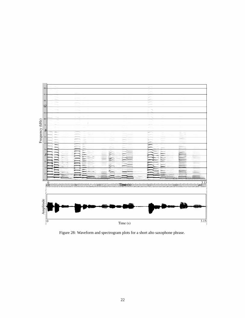
Figure 28 shows the waveform and spectrogram for amildly ambient recording of a solo alto saxophone phraseplayed by C. Potter [23]. The nineteen notes in the

phrase span the pitches G3 (G below middle C, approxi-mately 196 Hz fundamental frequency) to B flat 4 (B flatabove middle C, approximately 466 Hz fundamental fre-quency), and a wide range of dynamics. The phrase isdivided into five legato subphrases (of three, three, five,four, and three notes, respectively), each having a sharp,tongued attack on the first note.

The saxophone phrase was modeled by reassignedbandwidth-enhanced analysis data produced using a45 ms Kaiser analysis window with 90 dB sidelobe re-jection. The partials were constrained to be separatedby at least 90 Hz, less than 50% of the harmonic partialspacing for the lowest pitch in the phrase. The narrowpartial spacing is necessary to allow the notes to rever-berate without being truncated at the next attack.

Reconstructions from non-bandwidth-enhanced datalack the ambience of the original, an audible effect notclearly visible in waveform or spectrum plots. Thetongued attacks at the first note of each subphrase aresmeared in reconstructions from nonreassigned analysisdata.

A.7 Piano and Soprano Saxophone Duet

An excerpt from a recording of a duet played by J. Lo-vano, soprano saxophone, and G. Rubalcaba, piano [24],

17

Time (s)

Am

plitu

de

0 6.7

Time (s)

Freq

uenc

y (k

Hz)

00

6

6.7

2

4

Figure 24: Waveform and spectrogram plot for a flutter-tongued flute tone, pitch E4 (E above middle C). Verticalstripes on the strong harmonic partials indicate modulation due to the flutter-tongue effect. Strong low-frequencycomponents are clipped and appear to have unnaturally flat amplitude envelopes due to the high gain used to makelow-amplitude high-frequency partials visible.

18

Time (s)

Am

plitu

de

0 6.7

Time (s)

Freq

uenc

y (k

Hz)

00

6

6.7

2

4

Figure 25: Waveform and spectrogram plots for a reconstruction of the flutter-tongued flute tone plotted in Figure 24,analyzed using a long window that smears out the flutter effect.

19

Time (s)

Am

plitu

de

0 1.25

Time (s)

Freq

uenc

y (k

Hz)

00

20

1.25

8

4

12

16

Figure 26: Waveform and spectrogram plots for a bongo roll.

20

Frequency (kHz)

Time

00 s

4321

5.8 s

Figure 27: 3D spectrogram plot for an orchestral gong strike. Strong low-frequency components are clipped andappear to have unnaturally flat amplitude envelopes due to the high gain used to make low-amplitude high-frequencypartials visible.

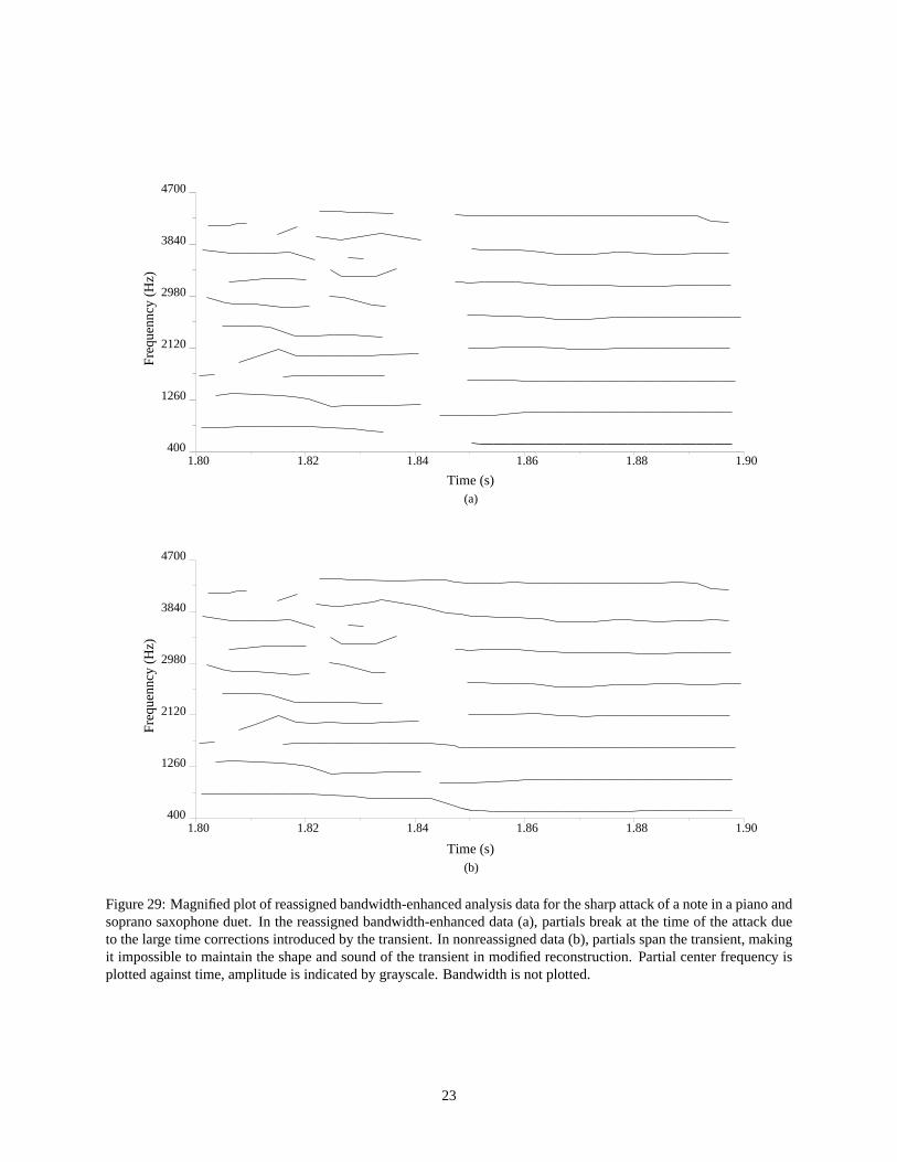
was modeled by reassigned bandwidth-enhanced anal-ysis data produced using a 24 ms Kaiser analysis win-dow with 80 dB sidelobe rejection. The ten notes in thephrase, mostly played in unison, span the pitches E4 (Eabove middle C, approximately 329 Hz fundamental fre-quency) to F5 (F above high C, approximately 698 Hzfundamental frequency). The partials were constrainedto be separated by at least 300 Hz, slightly greater than90% of the harmonic partial spacing for the lowest pitchin the phrase. All the notes articulated by the piano havesharp attacks characteristic of the piano.

The articulation of the piano is best represented by par-tials that have onsets at the time of note attacks. The par-tial breaking effect described in Section 6 is illustrated inFigure 29, which shows reassigned bandwidth-enhanced(a) and nonreassigned (b) analysis data in the vicinity ofthe unison attack of a note. Partials in the reassigneddata were broken at points having large time corrections,so that all partials have onsets at the time of the attack,rather than continuing from the decay of the previousnote.

The improvement in representation due to partial break-ing is most evident in modified (particularly time-dilated)

reconstruction. Reassigned analysis data can effectivelyreproduce unmodified transient envelopes with or with-out partial breaking, but under time-dilation, transientshape is much more effectively preserved when partialbreaking is employed.

A.8 French Speech

A speech sample is taken from a French radio an-nouncement [25, Track 2], was modeled by reassignedbandwidth-enhanced analysis data for the speech frag-ment, produced using a 39 ms Kaiser analysis windowwith 90 dB sidelobe rejection, with partials separated byat least 60 Hz. The text of the excerpt is

Le Club d’essai de la Radiodiffusion Francaisepresente un concert de bruit . . .

The speaker’s inflection introduces a variation of pitchand rhythm, visible in the magnified spectrogram plot inFigure 30, that makes this sample interesting for appli-cations of timbre morphing, spectral shaping, and cross

21

Time (s)

Am

plitu

de

0 3.15

Time (s)

Freq

uenc

y (k

Hz)

00

16

3.15

12

4

8

Figure 28: Waveform and spectrogram plots for a short alto saxophone phrase.

22

1.901.881.861.841.821.80

4700

3840

2980

2120

1260

400

1.901.881.861.841.821.80

4700

3840

2980

2120

1260

400

Time (s)

Time (s)

Freq

uenn

cy (

Hz)

Freq

uenn

cy (

Hz)

(a)

(b)

Figure 29: Magnified plot of reassigned bandwidth-enhanced analysis data for the sharp attack of a note in a piano andsoprano saxophone duet. In the reassigned bandwidth-enhanced data (a), partials break at the time of the attack dueto the large time corrections introduced by the transient. In nonreassigned data (b), partials span the transient, makingit impossible to maintain the shape and sound of the transient in modified reconstruction. Partial center frequency isplotted against time, amplitude is indicated by grayscale. Bandwidth is not plotted.

23

synthesis.

This sound proved difficult to analyze, possibly becauseof the strong low-frequency content of the low, malevoice. The fidelity of the reconstruction is quite good,but our standards are high, and the slightly reverberanttimbre makes it unsatisfying as pure speech synthesis.

References

[1] Francois Auger and Patrick Flandrin, “Improv-ing the readability of time-frequency and time-scalerepresentations by the reassignment method,”IEEETransactions on Signal Processing, vol. 43, no. 5,pp. 1068 – 1089, May 1995.

[2] Geoffroy Peeters and Xavier Rodet, “SINOLA:A new analysis/synthesis method using spectrumpeak shape distortion, phase and reassigned spec-trum,” in Proc. ICMC, 1999, pp. 153 – 156.

[3] Robert J. McAulay and Thomas F. Quatieri,“Speech analysis/synthesis based on a sinusoidalrepresentation,”IEEE Transactions on Acoustics,Speech, and Signal Processing, vol. ASSP-34, no.4, pp. 744 – 754, Aug. 1986.

[4] Xavier Serra and Julius O. Smith, “Spectral mod-eling synthesis: A sound analysis/synthesis systembased on a deterministic plus stochastic decompo-sition,” Computer Music Journal, vol. 14, no. 4, pp.12 – 24, 1990.

[5] Kelly Fitz and Lippold Haken, “Sinusoidal mod-eling and manipulation using Lemur,”ComputerMusic Journal, vol. 20, no. 4, pp. 44 – 59, 1996.

[6] Kelly Fitz, Lippold Haken, and Paul Christensen,“A new algorithm for bandwidth association inbandwidth-enhanced additive sound modeling,” inProc. ICMC, 2000.

[7] Kelly Fitz and Lippold Haken, “Bandwidth en-hanced sinusoidal modeling in Lemur,” inProc.ICMC, 1995, pp. 154 – 157.

[8] Mark Dolson, “The phase vocoder: A tutorial,”Computer Music Journal, vol. 10, no. 4, pp. 14 –27, 1986.

[9] Kunihiko Kodera, Roger Gendrin, and Claudede Villedary, “Analysis of time-varying signalswith small BT values,” IEEE Transactions onAcoustics, Speech and Signal Processing, vol.ASSP-26, no. 1, pp. 64 – 76, Feb. 1978.

[10] F. Plante, G. Meyer, and W. A. Ainsworth, “Im-provement or speech spectrogram accuracy by themethod of spectral reassignment,”IEEE Transac-tions on Speech and Audio Processing, vol. 6, no.3, pp. 282 – 287, May 1998.

[11] Kelly Fitz, Lippold Haken, and Paul Christensen,“Transient preservation under transformation in anadditive sound model,” inProc. ICMC, 2000.

[12] Tony S. Verma and Teresa H. Y. Meng, “An anal-ysis/synthesis tool for transient signals,” inProc.16th International Congress on Acoustics/135thMeeting of the Acoustical Society of America, June1998, vol. 1, pp. 77 – 78.

[13] Lippold Haken, Kelly Fitz, and Paul Christensen,“Beyond traditional sampling synthesis: Real-timetimbre morphing using additive synthesis,” inSound Of Music: Analysis, Synthesis, And Percep-tion, James W. Beauchamp, Ed. Springer-Verlag, toappear.

[14] Lippold Haken, Ed Tellman, and Patrick Wolfe,“An indiscrete music keyboard,”Computer MusicJournal, vol. 22, no. 1, pp. 30 – 48, 1998.

[15] Thomas F. Quatieri, R. B. Dunn, and T. E. Hanna,“Time-scale modification of complex acoustic sig-nals,” in Proceedings of the International Confer-ence on Acoustics, Speech, and Signal Processing.IEEE, 1993, pp. I–213 – I–216.

[16] Yinong Ding and Xiaoshu Qian, “Processingof musical tones using a combined quadraticpolynomial-phase sinusoidal and residual(QUASAR) signal model,” Journal of theAudio Engineering Society, vol. 45, no. 7/8, pp.571 – 584, July/August 1997.

[17] Kurt Hebel and Carla Scaletti, “A framework forthe design, development, and delivery of real-timesoftware-based sound synthesis and processing al-gorithms,” Audio Engineering Society Preprint,vol. A-3, no. 3874, 1994.

[18] Lippold Haken, “Computational methods forreal-time fourier synthesis,” IEEE Transactionson Acoustics, Speech and Signal Processing, vol.ASSP-40, no. 9, pp. 2327 – 2329, 1992.

[19] Kelly Fitz and Lippold Haken, “The Loris C++class library,” Available on the world wide web athttp://www.cerlsoundgroup.org/Loris.

[20] Alberto Ricci,SoundMaker 1.0.3, MicroMat Com-puter Systems, 1996-97.

24

Time (s)

Freq

uenc

y (k

Hz)

00

3

4.5

1

2

Figure 30: Spectrogram plot for a fragment of French speech magnified to show the pitch variation due to the speaker’sinflection.

[21] Frank Opolko and Joel Wapnick,McGill Univer-sity Master Samples, McGill University, Montreal,Quebec, Canada, 1987.

[22] Edwin Tellman, cello tones recorded by PatrickWolfe at Pogo Studios, Champaign IL, Jan. 1997.

[23] Chris Potter, “You and the Night and the Music,”in Concentric Circles. Concord Jazz, Inc., 1994,Track 6.

[24] Joe Lovano and Gonzalo Rubalcaba, “Flying Col-ors,” in Flying Colors. Blue Note, 1998, Track 1.

[25] “Presentation du concert de bruits,” inPierre Scha-effer - l’œuvre musicale, vol. 4. Ina-GRM (France),1990, Speaker: Jean Toscane. Track 2.

25