On the Theory of Optimal Investment Decision the Theory of Optimal...ON THE THEORY OF OPTIMAL...

On the Theory of Optimal Investment DecisionAuthor(s): J. HirshleiferReviewed work(s):Source: Journal of Political Economy, Vol. 66, No. 4 (Aug., 1958), pp. 329-352Published by: The University of Chicago PressStable URL: http://www.jstor.org/stable/1827424 .Accessed: 16/08/2012 05:15

Your use of the JSTOR archive indicates your acceptance of the Terms & Conditions of Use, available at .http://www.jstor.org/page/info/about/policies/terms.jsp

.JSTOR is a not-for-profit service that helps scholars, researchers, and students discover, use, and build upon a wide range ofcontent in a trusted digital archive. We use information technology and tools to increase productivity and facilitate new formsof scholarship. For more information about JSTOR, please contact [email protected].

.

The University of Chicago Press is collaborating with JSTOR to digitize, preserve and extend access to Journalof Political Economy.

http://www.jstor.org

http://www.jstor.org/action/showPublisher?publisherCode=ucpress

http://www.jstor.org/stable/1827424?origin=JSTOR-pdf

http://www.jstor.org/page/info/about/policies/terms.jsp

ON THE THEORY OF OPTIMAL INVESTMENT DECISION'

J. HIRSHLEIFER

University of Chicago

HIS article is an attempt to solve (in the theoretical sense), through the use of isoquant analysis, the

problem of optimal investment decisions (in business parlance, the problem of capital budgeting). The initial section re- views the principles laid down in Irving Fisher's justly famous works on interest2 to see what light they shed oil two competing rules of behavior currently proposed by economists to guide business investment decisions-the present-value rule and the internal-rate-of-return rule. The next concern of the paper is to show how Fisher's principles must be adapted when the perfect capital market assumed in his analysis does not exist- in particular, when borrowing and lending rates diverge, when capital can be secured only at an increasing marginal borrowing rate, and when capital is "ra- tioned." In connection with this last situation, certain non-Fisherian views (in particular, those of Scitovsky and of the Lutzes) about the correct ultimate goal or criterion for investment decisions are examined. Section III, which presents the solution for multiperiod investments, corrects an error by Fisher which has been the source of much difficulty. The main burden of the analysis justifies the contentions of those who reject the in-

ternal rate of return as an investment criterion, and the paper attempts to show where the error in that concept (as ordinarily defined) lies and how the internal rate must be redefined if it is to be used as a reliable guide. On the positive side, the analysis provides some support for the use of the present-value rule but shows that even that rule is at best only a partial indicator of optimal investments and, in fact, under some conditions, gives an incorrect result.

More recent works on investment decisions, I shall argue, suffer from the neg- lect of Fisher's great contributions-the attainment of an optimum through balancing consumption alternatives over time and the clear distinction between production opportunities and exchange opportunities. It is an implication of this analysis, though it cannot be pursued here in detail, that solutions to the problem of investment decision recently proposed by Boulding, Samuelson, Scitov- sky, and the Lutzes are at least in part erroneous. Their common error lay in searching for a rule or formula which would indicate optimal investment decisions independently of consumption decisions. No such search can succeed, if Fisher's analysis is sound which re- gards investment as not an end in itself but rather a process for distributing consumption over time.

The present paper deals throughout with a highly simplified situation in which the costs and returns of alternative individual investments are known with certainty, the problem being to select the scale and the mix of invest-

1 I should like to express indebtedness to many of my colleagues, and especially to James H. Lorie and Martin J. Bailey, for valuable suggestions and criticisms.

2 Irving Fisher, The Theory of Interest (New York: Macmillan Co., 1930), is most widely known. His earlier work, The Rate of Interest (New York: Macmillan Co., 1907), contains most of the essential ideas.

329

330 J. HIRSHLEIFER

ments to be undertaken. To begin with, the analysis will be limited to investment decisions relating to two time periods only. We shall see in later sections that the two-period analysis can be trans- lated immediately to the analysis of investments in perpetuities. For more general fluctuating income streams, however, additional difficulties arise whose resolution involves important new ques-

K1

V- T\

Sv \\

o~~~~~~~~~~~~

o Q P K0

FIG. 1.-Fisher's solution

tions of principle. The restriction of the solution to perfect-information situations is, of course, unfortunate, since ignorance and uncertainty are of the essence of certain important observable characteristics of investment decision behavior. The analysis of optimal decisions under conditions of certainty can be justified, however, as a first step toward a more complete theory. No further apology will be offered for considering this oversimplified problem beyond the statement that theoretical economists are in such substantial disagreement about it that a successful attempt to bring the solution within the standard body of economic doctrine would represent a real contribution.

I. TWO-PERIOD ANALYSIS

A. BORROWING RATE EQUALS LENDING

RATE (FISHER'S SOLUTION)

In order to establish the background for the difficult problems to be considered later, let us first review Fisher's solution to the problem of investment decision.3 Consider the case in which there is a given rate at which the individual (or firm)4 may borrow that is unaffected by the amount of his borrowings; a given rate at which he can lend that is unaffected by the amount of his loans; and in which these two rates are equal. These are the conditions used by Fisher; they represent a perfect capital market.

In Figure 1 the horizontal axis labeled Ko represents the amount of actual or potential income (the amount consumed or available for consumption) in period 0; the vertical axis K1 represents the amount of income in the same sense in period 1. The individual's decision problem is to choose, within the opportunities available to him, an optimum point on the graph-that is, an optimal time pattern of consumption. His starting point may conceivably be a point on either axis (initial income falling all in period 0 or all in period 1), such as points T or P, or else it may be a point in the positive quadrant (initial income falling partly in period 0 and partly in period 1), such as points W or S'. It may even lie in the second or fourth quadrants- where his initial situation involves negative income either in period 0 or in period 1.

3 Fisher's contributions to the theory of capital go beyond his solution of the problem discussed in this paper-optimal investment decision. He also considers the question of the equilibrium of the capital market, which balances the supplies and demands of all the decision-making agencies.

4 This analysis does not distinguish between individuals and firms. Firms are regarded solely as agencies or instruments of individuals.

ON THE THEORY OF OPTIMAL INVESTMENT DECISION 331

The individual is assumed to have a preference function relating income in periods 0 and 1. This preference function would be mapped in quite the ordinary way, and the curves U1 and U2 are ordinary utility-indifference curves from this map.

Finally, there are the investment opportunities open to the individual. Fisher distinguishes between "investment opportunities" and "market opportunities." The former are real productive transfers between income in one time period and in another (what we usually think of as "physical" investment, like planting a seed); the latter are transfers through borrowing or lending (which naturally are on balance off- setting in the loan market). I shall depart from Fisher's language to distinguish somewhat more clearly between "production opportunities" and "market opportunities"; the word "investment" will be used in the more general and inclusive sense to refer to both types of opportunities taken together. Thus we may invest by building a house (a sacrifice of present for future income through a production opportunity) or by lending on the money market (a sacrifice of present for future income through a market or exchange opportunity). We could, equivalently, speak of purchase and sale of capital assets instead of lending or borrowing in describing the market opportunities.

In Figure 1 an investor with a starting point at Q faces a market opportunity illustrated by the dashed line QQ'. That is, starting with all his income in time 0, he can lend at some given lending rate, sacrificing present for future income, any amount until his Ko is exhausted-re- ceiving in exchange K1 or income in period 1. Equivalently, we could say that he can buy capital assets-titles to future income Kr-with current income

Ko. Following Fisher, I shall call QQ' a "market line."5 The line PP', parallel to QQ', is the market line available to an individual whose starting point is P on the Ko axis. By our assumption that the borrowing rate is also constant and equal to the lending rate, the market line PP' is also the market opportunity to an individual whose starting point is W, within the positive quadrant.

Finally, the curve QSTV shows the range of productive opportunities available to an individual with starting point Q. It is the locus of points attainable to such an individual as he sacrifices more and more of Ko by productive investments yielding K1 in return. This attain- ability locus Fisher somewhat ambigu- ously calls the "opportunity line"; it will be called here the "productive opportunity curve" or "productive transformation curve." Note that in its concavity to the origin the curve reveals a kind of diminishing returns to investment. More specifically, productive investment projects may be considered to be ranked by the expression (AK1)/(-AKo) - 1, which might be called the "productive rate of return."6 Here AKo and AK1 represent the changes in income of periods 0 and 1 associated with the project in question.

We may conceive of whole projects being so ranked, in which case we get the average productive rate of return for each such project. Or we may rank infinitesimal increments to projects, in which case we can deal with a marginal productive rate of return. The curve QSTV will be continuous and have a

',The slope of the market line is, of course, -(1 + i), where i is the lending-borrowing rate. That is, when one gives up a dollar in period 0, he receives in exchange 1 + i dollars in period 1.

6 For the present it is best to avoid the term "internal rate of return." Fisher uses the expressions "rate of return on sacrifice" or "rate of return over cost."

332 J. HIRSHLEIFER

continuous first derivative under certain conditions relating to absence of "lumpi- ness" of individual projects (or increments to projects), which we need not go into. In any case, QSTV would represent a sequence of projects so arranged as to start with the one yielding the highest productive rate of return at the lower right and ending with the lowest rate of return encountered when the last dollar of period 0 is sacrificed at the upper left.7 It is possible to attach meaning to the portion of QSTV in the second quadrant, where Ko becomes negative. Such points could not be optimal with indifference curves as portrayed in Figure 1, of course, but they may enter into the determi- nation of an optimum. (This analysis assumes that projects are independent. Where they are not, complications ensue which will be discussed in Sections E and F below.)

As to the solution itself, the investor's objective is to climb onto as high an indifference curve as possible. Moving along the productive opportunity line QSTV, he sees that the highest indifference curve it touches is U1 at the point S. But this is not the best point attainable, for he can move along QSTV somewhat farther to the point R', which is on the market line PP'. He can now move in the reverse direction (borrowing) along PP', and the point R on the indifference curve U2 is seen to be the best attainable.

The investor has, therefore, a solution in two steps. The "productive" solution -the point at which the individual should stop making additional productive investments-is at R'. He may then move along his market line to a point better satisfying his time preferences, at R. That is to say, he makes the best in-

' An individual starting at S' would also have a "disinvestment opportunity."

vestment from the productive point of view and then "finances" it in the loan market. A very practical example is building a house and then borrowing on it through a mortgage so as to replenish current consumption income.

We may now consider, in the light of this solution, the current debate between two competing "rules" for optimal investment behavior.8 The first of these, the present-value rule, would have the individual or firm adopt all projects whose present value is positive at the market rate of interest. This would have the effect of maximizing the present value of the firm's position in terms of income in periods 0 and 1. Present value, under the present conditions, may be defined as Ko + (K1)j(1 + i), income in period 1 being discounted by the factor 1 + i, where i is the lending-borrowing rate. Since the market lines are defined by the condition that a sacrifice of one dollar in Ko yields 1 + i dollars in KI, these market lines are nothing but lines of constant present value. The equation

8 The present-value rule is the more or less standard guide supported by a great many theorists. The internal-rate-of-return rule, in the sense used here, has also been frequently proposed (see, e.g., Joel Dean, Capital Budgeting [New York: Columbia University Press, 19511, pp. 17-19). Citations on the use of alternative investment criteria may be found in Friedrich and Vera Lutz, The Theory of Investment of the Firm (Princeton, N.J.: Princeton University Press, 1951), p. 16. The internal-rate-of-return rule which we will consider in detail (i.e., adopt all projects and increments to projects for which the internal rate of return exceeds the market rate of interest) is not the same as that emphasized by the Lutzes (i.e., adopt that pattern of investments maximizing the internal rate of return). The rule considered here compares the incremental or marginal rate of return with a market rate; the other would maximize the average internal rate of return, without regard to the market rate. The latter rule will be shown to be fundamentally erroneous, even in the form the Lutzes accept as their ultimate criterion (maximize the internal rate of return on the investor's owned capital). This point will be discussed in connection with capital rationing in Sec. D, below.


for these lines is Ko + (K1)I(1 + i) = C, C being a parameter. The present- value rule tells us to invest until the highest such line is attained, which clearly takes place at the point R'. So far so good, but note that the rule says nothing about the "financing" (borrowing or lending) also necessary to attain the final optimum at R.

The internal-rate-of-return rule, in the form here considered, would have the firm adopt any project whose internal rate is greater than the market rate of interest. The internal rate for a project in the general case is defined as that discounting rate p which reduces the stream of net returns associated with the project to a present value of zero (or, equivalently, which makes the discounted value of the associated cost stream equal to the discounted value of the receipts stream). We may write

O =AKo+ ?AK + AK2+ ~p (l+ p) 2

? AKn (O + P)

In the two-period case p is identical with the productive rate of return, (AK1)j (-AKo) - 1. As in the discussion above, if infinitesimal changes are permitted, we may interpret this statement in the marginal sense. The marginal (two- period) internal rate of return is meas- ured by the slope of the productive opportunity curve minus unity. In Figure 1 at each step we would compare the steep- ness of QSTV with that of the market lines. We would move along QSTV as long as, and just so long as, it is the steeper. Evidently, this rule would have us move along QSTV until it becomes tangent to a market line at R'. Again, so far so good, but nothing is said about the borrowing or lending then necessary to attain the optimum.

At least for the two-period case, then, the present-value rule and the internal- rate-of-return rule lead to identical answers9 which are the same as that reached by our isoquant analysis, so far as productive investment decisions are concerned. The rules are both silent, however, about the market exchange between Ko and K1, which remains necessary if an optimum is to be achieved. This second step is obviously part of the solution. Had there been no actual opportunity to borrow or lend, the point S would have been the best attainable, and the process of productive investment should not have been carried as far as R'. We cannot say that the rules are definitely wrong, however, since with no such market opportunities there would have been no market rate of interest i for calculating present values or for comparison with the marginal internal rate of return. It remains to be seen whether these rules can be restated or generalized to apply to cases where a simple market rate of interest is not available for unlimited borrowing and lending. But it should be observed that, in comparison with isoquant analysis, each of the rules leads to only a partial answer.

B. WHEN BORROWING AND LENDING

RATES DIFFER

We may now depart from Fisher's analysis, or rather extend it, to a case he did not consider. The borrowing and lending rates are still assumed to be constant, independent of the amounts taken or supplied by the individual or firm under consideration. However, it is now assumed that these rates are not equal, the borrowing rate being higher than the

9 In fact, for the two-period case the rules are identical: it is possible to show that any project (or increment to a project) of positive present value must have an internal rate of return greater than the rate of interest.

334 J. HIRSHLEIFER

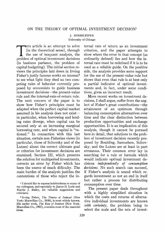
lending rate.'0 In Figure 2 there is the same preference map, of which only the isoquant U, is shown. There are now, however, two sets of market lines over the graph; the steeper (dashed) lines represent borrowing opportunities (note the direction of the arrows), and the flatter (solid) lines represent lending opportunities. The heavy solid lines show two possible sets of productive opportunities, both of which lead to solutions along U1. Starting with amount OW of Ko, an in-

K1

V~~~~~~~

0 S TV W We

FIG. 2.-Extension of Fisher's solution for differing borrowing and lending rates.

vestor with a production opportunity WVW' would move along WVW' to V, at which point he would lend to get to his time-preference optimum-the tangency with U, at V'. The curve STS' represents a much more productive possibility; starting with only OS of Ko, the investor would move along STS' to T and then borrow backward along the dashed line to get to T', the tangency point with U1. Note that the total opportunity set (the points attainable through any combina-

10 If the borrowing rate were lower than the lending rate, it would be possible to accumulate infinite wealth by borrowing and relending, so I shall not consider this possibility. Of course, financial institutions typically borrow at a lower average rate than that at which they lend, but they cannot expand their scale of operations indefinitely without changing this relationship.

tion of the market and productive opportunities) is WVV* for the first opportunity, and S'TT* for the second.

More detailed analysis, however, shows that we do not yet have the full solution-there is a third possibility. An investor with a productive opportunity locus starting on the Ko axis will never stop moving along this locus in the direction of greater K1 as long as the marginal productive rate of return is still above the borrowing rate-nor will he ever push along the locus beyond the point where the marginal productive rate of return falls below the lending rate. As- suming that some initial investments are available which have a higher productive rate of return than the borrowing rate, the investor should push along the locus until the borrowing rate is reached. If, at this point, it is possible to move up the utility hill by borrowing, productive investment should cease, and the borrowing should take place; the investor is at some point like T in Figure 2. If borrowing decreases utility, however, more productive investment is called for. Suppose investment is then carried on until diminishing returns bring the marginal productive rate of return down to the lending rate. If lending then increases utility, productive investment should halt there, and the lending take place; the investor is at some point like V in Figure 2. But suppose that now it is found that lending also decreases utility! This can only mean that a tangency of the productive opportunity locus and an indifference curve took place when the marginal productive rate of return was somewhere between the lending and the borrowing rates. In this case neither lending nor borrowing is called for, the optimum being reached directly in the productive investment decision by equating the marginal productive rate of re-


turn with the marginal rate of substitu- tion (in the sense of time preference) along the utility isoquant.

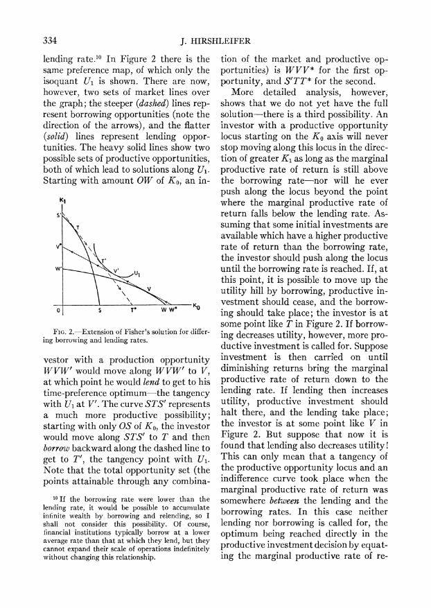
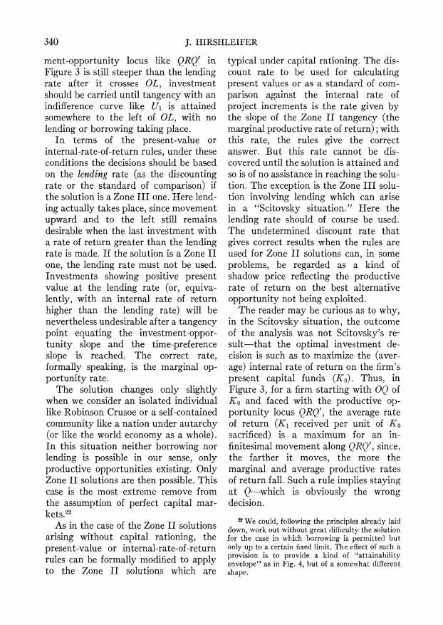
These solutions are illustrated by the division of Figure 3 into three zones. In Zone I the borrowing rate is relevant. Tangency solutions with the market line at the borrowing rate like that at T are carried back by borrowing to tangency with a utility isoquant at a point like T'. All such final solutions lie along the curve OB, which connects all points on the utility isoquants whose slope equals that of the borrowing market line. Cor- respondingly, Zone III is that zone where the productive solution involves tangency with a lending market line (like V), which is then carried forward by lending to a final tangency optimum with a utility isoquant along the line OL at a point like V'. This line connects all points on the utility isoquants with slope equal to that of the lending market line. Finally, Zone II solutions occur when a productive opportunity locus like QRQ' is steeper than the lending rate throughout Zone III but flatter than the borrowing rate throughout Zone I. Therefore, such a locus must be tangent to one of the indifference curves somewhere in Zone II.

By analogy with the discussion in the previous section, we may conclude that the borrowing rate will lead to correct answers (to the productive investment decision, neglecting the related financing question) under the present-value rule or the internal-rate-of-return rule-when the situation involves a Zone I solution. Correspondingly, the lending rate will be appropriate and lead to correct investment decisions for Zone III solutions. For Zone II solutions, however, neither will be correct. There will, in fact, be some rate between the lending and the borrowing rates which would lead to the

correct results. Formally speaking, we could describe this correct discount rate as the marginal productive opportunity rate,11 which will at equilibrium equal the marginal subjective time-preference rate. In such a case neither rule is satisfactory in the sense of providing the productive solution without reference to the utility isoquants; knowledge of the comparative slopes of the utility isoquant and the productive opportunity

K1

SI

Q, T

WI

0 S Qa W

FIG. 3.-Three solution zones for differing borrowing and lending rates.

frontier is all that is necessary, however. Of course, even when the rules in question are considered "satisfactory," they are misleading in implying that productive investment decisions can be correctly made independently of the "financing" decision.

This solution, in retrospect, may perhaps seem obvious. Where the productive opportunity, time-preference, and

11 The marginal productive opportunity rate, or marginal internal rate of return, measures the rate of return on the best alternative project. Assuming continuity, it is defined by the slope of QRQ' at R in Fig. 3. Evidently, a present-value line tangent to Ui and QRQ' at R would, in a formal sense, make the present-value rule correct. And comparing this rate with the marginal internal rate of return as it varies along QRQ' would make the internal-rate-of- return rule also correct in the same formal sense.

336 J. HIRSHLEIFER

market (or financing) opportunities stand in such relations to one another as to require borrowing to reach the optimum, the borrowing rate is the correct rate to use in the productive investment decision. The lending rate is irrelevant because the decision on the margin involves a balancing of the cost of borrowing and the return from further productive investment, both being higher than the lending rate. The lending opportunity is indeed still available, but,

K1

R

U'

wA

I ~~~~~Ki 0 Q E 0

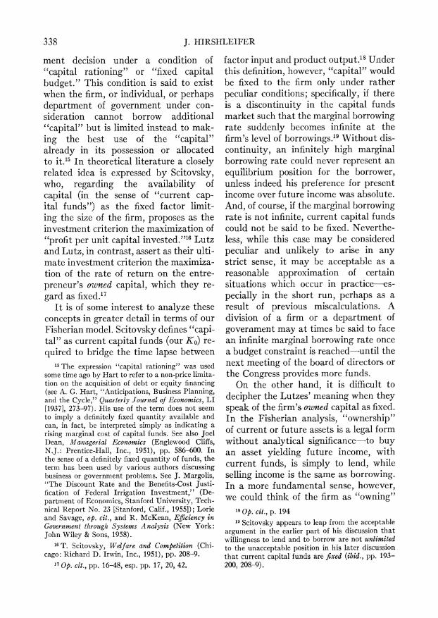
FIG. 4.-Increasing marginal cost of borrowing

the rate of return on lending being lower than the lowest marginal productive rate of return we would wish to consider in the light of the borrowing rate we must pay, lending is not a relevant alternative. Rather the relevant alternative to productive investment is a reduction in borrowing, which in terms of saving interest is more remunerative than lending. Similarly, when the balance of considerations dictates lending part of the firm's current capital funds, borrowing is not the relevant cost incurred in financing productive investment. The relevant alternative to increased productive in-

vestment is the amount of lending which must be foregone. While these considerations may be obvious, there is some disagreement in the literature as to whether the lending or the borrowing rate is the correct one.12

C. INCREASING MARGINAL COST OF BORROWING

While it is generally considered satisfactory to assume a constant lending rate (the investor does not drive down the loan rate as a consequence of his lendings), for practical reasons it is important to take account of the case in which increased borrowing can only take place at increasing cost. As it happens, however, this complication does not require any essential modification of principle.

Figure 4 shows, as before, a productive opportunity locus QR'T and an indifference curve U1. For simplicity, assume that marginal borrowing costs rise at the same rate whether the investor begins to borrow at the point R', S', or W' or at any other point along QR'T (he cannot, of course, start borrowing at Q, having no K1 to offer in exchange for more Ko). Under this assumption we can then draw market curves, now concave to the origin, like R'R, S'S, and W'W. The curve TE represents the total opportunity set as the envelope of these market curves, that is, TE connects all the points on the market curves representing the maximum Ko attainable for any given K1. By the nature of an envelope curve, TE will be tangent to a market

12The borrowing rate (the "cost of capital") has been recommended by Dean and by Lorie and Savage (see Joel Dean, Capital Budgeting [New York: Columbia University Press, 1951], esp. pp. 43-44; James H. Lorie and Leonard J. Savage, "Three Problems in Rationing Capital," Journal of Business, XXVIII [October, 1955], 229-39, esp. p. 229). Roberts and the Lutzes favor the use of the lending rate (see Friedrich and Vera Lutz, op. cit., esp. p. 22; Harry V. Roberts, "Current Problems in the Economics of Capital Budgeting," Journal of Business, XXX [January, 1957], 12-16).


curve at each such point. The optimum is then simply found where TE is tangent to the highest indifference curve attainable-here the curve U1 at R. To reach R, the investor must exploit his productive opportunity to the point R' and then borrow back along his market curve to R.

The preceding discussion applies solely to what was called a Zone I (borrowing) solution in the previous section. Depending upon the nature of the productive opportunity, a Zone II or Zone III solution would also be possible under the assumptions of this section. With regard to the present-value and the internal-rate-of-return rules, the conclusions are unchanged for Zone II and III solutions, however. Only for Zone I solutions is there any modification.

The crucial question, as always, for these rules is what rate of discount to use. Intuition tells us that the rate representing marginal borrowing cost should be used as the discount rate for Zone I solutions, since productive investment will then be carried just to the point justified by the cost of the associated increment of borrowing.'3 That is, the slope of the envelope for any point on the envelope curve (for example, R), is the same as the slope of the productive opportunity curve at the corresponding point (R') connected by the market curve.'4 If this is the case, the discount rate determined by the slope at a tangency with Ui at a point like R will also lead to productive investment being carried to R' by the rules under consideration. Of course, this again is a purely formal statement. Operationally speaking, the rules may not be of much value, since the discount

13 I should like to thank Joel Segall for insisting on this point in discussions of the problem. Note that the rate representing marginal borrowing cost is not necessarily the borrowing rate on marginal funds- an increment of borrowing may increase the rate on infra-marginal units.

rate to be used is not known in advance independently of the utility (time-preference) function.

D. RATIONING OF "CAPITAL-

A CURRENT CONTROVERSY

The previous discussion provides the key for resolving certain current disputes over what constitutes optimal invest-

14 While this point can be verified geometrically, it follows directly from the analytic properties of an envelope curve.

To simplify notation, in this note I shall denote K1 of Figure 4 as y and Ko as x. The equation of the productive opportunity locus may be written

yo= f (xo) . (a) The family of market curves can be expressed by y - yo = g(x - xo), or

F (x,xo) f + (xo) ?g(x-xo). (b)

An envelope, y = h(x), is defined by the condition that any point on it must be a point of tangency with some member of the family (b). Thus we have

h (x)= F (xxo), ( c)

dh OF (x,xo) (d) dx ax

The second condition for an envelope is that the partial derivative of the function (b) with respect to the parameter must equal zero:

oF (x,xo) =0. (e)

oxO But

OF(x,xo) d f (xo) dg (x-xo) a XO dxo 1 (x -x0)

Hence

d f (xo) dg (x-xo) dxo d(x-xo)

Also

oF (x,xo) dg (x-xo) ox d(x-xo)

So, finally,

d f (xo) dg (x-xo) OF (x,xo) d h dxo d (x-xo) dx dx

Thus the slope of the productive opportunity locus is the same as the slope of the envelope at points on the two curves connected by being on the same market curve.

338 J. HIRSHLEIFER

ment decision under a condition of "capital rationing" or "fixed capital budget." This condition is said to exist when the firm, or individual, or perhaps department of government under consideration cannot borrow additional "capital" but is limited instead to making the best use of the "capital" already in its possession or allocated to it."5 In theoretical literature a closely related idea is expressed by Scitovsky, who, regarding the availability of capital (in the sense of "current capital funds") as the fixed factor limit- ing the size of the firm, proposes as the investment criterion the maximization of "profit per unit capital invested."' Lutz and Lutz, in contrast, assert as their ultimate investment criterion the maximization of the rate of return on the entre- preneur's owned capital, which they regard as fixed.'7

It is of some interest to analyze these concepts in greater detail in terms of our Fisherian model. Scitovsky defines "capital" as current capital funds (our Ko) required to bridge the time lapse between

factor input and product output.'8 Under this definition, however, "capital" would be fixed to the firm only under rather peculiar conditions; specifically, if there is a discontinuity in the capital funds market such that the marginal borrowing rate suddenly becomes infinite at the firm's level of borrowings.'9 Without discontinuity, an infinitely high marginal borrowing rate could never represent an equilibrium position for the borrower, unless indeed his preference for present income over future income was absolute. And, of course, if the marginal borrowing rate is not infinite, current capital funds could not be said to be fixed. Neverthe- less, while this case may be considered peculiar and unlikely to arise in any strict sense, it may be acceptable as a reasonable approximation of certain situations which occur in practice-especially in the short run, perhaps as a result of previous miscalculations. A division of a firm or a department of government may at times be said to face an infinite marginal borrowing rate once a budget constraint is reached-until the next meeting of the board of directors or the Congress provides more funds.

On the other hand, it is difficult to decipher the Lutzes' meaning when they speak of the firm's owned capital as fixed. In the Fisherian analysis, "ownership" of current or future assets is a legal form without analytical significance-to buy an asset yielding future income, with current funds, is simply to lend, while selling income is the same as borrowing. In a more fundamental sense, however, we could think of the firm as "owning"

15 The expression "capital rationing" was used some time ago by Hart to refer to a non-price limita- tion on the acquisition of debt or equity financing (see A. G. Hart, "Anticipations, Business Planning, and the Cycle," Quarterly Journal of Economics, LI [19371, 273-97). His use of the term does not seem to imply a definitely fixed quantity available and can, in fact, be interpreted simply as indicating a rising marginal cost of capital funds. See also Joel Dean, Managerial Economics (Englewood Cliffs, N.J.: Prentice-Hall, Inc., 1951), pp. 586-600. In the sense of a definitely fixed quantity of funds, the term has been used by various authors discussing business or government problems. See J. Margolis, "The Discount Rate and the Benefits-Cost Justi- fication of Federal Irrigation Investment," (De- partment of Economics, Stanford University, Tech- nical Report No. 23 [Stanford, Calif., 19551); Lorie and Savage, op. cit., and R. McKean, Efficiency in Government through Systems Analysis (New York: John Wiley & Sons, 1958).

16 T. Scitovsky, Welfare and Competition (Chi- cago: Richard D. Irwin, Inc., 1951), pp. 208-9.

17 Op. cit., pp. 16-48, esp. pp. 17, 20, 42.

18 Op. cit., p. 194 19 Scitovsky appears to leap from the acceptable

argument in the earlier part of his discussion that willingness to lend and to borrow are not unlimited to the unacceptable position in his later discussion that current capital funds are fixed (ibid., pp. 193- 200, 208-9).


the opportunity set or at least the physical productive opportunities available to it, and this perhaps is what the Lutzes have in mind. Thus, Robinson Crusoe's house might be considered as his "owned capital"-a resource yielding consumption income in both present and future. The trouble is that the Lutzes seem to be thinking of "owned capital" as the value of the productive resources (in the form of capital goods) owned by the firm,20 but owned physical capital goods cannot be converted to a capital value without bringing in a rate of discount for the receipts stream. But since, as we have seen, the relevant rate of discount for a firm's decisions is not (except where a perfect capital market exists) an independent entity but is itself determined by the analysis, the capital value cannot in general be considered to be fixed independently of the investment decision.21

While space does not permit a full critique of the Lutzes' important work, it is worth mentioning that-from a Fish- erian point of view-it starts off on the wrong foot. They search first for an ultimate criterion or formula with which to

gauge investment decision rules and settle upon "maximization of the rate of return on the investor's owned capital" on what seem to be purely intuitive grounds. The Fisherian approach, in contrast, integrates investment decision with the general theory of choice-the goal being to maximize utility subject to certain opportunities and constraints. In these terms, certain formulas can be validated as useful proximate rules for some classes of problems, as I am at- tempting to show here. However, the ultimate Fisherian criterion of choice- the optimal balancing of consumption alternatives over time-cannot be reduced to any of the usual formulas.

Instead of engaging in further discussion of the various senses in which "capital" may be said to be fixed to the firm, it will be more instructive to see how the Fisherian approach solves the problem of "capital rationing." I shall use as an illustration what may be called a "Scitovsky situation," in which the investor has run against a discontinuity making the marginal borrowing rate infinite. I regard this case (which I consider empirically significant only in the short run) as the model situation under- lying the "capital rationing" discussion.

An infinite borrowing rate makes the dashed borrowing lines of Figures 2 and 3 essentially vertical. In consequence, the curve OB in Figure 3 shifts so far to the left as to make Zone I disappear for all practical purposes. There are then only Zone II and Zone III solutions. An investment-opportunity locus like WVW' in Figure 3 becomes less steep than the lending slope in Zone III, in which case the investor will carry investment up to the point V where this occurs and then lend until a tangency solution is reached at V', which would be somewhere along the curve OL of Figure 3. If an invest-

20 Lutz and Lutz, op. cit., pp. 3-13.

21 It is possible, however, that the Lutzes had in mind only the case in which an investor starts off with current funds but no other assets. In this case no discounting problems would arise in defining owned capital, so their ultimate criterion could not be criticized on that score. The objection raised below to the Scitovsky criterion, however-that it fails to consider the consumption alternative, which is really the heart of the question of investment decision-would then apply to the Lutzes' rule. In addition, a rule for an investor owning solely current funds is hardly of general enough applicability to be an ultimate criterion. The Lutzes themselves recog- nize the case of an investor owning no "capital" but using only borrowed funds, and for this case they themselves abandon their ultimate criterion (ibid., p. 42, n. 32). The most general case, of course, is that of an investor with a productive opportunity set capable of yielding him alternative combinations of present and future income.

340 J. HIRSHLEIFER

ment-opportunity locus like QRQ' in Figure 3 is still steeper than the lending rate after it crosses OL, investment should be carried until tangency with an indifference curve like U1 is attained somewhere to the left of OL, with no lending or borrowing taking place.

In terms of the present-value or internal-rate-of-return rules, under these conditions the decisions should be based on the lending rate (as the discounting rate or the standard of comparison) if the solution is a Zone III one. Here lending actually takes place, since movement upward and to the left still remains desirable when the last investment with a rate of return greater than the lending rate is made. If the solution is a Zone II one, the lending rate must not be used. Investments showing positive present value at the lending rate (or, equivalently, with an internal rate of return higher than the lending rate) will be nevertheless undesirable after a tangency point equating the investment-opportunity slope and the time-preference slope is reached. The correct rate, formally speaking, is the marginal opportunity rate.

The solution changes only slightly when we consider an isolated individual like Robinson Crusoe or a self-contained community like a nation under autarchy (or like the world economy as a whole). In this situation neither borrowing nor lending is possible in our sense, only productive opportunities existing. Only Zone II solutions are then possible. This case is the most extreme remove from the assumption of perfect capital mar- kets.22

As in the case of the Zone II solutions arising without capital rationing, the present-value or internal-rate-of-return rules can be formally modified to apply to the Zone II solutions which are

typical under capital rationing. The discount rate to be used for calculating present values or as a standard of comparison against the internal rate of project increments is the rate given by the slope of the Zone II tangency (the marginal productive rate of return); with this rate, the rules give the correct answer. But this rate cannot be dis- covered until the solution is attained and so is of no assistance in reaching the solution. The exception is the Zone III solution involving lending which can arise in a "Scitovsky situation." Here the lending rate should of course be used. The undetermined discount rate that gives correct results when the rules are used for Zone II solutions can, in some problems, be regarded as a kind of shadow price reflecting the productive rate of return on the best alternative opportunity not being exploited.

The reader may be curious as to why, in the Scitovsky situation, the outcome of the analysis was not Scitovsky's result-that the optimal investment decision is such as to maximize the (average) internal rate of return on the firm's present capital funds (Ko). Thus, in Figure 3, for a firm starting with OQ of Ko and faced with the productive opportunity locus QRQ', the average rate of return (K1 received per unit of Ko sacrificed) is a maximum for an infinitesimal movement along QRQ', since, the farther it moves, the more the marginal and average productive rates of return fall. Such a rule implies staying at Q-which is obviously the wrong decision.

22 We could, following the principles already laid down, work out without great difficulty the solution for the case in which borrowing is permitted but only up to a certain fixed limit. The effect of such a provision is to provide a kind of attainabilityy envelope" as in Fig. 4, but of a somewhat different shape.


How does this square with Scitovsky's intuitively plausible argument that the firm always seeks to maximize its returns on the fixed factor, present capital funds being assumed here to be fixed?23 The answer is that this argument is applicable only for a factor "fixed" in the sense of no alternative uses. Here present capital funds Ko are assumed to be fixed, but not in the sense Scitovsky must have had in mind. The concept here is that no additional borrowing can take place, but the possibility of consuming the present funds as an alternative to investing them is recognized. For Scitovsky, however, the funds must be invested. If in fact current income Ko had no uses other than conversion into future income K1 (this amounts to absolute preference for future over current income), Scitovsky's rule would correctly tell us to pick that point on the K1 axis which is the highest.24 Actually, our time preferences are more balanced; there is an alternative use (consumption) for Ko. Therefore, even in Scitovsky situations, we will balance Ko and K1 on the margin-and not simply accept the maximum K1 we can get in exchange for all our "fixed" Ko.25 The analyses of Scitovsky, the Lutzes, and many other recent writers frequently lead to incorrect solutions because of

their failure to take into account the alternative consumption opportunities which Fisher integrated into his theory of investment decision.

E. NON-INDEPENDENT INVESTMENT

OPPORTUNITIES

Up to this point, following Fisher, investment opportunities have been assumed to be independent so that it is possible to rank them in any desired way. In particular, they were ordered in

V~x

T1 U1

K~~~~~~ x~T'

0 Q K0

FIG. 5.-Non-independent investment opportunities-two alternative productive investment loci.

Figures 1 through 4 in terms of decreas- ing productive rate of return; the re- sultant concavity produced unique tangency solutions with the utility or market curves. But suppose, now, that there are two mutually exclusive sets of such investment opportunities. Thus we may consider building a factQry in the East or the West, but not both-contemplating the alternatives, the eastern opportunities may look like the locus QI'V, and the western opportunities like QT'T in Figure 5.26

Which is better? Actually, the solutions continue to follow directly from Fisher's principles, though too much non- independence makes for troublesome cal- culations in practice, and in some classes

26 It would, of course, reduce matters to their former simplicity if one of the loci lay completely within the other, in which case it would be obviously inferior and could be dropped from consideration.

23 Op. cit., p. 209.

24 That is, the point Q' in Fig. 3. This result is of course trivial. Scitovsky may possibly have in mind choice among non-independent sets of investments (discussed in the next section), where each set may have a different intersection with the K1 axis. Here a non-trivial choice could be made with the criterion of maximizing the average rate of return.

25 Scitovsky may have in mind a situation in which a certain fraction of current funds Ko are set apart from consumption (on some unknown basis) to become the "fixed" current capital funds. In this case the Scitovsky rule would lead to the correct result if it happened that just so much "fixed" capital funds were allocated to get the investor to the point R' on his productive transformation locus of Fig. 3.

342 J. HIRSHLEIFER

of cases the heretofore inerrant present- value rule fails. In the simplest case, in which there is a constant borrowing- lending rate (a perfect capital market), the curve QV'V is tangent to its highest attainable present-value line at V'- while the best point on QT'T is T'. It is only necessary to consider these, and the one attaining the higher present- value line (QT'T at T' in this case) will permit the investor to reach the highest

K,

FIG. 6.-Non-independent investment opportunities-poorer projects prerequisite to better ones.

possible indifference curve U, at R. In contrast, the internal-rate-of-return rule would locate the points T' and V' but could not discriminate between them. Where borrowing and lending rates differ, as in Figure 2 (now interpreting the productive opportunity loci of that figure as mutually exclusive alternatives), it may be necessary to compare, say, a lending solution at V with a borrowing solution at T. To find the optimum optimnorum, the indifference curves must be known (in Fig. 2 the two solutions attain the same indifference curve). Note that present value is not a reliable guide here; in fact, the present value of the solution V (=W*) at the relevant discount rate for it (the lending rate) far exceeds that of the solution T (= T*) at its discount rate (the borrowing rate),

when the two are actually indifferent. Assuming an increasing borrowing rate creates no new essential difficulty.

Another form of non-independence, illustrated in Figure 6, is also troublesome without modifying principle. Here the projects along the productive investment locus QQ' are not entirely independent, for we are constrained to adopt some low-return ones before certain high- return ones. Again, there is a possibility of several local optima like V and T, which can be compared along the same lines as used in the previous illustration.

F. CONCLUSION FOR TWO-PERIOD ANALYSIS

The solutions for optimal investment decisions vary according to a two-way classification of cases. The first classification refers to the way market opportunities exist for the decision-making agency; the second classification refers to the absence or presence of the complication of non-independent productive opportunities. The simplest, extreme cases for the first classification are: (a) a perfect capital market (market opportunities such that lending or borrowing in any amounts can take place at the same, fixed rate) and (b) no market opportunities whatsoever, as was true for Robinson Crusoe. Where there is a perfect capital market, the total attainable set is a tri- angle (considering only the first quadrant) like OPP' in Figure 1, just tangent to the productive opportunity locus. Where there is no capital market at all, the total attainable set is simply the productive opportunity locus itself. It is not difficult to see how the varying forms of imperfection of the capital market fit in between these extremes.

When independence of physical (productive) opportunities holds, the opportunities may be ranked in order of descending productive rate of return.


Geometrically, if the convenient (but inessential) assumption of continuity is adopted, independence means that the productive opportunity locus is every- where concave to the origin, like QS'TV in Figure 1. Non-independence may take several forms (see Figs. 5 and 6), but in each case that is not trivial non-independence means that the effective productive opportunity locus is not simply concave. This is obvious in Figure 6. In Figure 5 each of the two alternative loci considered separately is concave, but the effective locus is the scalloped outer edge of the overlapping sets of points attainable by either-that is, the effective productive opportunity locus runs along QT'T up to X and then crosses over to QV'V.

With this classification a detailed tabulation of the differing solutions could be presented; the following brief summary of the general principles involved should serve almost as well, however.

1. The internal-rate-of-return rule fails wherever there are multiple tangencies-the normal outcome for non-independent productive opportunities.

2. The present-value rule works whenever the other does and, in addition, correctly discriminates among multiple tangencies whenever a perfect capital market exists (or, by extension, whenever a unique discount rate can be determined for the comparison-for example when all the alternative tangencies occur in Zone I or else all in Zone III).

3. Both rules work only in a formal sense when the solution involves direct tangency between a productive opportunity locus and a utility isoquant, since the discount rate necessary for use of both rules is the marginal opportunity rate-a product of the analysis.

4. The cases when even the present-

value rule fails (may actually give wrong answers) all involve the comparison of multiple tangencies arising from non-independent investments when, in addition, a perfect capital market does not exist. One important example is the comparison of a tangency involving borrowing in Zone I with another involving lending in Zone III. Only reference to the utility map can give correct answers for such cases.

5. Even when one or both rules are correct in a not merely formal sense, the answer given is the "productive solution"-only part of the way toward attainment of the utility optimum. Fur- thermore, this productive decision is optimal only when it can be assumed that the associated financing decision will in fact be made.

II. A BRIEF NOTE ON PERPETUITIES

A traditional way of handling the multiperiod case in capital theory has been to consider investment decisions as choices between current funds and per- petual future income flows. For many purposes this is a valuable simplifying idea. It cannot be adopted here, however, because the essence of the practical difficulties which have arisen in multiperiod investment decisions is the reinvestment problem-the necessity of making productive or market exchanges between incomes in future time periods. In fact, the consideration of the perpetuity case is, in a sense, only a variant of the two-period analysis, in which there is a single present and a single future. In the case of perpetuity analysis, the future is stretched out, but we cannot consider transfer between different periods of the future.

All the two-period results in Section I can easily be modified to apply to the choice between current funds and per-

344 J. HIRSHLEIFER

petuities. In the figures, instead of income K1 in period 1 one may speak of an annual rate of income k. Productive opportunity loci and time-preference curves will retain their familiar shapes. The lines of constant present value (borrow-lend lines) are expressed by the equation C = Ko + (k/i) instead of C = Ko + (K1)/(1 + i). The "internal rate of return" will equal (k)/(-AKo). The rest of the analysis follows directly, but, rather than trace it out, I shall turn to the consideration of the multiperiod case in a more general way.

III. MULTIPERIOD ANALYSIS

Considerable doubt prevails on how to generalize the principles of the two- period analysis to the multiperiod case. The problems which have troubled the analysis of the multiperiod case are actually the result of inappropriate gen- eralizations of methods of solution that do lead to correct results in the simplified two-period analysis.

A. INTERNAL-RATE-OF-RETURN RULE VERSUS PRESENT-VALUE RULE

In the multiperiod analysis there is no formal difficulty in generalizing the indifference curves of Figure 1 to indifference shells in any number of dimen- sions. Also the lines of constant present value or market lines become hyper- planes with the equation (in the most general form)

Ko+K1 ? K2 ___ + 1 + il ( 1 +i O1 +i2)

+ K, _ C

(I +i1) (1 +i2) ... (I +in)

C being a parameter, i1 the discount rate between income in period 0 and 1, i2 the discount rate between periods 1 and 2,

and so forth.27 Where il = i=

in= i the expression takes on the simpler and more familiar form

_o I 1

+ K2 1 + i ( 1 + i)2

? Kn-=c ( 1 +i) n

The major difficulty with the multiperiod case turns upon the third element of the solution- the description of the productive opportunities, which may be denoted by the equation f(Ko, K1, ... * Kn) = 0. The purely theoretical speci- fication is not too difficult, however, if the assumption is made that all investment options are -independent. The problem of non-independence is not essentially different in the multiperiod case and in the two-period case, and it would enormously complicate the pres- entation to consider it here. Under this condition, then, and with appropriate continuity assumptions, the productive opportunity locus may be envisaged as a shell28 concave to the origin in all direc- tions. With these assumptions, between income in any two periods Kr and Kg

27 I shall not, in this section, consider further the possible divergences between the lending and borrowing rates studied in detail in Sec. I but shall speak simply of "the discount rate" or "the market rate." The principles involved are not essentially changed in the multiperiod case; I shall concentrate attention on certain other difficulties that appear only when more than two periods are considered. We may note that in the most general case the assumption of full information becomes rather un- realistic-e.g., that the pattern of interest rates ii through in is known today.

28 As in the two-period case, the locus represents not all the production opportunities but only the boundary of the region represented by the production opportunities. The boundary consists of those opportunities not dominated by any other; any opportunity represented by an interior point is dominated by at least one boundary point.


(holding Kt for all other periods constant) there will be a two-dimensional productive opportunity locus essentially like that in Figure 1.29

Now suppose that lending or borrowing can take place between any two suc-

cessive periods r and s at the rate is. The theoretical solution involves finding the multidimensional analogue of the point R' (in Fig. 1)-that is, the point on the highest present-value hyperplane reached by the productive opportunity locus. With simple curvature and continuity assumptions, R' will be a tangency point, thus having the additional property that, between the members of any such pair of time periods, the marginal productive rate of return between Kr and KS (holding all other K,'s constant) will be equal to the discount rate between these periods. Furthermore, if the condition is met between all pairs of successive periods, it will also be satisfied between any pairs of time periods as well.A0 Again, as in the two-period case, the final solution will involve market lending or borrowing ("financing") to move along the highest present-value hyperplane at-

29 The assumption of n-dimensional continuity is harder to swallow than two-dimensional continuity as an approximation to the nature of the real world. Nevertheless, the restriction is not essential, though it is an enormous convenience in developing the argument. One possible misinterpretation of the continuity assumption should be mentioned: it does not necessarily mean that the only investment opportunities considered are two-period options between pairs of periods in the present or future. Genuine multiperiod options are allowable-for ex- aimiple, the option described by cash-flows of -1, +4, +2, and +6 for periods 0, 1, 2, and 3, respec- tively. The continuity assumption means, rather, that if we choose to move from an option like this one in the direction of having more income in period 1 and less, say, in period 3, we can find other options available like -1, +4 + ei, +2, +6 - e3, where e, and e3 represent infinitesimals. In other words, from any point on the locus it is possible to trade continuously between incomes in any pair of periods.

30 Maximizing the Lagrangian expression C - Xf(Ko, . . , Ks), we derive the first-order conditions

oC aKo

Ic a 1+ _-X af'-0 ac 1f

aK1 1 + i) (K1 + 2) . . . (1 + i.) 1 K.

Eliminating X between any pair of successive periods:

af/OKr (1 +il) ( 1 +i2) . . .(1 +r) (1 +i8)

O f/OK8 (1 +il) (1 + i2). . . (1+ir)

(9Ks OK. - 1-fis . O9K. K2

(jos0r,s)

Between non-successive periods:

O)K, OK = (| 1 - ir+i) (1 +ir+2) . . . +(1 i-1) (1*i0)

(iXr, t)

346 J. HIRSHLEIFER

tained from the intermediate productive solution R' to the true preference optimum at R. Note that, as compared with the present value or direct solution, the principle of equating the marginal productive rate of return with the discount rate requires certain continuity assumptions.

Now it is here that Fisher, who evidently understood the true nature of the solution himself, appears to have led others astray. In his Rate of Interest he provides a mathematical proof that the optimal investment decision involves setting what is here called the marginal productive rate of return equal to the market rate of interest between any two periods.3' By obvious generalization of the result of the two-period problem, this condition is identical with that of finding the line of highest present value (the two-dimensional projection of the hyperplane of highest present value) between these time periods. Unfortunately, Fisher fails to state the qualification "between any two time-periods" consistently and at various places makes flat statements to the effect that investments will be made wherever the "rate of return on sacrifice" or "rate of return on cost" between any two options exceeds the rate of interest.32

Now the rate of return on sacrifice is, for two-period comparisons, equivalent to the productive rate of return. More generally, however, Fisher defines the rate of return on sacrifice in a multiperiod sense; that is, as that rate which reduces to a present value of zero the entire sequence of positive and negative periodic differences between the returns of any

two investment options.38 This definition is, for our purposes, equivalent to the so- called "internal rate of return.""4 This latter rate (which will be denoted p) will, however, be shown to lead to results which are, in general, not correct if the procedure is followed of adopting or re- jecting investment options on the basis of a comparison of p and the market rate."5

B. FAILURE OF THE GENERALIZED "INTERNAL

RATE OF RETURN"

Recent thinking emphasizing the internal rate of return seems to be based upon the idea of finding a purely "internal" measure of the time productivity of an investment-that is, the rate of growth of capital funds invested in a project-for comparison with the market

31 Rate of Interest, pp. 398-400. Actually, the proof refers only to successive periods, but this is an inessential restriction.

32 Ibid., p. 155; Theory of Interest, pp. 168-69.

33 Rate of Interest, p. 153; Theory of Interest, pp. 168-69.

34 For some purposes it is important to distinguish between the rate which sets the present value of a series of receipts from an investment equal to zero and that rate which does the same for the series of differences between the receipts of two alternative investment options (see A. A. Alchian, "The Rate of Interest, Fisher's Rate of Return over Cost, and Keynes' Internal Rate of Return," American Eco- nomic Review, XLV [December, 1955], 938-43). For present purposes there is no need to make the distinction because individual investment options are regarded as independent increments-so that the receipts of the option in question are in fact a sequence of differences over the alternative of not adopting that option.

35 As another complication, Fisher's mathematical analysis compares the two-period marginal rates of return on sacrifice with the interest rates between those two periods, the latter not being assumed constant throughout. In the multiperiod case Fisher nowhere states how to combine the differing period-to-period interest rates into an over-all market rate for comparison with p. It is possible that just at this point Fisher was thinking only of a rate of interest which remained constant over time, in which case the question would not arise. The difficulty in the use of the "internal rate" when variations in the market rate over time exist will be discussed below.


rate.6 But the idea of rate of growth involves a ratio and cannot be uniquely defined unless one can uniquely value initial and terminal positions. Thus the investment option characterized by the annual cash-flow sequence -1, 0, 0, 8 clearly involves a growth rate of 100 per cent (compounding annually), because it really reduces to a two-period option with intermediate compounding. Simi- larly, a savings deposit at 10 per cent compounded annually for n years may seem to be a multiperiod option, but it is properly regarded as a series of two- period options (the "growth" will take place only if at the beginning of each period the decision is taken to reinvest the capital plus interest yielded by the investment of the previous period). A savings-account option without reinvestment would be: -1, .10, .10, .10,

, ,1.10 (the last element being a termi- nating payment); with reinvestment, the option becomes-1, 0, 0, 0, . . . , (1.1.0)n, n being the number of compounding periods after the initial deposit.

Consider, however, a more general investment option characterized by the sequence - 1, 2, 1. (In general, all investment options considered here will be normalized in terms of an assumed $1.00 of initial outlay or initial receipt.) How can a rate of growth for the initial capital outlay be determined? Unlike the savings-account opportunity, no information is provided as to the rate at which the intermediate receipt or "cash throwoff" of $2.00 can be reinvested. If, of course, we use some external discounting rate (for example, the cost of capital or the rate of an outside lending opportunity), we will be departing from the idea of a purely internal growth rate. In fact, the use of an external rate will simply re-

duce us to a present-value evaluation of the investment option.

In an attempt to resolve this difficulty, one mathematical feature of the two- period marginal productive rate of return was selected for generalization by both Fisher and his successors. This feature is the fact that, when p (in the two-period case equal to the marginal productive rate of return [AK1]/[- AKo] - 1) is used for discounting the values in the receipt-outlay stream, the discounted value becomes zero. This concept lends itself to easy generalization: for any multiperiod stream there will be a similar discounting rate p which will make the discounted value equal to zero (or so it was thought). This rate seems to be purely internal, not infected by any market considerations. And, in certain simple cases, it does lead to correct answers in choosing investment projects according to the rule: Adopt the project if p is greater than the market rate r.

For the investment option - 1, 2, 1 considered above, p is equal to V/2, or 141.4 per cent. And, in fact, if the borrowing rate or the rate on the best alternative opportunity (whichever is the appropriate comparison) is less than -Vi, the investment is desirable. Figure 7 plots the present value C of the option as a function of the discounting interest rate, i, assumed to be constant over the two discounting periods. Note that the present value of the option diminishes as i increases throughout the entire relevant range of i, from i = - 1 to i = .37 The internal rate of return p is that i for which the present value curve cuts the horizontal axis. Evidently, for any i < p, present value is positive; for

37 Economic meaning may be attached to negative interest rates; these are rates of shrinkage of capital. I rule out the possibility of shrinkage rates greater than 100 per cent, however.

36 See K. E. Boulding, Economic Analysis (rev. ed.; New York: Harper & Bros., 1948), p. 819.

348 J. HIRSHLEIFER

i > p, it is negative. However, the fact that the use of p

leads to the correct decision in a particular case or a particular class of cases does not mean that it is correct in prin-

C

3

2

-1 1 2 3 4

FIG. 7.-Sketch of present value of the option -1, 2, 1.

C

Pin

FIG. 8.-Two alternative options

ciple. And, in fact, cases have been ad- duced where its use leads to incorrect answers. Alchian has shown that, in the comparison of two investment options which are alternatives, the choice of the one with a higher p is not in general correct-in fact, the decision cannot be made without knowledge of the appropriate external discounting rate.38 Figure 8 illustrates two such options, I being

preferable for low rates of interest and II for high rates. The i at which the cross- over takes place is Fisher's rate of return on sacrifice between these two options. But II has the higher internal rate of return (that is, its present value falls to zero at a higher discounting rate) regardless of the actual rate of interest. How can we say that I is preferable at low rates of interest? Because its present value is higher, it permits the investor to move along a higher hyperplane to find the utility optimum attained somewhere on that hyperplane. If IJ were adopted, the investor would also be en- abled to move along such a hyperplane, but a lower one. Put another way, with the specified low rate of interest, the investor adopting I could, if he chose, put himself in the position of adopting II by appropriate borrowings and lendings together with throwing away some of his wealth.39

Even more fundamentally, Lorie and Savage have shown that p may not be unique.40 Consider, for example, the in-

39 Some people find this so hard to believe that 1 shall provide a numerical example. For investment I, we may use the annual cash-flow stream -1, 0, 4-then the internal rate of return is 1, or 100 per cent. For investment option II, we may use the option illustrated in Figure 7: -1, 2, 1. For this investment p is equal to /2, or 141.4 per cent. So the internal rate of return is greater for II. However, the present value for option I is greater at an interest rate of 0 per cent, and in fact it remains greater until the cross-over rate, which happens to be at 50 per cent for these two options. Now it is simple to show how, adopting I, we can get to the result II at any interest rate lower than 50 per cent-10 per cent, for example. Borrowing from the final time period for the benefit of the intermediate one, we can convert -1, 0, 4 to - 1, 2.73, 1 (I have subtracted 3 from the final period, crediting the intermediate period with 3/1.1 = 2.73). We can now get to option II by throwing away the 0.73, leaving us with -1, 2, 1. The fact that we can get to option II by throwing away some wealth demonstrates the superiority of I even though Pi, > PI,

provided that borrowing and lending can take place at an interest rate less than the cross-over discounting rate of 50 per cent.

38 Alchian, op. cit., p. 939. 40 0p. cit., pp. 236-39.


vestment option -1, 5, -6. Calcula- tion reveals that this option has a present value of zero at discounting rates of both 100 per cent and 200 per cent. For this investment option present value as a function of the discounting rate is sketched in Figure 9. While Lorie and Savage speak only of "dual" internal rates of return, any number of zero values of the present-value function are possible in principle. The option - 1, 6, -11, 6, illustrated in Figure 10, has

C

-11 3 4

-21

-3

FIG. 9.-Sketch of present value of the investment option -1, 5, -6.

zero present value at the discounting rates 0 per cent, 100 per cent, and 200 per cent, for example.41

In fact, perfectly respectable investment options may have no real internal rates (the present value equation has only imaginary roots). The option -1, 3,-22 is an example; a plot would show that its present value is negative throughout the relevant range.42 It is definitely not the case, however, that all options

-1

FIG. 10.-Sketch of present value of the investment option -1, 6, -11, 6.

for which the internal rate cannot be calculated are bad ones. If we merely reverse the signs on the option above to get 1, -3, 21, we have an option with positive present value at all rates of discount.

These instances of failure of the multiperiod internal-rate-of-return rule (note that in each case the present-value rule continues to indicate the correct answer unambiguously, setting aside the question of the appropriate discounting rate which was discussed in Sec. I) are, of course, merely the symptom of an under- lying erroneous conception. It is clear

42 Mathematically, the formula for the roots of a three-period option no, n1, n2 where no = -1 is:

(n1-2) ? Vn/2+4 4n

2

If -4n2 exceeds n2, the roots will be imaginary, and an internal rate of return cannot be calculated. A necessary condition for this result is that the sum of the undiscounted cash flows be negative, but this condition should not rule out consideration of an option (note the option -1, 5, -6 in Fig. 9).

41 The instances discussed above suggest that the alternation of signs in the receipt stream has something to do with the possibility of multiple p's. In fact, Descartes's rule of signs tells us that the number of solutions in the allowable range (the number of points where present value equals zero for i > -1) is at most equal to the number of re- versals of sign in the terms of the receipts sequence. Therefore, a two-period investment option has at most a single p, a three-period option at most a dual p, and so forth. There is an interesting footnote in Fisher which suggests th4t he was not entirely unaware of this difficulty. Where more than a single-sign alternation takes place, he suggests the use of the present-value method rather than at- tempting to compute "the rate of return on sacrifice" (Rate of Interest, p. 155). That any number of zeros of the present value function can occur was pointed out by Paul A. Samuelson in "Some Aspects of the Pure Theory of Capital," Quarterly Journal of Economics, LI (1936-37), 469-96 (at p. 475).

350 J. HIRSHLEIFER

that the idea that p represents a growth rate in any simple sense cannot be true; a capital investment of $1.00 cannot grow at a rate both of 100 per cent and of 200 per cent. Even more fundamentally, the idea that p is a purely internal rate is not true either. Consider the option -1, 2, 1 discussed earlier, with a unique p equal to V. The intermediate cash throwoff of $2.00 must clearly be reinvested externally of this option. How does the calculation of p handle this? This answer is that the mathematical manipulations involved in the calculation of p implicitly assume that all intermediate receipts, positive or negative, are treated as if they could be compounded at the rate p being solved for.43 The rate p has been characterized rather appropriately as the "solving rate" of interest. But note that this mathematical manipulation, even where it does lead to a unique answer (and, in general, it will not), is unreason- able in its economic implications. There will not normally be other investment opportunities arising for investment of intermediate cash proceeds at the rate p, nor is it generally true that intermediate cash inflows (if required) must be obtained by borrowing at the rate p. The rate p, arising from a mathematical manipulation, will only by rare coinci- dence represent relevant economic alternatives.

The preceding arguments against the use of the usual concept of the "internal rate of return" do not take any account of the possibility of non-constant interest rates over time. Martin J. Bailey has emphasized to me that it is precisely when this occurs (when there exists a

known pattern of future variation of i) that the internal-rate-of-return rule fails most fundamentally. For in the use of that rule all time periods are treated on a par; the only discounting is via the solving rate defined only in terms of the sequence of cash flows. But with (a known pattern of) varying future i, shifts in the relative desirability of income in different periods are brought about. In the usual formulation the internal rate of return concept can take no account of this. In fact, in such a case one might have an investment for which p was well defined and unique and still not be able to de- termine the desirability of the investment opportunity (that is, depending upon the time pattern of future interest rates, present value might be either negative or positive).

The following remarks attempt to summarize the basic principles discussed in this section.

At least in the simplest case, where we do not worry about differences between borrowing and lending rates but assume these to be equal and also constant (constant with respect to the amount borrowed or lent-not constant over time), the multidimensional solution using the present-value rule is a straightforward generalization of the two-period solution. The principle is to push productive investment to the point where the highest attainable level of present value is reached and then to "finance" this investment by borrowing or lending between time periods to achieve a time- preference optimum.

The main burden of these remarks has been to the effect that the internal-rate- of-return rule, unlike the present-value rule, does not generalize to the multiperiod case if the usual definition of the internal rate p is adopted-that is, as that rate which sets the present value of

43 The true significance of the reinvestment assumption was brought out in Ezra Solomon, "The Arithmetic of Capital-budgeting Decisions," Journal of Business, XXIX (April, 1956), 124-29, esp. pp. 126-27.


the discounted income stream equal to zero. I have tried to show the multiperiod generalization which would make the internal-rate-of-return rule still correct: between every pair of time periods, the marginal internal rate of return in the sense of the marginal productive rate of return between those two periods, holding income in other periods constant, should be set equal to the market discount rate between those periods. That the usual interpretation of the internal- rate-of-return rule is not in general correct has been illustrated by its failure in particular cases and has been explained by exposing the implicit assumption made in the mathematical manipulation which finds p- that all intermediate cash flows are reinvested (or borrowed, if cash flows are negative) at the rate p itself. In addition, p does not allow for varying interperiod preference rates (or interest rates) over time. This generalized multiperiod internal rate of return is, therefore, not really internal, nor is the assumption implied about the external opportunities generally correct or even generally reasonable.

IV. CONCLUDING COMMENTS

The preceding analysis has slighted a great many questions. In addition, lack of time has precluded comparative discussion of the works of other authors, however helpful this might have been.44

I have not attempted to generalize the results to the multiperiod case with non- independent investments or with differing or non-constant borrowing and lending rates. On the latter points intuition suggests that whether the borrowing or lending rate in calculating present value is to be used for any time period does not depend upon any characteristics of the investment option under consideration in isolation; it depends rather upon

the over-all cash position after adoption of that option as an increment. If, after such adoption, time preference dictates shifting to less income in period r and more in period t, any income associated with the option in question falling in period r should be discounted back to the next earlier period at the lending rate (and that for period t at the borrowing rate). Income in any period s may then have been successively discounted at borrowing rates for a number of periods and lending rates for a number of others before being reduced to a present value.

The main positive conclusion of the paper is that the present-value rule for investment decisions is correct in a wide variety of cases (though not universally) and in a limited sense. The rule tells us to attain the highest possible level of present value, but the point at which this condition is satisfied (that is, the distribution of incomes in various time periods) is not the final solution. It is, rather, an intermediate "productive" solution which must then be modified by borrowing or lending ("financing") to find the over-all optimum. This becomes particularly clear when we consider the case where lending and borrowing rates differ and thus enter the subcontroversy

44I should comment, though, on the important article by Samuelson, op. cit. The results here are in part consistent with his, with the following main differences: (1) He limits himself to the analysis of a single investment, whereas I consider the entire investment-consumption pattern over time. (2) He concludes in favor of the present-value rule, discounting at the market rate of interest. I have attempted to consider explicitly the problem of what to do when the borrowing and lending rates diverge, or vary as a function of the amount borrowed, and I do not find the present-value rule to be universally valid. Of these differences, the first is really crucial. It is the heart of Fisher's message that investments cannot be considered in isolation but only in the context of the other investment and consumption alternatives available. Nevertheless, Samuelson's article suffices to refute a number of fallacies still current in this field of economic theory.

352 J. HIRSHLEIFER

between those who favor the use of present-value discounting at the cost of capital and those who would discount at the alternative lending rate. Which is correct depends upon the financing necessary to approach the time-preference optimum. Furthermore, if a tangency takes place between the productive opportunity locus and the time-preference utility isoquant at a rate between the lending and the borrowing rates, the "productive" solution requires no financing and the present-value principle is only correct in a formal sense. The present-value rule fails to give correct answers only for certain cases which combine the difficulties of non-independent investments and absence of a perfect capital market. When a perfect capital market exists, the present-value rule is universally correct in the limited sense referred to above. With independent investments but an imperfect capital market, the present-value rule will give answers which are correct but possibly only in a formal sense (the discounting rate used is not an external opportunity but an internal shadow price which comes out of the analysis).

The main negative conclusion is that the internal-rate-of-return rule for the multiperiod case is not generally correct, if the usual definition of the internal rate is adopted as that discount rate which makes the present value of the income stream associated with an investment option equal to zero. The so-called internal rate will only give correct answers in general if restricted to two-period comparisons; I have called this two- period internal rate the productive rate of return. For multiperiod investments

the usual internal-rate-of-return rule (compare p with the market rate r) is not generally correct; however, given certain continuity assumptions, the correct answer will be arrived at by setting the marginal productive rate of return between each pair of time periods equal to the discount or market rate between those periods.

More important than the specific detailed conclusions is the demonstration that the Fisherian approach-the analysis of investment decisions as a means of balancing consumption incomes over time, together with the distinction between productive and market investment opportunities-is capable of solving (in the theoretical sense) all the problems posed. This solution is, furthermore, not an excrescence upon the general economic theory of choice but entirely integrated with it, constituting another dimension, so to speak. Since Fisher, economists working in the theory of investment decision have tended to adopt a mechanical approach-some plumping for the use of this formula, some for that. From a Fisherian point of view, we can see that none of the formulas so far propounded is universally valid. Furthermore, even where the present-value rule, for example, is correct, few realize that its validity is conditional upon making certain associated financing decisions as the Fisherian analysis demonstrates. In short, the Fisherian approach permits us to define the range of applicability and the short- comings of all the proposed formulas- thus standing over against them as the general theoretical solution to the problem of investment decision under conditions of certainty.

On the Theory of Optimal Investment Decision the Theory of Optimal...ON THE THEORY OF OPTIMAL...

Documents

Transcript of On the Theory of Optimal Investment Decision the Theory of Optimal...ON THE THEORY OF OPTIMAL...