On the Stability of Pressure Relief...

Guiding the development ofwood-based materials towards more sustainable productsExamens-/kandidatarbete inom civilingenjörsprogrammet

EMILIA EMILSSON

Department of Ckjkjk.jouhb jn kjkljjljjllökjghjCHALMERS UNIVERSITY OF TECHNOLOGYGothenburg, Sweden 2014


EMILIA EMILSSON



EMILIA EMILSSON



EMILIA EMILSSON


On the Stability of Pressure Relief ValvesA numerical study using CFDMaster’s Thesis in the Master’s program Innovative and Sustainable ChemicalEngineering

ANNA BORGSOFIA JAKOBSSONDepartment of Chemical EngineeringChalmers University of TechnologyGothenburg, Sweden 2014Master’s Thesis 2014:06

MASTER’S THESIS IN CHEMICAL ENGINEERING

On the Stability of Pressure Relief ValveA numerical study using CFD

ANNA BORG & SOFIA JAKOBSSON

Department of Chemical and Biological EngineeringDivision of Chemical Engineering

Chalmers University of TechnologyGothenburg, Sweden 2014

On the Stability of Pressure Relief ValvesA numerical study using CFDANNA BORG & SOFIA JAKOBSSON

c©ANNA BORG & SOFIA JAKOBSSON, 2014

Master’s Thesis 2014:06Department of Chemical EngineeringChalmers University of TechnologySE-412 96 GothenburgSwedenTelephone: +46 (0)31-772 1000

Chalmers Reproservice/Department of Chemical EngineeringGothenburg, Sweden 2014

Abstract

A numerical model based on a spring loaded safety relief valve on the residual heatsystem at the nuclear power plant Ringhals has been constructed with CFD usingANSYS 14.5.7. Through stationary simulations, characteristics for the valve has beenobtained and compared to the dynamic opening of the valve. The stability of the valvehas been investigated by varying the upstream conditions. It was concluded that thetransient opening of the valve with an inlet line of 0.25m can be predicted by thevalve characteristics. For systems with longer inlet lines there are transient effects thatare not captured by stationary simulations. If the inlet line is sufficiently short orsufficiently long, the valve does not exhibit unstable behavior. The numerical modelof the valve can capture the interaction between the pressure wave propagation in thesimulation and the disc position. The effect of frictional elements has been examinedby implementing a hysteresis factor to the closing of the valve. This proved to be aneffective way of attenuating chatter. For a constant inflow of mass, the disc frequencyof the oscillations was independent of the magnitude of the mass flow. The amplitudeof the oscillations, however, was not. A system with large volume had a tendency tooscillate with a lower frequency than a system of small volume.

Keywords: Stability, Pressure relief valve, CFD

i

PrefaceThis Master of Science thesis has been performed by Anna Borg and Sofia Jakobsson,students at the Master’s program Innovative and Sustainable Chemical Engineeringat Chalmers University of Technology, Gothenburg Sweden. The thesis has been per-formed in collaboration with ÅF Industry, Ringhals (Vattenfall) and the departmentof Chemical Engineering at Chalmers University of Technology. It was supervised byOscar Granberg at ÅF Industry and Daniel Edebro at Ringhals. The examiner atChalmers University of Technology was Bengt Andersson.

AcknowledgmentsWe would like to sincerely thank our supervisors Oscar Granberg and Daniel Edebrofor dedicated help regarding any problems encountered. We would also like to thankall the people at Ringhals and ÅF Industry - Technical Analysis, for their welcomingand interest in this thesis.

Anna Borg & Sofia Jakobsson, Gothenburg 2014-06-03

ii

Contents

1 Introduction 1

1.1 Objective . . . . . . . . . . . . . . . . . . . . . . . . . . . . . . . . . . 1

1.2 Constraints . . . . . . . . . . . . . . . . . . . . . . . . . . . . . . . . . 1

1.3 Method . . . . . . . . . . . . . . . . . . . . . . . . . . . . . . . . . . . 2

2 Background 3

2.1 Safety valves . . . . . . . . . . . . . . . . . . . . . . . . . . . . . . . . . 3

2.2 Design Standards . . . . . . . . . . . . . . . . . . . . . . . . . . . . . . 6

2.3 Popping or proportional valves . . . . . . . . . . . . . . . . . . . . . . . 6

2.4 Safety valve instabilities . . . . . . . . . . . . . . . . . . . . . . . . . . 7

2.5 Relieving Transients . . . . . . . . . . . . . . . . . . . . . . . . . . . . 7

2.6 Previous work . . . . . . . . . . . . . . . . . . . . . . . . . . . . . . . . 8

3 Physics 12

3.1 Pressure wave . . . . . . . . . . . . . . . . . . . . . . . . . . . . . . . . 12

3.2 Inertia . . . . . . . . . . . . . . . . . . . . . . . . . . . . . . . . . . . . 13

3.3 Forces acting on the disc . . . . . . . . . . . . . . . . . . . . . . . . . . 14

3.4 Forces considered in this thesis . . . . . . . . . . . . . . . . . . . . . . . 15

4 Valve characteristics 16

5 Hypotheses about valve characteristics and stability 21

iii

5.1 Valve characteristics . . . . . . . . . . . . . . . . . . . . . . . . . . . . 21

5.2 Stability . . . . . . . . . . . . . . . . . . . . . . . . . . . . . . . . . . . 22

6 Numerical model 27

6.1 Governing equations . . . . . . . . . . . . . . . . . . . . . . . . . . . . 27

6.2 Mesh and geometry . . . . . . . . . . . . . . . . . . . . . . . . . . . . . 29

6.3 Dynamic mesh and UDF . . . . . . . . . . . . . . . . . . . . . . . . . . 30

6.4 Simulations . . . . . . . . . . . . . . . . . . . . . . . . . . . . . . . . . 31

6.5 Sensitivity analysis . . . . . . . . . . . . . . . . . . . . . . . . . . . . . 35

7 Numerical results 38

7.1 Constant pressure . . . . . . . . . . . . . . . . . . . . . . . . . . . . . . 38

7.2 Constant mass flow . . . . . . . . . . . . . . . . . . . . . . . . . . . . . 51

8 Analysis and Discussion 54

9 Conclusions 58

10 Further work 59

Appendices 60

A Cavitation 61

A.1 Theory . . . . . . . . . . . . . . . . . . . . . . . . . . . . . . . . . . . . 61

A.2 Modelling cavitation . . . . . . . . . . . . . . . . . . . . . . . . . . . . 62

A.3 Results . . . . . . . . . . . . . . . . . . . . . . . . . . . . . . . . . . . . 63

A.4 Analysis . . . . . . . . . . . . . . . . . . . . . . . . . . . . . . . . . . . 65

B Orifice area 66

C Numerical settings in FLUENT 67

iv

C.1 Turbulence model and boundary conditions . . . . . . . . . . . . . . . . 67

C.2 Calculation schemes . . . . . . . . . . . . . . . . . . . . . . . . . . . . 67

C.3 Additional settings . . . . . . . . . . . . . . . . . . . . . . . . . . . . . 67

C.4 Convergence . . . . . . . . . . . . . . . . . . . . . . . . . . . . . . . . . 69

v

1. Introduction

A safety valve protects a system from elevated pressures by discharging the pressuremedia. Safety valves are thus an important part of all types of industries and theirwell-functioning is of great importance since they often are the last resort to preventaccidents. There are a number of different properties of the safety valve and the systemto which it is attached to that are thought to affect the response of the valve. Byexamining the effect of different system properties, their importance for the valve sta-bility might be established and unstable valve behavior might be prevented. It is alsoof interest to create a simple tool that can be used to assess whether or not a certainvalve will operate stable prior to installation.

1.1 ObjectiveThe first objective of this thesis is to investigate if steady-state characteristics canbe used to make a first estimation of the opening behavior of a valve. The secondobjective is to study a number of system variables and evaluate their influence on thevalve stability. Pressure drop over the inlet piping, different pipe lengths and differentvolumes of the valve system are features that will be examined. Safety valves can bedamped by friction to prevent unstable operation, the effect of friction hysteresis will beexamined. Safety relief valves can be proportional with high-lifting regions or popping,further in this thesis it will be investigated whether a valve itself can be characterizedas any of these categories or if it is the system to which it belongs that determine thebehavior of the valve.

1.2 Constraints

1.2.1 General constraints

• All tests will be executed with a numerical model based on an existing pressurerelief valve.

• The model does not aim at completely replicating an actual valve behavior.

• Only effects generated by the preceding system will be investigated.

1

1.2.2 Model constraints

• The entire domain is filled with water as initial conditions of the simulations.

• The temperature of the fluid is constant, 298K.

• Axisymmetric 2D-model.

• Only modeling fluid and rigid body motion.

• The modeled valve is bellowed and the back pressure is 1 atm.

1.3 MethodThe safety relief valve was simulated with ANSYS Fluent v14.5. The geometries wheredrawn in DesignModeler and the mesh was created in ANSYS Meshing. Steady statecharacteristics were created with a 2-dimensional geometry and compared to transientsimulations. The transient simulations were also performed in 2-dimensions in orderto investigate the transient response of the valve to varying inlet pipe length, discretepressure drop and variable system volume. The transient simulations were conductedwith a gradual increase of inlet pressure or inlet velocity. Further, a sensitivity analysisto validate the accuracy of the simulations was also performed.

2

2. Background

This chapter will explain the basics behind safety valves and their operation. Theconcept of valve characteristics will be introduced and explained along with the clas-sification of safety valves based on their opening behavior. Last, a part of the designstandards regarding safety valve issued by ASME will be presented. The conceptspresented in this section/chapter will be used throughout the rest of the thesis.

2.1 Safety valvesSafety relief valves are used in all kinds of industries. Their task is to protect the systemfrom elevated pressures that may result in damage to equipment and operators. Safetyrelief valves are designed to respond to the pressure in the system and are completelyautomatic, that is, no external signal from an operator or regulator is required for thevalve to open.

A simple way to describe a safety relief valve is to imagine a disc/weight placed hori-zontally on a (pipe) opening. When the pressure in the pipe is high enough, the discwill be pushed from its position, allowing for the media inside the pipe to flow out.The safety valve considered in this thesis is spring-loaded which means that the discis pressed to the opening by a spring. The spring can be tensioned to yield differentopening pressures for the valve. Increasing the spring tension also increases the pressurerequired to lift the disc and open the valve. Figure 2.1 shows a spring-loaded safetyvalve.

3

Det

ta ä

r dok

umen

t 317

1261

, Ver

sion

02

från

Rin

ghal

s DM

S-sy

stem

, D

okum

ents

tatu

s: F

R, S

tatu

sdat

um: 2

011.

12.0

5, D

okum

entk

od: A

-D-0

6-04

-R, H

andl

ägga

re: P

RN

N, S

ekre

tess

klas

s För

etag

sint

ern

Leve

rant

ören

s sek

rete

sskl

ass:

Ej b

edöm

d

Figure 2.1: Picture of a safety valve

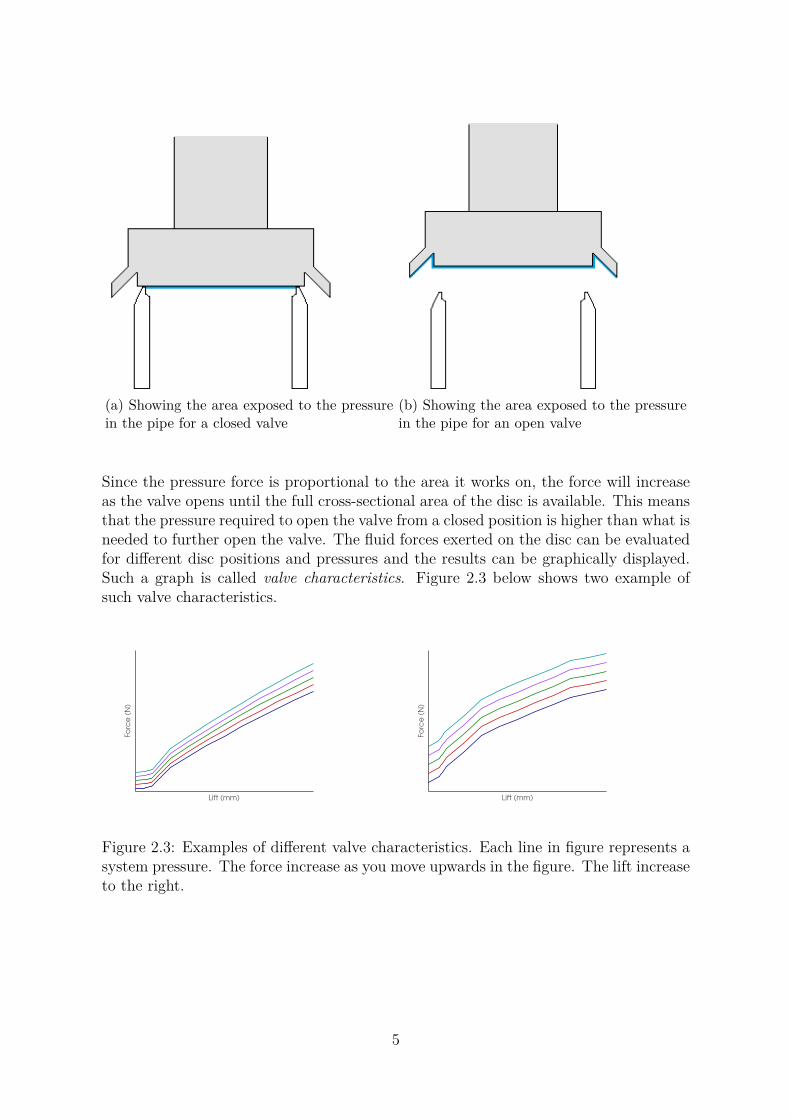
As can be seen in figure ??, the diameter of the disc is larger than the diameter ofthe pipe. This feature has an important impact on the opening behavior of the valve.When the valve is closed, the area exposed to the pressure in the pipe is the same as thecross-sectional area of the pipe, see X in figure 2.2a. As the valve opens, the exposedarea increases, see figure2.2b.

4

(a) Showing the area exposed to the pressurein the pipe for a closed valve

(b) Showing the area exposed to the pressurein the pipe for an open valve

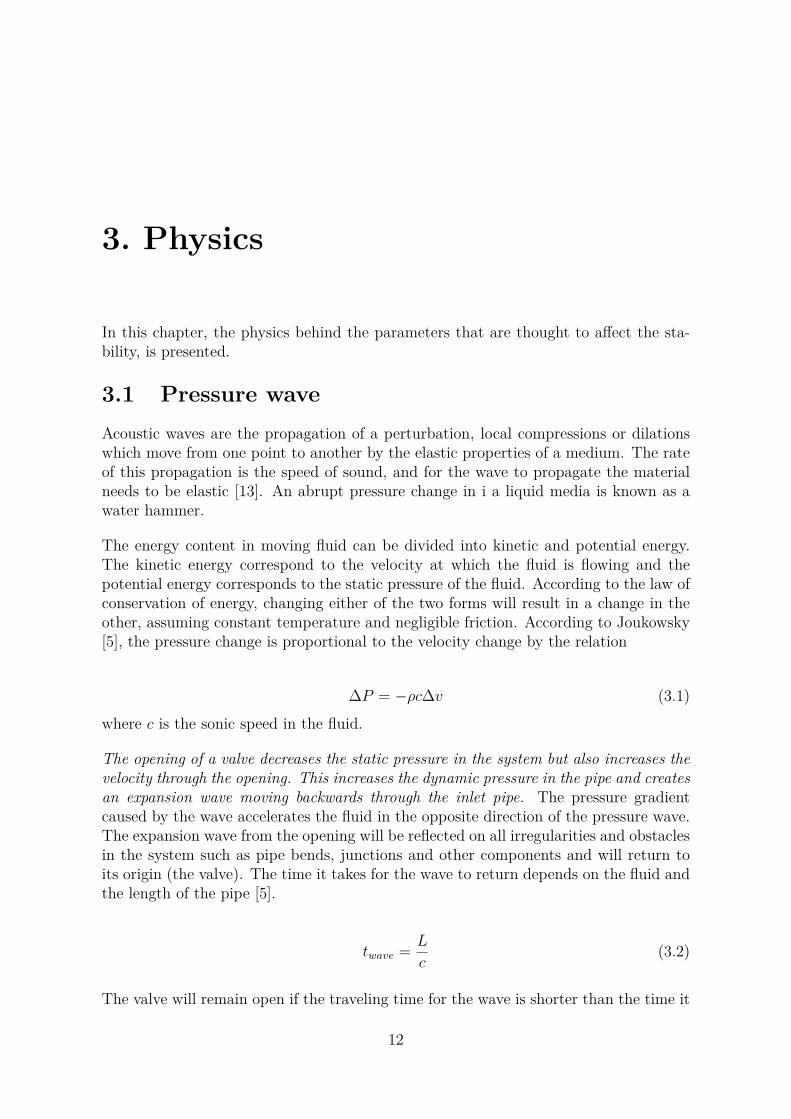
Since the pressure force is proportional to the area it works on, the force will increaseas the valve opens until the full cross-sectional area of the disc is available. This meansthat the pressure required to open the valve from a closed position is higher than what isneeded to further open the valve. The fluid forces exerted on the disc can be evaluatedfor different disc positions and pressures and the results can be graphically displayed.Such a graph is called valve characteristics. Figure 2.3 below shows two example ofsuch valve characteristics.

Lift (mm)

Fo

rce

(N

)

Lift (mm)

Fo

rce

(N

)

Figure 2.3: Examples of different valve characteristics. Each line in figure represents asystem pressure. The force increase as you move upwards in the figure. The lift increaseto the right.

5

2.2 Design StandardsTo ensure proper operation of a pressure relief valve there exists a Design standard.Some of these will be presented below to give a better idea of how a safety valve isdesigned and working. The criteria are valid for relief valves used in systems withliquid media. The following design standards are proposed by ASME to ensure a stableand reliable operation of the safety valve.

• The opening pressure, Popen, should be lower or equal to the design pressure ofthe system.

• The valve should be completely open at a pressure of 110% of the opening pressureor at a pressure 0.21 bar over the opening pressure.

• The allowed tolerance for the opening pressure in safety valves with openingpressures between 0 and 4.8 bar(g) is ±0.14 bar(g) and for opening pressures above4.8 bar(g), the tolerance is ±3%.

• The pressure drop over the inlet pipe is limited to 3% of 1.1 · Popen.

• The valve should ensure that the pressure in the system it protects never exceeds110% of the design pressure for expected transients. For unexpected transients,the pressure cannot exceed 120% of the design pressure.

2.3 Popping or proportional valvesSafety valves are often divided into proportional valves and high-lifting or poppingvalves. This categorization assumes that the valve behaves in a certain way regardlessof the system it is attached to. The same type of safety relief valve are found oninlet pipes of greatly varying length. How this affect the behavior of the valve is oftenneglected.

A popping or high-lifting behavior is when the valve opens extremely rapid. Thereis almost no pressure change from the start position of the valve to the end position,in the high-lifting zone. A proportional valve starts to open at the set pressure andcontinues to open proportional to the pressure increase. If a valve is used in a systemwhich contains an incompressible media, it is said that a high-lifting behavior shouldbe avoided. This is due to the fact that a liquid can not sustain the pressure in thesame way a gas can since a gas can expand fast, preventing rapid pressure drop.

A high-lifting or popping valve reliefs the pressure very quickly during the high-liftingregion, releasing a large amount of media in a short amount of time. For an incom-pressible media, this fast release results in a large pressure drop below the disc, sincethe media can not withhold the pressure. This can lead to a pressure decrease largeenough to cause the valve to start closing, which in turn result in a build up of thepressure. The high-lifting region can thus be unstable. This behavior is less unstablefor a system containing gas, since the pressure drop during the opening is limited.

6

2.4 Safety valve instabilitiesSafety valve instabilities are traditionally divided into three different categories, chat-tering, fluttering and cyclic blowdown. The most destructive of these instabilities ischattering. During chattering, the disc oscillates with a high frequency and often alsoa high amplitude. For worst case scenarios, the disc moves between its two extremepoints, the completely closed position and the maximum lift. The frequency of theseoscillations might exceed several hundred hertz. Apart from directly damaging the discand the seat of the valve, such frequent oscillations causes large disturbances in thesystem to which the valve is connected. This can result in severe damage to otherequipment. Fluttering is another type of oscillations, where the disc tends to not hitthe seat or the top position, but oscillates around a point (a lift), creating pressurepulsations. Fluttering is less damaging than chattering, but it wears out componentsof the valve and is not desirable.

The third instability, cyclic blowdown, is similar to chatter. The valve opens andcloses periodically. It occurs however with a lower frequency than chattering and maytherefore be less destructive. The pressure in the system is decreased and built upagain periodically. The time it takes to relieve and restore the pressure in the systemdetermines the frequency of the oscillations. Small volumes will be depressurized in lesstime than large ones, since there is less fluid to release.

2.5 Relieving TransientsWhen studying safety relief valves two different extreme cases can be identified and arecommonly encountered.

• In the first system, displayed in figure 2.4a, the valve is connected to a largesystem, typically a reactor vessel or a test rig with gas cushion. Since the systemis large and the opening of the valve will not relieve the system. this representsa source of constant pressure. The valve is directly connected to the pressuresource through a pipe. For this system, the pressure increase at the position ofthe safety valve is due to a pressure increase in the vessel to which the safety valveis connected. When conducting experiments on safety valves, their response tothis upstream condition is commonly examined.

• In the second case, displayed in figure 2.4b, the pressure increase at the safetyvalve is due to the mass flow through the control valve. The mass flow to thesystem is limited and related to the pressure difference over the control valvethrough the following relationship,

m ∝√

∆P (2.1)

For a large pressure difference over the control valve, the mass flow to V0 will beconstant. The opening of the safety valve affects the pressure in the system and

7

if the mass input is less than the capacity of the valve, the pressure of the systemwill be relieved through the opening of the valve.

(a) Pressure increase at safety valve due topressure increase in vessel.

(b) Pressure increase at safety valve due tomass flow through control valve.

Figure 2.4: Schematic view of the two systems

2.6 Previous workIn this section a summary of previous work on safety relief valves will be presented.Several authors have come to the same conclusions about which factors that significantlyaffect the stability of the valve. Some of these articles will be presented here.

To completely understand the dynamic behavior of a safety relief valve, the interactionbetween the solid parts and the fluid media must be carefully considered. The openingand closing of a valve is often a rapid event which causes abrupt changes in the flow.These events are often the origin of a water hammer, which results in a pressure changethat travels trough the system. For a system consisting of a valve on a pipe, the fluidand solid parts are highly coupled. They will affect each other through friction betweenthe pipe walls and the flow and the pressure in the fluid will result in axial stresses ofthe pipe. There will also be a coupling between a component of the system which canmove in the same direction as the pressure propagates (for example the disc in a safetyvalve), and the fluid in the system [12]. The two first occurs along the whole axialdirection of the pipe. In the event of a water hammer, the coupling between the axialstresses and the pressure in the fluid leads to a precursor wave which travels ahead ofthe water hammer wave. The kinetic energy of a component of the system can cause apressure change in a pipe and result in compression and stress wave propagation [10].The pressure wave is assumed to follow the relationship derived by Joukowsky, but ithas been shown that when a system is subjected to a rapid valve closure and axial pipemotion occurs, this relationship underestimates the pressure rise. Further on in Fluid-structure interaction in liquid-filled pipe systems: A review [12], it is stated that themain cause for unstable behavior of a safety relief valve is the changes in the hydraulicforces acting on the disc. A phase change from sub cooled water to steam resulted inhigh frequency chatter.

The influential article Analysis of safety relief valve chatter induced by pressure wavesin gas flow [5] describes the pressure fluctuations resulting from the opening and closingof a valve. Decompression and expansion waves change the velocity of the fluid and canresult in larger friction losses which leads to further decreasing of the pressure. In theexperiments conducted on pipes of different sizes, it was found that as the valve opensa decompression wave is created that slows down or even reverses the motion of the

8

disc. Depending on the pipe, this can in turn cause the valve to start opening again,since it results in a compression wave. Or, it can cause the valve to oscillate. The largerpipe is thought to act as a buffer. The reflected waves act stabilizing when the reversedmotion is limited and the pressure changes not to large. The 3% -rule has been studiedand is found to be sufficient if the diameter of the inlet line and the valve nozzle isequal. The authors state that an effective way of reducing chatter is to have a largeinlet diameter and a small valve nozzle diameter but also that this is in conflict witheconomic interests. Further, a modification to previously derived relationship based onparameters characteristic of the system, for determining the permitted length of theinlet line is presented. The important parameters are the discharge function, the backpressure, the opening time of the valve (provided by the manufacturer), the nozzle-,pipe area ratio and the density of the fluid. The modification includes the set pressureof the valve.

According to a review article by Darby [4], the standards set by ASME are derivedduring steady state conditions and may therefore not be applicable to the dynamicbehavior of safety valves. In the article, a list of possible factors that may contribute tothe characteristics of a safety valve is presented. Among these factors, the influence ofacoustic pressure waves in the inlet pipe is mentioned. The design standards by ASMEonly puts restrictions on the pressure drop over the inlet pipe but does not considerpossible effects of pressure waves traveling through the system.

In the article Relief device inlet piping: Beyond the 3% - rule [11] the authors statethat there are many safety relief valves with inlet line pressure drops which exceedsthe 3%-rule and still do not chatter. Further on, the authors list possible reasonsfor chatter, where excessive pressure drop is mentioned. In accordance to the articlewritten by Izuchi [7] the limit of 3% seems too conservative. As the primary reasonfor chatter, the pressure wave propagation is mentioned. The speed with which thepressure propagates through a media is significantly different if the fluid is a gas or aliquid. Dispersed bubbles may alter the speed of sound in a liquid and thus changehow the pressure wave propagates (through a liquid). If the inlet line is long enoughfor the valve to react to the pressure decrease below it, it will start to close. A shorterinlet line results in a more stable operation. Since liquids do not expand to fill the voidcreated as the valve opens they are much more sensitive to the pressure decrease.

The author of Stability analysis of safety valve [7] divides the instabilities of a safetyrelief valve into two categories, a dynamic and a static part. The dynamic instabilitiesare found to be caused by the interaction between the pressure wave propagation and themotion of the disc. The static instability is caused by a pressure drop over the inlet line.It is also found that the ratio between the valve opening area and outlet area, the orificearea, should be higher than 6.0 or otherwise the back pressure might induce instabilities.The article [7] concerns a gaseous system with pipes of d = 2.54 cm and it is found thatchatter occurs for inlet lines of length 1−5m. A pipe shorter than 1m does not chatterand if it is longer than 10m the pipe becomes stable. The pressure drop in the variouspipes have also been measured. The pipe of 1m, which do chatter, has a pressure dropof 2.6% while the pipe of 10m, which does not chatter, has a pressure drop of 3.8%.Chatter is not caused by pressure drop over the inlet line since the longer inlet lines

9

stabilizes the system and longer inlet lines means larger pressure drop. The author haveconducted experiments as well as numerical simulations. There are some contradictionsbetween these. The numerical simulation suggests that the inlet line of 10m wouldchatter, however it does not in the experiments. This is attributed to the mechanicalforces acting on the disc when the velocity of it is small. The author concludes that thestability analysis can not explain why the system is stable for sufficiently long inlet lines.Having in mind that the article considers a gaseous system which have significantly lessinertia than a liquid system and also that the pressure waves propagate with a velocitythat is ≈ 4 times lower than in liquid, the lengths which result in stable behavior for agaseous system may not be valid for a liquid system. Further the author concludes thatthe attenuation of the oscillating disc motion is due to frictional forces and stabilizesthe valve and that the valve is stable if the inlet line is short enough since the pressurewave return before the valve has reacted to the pressure decrease.

In the article Dynamic behaviors of check valves and safety valves with fluid interac-tion[2], the author states that instabilities are due to the hydrodynamic conditions.The setting of the blow down ring and the back pressure and the geometry of the valve,are important factors to consider. In this article as well, the instabilities are dividedinto two different types. The static instabilities can be seen in the characteristics ofthe safety valve where the spring force is parallel to the fluid force. The lifts in thisregion are either too small or too large and reliefs the system too little or too muchwhich results in an on-off behavior with a cycle matching the hydraulics of the system.Since a liquid can not sustain the pressure under the disc, these small openings result inpressure drops large enough to cause an incipient closing. The safety valve itself mustnot be over sized since the combination of the pressure and momentum forces resultingfrom the flow through the valve might be inadequate to keep the valve open. The othertype of instabilities, the dynamic instabilities, are a result of the interaction betweenthe movement of the disc which causes the flow to change and the pressure fluctuationsinduced by this. These instabilities are often of high frequency and primarily due toinertia and compressibility of the fluid.

The stability of a safety relief valve is increased with longer inlet pipes and decreasedif the flow rate through the valve is low. Systems with low flow rate exhibit mostoscillations and at those conditions, the losses in the pipe are small and can not be saidto be the cause of the oscillations. The smaller the volume to be protected is, the morelikely the valve is to chatter. Altering the blow down ring can adjust the flow throughthe valve. It has been found in experiments that pneumatic damping is not effective tostabilize a valve, dry friction and hydraulics is on the other hand effective.

Several design criteria against chatter exist, the authors of Design of Spring LoadedSafety Valves with Inlet and Discharge Pipe against Chatter in the Case of Gas Flow[3] states that no single criteria is valid under all conditions. They have come to theconclusion that a constant set pressure and a high back-pressure is more likely to causethe valve chatter than a constant back pressure and a lower set pressure. Systems witha discharge pipe are more prone to chatter and chatter is caused by a type of standingwave, the reflected wave which interfere with the incident wave results in a state wherethe media seem to vibrate.

10

If the hydrodynamic forces exerted on the valve are correctly foretold, the operationof a safety valve can be predicted. The authors of Flowforce in a safety valve un-der incompressible, compressible, and two-phase flow conditions [9] have performed aCFD-simulation and compared it to experimental data. The model is a 2-dimensionalaxisymmetric model and based on studies of the real flow behavior, the assumptionseems valid. The outlet of the valve is assumed to not be greatly affected by the im-pinging flow on the valve body. Gaseous, liquid and multiphase flow have been studiedand it has been concluded that the density of the media greatly affects the behavior ofthe valve. In the CFD-simulations, the expected occurrence of cavitation is not takeninto account. It is found that there are regions below the disc where there are pressuresinks and possibly cavitating flow. The valve studied have a blow down ring and theeffect of its position is observed to greatly influence the fluid force on the disc.

Summary of previous work

From the articles presented above it can be said that there are some main factors thatare thought to significantly affect the stability of the valve. For the readers conveniencethey will be presented in a list below.

• The length of the inlet line, hence the time of pressure wave propagation.

• The hydrodynamic conditions of the valve are greatly affected by the geometryof the valve and the density of the fluid.

• The size of the system to be relived.

• The back pressure.

• Frictional damping.

• The recommended limitation of the pressure drop in the system of 3% seems tobe too conservative, thus the pressure drop does not seem to be an issue.

11

3. Physics

In this chapter, the physics behind the parameters that are thought to affect the sta-bility, is presented.

3.1 Pressure waveAcoustic waves are the propagation of a perturbation, local compressions or dilationswhich move from one point to another by the elastic properties of a medium. The rateof this propagation is the speed of sound, and for the wave to propagate the materialneeds to be elastic [13]. An abrupt pressure change in i a liquid media is known as awater hammer.

The energy content in moving fluid can be divided into kinetic and potential energy.The kinetic energy correspond to the velocity at which the fluid is flowing and thepotential energy corresponds to the static pressure of the fluid. According to the law ofconservation of energy, changing either of the two forms will result in a change in theother, assuming constant temperature and negligible friction. According to Joukowsky[5], the pressure change is proportional to the velocity change by the relation

∆P = −ρc∆v (3.1)

where c is the sonic speed in the fluid.

The opening of a valve decreases the static pressure in the system but also increases thevelocity through the opening. This increases the dynamic pressure in the pipe and createsan expansion wave moving backwards through the inlet pipe. The pressure gradientcaused by the wave accelerates the fluid in the opposite direction of the pressure wave.The expansion wave from the opening will be reflected on all irregularities and obstaclesin the system such as pipe bends, junctions and other components and will return toits origin (the valve). The time it takes for the wave to return depends on the fluid andthe length of the pipe [5].

twave = L

c(3.2)

The valve will remain open if the traveling time for the wave is shorter than the time it

12

takes for the valve to react to the change in fluid force. Consequently, if the travelingtime is larger than the time it takes for the valve to react to a pressure change, thedisc will stop or reverse its upward motion. For the valve to stop opening, the totalpressure, i.e. the sum of the static and dynamic pressures, must be decreased to theclosing pressure. The closing of the valve will give rise to a compression wave in acorresponding way to the opening scenario. The reflected wave and the wave createdby the incipient closing of the valve can superimpose and cause an oscillating pressurein the valve opening. Friction losses in the pipe also contributes to the oscillations,which in turn result in an oscillating motion of the disc. The behavior can thus be selfsustained.

3.2 InertiaThe inertia of a rigid object can be explained through Newtons second law of motion.

F = ma (3.3)

Consequently, objects with high mass will be accelerated less than objects with lowmass when subjected to the same force.

In a system with a safety valve, the fluid volume in the piping can be considered a rigidbody. The main forces acting on the fluid body are:

• the force induced by the pressure build-up in the system.

• the force induced by the pressure changes at the disc due to its movement.

For a given system pressure, the period of time required to accelerate the fluid to acertain speed increases with the mass of the fluid. The movement of the disc is stronglycoupled with acceleration of the fluid body through the force balance on the disc, hencethe movement of the disc affect the acceleration of the fluid body which in turn affectsthe movement of the disc.

For a compressible media, the fluid body cannot be treated as a rigid body and theacceleration phenomena is therefore not as straight forward. If the valve opens fastenough, a pressure wave can be created and propagated through the fluid. The partof the fluid subjected to the pressure wave is then accelerated according to ∆P

∆v = ρc.The part of the fluid that is not exposed to the pressure wave will not be accelerated.In an incompressible media, the whole fluid volume is accelerated momentarily sincethe pressure wave will propagate with infinite velocity through the volume. For a slowopening of the valve, no pressure wave will be generated and the pressure decrease willnot follow ∆P

∆v = ρc.

13

3.3 Forces acting on the discThe position of the disc is determined by the equation of motion. It comprises theforces acting on the disc, which are as follows:

Fdisc = Fpressure + Fgravity + Ffriction + Fspring + Fviscous (3.4)

The forces are described below.

• Pressure forces acting on the disc and spindle can be divided into two parts, onedynamic and one static.• Gravity force affecting the disc and spindle.• Frictional force between spindle and housing and additional frictional elements to

create a hysteresis effect.• The tension in the spring.• Viscous force between rigid bodies and fluid.

3.3.1 Pressure force

The dynamic force is due to the dynamic pressure of the fluid, the kinetic energy in thefluid. It is a function of the flow pattern and the velocity at which the fluid is flowing.It is defined as follows,

Fdynamic = PdynamicA = ρv2

2 A (3.5)

where A is the effective area, which the pressure acts on.

The static force is due to the static pressure in the fluid (the potential energy in it).There is also a static back-pressure in the spring house which together with the springcounteracts the lifting forces from the flow and the static pressure in the system.

3.3.2 Gravity force

The gravity force acts on the moving parts of the valve, that is the disc and the spindle.It is defined by Newtons second law of motion.

F = −mg (3.6)

3.3.3 Spring force

The spring force is the force exerted on the disc by the spring in the valve and actsin opposite direction to the fluid forces described in previous subsections. It can bedescribed by Hookes law

Fspring = −(kx+ f0) (3.7)where k is the spring constant and x is the displacement from the equilibrium position.f0 is the initial spring tension.

14

3.3.4 Additional forces

The additional forces acting on the valve are viscous, frictional and damping forces. Ashort description of these forces will be presented here. The viscous force arises due tofriction between moving fluid elements and solid surfaces. The fluid particles closest tothe solid surface will be decelerated creating a velocity gradient in the fluid. For a fluidin a pipe, the viscous force, τ can be expressed as

τ = µ∂u

∂y(3.8)

where µ is the dynamic viscosity of the fluid and ∂u∂y

is the local shear velocity.

All mechanical systems have an intrinsic degree of friction which will dissipate energy.Additional damping can be introduced in valves to reduce oscillations by dissipating thekinetic energy in the oscillations (REF to Avtar). Additional friction/damping can beadded to safety relief valves in form of barbs. They provide resistance in one directionand does not alter the force in the other.

3.4 Forces considered in this thesisThe pressure forces and the spring force are assumed to be the most important forceswhen determining the movement of the disc. The magnitude of the other forces pre-sented above are assumed to be small enough for them to be neglected in comparisonwith the spring and the pressure forces. The frictional force will be considered in somesimulations, where additional damping is introduced.

15

4. Valve characteristicsIn this chapter, the concept of valve characteristics will be introduced.

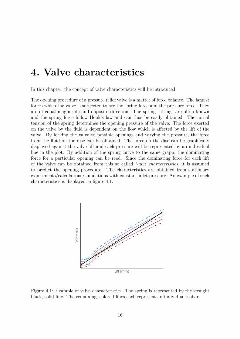
The opening procedure of a pressure relief valve is a matter of force balance. The largestforces which the valve is subjected to are the spring force and the pressure force. Theyare of equal magnitude and opposite direction. The spring settings are often knownand the spring force follow Hook’s law and can thus be easily obtained. The initialtension of the spring determines the opening pressure of the valve. The force exertedon the valve by the fluid is dependent on the flow which is affected by the lift of thevalve. By locking the valve to possible openings and varying the pressure, the forcefrom the fluid on the disc can be obtained. The force on the disc can be graphicallydisplayed against the valve lift and each pressure will be represented by an individualline in the plot. By addition of the spring curve to the same graph, the dominatingforce for a particular opening can be read. Since the dominating force for each liftof the valve can be obtained from this so called Valve characteristics, it is assumedto predict the opening procedure. The characteristics are obtained from stationaryexperiments/calculations/simulations with constant inlet pressure. An example of suchcharacteristics is displayed in figure 4.1.

Lift (mm)

Fo

rce

(N

)

Figure 4.1: Example of valve characteristics. The spring is represented by the straightblack, solid line. The remaining, colored lines each represent an individual isobar.

16

The valve will remain closed as long as the spring force is larger than the fluid force.This is represented in the characteristics when the spring curve lies above the isobars.As the pressure rises, the fluid force increases and when the fluid force exceeds thespring force, the valve will start to open. For each lift in the valve characteristics, therewill exist an intersection between some isobar and the spring curve resulting in a forceequilibrium on the disc.

By changing the spring settings, that is, the spring constant and the initial springtension, the spring force on the valve is altered. Hence, the force balance is also modified.The initial spring tension determines the pressure at which the valve will start to openand the spring constant is the slope of the spring curve and consequently the rate atwhich the spring force increase with the valve lift. In addition to changing the springconstant and initial spring tension to change the behaviour of the valve, frictionalelements can be added to the valve to create hysteresis between the opening- andclosing curves of the valve. The effect of adding frictional elements can be visualizedon the characteristics by a second spring curve. When the valve opens, it will followthe original spring but when closing, it will follow the new spring. This means thatin order to close, the pressure must fall to an isobar that lies below the second spring.That is, the spring force must overcome both the fluid pressure force and the frictionalforce (added by the frictional elements) for the valve to close. Figure 4.2 displays thesame characteristics as figure 4.1 with the addition of a second, imaginary spring.

Lift (mm)

Fo

rce

(N

)

Figure 4.2: Example of valve characteristics with hysteresis

To illustrate the effect of the spring settings, two different cases will be presented. Thecases presented describe ideal behaviors for theoretical valves and are only used toillustrate how the characteristics could be analyzed and how different spring settingsmight yield different valve behaviors. Throughout this section, it is assumed that thevalve characteristics predict the transient behavior of the valve well.

17

First, the spring constant is set high, resulting in a steep spring curve, see figure 4.3a.The spring curve has a much steeper incline than the isobars, resulting in that thespring curve only intersects a particular isobar once. For this spring, the pressure hasto continuously increase for the valve to open and the valve will open proportional tothe pressure increase. This would be a so called proportionally opening valve. When thepressure in the system decreases, the valve will close in the same manner, proportionalto the pressure decrease. The opening and the closing of the valve will follow the outlinedisplayed in figure 4.3b1.

Lift (mm)

Fo

rce

(N

)

(a) Characteristics with a high spring con-stant.

Pressure

Lift

Hysteresis

(b) Corresponding opening and closing be-haviour.

In the second case, the spring constant is smaller, creating a less steep spring curve.The spring has an incline which is smaller than the incline of the isobars. This type ofspring can intersect the same isobar twice. That is, the valve has two lifts for the samepressure. this yields a so called popping or high-lifting opening behavior of the valve.A schematic illustration of this can be seen in figure 4.4a.

Lift (mm)

Fo

rce

(N

)

(a) Characteristics with a low spring constant.

Pressure

Lift

(b) Corresponding opening and closing be-haviour.

1Hysteresis has been added to the opening- and closing characteristics of the proportional valve inorder to separate the curves and make the figure easier to analyze. If no additional hysteresis is added,the opening- and closing lines will completely overlap.

18

The spring curve intersects the isobars at two positions. When the valve reaches thefirst of those positions, the disc will pop from that lift directly to the lift of the otherposition. This region is called a high-lifting region. For the valve to reseat again, thepressure must decrease low enough to reach an isobar that lies completely below thespring curve. When the reseating isobar is reached, the valve will pop down to itsclosed position as fast as it popped upwards. This yields an opening/closing curve asdisplayed in figure 4.4b.

A more detailed description of how the valve opening characteristics should be inter-preted is given in the example below.

(a) Schematic force-lift diagram, the valveis fully closed.

(b) Schematic lift-pressure diagram, the valveis fully closed.

Figure 4.5: Schematic diagrams of opening behavior.

In figure 4.5a, the valve is fully closed, the disc position is given by the green marker.The pressure force curve represents the force generated by a constant pressure fordifferent disc positions. The spring force represents the force generated by the springfor different lifts. Figure 4.5b displays how the valve is completely closed even thoughthe pressure is increasing, this is due to that the spring force is higher than the pressureforce.

(a) Schematic force-lift diagram, the valvebegins to open.

(b) Schematic lift-pressure diagram, the valvebegins to open.

Figure 4.6: Schematic diagrams of opening behavior continued.

19

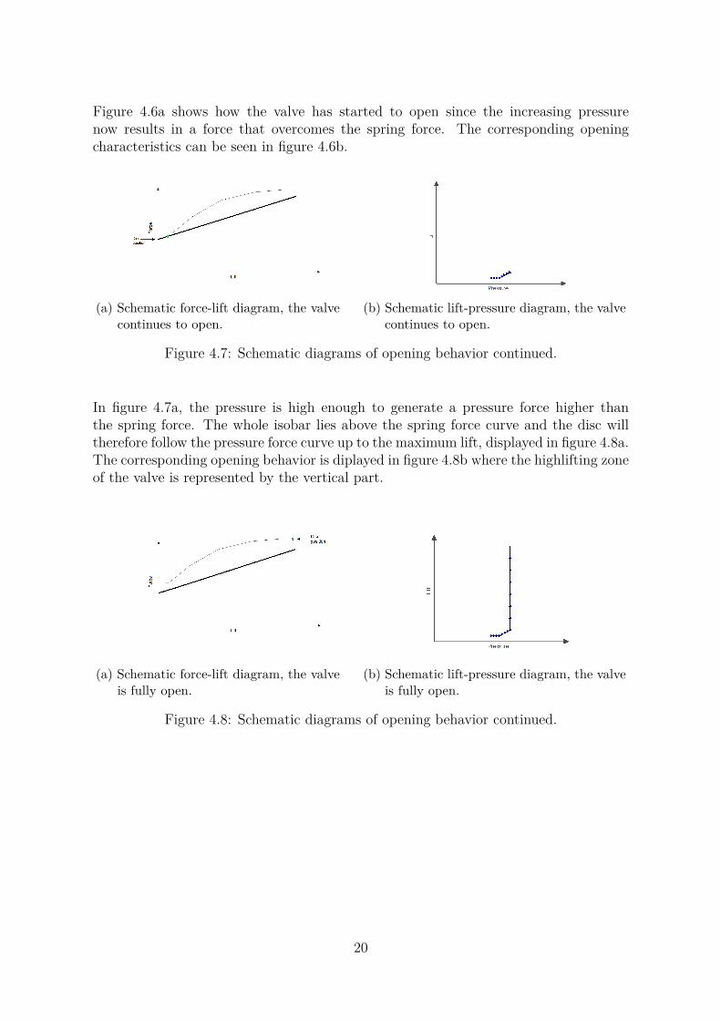
Figure 4.6a shows how the valve has started to open since the increasing pressurenow results in a force that overcomes the spring force. The corresponding openingcharacteristics can be seen in figure 4.6b.

(a) Schematic force-lift diagram, the valvecontinues to open.

(b) Schematic lift-pressure diagram, the valvecontinues to open.


In figure 4.7a, the pressure is high enough to generate a pressure force higher thanthe spring force. The whole isobar lies above the spring force curve and the disc willtherefore follow the pressure force curve up to the maximum lift, displayed in figure 4.8a.The corresponding opening behavior is diplayed in figure 4.8b where the highlifting zoneof the valve is represented by the vertical part.

(a) Schematic force-lift diagram, the valveis fully open.

(b) Schematic lift-pressure diagram, the valveis fully open.


20

5. Hypotheses about valvecharacteristics and stability

In this chapter, some hypotheses regarding the valve characteristics and their applica-tion will be presented first. This will be followed by a section where hypotheses aboutsafety relief valve stability and their operation in different systems will be discussed.

5.1 Valve characteristicsFrom the reasoning presented in the previous section, the spring settings may signifi-cantly change the behavior of the valve. By choosing different values of the spring con-stant, the opening characteristics can be set to, for example, popping or proportional.But is it possible to achieve all these different opening behaviors for any system? Willthe force exerted on the disc by the pressure in the system be the same regardless of theconditions upstreams the pressure relief valve? Presumably, different systems will yielddifferent characteristics and consequently different behaviors. As presented in chapter2, safety valves are often categorized as either popping, proportional or high-lifting, re-gardless of the properties of the system to which the valve is attached. It can be arguedthat a combination of the spring- and the system properties will have to be taken intoaccount prior to the classification of the valve.

Theoretically, the spring can be altered to give a certain opening behavior. By changingthe initial spring tension the opening pressure of the valve can be changed. It should bepossible to create a popping valve for any system, with a spring constant low enough.However, a soft spring will cause the valve to open at a lower pressure than a stiffspring. Additionally, as seen in figure 4.4b, a popping or high-lifting valve experiencehysteresis between the opening and the closing pressure, and in order for the valve toclose, the pressure has to decrease substantially. When aiming for a popping openingbehaviour, the reclosing pressure must be taken into account to ensure that the wholesystem will not be completely dried out before the valve recloses. By having a stiffenough spring, a safety valve can be made more proportional. In contrast to a softerspring, this will yield a higher opening pressure for the valve. It must be made sure thatthe new opening pressure is not higher than the systems design pressure, otherwise, thesystem might be damaged or destroyed prior to the valve opening.

Provided that the valve characteristics can be used to predict the transient response

21

of a safety valve, it represents a fairly easy method of studying safety valves. Thecharacteristics can be generated through steady state simulations which is a muchfaster method than transient simulations and as the examples above have illustrated,the results are easy to analyze. On the basis of these facts, it is therefore of interest tostudy if valve characteristics yields a good enough prediction of the transient responseof a safety valve.

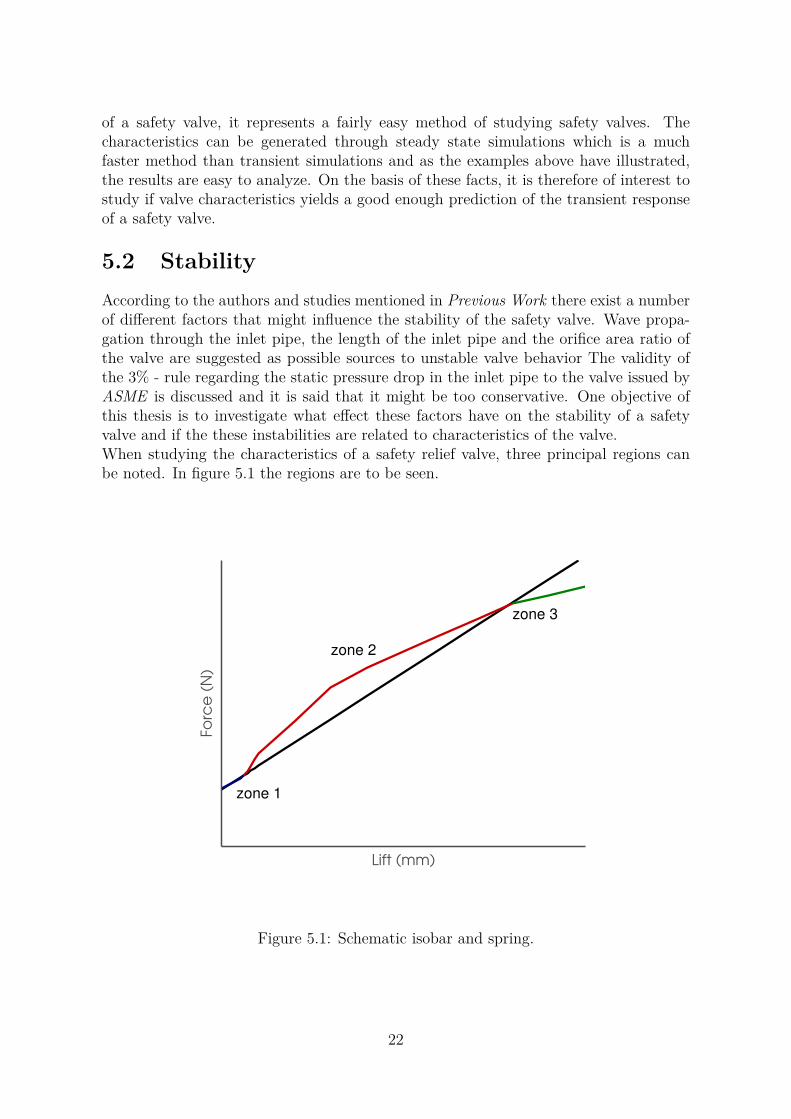
5.2 StabilityAccording to the authors and studies mentioned in Previous Work there exist a numberof different factors that might influence the stability of the safety valve. Wave propa-gation through the inlet pipe, the length of the inlet pipe and the orifice area ratio ofthe valve are suggested as possible sources to unstable valve behavior The validity ofthe 3% - rule regarding the static pressure drop in the inlet pipe to the valve issued byASME is discussed and it is said that it might be too conservative. One objective ofthis thesis is to investigate what effect these factors have on the stability of a safetyvalve and if the these instabilities are related to characteristics of the valve.When studying the characteristics of a safety relief valve, three principal regions canbe noted. In figure 5.1 the regions are to be seen.

Lift (mm)

Fo

rce

(N

)

zone 1

zone 2

zone 3

Figure 5.1: Schematic isobar and spring.

22

• zone 1 - This is an example of an indeterminate region, where the valve can notbe classified as either popping or proportional.

• zone 2 - This is an example of a popping region, where the spring curve liescompletely below the opening isobar, up to the second point of intersection.

• zone 3 - The region after the second point of intersection, resulting from the factthat the isobars deflect due to pressure drop, is proportional. It is claimed to beunstable.

The different zones are associated with different types of problems. It is of interest toexamine if this is valid for all types of system. The possible factors for causing instablebehavior for the zone previously mentioned will be described below.

Zone 1Neither of the forces acting on the valve is dominating and a small perturbation yieldsa large deviation. Classical stability theory proposes that this region would lead toinstabilities. The position of the disc indeterminable by the force balance. Having inmind that the length of the inlet pipe impacts the inertia of the system and the inertiaof the system describes its responsiveness to changes in force and therefore in pressure,it is reasonable to believe that a longer inlet pipe (high inertia) might stabilize the valvebehavior.

Zone 2The popping region, where the valve can be said to have two positions (lifts) for thesame pressure, should result in a rapid decrease of pressure in the system since theopening can be said to be uncontrolled. This is often assumed to be the most unstableregion for incompressible media since it can not withhold the pressure. The pressuredecrease leads to a reclosure, and could also result in chattering. If the pop is rapidenough to cause a pressure change large enough to yield (de)compressive waves, a waterhammer is formed, this is assumed to lead to enhancement of oscillations of the disc.The time of the pressure wave propagation twave, i.e the time it takes for a pressure waveto travel from the valve and be reflected can be expressed as twave = 2L

c. It is suggested

that if twave is shorter than the time it takes for the disc to react to the pressure changebeneath it, the disc will not oscillate and the valve will operate in a stable manner. Fora short enough pipe, the pressure wave might bounce back to the valve before the dischas started to react to the pressure drop created by the opening of the valve. Increasingthe length of the inlet pipe will eventually result in that the pressure wave does notreturn to the valve in time to prevent the disc from closing. But, increasing the lengthof the inlet line also increases the inertia of the system and it is reasonable to believethat eventually, the inertia of the system will be large enough to stabilize the systemand prevent the disc from oscillating even though the pressure wave returns too late.

23

Zone 3The region after the second point of intersection between the isobar and the springis claimed to be unstable and should be avoided by limiting the lift of the valve tothis value. Further, the pressure drop should be limited according to the 3% - rule,a pressure drop exceeding this limit might cause the valve to operate in an unstablemanner. A longer pipe will result in a higher pressure drop and the isobars will deflectmore, the longer the pipe is.

HypothesisThe reasoning above leads to the assumption that there would exist certain lengths ofthe inlet pipe for which the valve would operate stable. If it is not possible to changethe length of the inlet pipe to the valve, and it operates in an unstable way, otherways of stabilizing thee disc must be examined. A pressure wave traveling through thesystem creates fluctuating forces on the disc, disturbing the force balance and makingit oscillate. The oscillations of the disc creates more instabilities in the system whichin turn makes the valve even more unstable. It seems reasonable that by making itharder for the valve to close, the whole system might be stabilized. The same reasoningwould be valid for the opening of the valve but since a safety valve is designed andimplemented in a system in order to relieve the pressure should it become to high, theidea of keeping it from opening seems to counteract its purpose of it. Also, keepingthe valve from closing should increase the capacity of the valve compared to when it isoscillating. Mounting frictional elements on the valve spindle should shift the closingof the valve, requiring the spring force not only to exceed the fluid forces acting on thedisc, but also the extra force that is generated from the frictional elements. Frictionalelements are therefore likely to act stabilizing on the valve behavior.

For the second system 2.4b, the pressure increase at the valve is due to the mass flowthrough the control valve as explained in chapter 2. As long as the mass flow into thesystem is larger than the mass flow through the valve, the pressure in the system willincrease. If the valve has a high-lifting behavior zone 2, there exist a point where themass flow out exceeds the inflow through the control valve. When that point is reached,the volume of media between the control valve and the safety valve will be transportedout of the system. When this happens, the pressure in the system deceases, causingthe valve to close. Once the valve is closed, the inflow to the system is again, largerthan the outflow and the pressure starts to build up again. Since the pressure reliefonly occurs when the outflow through the safety valve is larger than the inflow throughthe control valve, a larger inflow of mass requires a higher lift in order of the pressureto be relieved. Regardless of the magnitude of the mass flow, the previous reasoningregarding the existence of a point at which the valve would reclose due to a sufficientlylarge outflow is assumed to be valid. Thus, for a large inflow, that point is shifted toa higher lift which means that the oscillations of the disc will have a larger amplitudethan for a small inflow of mass. When the inflow to the system is high enough, thevalve must reach its maximum lift in order to relieve the system and the disc will thenbecome stable again. From this reasoning, it can be suggested that there exist certainmass flow for which the valve will behave stable. Correspondingly, there will exist aninterval of mass flows that result in an unstable behavior of the valve.

24

If this suggestion proves valid, it is possible to predict an unstable behavior by studyingthe mass flows that the valve is likely to be submitted to. In figure 5.2 a schematicvalve characteristic with examples of schematic iso-lines for mass flows are displayed.The force acting on the disc will be dependent on the mass flow in to the valve. Theshape of the iso-lines for the mass flow are exponential.

Lift (mm)

Fo

rce

(N

)

m1

m2

Figure 5.2: Valve characteristics with schematic mass flow iso-lines.

A valve with characteristics as displayed in figure 5.2 would, based on the presviousreasoning, exhibit a stable operation for mass flows less than m1 kg/s and larger thanm2 kg/s. For mass flows between m1 kg/s and m2 kg/s, an unstable behavior could beexpected.

25

It seems reasonable to believe that the pressure relief process will be faster if the volumeof fluid between the control valve and the safety valve is small. This means that fora small volume, potential oscillations are likely to have a high frequency compared toif the volume is large. A small volume is therefore more prone to yield damaging,high-frequency oscillations. The magnitude of the fluid volume between the controlvalve and the safety valve is thought to be of different importance for liquid- and vaporsystems. Liquid media is more incompressible than a gaseous one and cannot fill thevoid produced by the valve opening as well as a gaseous media. In order to stabilizea liquid system, the volume must therefore be larger than for a vapor. Presumably, avalve with a behavior of the type that can be found in zone 2 would behave differently ifsubjected to a to a source of constant mass inflow or a source of constant pressure. Thisis important to consider since as described in 2.5 valves are often tested for upstreamconditions of the first type but are more likely to be subjected to upstream conditionsof the second type in real pressure protection scenarios.

The hypotheses presented in this section will be investigated through numerical simu-lations of a safety valve.

26

6. Numerical model

In this thesis, the stability of a safety valve will be studied using Computational FluidDynamics (CFD). This chapter will present the mesh and geometry used and the sim-ulations that have been executed to examine the behavior of the valve. First, a briefexplanation of the governing equations that are solved in CFD - simulations will begiven.

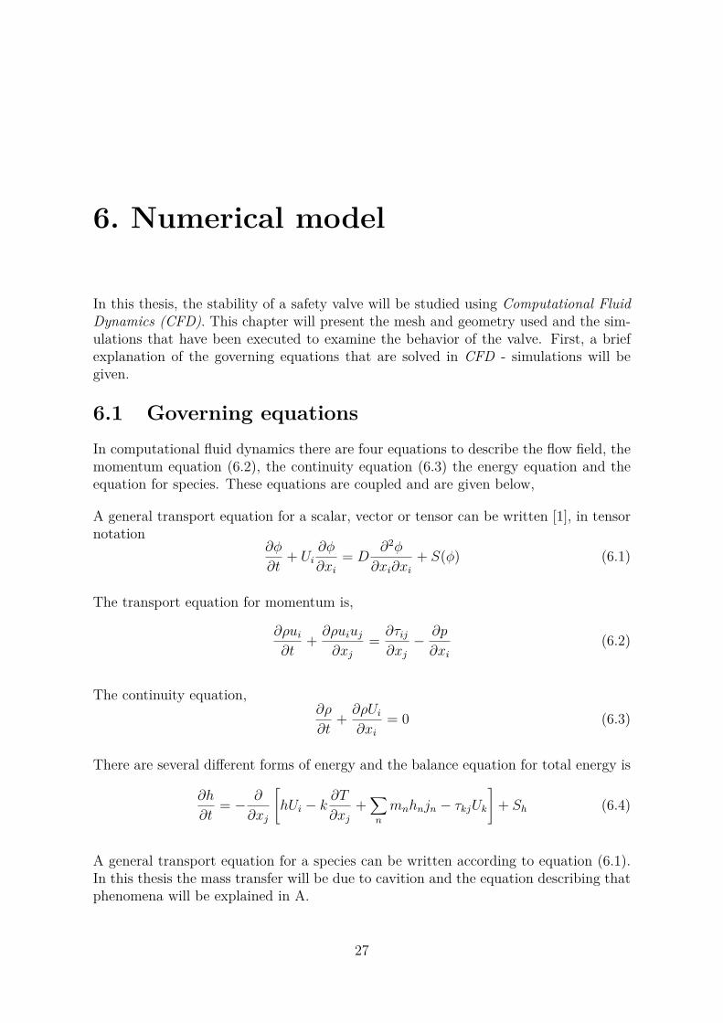
6.1 Governing equationsIn computational fluid dynamics there are four equations to describe the flow field, themomentum equation (6.2), the continuity equation (6.3) the energy equation and theequation for species. These equations are coupled and are given below,

A general transport equation for a scalar, vector or tensor can be written [1], in tensornotation

∂φ

∂t+ Ui

∂φ

∂xi= D

∂2φ

∂xi∂xi+ S(φ) (6.1)

The transport equation for momentum is,

∂ρui∂t

+ ∂ρuiuj∂xj

= ∂τij∂xj− ∂p

∂xi(6.2)

The continuity equation,∂ρ

∂t+ ∂ρUi

∂xi= 0 (6.3)

There are several different forms of energy and the balance equation for total energy is

∂h

∂t= − ∂

∂xj

[hUi − k

∂T

∂xj+∑n

mnhnjn − τkjUk]

+ Sh (6.4)

A general transport equation for a species can be written according to equation (6.1).In this thesis the mass transfer will be due to cavition and the equation describing thatphenomena will be explained in A.

27

In addition to solving the momentum equation and the continuity equation, equationsdescribing the turbulence are to be solved. The turbulence model mainly used in thisthesis is the SST k − ω- Shear stress transport. It is a so called two-equation model,with two additional transport equations for turbulent kinetic energy, k and specificdissipation, ω. The equations are derived from Reynolds average decomposed Navierstokes equation and is based on the Boussinesque approximation, that the Reynoldstresses arising from averaging can be modeled with a turbulent viscosity.

In the regions near the walls, the flow is laminar and the Reynolds number is low, thisregion can not be well represented by equations describing the turbulent flow far fromthe walls. The SST − k − ω model handles the transition between the laminar flow inthe viscous subregion and the fully turbulent flow with a blending function.

The transport equation for turbulent kinetic energy in the k − ω − SST model is,

∂

∂t(ρk) + ∂

∂xi(ρkui) = ∂

∂xj

(Γk

∂k

∂xj

)+ Gk − Yk + Sk (6.5)

• Gk - generation of turblent kinetic energy from mean velocity gradients

• Yk - dissipation of turbulent kinetic energy

• Γk - Effective diffusivity of turbulent kinetic energy

• Sk - source term

The transport equation for the specific dissipation ω is,

∂

∂t(ρω) + ∂

∂xj(ρωuj) = ∂

∂xj

(Γω

∂ω

∂xj

)+Gω − Yω +Dω + Sω (6.6)

• Gω - generation of specific dissipation.

• Yω - dissipation of specific dissipation.

• Γω - Effective diffusivity of specific dissipation.

• Sω - source term for specific dissipation.

28

6.2 Mesh and geometryFor the simulations in this thesis, a 2D - axisymmetric model have been used. Thegeometry was created in Ansys Design Modeler.

a

b

c

d

e

f

g

h

Figure 6.1: The geometry

The most important dimensions for visualizing the valve are presented in table 6.1.

Table 6.1: Dimensions of the geometry

Notation Dimension (mm)a 125b 159.64c 54.1d 60.5e 51.8f 55g 78h 115.01

Dimensions a, b and g were varied to create inlet pipes of different length and diameter.

29

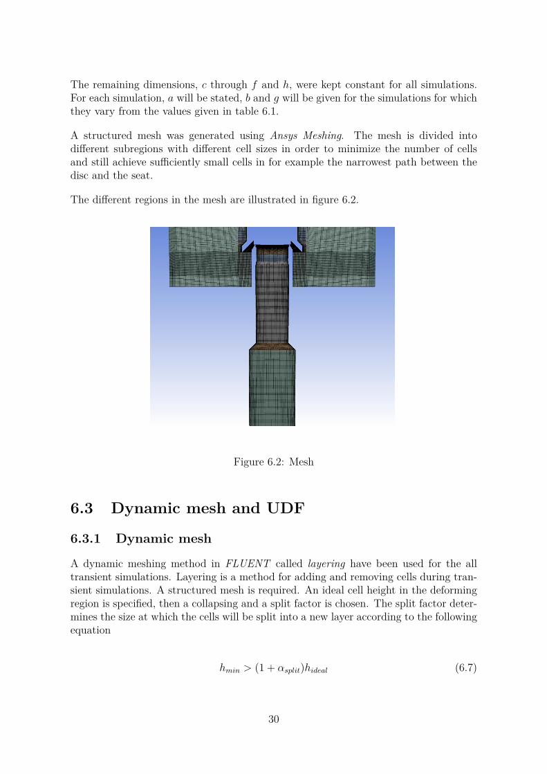
The remaining dimensions, c through f and h, were kept constant for all simulations.For each simulation, a will be stated, b and g will be given for the simulations for whichthey vary from the values given in table 6.1.

A structured mesh was generated using Ansys Meshing. The mesh is divided intodifferent subregions with different cell sizes in order to minimize the number of cellsand still achieve sufficiently small cells in for example the narrowest path between thedisc and the seat.

The different regions in the mesh are illustrated in figure 6.2.

Figure 6.2: Mesh

6.3 Dynamic mesh and UDF

6.3.1 Dynamic mesh

A dynamic meshing method in FLUENT called layering have been used for the alltransient simulations. Layering is a method for adding and removing cells during tran-sient simulations. A structured mesh is required. An ideal cell height in the deformingregion is specified, then a collapsing and a split factor is chosen. The split factor deter-mines the size at which the cells will be split into a new layer according to the followingequation

hmin > (1 + αsplit)hideal (6.7)

30

The collapsing factor, on the otter hand, determines the height at which the cells willmerge together to remove a cell layer.

hmin < αcollapshideal (6.8)

The splitting and merging of cells can also be performed based on cell height ratiosinstead of cell heights [6].

6.3.2 UDF

The UDF contains routines for saving data, moving the disc and controlling the inletpressure. The force in each cell adjacent to the disc is calculated by multiplying thepressure in each cell with the surface area of that cell on the disc boundary. The totalforce on the disc is the achieved by adding all these forces together. The spring forceis calculated using the spring constant and the initial spring tension as described insection 3. The sum of the spring force and the total force is the net force acting on thedisc which determines its direction of movement.

To make the movement of the disc more stable, that is to prevent it from flutteringand to achieve a reseating pressure that is lower than the opening pressure, hysteresiscan be added to the valve. When the velocity of the valve is negative, that is whenthe valve is attempting to close, the difference between the spring force and the totalpressure force must exceed the value of the hysteresis constant specified by the user.

6.4 SimulationsThis section will describe the different simulations that have been made during thisthesis. For the transient simulations, some additional methods needed in FLUENTwill also be presented. Detailed settings used for the simulations can be found inappendix C. The simulations will be divided into two parts corresponding to the twocases presented in section 5.2

In transient simulations, the disc is not fixed to different lifts. The movement of the discis determined by the forces described in section 3 and carried out through a User DefinedFunction (UDF). To preserve the mesh quality from the steady state simulations, themesh must be deformable during the transient simulations. A brief explanation of thedynamic mesh method and the UDF will be given later in this section. Last in thissection, the method for attaining the formula for the pressure drop used in the discretepressure drop - simulations will be explained.

31

6.4.1 Constant pressure

The objective of these simulations is to investigate the usefulness of valve characteristicsto predict the transient response of the safety valve and study the effects of frictionalhysteresis, length of inlet pipe and pressure drop. A pressure-inlet boundary conditionhas been applied to all simulations of case 1.

6.4.1.1 Steady state

• 0.125m (a = 0.125m) inlet pipe

• 20m (a = 20m) inlet pipe

6.4.1.2 Transient

• Inlet line of 0.125m and 20m to compare with the steady state valve character-istics.

• Inlet line of 2m (a = 2m) with and without frictional hysteresis.

• Inlet line of 2m without hysteresis and with modified spring settings. The springconstant was increased and decreased by 30%

• Inlet lines of 0.125m, 0.5m (a = 0.5m) , 2m, 5m (a = 5m), 10m (a = 10m),15m (a = 15m) and 20m without frictional hysteresis to study the impact of thepipe lenght.

• Inlet lines of 0.125m, 0.5m , 2m, 5m, 10m, 15m and 20m with frictional hys-teresis to study the impact of the systems inertia.

• Inlet line of 0.025m (a = 0.025m) and a discrete pressure drop identical to thereal pressure drop for an inlet line of 20m

• Inlet line of 0.025m (a = 0.025m) and a discrete pressure drop of 10%, 25% and50%.

For all transient simulations of case 1, the pressure ramp has followed equation (6.9).

P = 33 + 1.875t bar(g) (6.9)

32

6.4.2 Constant mass flow

The simulations for this case aim at investigating the effect of different mass flowsthrough the system and of the magnitude of the volume between the control valve andthe safety valve. For these simulations, a velocity-inlet boundary condition has beenapplied at the system inlet.

6.4.2.1 Transient

• Inlet line of 5m (a = 5m) and a diameter of 0.1m (g = 0.1m), case I.

• Inlet line of 5m (a = 5m) and a diameter of 0.4m (g = 0.4m), case II.

• Inlet line of 5m (a = 5m) and a diameter of 0.4m (g = 2m), case III.

• Inlet line of 5m (a = 5m), diameter of 0.4m (g = 0.4m) and intermediate pipelength of 20m (b = 20m), case IV.

The velocity ramp for the simulations of case 2 was determined in such a way that themass flow through the valve was equal in time. Equation (6.10) defines the expressionused and the values for each simulation case are defined in table 6.2.

v = vstart + vinctm/s (6.10)

Table 6.2: Velocity ramp factors.

Case vstart (m/s) vinc (m/s)I 0.666 10.000II 0.041 0.608III 0.002 0.025IV 0.034 0.608

6.4.2.2 Pressure drop

Steady state simulations with a 20m long inlet pipe were peformed in order to measurethe pressure 0.15054m from the disc (a = 0.025m). Knowing the inlet pressure, thepressure drop can then be determined. Two different inlet pressures 31 bar(g) and32 bar(g), each with discrete lifts ranging from 0mm to 10mm where simulated.It is assumed that the head loss in the pipe can be predicted by equation (6.11), whichshows how the loss due to friction is dependent on the average velocity of the fluid flow.

P1 − P2 = Cvα (6.11)

P1 refers to the inlet pressure, P2 to the pressure further downstreams (at 0.275m fromthe disc) and v is the average velocity.

33

The coefficients C and α can be found by making a polynomial fitting of the data.The pressure loss in the 20m long pipe can then be represented and replicated with ageometry where the inlet is located 0.15054m from the disc. This is done by applyingequation 6.11 to the inlet pressure in this new geometry. P1 is the pressure used in thesimulations with the longer pipe and the inlet pressure for the shorter pipe will be P2.

The graphical representation of the polynomial fitting of the pressure loss equation canbe seen in figure (6.3).

0 2 4 6 8 10 12 14 16 18 20

0

0.5

1

1.5

2

2.5

3

3.5x 10

5

Velocity (m/s)

Pre

ssu

re d

rop

(P

a)

Figure 6.3: Graphical representation of the polynomial fitting of the pressure loss [Pa]in the 20m long pipe for different lifts [mm].

For the curve presented in figure 6.3, C = 1785.4 and α = 1.8163 which is close to thetheoretical value α = 2, that can be expected for pipe flow. These values have been usedto replicate the pressure drop for the 20m - pipe. For the simulations investigating theeffect of pressure drops of 10%, 25% and 50% magnitude, the constant C in equation(6.3) was varied while α was set constant. To calculate values of C, the followingequation was used.

C = X · 1.1Popenvα

(6.12)

X was set to 0.1, 0.25 and 0.5 to produce a C for each pressure drop.

34

6.5 Sensitivity analysis

6.5.1 Mesh independence

In order to investigate if the solutions were mesh independent, the base mesh wasrefined in the regions closest to the disc. The refined mesh consisted of 45000 cellscompared to the original mesh with 33000 cells at an initial lift of 0.5mm. Steady statesimulations were run for four different lifts, 0.5mm,4mm, 6mm and 8mm and twodifferent pressures, 31 bar(g) and 32 bar(g), and the fluid force on the disc was studied.

The mesh-test simulations showed that the force on the disc was very similar for theoriginal mesh and the refined mesh. The maximum deviation was seen at a lift of 8mmand a pressure of 32 bar(g) where the refined mesh generated a force 0.75% larger thanthe original mesh.The difference in force between the original and the refined mesh wassmall enough to be negligible, that is, the original mesh yielded a mesh independentsolution.

6.5.2 Turbulence model

To validate the choice of turbulence model, steady state simulations with k-ε- modeland non-equilibrium wall function/enhanced wall function were carried out for twopressures, 31 bar(g) and 32 bar(g) and lifts 0.5mm,6mm and 8mm and the resultingforce on the disc was compared to the force generated whit SST/k-ω.

The results show that the k-ε-model predicted a higher force than SST/k-ω for all casesexcept for 8mm lift. The maximum deviation was reached for a lift of 4mm where k-εpredicted/yielded a disc force 0.4% larger than SST/k-ω. At 8mm, SST/k-ω predicteda force 0.5% higher than k-ε.

The deviation between the two turbulence models was very small and therefore, either ofthem would be an appropriate choice. However, the SST-kω proved to yield convergedsolutions more easily and was therefore chosen for all simulations throughout this thesis.

It is important to have in mind that the geometry upstreams the valve is rather simpleand the flow will mainly be along the axial direction of the pipe. A different pipeconfiguration, with for example a bend would result in a different flow pattern withmore vorticity. Not completely resolving the time dependent turbulence would thenlead to a misprediction of the fluid force acting on the disc. However, with the prevailinggeometry, it is most likely the mechanical energy forms, such as the pressure, whichdetermines the amount of energy in the fluid as it interacts with the disc.

35

6.5.3 Courant number and time-step

The Courant number (CFL) is an important parameter in transient CFD simulations.It relates the chosen time step to the time it takes for the flow to pass through a celland is defined as in equation (6.13).

CFL = u∆t∆x (6.13)

u is the velocity for propagation of information (for example velocity of the flow velocityof pressure propagation), ∆t is the time step and ∆x is the length of a cell in thedirection of the flow. CFL > 1 means that the time it takes for the flow to passthrough a cell is smaller than the time step at which the solver advances (for an explicitsolver). This means that some cells might be entirely skipped by the solver and theresulting values will therefore deviate from the true ones. By changing the cell size orthe time step, the CFL - number can be changed to meet the requirements of the solver.

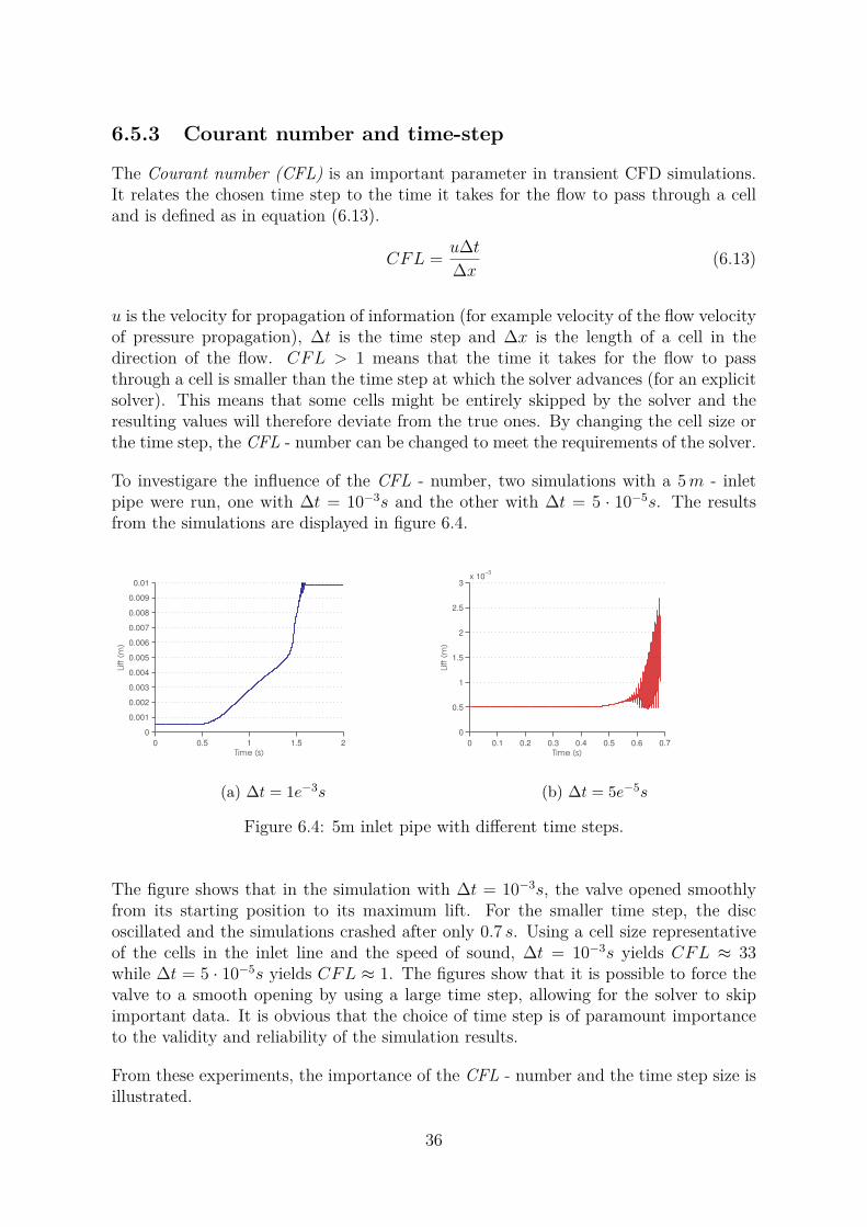
To investigare the influence of the CFL - number, two simulations with a 5m - inletpipe were run, one with ∆t = 10−3s and the other with ∆t = 5 · 10−5s. The resultsfrom the simulations are displayed in figure 6.4.

0 0.5 1 1.5 2

0

0.001

0.002

0.003

0.004

0.005

0.006

0.007

0.008

0.009

0.01

Time (s)

Lift

(m)

(a) ∆t = 1e−3s

0 0.1 0.2 0.3 0.4 0.5 0.6 0.7

0

0.5

1

1.5

2

2.5

3x 10

−3

Time (s)

Lift

(m)

(b) ∆t = 5e−5s

Figure 6.4: 5m inlet pipe with different time steps.

The figure shows that in the simulation with ∆t = 10−3s, the valve opened smoothlyfrom its starting position to its maximum lift. For the smaller time step, the discoscillated and the simulations crashed after only 0.7 s. Using a cell size representativeof the cells in the inlet line and the speed of sound, ∆t = 10−3s yields CFL ≈ 33while ∆t = 5 · 10−5s yields CFL ≈ 1. The figures show that it is possible to force thevalve to a smooth opening by using a large time step, allowing for the solver to skipimportant data. It is obvious that the choice of time step is of paramount importanceto the validity and reliability of the simulation results.

From these experiments, the importance of the CFL - number and the time step size isillustrated.

36

The Courant number presented above are calculated using a cell size representativeof the pipe. However, the cells closest to the disc are significantly smaller, yielding amuch higher CFL. This results in that the velocity at which pressure wave propagatesin the system is overestimated. The time step used in the simulations is not sufficientto resolve the pressure wave propagation.

6.5.4 Compressibility

Liquids are often considered incompressible with a constant density. Modeling a liquidas incompressible results in an infinite speed of sound in the liquid, according to equation(6.14),

c =√

1χρ

(6.14)

where χ is the compressibility factor defined as χ = 1ρ∂ρ∂P

.

If an acoustic wave propagates through the safety relief valve system infinitely fast, thedisc will not have time to react to the pressure decrease below it, since the pressure isrestored infinitely fast. By comparing the opening behavior for the valve, attached toan inlet line of 2m without hysteresis, where the fluid is modeled as compressible andincompressible, it can be seen that with the simplification of incompressibility a lot ofinformation is lost, see figure 6.5. It is noted that the valve behaves completely stablewhen the fluid is modeled as incompressible, which is not the case when the liquid isconsidered compressible and the valve chatters.

0 0.2 0.4 0.6 0.8 1 1.2 1.4

0

0.001

0.002

0.003

0.004

0.005

0.006

0.007

0.008

0.009

0.01

Time (s)

Lift

(m)

(a) Incompressible

0.4 0.45 0.5 0.55

0

1

2

3x 10

−3

Time (s)

Lift

(m)

(b) Compressible

Figure 6.5: Opening behavior of safety relief valve attached to an inlet line of 2m.Comparison of compressible and incompressible fluid.

37

7. Numerical results

In this chapter, the results from the numerical simulations will be presented. Theresults will be divided in accordance with the two cases presented in section 2.5 andthe different effects corresponding to each case.

7.1 Constant pressureIn this section the results from the simulations with constant pressure boundary con-dition will be presented.

7.1.1 Characteristics and opening behavior

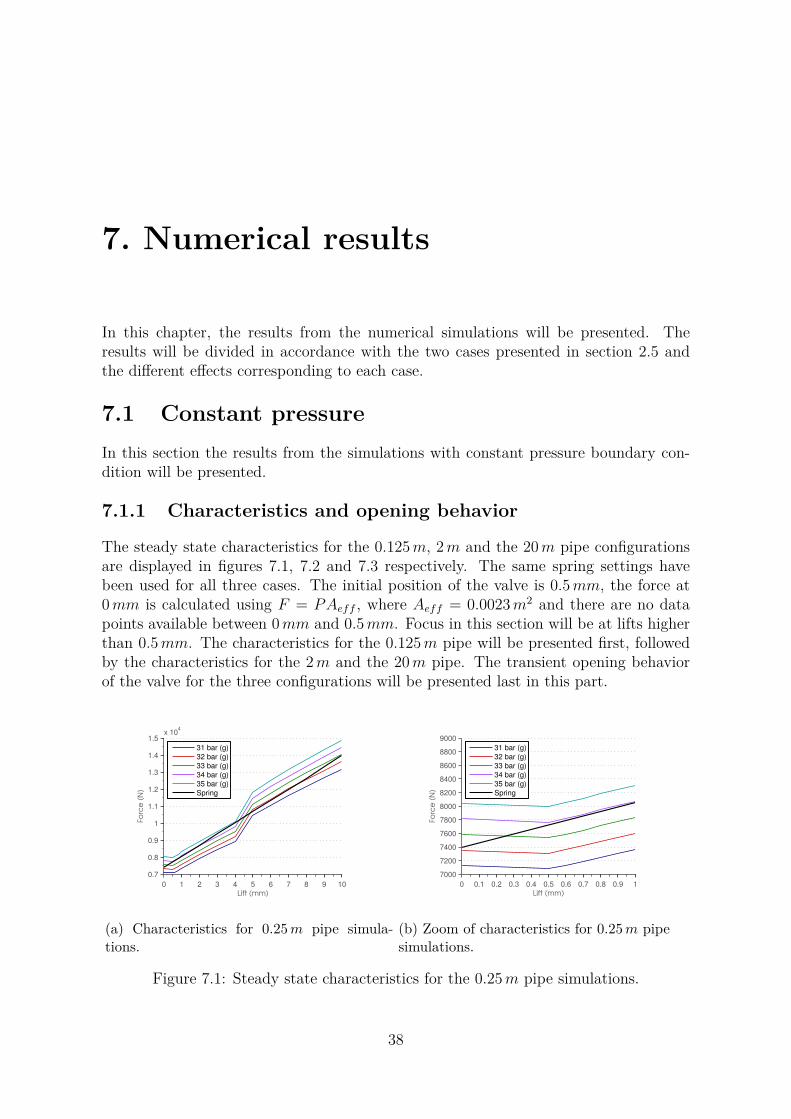
The steady state characteristics for the 0.125m, 2m and the 20m pipe configurationsare displayed in figures 7.1, 7.2 and 7.3 respectively. The same spring settings havebeen used for all three cases. The initial position of the valve is 0.5mm, the force at0mm is calculated using F = PAeff , where Aeff = 0.0023m2 and there are no datapoints available between 0mm and 0.5mm. Focus in this section will be at lifts higherthan 0.5mm. The characteristics for the 0.125m pipe will be presented first, followedby the characteristics for the 2m and the 20m pipe. The transient opening behaviorof the valve for the three configurations will be presented last in this part.

0 1 2 3 4 5 6 7 8 9 10

0.7

0.8

0.9

1

1.1

1.2

1.3

1.4

1.5x 10

4

Lift (mm)

Fo

rce

(N

)

31 bar (g)

32 bar (g)

33 bar (g)

34 bar (g)

35 bar (g)

Spring

(a) Characteristics for 0.25 m pipe simula-tions.

0 0.1 0.2 0.3 0.4 0.5 0.6 0.7 0.8 0.9 1

7000

7200

7400

7600

7800

8000

8200

8400

8600

8800

9000

Lift (mm)

Fo

rce

(N

)

31 bar (g)

32 bar (g)

33 bar (g)

34 bar (g)

35 bar (g)

Spring

(b) Zoom of characteristics for 0.25 m pipesimulations.

Figure 7.1: Steady state characteristics for the 0.25m pipe simulations.

38

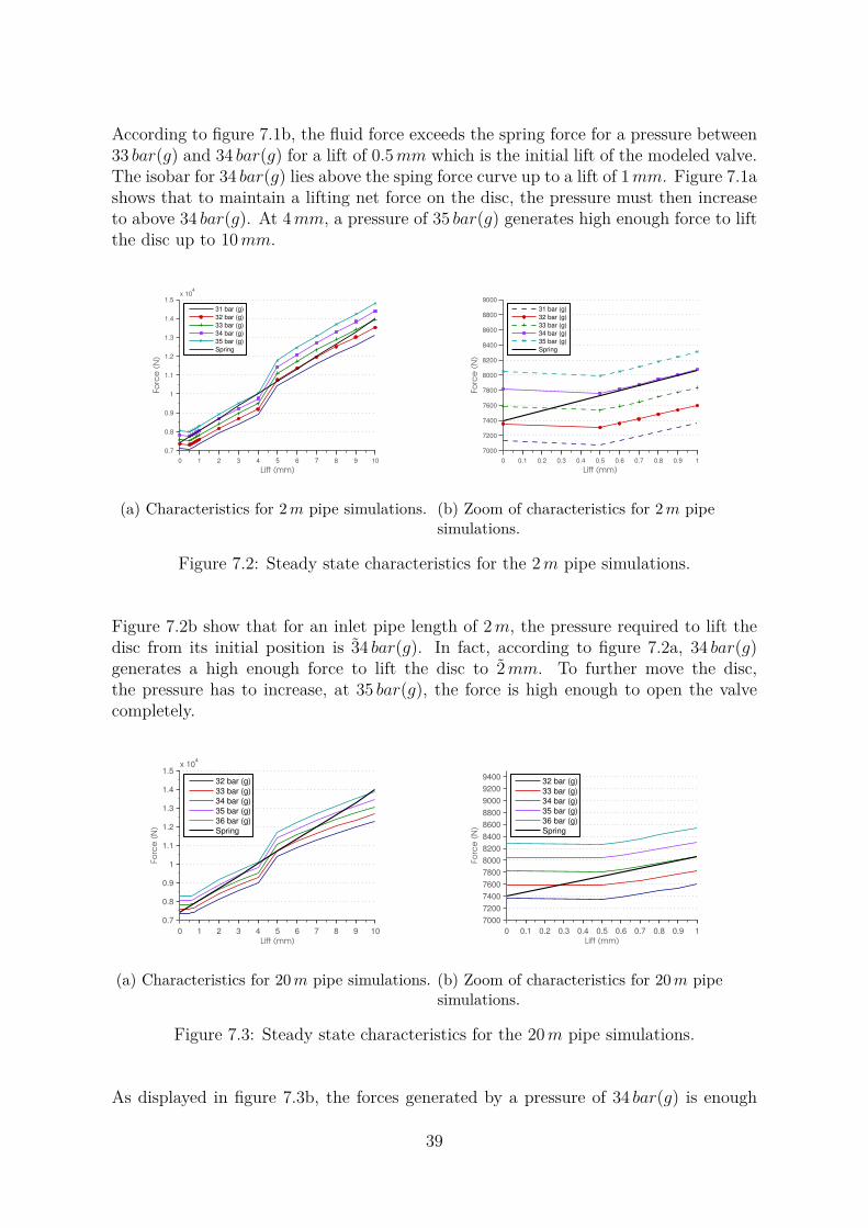
According to figure 7.1b, the fluid force exceeds the spring force for a pressure between33 bar(g) and 34 bar(g) for a lift of 0.5mm which is the initial lift of the modeled valve.The isobar for 34 bar(g) lies above the sping force curve up to a lift of 1mm. Figure 7.1ashows that to maintain a lifting net force on the disc, the pressure must then increaseto above 34 bar(g). At 4mm, a pressure of 35 bar(g) generates high enough force to liftthe disc up to 10mm.

0 1 2 3 4 5 6 7 8 9 10

0.7

0.8

0.9

1

1.1

1.2

1.3

1.4

1.5x 10

4

Lift (mm)

Fo

rce

(N

)

31 bar (g)

32 bar (g)

33 bar (g)

34 bar (g)

35 bar (g)

Spring

(a) Characteristics for 2 m pipe simulations.

0 0.1 0.2 0.3 0.4 0.5 0.6 0.7 0.8 0.9 1

7000

7200

7400

7600

7800

8000

8200

8400

8600

8800

9000

Lift (mm)Fo

rce

(N

)

31 bar (g)

32 bar (g)

33 bar (g)

34 bar (g)

35 bar (g)

Spring

(b) Zoom of characteristics for 2 m pipesimulations.

Figure 7.2: Steady state characteristics for the 2m pipe simulations.

Figure 7.2b show that for an inlet pipe length of 2m, the pressure required to lift thedisc from its initial position is 34 bar(g). In fact, according to figure 7.2a, 34 bar(g)generates a high enough force to lift the disc to 2mm. To further move the disc,the pressure has to increase, at 35 bar(g), the force is high enough to open the valvecompletely.

0 1 2 3 4 5 6 7 8 9 10

0.7

0.8

0.9

1

1.1

1.2

1.3

1.4

1.5x 10

4

Lift (mm)

Fo

rce

(N

)

32 bar (g)

33 bar (g)

34 bar (g)

35 bar (g)

36 bar (g)

Spring

(a) Characteristics for 20 m pipe simulations.

0 0.1 0.2 0.3 0.4 0.5 0.6 0.7 0.8 0.9 1

7000

7200

7400

7600

7800

8000

8200

8400

8600

8800

9000

9200

9400

Lift (mm)

Fo

rce

(N

)

32 bar (g)

33 bar (g)

34 bar (g)

35 bar (g)

36 bar (g)

Spring

(b) Zoom of characteristics for 20 m pipesimulations.

Figure 7.3: Steady state characteristics for the 20m pipe simulations.

As displayed in figure 7.3b, the forces generated by a pressure of 34 bar(g) is enough

39

to lift the disc from its initial position of 0.5mm. In order to reach a lift higher than1mm the pressure in the system has to increase, this can be observed in figure 7.3a.For a constant pressure of 35 bar(g), the forces are high enough to reach a lift of 3mm.A pressure of 36 bar(g) lifts the disc to 10mm.

From figures 7.1 and 7.3 it can be noted that the maximum force for the 20m pipe aresignificantly lower than for the 0.125m pipe. It can also be noted that for lifts between0.5mm and 2mm, the spring force curve tangents the isobar of 34 bar(g) for all threeconfigurations.

The transient respons for the 0.125m and 20m configurations will now be presented.The transient respons for the system with an inlet line of 2m proved to be very unstableand will be presented later in this chapter.

3.3 3.4 3.5

x 106

0

0.001

0.002

0.003

0.004

0.005

0.006

0.007

0.008

0.009

0.01

Pressure (Pa)

Lift

(m)

(a) Zoom of characteristics for 0.125 m pipesimulations.

3.3 3.4 3.5 3.6 3.7 3.8

x 106

0

0.001

0.002

0.003

0.004

0.005

0.006

0.007

0.008

0.009

0.01

Pressure (Pa)

Lift

(m)

(b) Transient respons for 20 m pipe simula-tions.

Figure 7.4: Transient respons for 20m - pipe and 0.125m-pipe simulations.

The transient response of the valve connected to an inlet pipe of 0.125m is displayedin figure 7.4a. The opening starts at a pressure just below 34 bar(g) and the discreaches 2.5mm at a pressure of 34 bar(g). Between 34 and 35 bar(g), the valve opensproportionally to the pressure increase. At 35 bar(g) and 4mm, the disc high-lifts to10mm where it stabilizes. Figure 7.4b shows the transient opening behavior for thesystem with a 20m - inlet pipe. The valve starts to open at a pressure of 34 bar(g)and opens proportional to the pressure increase until 37 bar(g) and 5mm is reached.Between 5 and 5.5mm the valve experience a high-lifting zone only to continue itsproportional behavior until the maxmimum lift is reached for a pressure of 38 bar(g).

In figure 7.5, the isobar of 32 bar(g) is graphically displayed for inlet pipe lengths of0.125m and 20m.

40

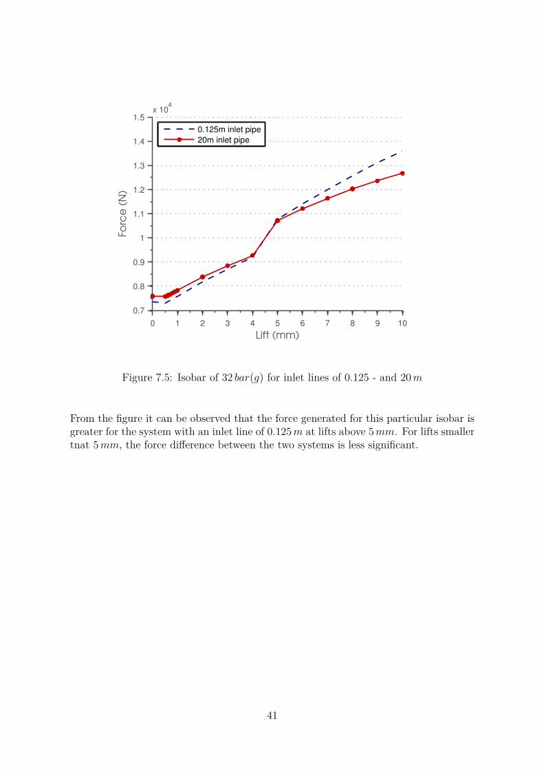
0 1 2 3 4 5 6 7 8 9 10

0.7

0.8

0.9

1

1.1

1.2

1.3

1.4

1.5x 10

4

Lift (mm)

Fo

rce

(N

)

0.125m inlet pipe

20m inlet pipe

Figure 7.5: Isobar of 32 bar(g) for inlet lines of 0.125 - and 20m

From the figure it can be observed that the force generated for this particular isobar isgreater for the system with an inlet line of 0.125m at lifts above 5mm. For lifts smallertnat 5mm, the force difference between the two systems is less significant.

41

7.1.2 Effect of hysteresis

To illustrate the effect of hysteresis, the results from the simulations with a 2m inlet pipewill be presented. Figure 7.6 shows the opening behavior of the valve with hysteresis(7.6a) and without hysteresis (7.6b).

0 0.2 0.4 0.6 0.8 1 1.2

0

0.001

0.002

0.003

0.004

0.005

0.006

0.007

0.008

0.009

0.01

Time (s)

Lift

(m)

(a) With hysteresis.

0.4 0.45 0.5 0.55

0

1

2

3x 10

−3

Time (s)

Lift

(m)

(b) Without hysteresis.

Figure 7.6: Transient simulations with a 2m inlet pipe.

When comparing the opening behaviors of the valve with hysteresis (figure 7.6a) and theone without (fig 7.6b), the difference is easily observed. When subjected to hysteresis,the valve opens smoothly from 0.5mm to 10mm, experiencing a more proportionalbehavior between 0.5mm and 5mm and a high lifting part between 5mm and themaximum lift. When the valve is simulated without addition of hysteresis, the discstarts to oscillate as soon as the valve starts to open and never reaches the maximumlift of 10mm.

7.1.3 Acoustic pressure wave propagation

To study the occurence and effect of pressure waves propagating through the system,the results from the simulations with a 2m pipe will be used. In figures 7.7 and 7.8,the static pressure along the pipe for different times are presented. The correspondingtimes are marked in figure 7.9 which show the opening behavior of the valve when nohysteresis was added to the system. In water the speed of sound is 1500 m/s, but pressurein the pipe propagates with a velocity that ranges between 1500− 4300 m/s. The wavefront is somewhat diffusive, it should be mentioned that the numerical scheme usedfor the results presented here, is second order accurate and CFL ≈ 1 in the middle ofthe pipe. The dotted line in figures 7.7a through 7.8b represents the vapor pressure ofwater at 298K which is 0.0317 bar.

42

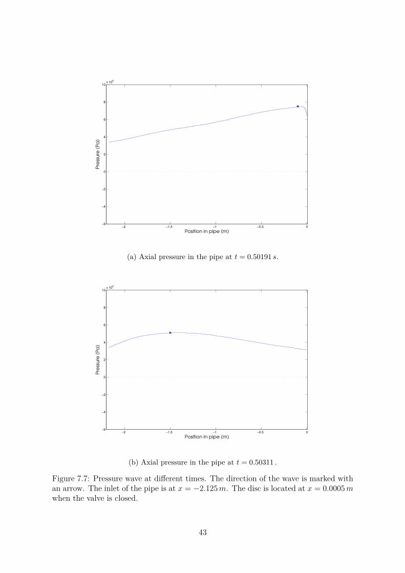
−2 −1.5 −1 −0.5 0−6

−4

−2

0

2

4

6

8

10x 10

6

Position in pipe (m)

Pre

ssu

re (

Pa

)

(a) Axial pressure in the pipe at t = 0.50191 s.

−2 −1.5 −1 −0.5 0−6

−4

−2

0

2

4

6

8

10x 10

6


Pre

ssu

re (

Pa

)

(b) Axial pressure in the pipe at t = 0.50311 .

Figure 7.7: Pressure wave at different times. The direction of the wave is marked withan arrow. The inlet of the pipe is at x = −2.125m. The disc is located at x = 0.0005mwhen the valve is closed.

43

−2 −1.5 −1 −0.5 0−6

−4

−2

0

2

4

6

8

10x 10

6


Pre

ssu

re (

Pa

)

(a) Axial pressure in the pipe at t = 0.50430 s.

−2 −1.5 −1 −0.5 0−6

−4

−2

0

2

4

6

8

10x 10

6


Pre

ssu

re (

Pa

)

(b) Axial pressure in the pipe at t = 0.50630 s.

Figure 7.8: Pressure wave at different times. The direction of the wave is marked withan arrow. The inlet of the pipe is at x = −2.125m. The disc is located at x = 0.0005mwhen the valve is closed.

44

0.45 0.46 0.47 0.48 0.49 0.5 0.51

0

0.5

1

1.5

2

2.5

3x 10

−3

Time (s)

Lift

(m)

Figure 7.9: Lift against time for 2m pipe with different times corresponding to pressurewaves in 7.7 and 7.8.

Comparing the pressure wave positions in figures 7.7a through 7.8b with the openingbehavior in figure 7.9, it can be seen that when the valve has closed, a pressure waveis created at the seat of the valve. At t = 0.50430 s, the valve has opened and pressuresurge is visible in figure 7.8a. The oscillations of the disc thus seem to follow thepressure propagation in the pipe.

7.1.4 Modification of spring

As discussed in chapter 4, different spring settings might yield different opening behav-iors. To evaluate if a valve which chatters can be stabilized by changing the spring,an additional simulation was made with the 2m inlet line. The two additional springtested had the same initial spring tension as the original spring while the spring con-stant was increased or decreased by 30%. The resulting springs are displayed in figure7.10 and the corresponding opening behavior in figure 7.11

45

0 1 2 3 4 5 6 7 8 9 10

0.7

0.8

0.9

1

1.1

1.2

1.3

1.4

1.5x 10

4

Lift (mm)

Fo

rce

(N

)

31 bar (g)

32 bar (g)

33 bar (g)

34 bar (g)

35 bar (g)

Spring1

Spring2

Spring3

Figure 7.10: Valve characteristics for an inlet line of 2m with two modified springs(spring 2 and 3) as well as the original spring (spring 1).

0 0.1 0.2 0.3 0.4 0.5

0

0.001

0.002

0.003

0.004

0.005

0.006

0.007

0.008

0.009

0.01

Time (s)

Lift

(m)

Figure 7.11: Lift versus time for inlet pipe of 2m with spring 2, a spring constantdecreased by 30%

46

Figure 7.11 show that the valve starts to open at t ≈ 0.2 s, which can be compared tot ≈ 0.4 s for the valve with original spring settings presented in figure 7.6. Between1mm and 3mm, the valve experiences a somewhat oscillating region but then stabilizesand continues to open smoothly. The proportional zone observed for the original springsettings is diminished and the opening behavior is slightly more high-lifting. It can benoted that the transient response of the valve is much more stable than that observedfor the original spring settings when no hysteresis was added (figure 7.6b).

7.1.5 Effect of different pipe lengths

To investigate the possible effects of the inertia of the system on the disc behavior, sixsimulations with varying inlet lines lengths were performed. For all these, a frictionalhysteresis of 400N has been applied. The results are displayed in figure 7.12.

0 0.5 1 1.5 2 2.5 3 3.5 4

0

0.001

0.002

0.003

0.004

0.005

0.006

0.007

0.008

0.009

0.01

Time (s)

Lift

(m)

0.5 m

2 m

5 m

10 m

15 m

20 m

Figure 7.12: Lift vs time for different pipe lengths.

As can be seen in this figure, the opening behavior differs for different lengths of theinlet pipe. The high-lifting region that is observed for small lifts for the 0.5m systemtends to take on a more proportional form as the length of the pipe increases. It can alsobe noted that the second high-lifting region, at lifts between 4mm and 10mm for the0.5m pipe, becomes shorter, starts at higher lifts and also becomes less high-lifting forlonger pipes. To furhter illustrate the transition from high-lifting to more proportionalbehavior, the velocity of the disc for the different inlet lines between 5mm and 10mmis calculated. The velocities are displayed in table 7.1.

47

Table 7.1: Velocity of disc for the second high-lifting region.

Length of inlet pipe (m) Velocity (m/s)0.5 0.1172 0.0655 0.03810 0.02315 0.01420 0.009

The values in table 7.1 show that the velocity of the disc for the second high-liftingregion decreases as the inlet pipe becomes longer. Consequently, the behavior seen infigure 7.12 is confirmed.

7.1.6 Effect of pressure drop

Both of the cases displayed in figure 7.15 have been submitted to the same pressuredrop, the 20m pipe through a “natural” pressure drop through the pipe and the 0.025mthrough a discrete pressure drop applied at the inlet.

0 0.5 1 1.5 2 2.5 3

0

0.001

0.002

0.003

0.004

0.005

0.006

0.007

0.008

0.009

0.01

Time (s)

Lift

(m)

20 m

0.1505 m

(a) Lift versus time for a 20 m inlet pipeand a 0.025 m inlet pipe with discretepressure drop.

0 0.5 1 1.5 2 2.5

0

0.001

0.002

0.003

0.004

0.005

0.006

0.007

0.008

0.009

0.01

Time (s))

Lift

(m)

No pressure drop

Discrete pressure drop

(b) Lift versus time for 0.125 m pipe and0.025 m pipe with discrete pressure drop.

Figure 7.13: Lift versus time for pipes with replication of pressure drop in 20m pipe.

For the longer pipe, the valve has a proportional part between 0.5mm and 5mm, ahigh-lifting part between 5mm and 5.5mm and finally a proportional part between5.5mm and its maximum lift. In figure 7.13a it can be seen that when replicatingthe pressure drop in the 20m pipe with a discrete boundary condition, the openingprocedure of the longer pipe is not captured. The main difference between the twocases is that the system with the shorter pipe reacts faster than the system with a

48

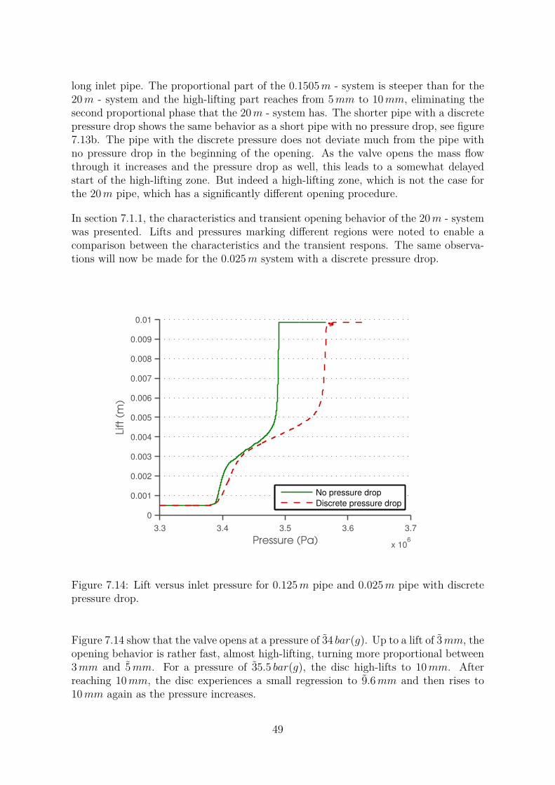
long inlet pipe. The proportional part of the 0.1505m - system is steeper than for the20m - system and the high-lifting part reaches from 5mm to 10mm, eliminating thesecond proportional phase that the 20m - system has. The shorter pipe with a discretepressure drop shows the same behavior as a short pipe with no pressure drop, see figure7.13b. The pipe with the discrete pressure does not deviate much from the pipe withno pressure drop in the beginning of the opening. As the valve opens the mass flowthrough it increases and the pressure drop as well, this leads to a somewhat delayedstart of the high-lifting zone. But indeed a high-lifting zone, which is not the case forthe 20m pipe, which has a significantly different opening procedure.

In section 7.1.1, the characteristics and transient opening behavior of the 20m - systemwas presented. Lifts and pressures marking different regions were noted to enable acomparison between the characteristics and the transient respons. The same observa-tions will now be made for the 0.025m system with a discrete pressure drop.

3.3 3.4 3.5 3.6 3.7

x 106

0

0.001

0.002

0.003

0.004

0.005

0.006

0.007

0.008

0.009

0.01

Pressure (Pa)

Lift

(m)

No pressure drop

Discrete pressure drop

Figure 7.14: Lift versus inlet pressure for 0.125m pipe and 0.025m pipe with discretepressure drop.

Figure 7.14 show that the valve opens at a pressure of 34 bar(g). Up to a lift of 3mm, theopening behavior is rather fast, almost high-lifting, turning more proportional between3mm and 5mm. For a pressure of 35.5 bar(g), the disc high-lifts to 10mm. Afterreaching 10mm, the disc experiences a small regression to 9.6mm and then rises to10mm again as the pressure increases.

49

Further effects of the pressure drop on the valve opening can be seen in figure 7.15.

0 0.5 1 1.5 2 2.5 3 3.5 4

0

0.001

0.002

0.003

0.004

0.005

0.006

0.007

0.008

0.009

0.01

Time (s)

Lift

(m)

No pressure drop

10 % pressure drop

25 % pressure drop

50 % pressure drop

Figure 7.15: Lift versus time for different discrete pressure drops.

It is noted that in all cases the valve starts to open at the same time. However, thelarger the discrete pressure drop is, the more delayed is the high-lifting behavior. It isnot eliminated completely, but the endpoint of the high-lifting zone is at a smaller liftfor larger pressure drops. The discrete pressure drop of 25 % and 50 % seem to have astable point below the maximum lift of the valve where the high-lifting zone ends. Asthe pressure is further increased in time the valve continues to open proportional to theincrease. Non of the discrete pressure drops yield any instabilities.

50

7.2 Constant mass flowIn this section the results from the simulations with the velocity inlet is presented.

7.2.1 Effect of volume

The relationship between the volume of the system and the frequency can be seen intable 7.2. It can be noted that the frequency is decreasing with a larger volume. Thesystems with volumes of 0.628m3 (case II) and 15.708m3 (case III) both stabilizes whenm ≈ 76 kg/s.

Table 7.2: Volume and frequency of oscillatons.

Volume (m3) f(Hz)0.039 175.70.628 24.715.708 3.8

0 0.1 0.2

0

0.001

0.002

0.003

0.004

0.005

0.006

0.007

0.008

0.009

0.01

Time (s)

Lift

(m)

(a) Case I: Volume of 0.039 m3.

0 0.1 0.2 0.3 0.4 0.5 0.6 0.7 0.8 0.9 1

0

0.001

0.002

0.003

0.004

0.005

0.006

0.007

0.008

0.009

0.01

Time (s)

Lift

(m)

(b) Case II: Volume of 0.628 m3.

0 0.1 0.2 0.3 0.4 0.5 0.6 0.7 0.8 0.9 1 1.1

0

0.001

0.002

0.003

0.004

0.005

0.006

0.007

0.008

0.009

0.01

Time (s)

Lift

(m)

(c) Case III: Volume of 15.708 m3.

Figure 7.16: Effect of volume on the transient respons of the valve.

51

7.2.2 Effect of mass flow

As can be seen in figure 7.17 the valve opens rather smoothly and proportionally up to2.5mm. The oscillations are larger the larger the mass flow is, up to m ≈ 50 kg/s wherethe oscillations starts to decay. The valve is completely open and stable for m = 76kg/s.The frequency of the oscillations is constant, only the amplitude is changing.

10 20 30 40 50 60 70 80 90 100 110

0

0.001

0.002

0.003

0.004

0.005

0.006

0.007

0.008

0.009

0.01

Mass flow (kg/s)

Lift

(m

)

Figure 7.17: Opening procedure for case II.

52

7.2.3 Effect of inlet line

In figure 7.19, two geometries with the same volumes are compared, case II and caseIV. It can be seen that for case IV, the oscillations of the system are almost completelyattenuated. Both system reaches their maximum lift for m = 76 kg/s.

(a) Schematic view of geometry with short in-let, case II.

(b) Scematic view of geometry with long inletline, case IV.

Figure 7.18: The two different geometries used.

0 0.1 0.2 0.3 0.4 0.5 0.6 0.7 0.8 0.9 1

0

0.001

0.002

0.003

0.004

0.005

0.006

0.007

0.008

0.009

0.01

Time (s)

Lift

(m)

(a) System with short inlet line, case II.

0 0.1 0.2 0.3 0.4 0.5 0.6 0.7 0.8 0.9 1

0

0.001

0.002

0.003

0.004

0.005

0.006

0.007

0.008

0.009

0.01

Time (s)

Lift

(m)

(b) System with long inlet line, case IV.

Figure 7.19: Effect of pipe length on the transient respons of the valve.

53

8. Analysis and Discussion

The first purpose of this thesis was to investigate if the characteristics of the valvegenerated with steady state simulations can predict the transient response of a safetyrelief valve. When examining the 0.25m pipe it can be concluded that the characteristics(figure 7.1a) predict the transient opening behavior (figure 7.4a) well. The transientbehavior of the 20m pipe deviates from the behavior predicted by the characteristics,see figures 7.3a and 7.4b. The opening pressure is predicted but the high-lifting zonesseen in the steady state predictions are not as distinct in the transient behavior. Theopening of the valve, is not as fast as for the short pipe. The reason for this is thought tobe the inertia of the system, the pressure changes do not instantaneously accelerate thefluid in the pipe, this is a transient effect and will therefore not be captured in the steadystate simulations. In the comparison of the characteristics generated for the long pipe(figure 7.3a), and the replicated discrete pressure drop of the long pipe (figure 7.13a), itcan be noted that the behavior to some extent is predicted. The opening pressure andthe popping zones can be seen in both the characteristics and the transient opening. Thevalve behavior and characteristics are not consistent for intermediate lifts, this regionin the characteristics should be carefully considered since there is a large uncertaintyof the predicted force due to the complicated flow pattern induced by the disc settingsand pressure field. This will be addressed later in this section. Further, the notch seenas the valve is fully opened in the pressure drop replication, is probably due to the factthat the isobars for the longer pipe flattens out and will thus have an additional pointof intersection with the spring.

In the characteristics, figures 7.1a, 7.2a and 7.3a, it can also be seen that for all threelengths presented there is a region where the spring is tangent to some isobar. Asdiscussed in chapter 5, this situations is thought to lead to instabilities where the valveexhibits on-off behavior. As previously stated, the forces are of equal magnitude anda small perturbation of the force equilibrium can therefore result in a large responseof the system. This behavior is confirmed for the 2m pipe which oscillates severely(figure 7.6b).The oscillations follow the pressure propagation in simulation. However,the speed of sound has been observed to take on values significantly higher than whatcan be expected in water. This can be a numerical effect due to the fact that thecomputational cells are too small for the propagation speed of information and the factthat an explicit method have been used to update the time step and the disc positionwhile an implicit method was used for the information propagation. It is important tokeep in mind that the length of the pipe should not be taken as a definite value. As the

54

pressure propagates too fast due to numerics, it will result in the illusion of a shorterpipe.

The 0.125m and the 20m pipe do not show the same oscillating behavior as the 2mpipe, compare figures 7.4 and 7.6b. This is also consistent with what is previouslypresented, that a sufficiently short or long pipe will stabilize the system. In the formerthe pressure source is close to the disc and there is no delay or attenuation of theincreasing force which the increasing inlet pipe length results in. The effect of a longinlet line is confirmed by case II (see section 7.2.1) where two geometries with the samevolume have been studied, one with a short inlet line and the other with a 20m inletline. Studying figure 7.19, it is seen that the system with a 20m - pipe does not oscillatein the same manor as the one with a shorter pipe. The total mass of the systems is thesame in both cases, but the mass that is accelerated is in the inlet pipe, a longer pipewill thus result in more inertia, which will stabilize the system.

To fairly compare the valve characteristics and the transient opening of the valve, thecharacteristics must be generated with the same type of inlet line as the valve is thoughtto be placed on. The valve itself can not be said to behave in a certain way. The behavioris strongly dependent on the system as a whole. The question of whether a valve ispopping or proportional can not be answered unless the whole system in question isconsidered, which can be seen in figure 7.12.

The pressure drop and the inertia of the system affects the opening behavior of the valvein different ways. The pressure drop mainly shifts the opening to a higher pressure whilethe inertia of the system transform the high-lifting regions into a less rapid opening, thiscan be observed when comparing figures 7.15 and 7.12. Neither of the examined discretepressure drops caused the valve to oscillate. On the contrary, figure 7.15 indicate thatlarge pressure drops seem to create a stable operating point for the valve. Comparingwith the characteristics for the 0.125m pipe and the 20m pipe in figure 7.5, theyindicate that for a longer pipe (corresponding to a larger pressure drop), the isobarsflatten out for higher lifts. This means that for a system with pressure drop, the liftthat can be achieved for a specific inlet pressure is lower than what can be achievedfor a system without pressure drop. That is, the range of zone 2 (see section 5.2)is altered. It is further noted that the region after the second point of intersection,zone 3 does not exhibit oscillations even though the pressure drop is large. Insteadthis point seems to be a stable point. The pressure must be increased further for thevalve to continue to open. The proposed restriction of limiting the lift seems to bequestionable. In accordance to previous work the 3%-rule seems to be too conservative,it can be discussed if pressure loss will lead to instable operation at all. It seems, thatit is acoustic phenomena that causes instabilities. The two factors do however interactsince a longer pipe results in a larger pressure drop and a longer propagation time ofpressure changes.

To further evaluate and predict how a safety relief valve will operate the mass flow in toit should be considered. It can be noted that the valve together with the intermediatevolume of 0.628m3 (case II) starts to open proportional to the mass flow, see figure 7.17.The amplitude of the oscillations increases with the mass flow, this corresponds to the

55

popping region between the iso-lines for mass flow in figure 5.2. After a certain massflow, the system again become stable, see figure 7.17. The behavior corresponds well tothe hypothesis presented in section 5.2, comparing figures 5.1 and 5.2. By determiningwhat mass flow the valve will be subjected to, it is possible to estimate if it will oscillateor not. Important to note is that the frequency of the oscillations are not dependent onthe mass flow. The frequency is however dependent on the volume of the system, thisis easily observed from figure 7.16. The smaller the volume the higher the frequencyof the oscillations. This agrees with the idea that smaller volumes are more likely tochatter, whereas a larger volume is more likely to experience cyclic blow down. Forthis type of system, the proportional zone is not the unstable one. It is instead wherethe valve pops, zone 2, where the instabilities are found. This is important to consider,since the behavior of the valve is different depending on the upstream conditions andwhen tested, valves are often subjected to a constant pressure source.

Previous work have shown that safety relief valves can be stabilized by additional damp-ing. The effect have been examined in this thesis by comparing systems which oscillatesto systems where the hysteresis effect have been added. Studying figure 7.6, it can beconcluded that it is an effective remedy to highly oscillating systems. The simulationresults also suggest that an oscillating valve might be stabilized by modifications of thespring. A softer spring (figure 7.11) yielded a stable more high-lifting valve than theoriginal spring (figure 7.6b) which also opened at a lower pressure. When modifyingthe spring, it is important to keep in mind the changes in set pressure and capacitythat it might result in. It proved hard to stabilize the valve with a stiffer spring. Thevalve continued to chatter and a possible reason for this is that the spring force andthe pressure force are of equal magnitude and neither of them is dominating for smalllifts. Increasing the spring constant further might resolve the stability issues.

It is recommended to not have a popping safety valve for incompressible media since itcan not withhold the pressure during the opening of the valve as described previously.Concerning the behavior of the 2m pipe, it can be said that the pressure sink belowthe disc is sufficient to result in a closing of the valve. These instabilities happens ina region where the valve is expected to open proportionally, this indicates that is notonly the popping behavior of a valve that may result in instabilities. In the simulationsthat showed unstable behavior such as the 2m pipe displayed in figure 7.6b, the discoscillations started in zone 1 where the characteristics show strong alignment betweenthe spring curve and the isobars. These systems never reached zone 2. However, noneof the systems which passed through zone 1 without showing tendencies to oscillatebecame unstable during the popping region (zone 2 ) which might indicate that valveinstabilities cannot be attributed the the popping region alone for the situation wherethe upstream condition is a constant pressure source. Regarding the other relievingtransient, with constant mass flow, the zone which is expected to be proportional (be-low m1 in figure 5.2) does not exhibit unstable behavior, instead the popping regionbelow the second mass iso-line is unstable. Again, the region after the second point ofintersection, does not seem to be unstable.

Regarding the previous work concerning spring loaded safety valves, it can be said thatthe flow conditions in the system are of great importance. The blow down ring settings

56

when there is such, greatly affects the disc force. It can thus be assumed that theangle of the shroud of the disc should be carefully considered in a numerical model.The density of the media is also an important factor and not considering cavitation insystems where it occurs would probably result in deviating results.

The opening of a safety relief valve is a matter of force balances. The forces acting onthe disc, the spring force and the pressure force is of equal magnitude and a deviation ofa few percent will result in significantly different behavior. Regarding the characteristicsgenerated for the different systems they all experience the same large increase of forcewhen the valve is 5mm open (see section 7.1.1). This was not expected and can be aresult of that cavitation has not been taken into consideration. The flow- and pressurefield will change due to this and in combination with the angle of the disc shroudthe force on disc will be predicted differently. The sudden jump of the isobars in thecharacteristics result in that the force needed to open the valve further is providedby an isobar significantly lower than the one needed to start opening the valve. Thehigh-lifting behavior of the valve could thus be caused by numerics. With that beingsaid, an internecine comparison of the characteristics to the dynamic behavior and thedifferent system can still be made.

This is not a replication of a real safety relief valve, the numerical model is based on aexisting pressure relief valve but the geometry has been simplified. The constraints ofthe 2D-geometry is however thought to be small since most of the information propa-gates in the axial direction and the axial length of the system is much larger than theradial. The fact that the model is axi-symmetric will probably result in an overesti-mated stagnation zone below the disc, and hence a lower force. The same effect comesfrom not considering the phase transitions from liquid to gas. When the pressure dropsto the vapor pressure and part of the flow cavitates, the pressure is sustained. Notallowing cavitation will result in pressure sinks.

57

9. Conclusions

The conclusions that can be made from this numerical study of a spring loaded pressurerelief valve (SPRV) is listed below. The conclusions presented below should not beextrapolated to a different configuration and is merely an indication of what stabilityissues that can be captured and studied numerically.

• The stationary characteristics can predict the dynamic response of the safety reliefvale with a inlet pipe is 0.25m.

• An SPRV can not be categorized as popping or proportional regardless of thesystem to which it belongs.

• The numerical model can capture the interaction between the disc of the valveand the pressure propagation in the system.

• The inertia of the system changes the opening procedure of the valve.

• The numerical model indicates that a large pressure drop does not cause insta-bilities but alters the opening.

• Hysteresis can effectively reduce oscillations of the disc.

• For systems of sufficiently small volume and constant mass input, the chatteringfrequency depends only on the volume and not on the mass input. However theamplitude of chattering depends on the mass input.

• There exist an interval of the mass flow through the valve where the system doesnot oscillate for a constant mass input system.

• The results indicate that an oscillating system seems to be stabilized by longerinlet lines due to the inertia of the system.

• The numerical study of the valve does not show instable behavior for a sufficientlyshort inlet line when subjected to a pressure boundary condition.

58

10. Further work

A pressure relief valve is strongly coupled with the system to which it is attached. Thisthesis has mainly focused on investigating the opening of the valve and the preced-ing system. The coupling between the valve and the succeding system has not beenadressed, neither has the valve geometry or the interaction between the solid partsof the valve and the fluid. The following list proposes some effects and features thatprobably affect the behaviour of the valve that has not been studied in this thesis.

• Update the disc position, time step and propagation using the same method,explicit or implicit.

• Effect of backpressure

• Effect of orfice area ratio

• Multiphase modelling

• Gaseous system

• Better resolution of the pressure wave propagation

• Fluid-solid interaction

• The effect of the inlet pipe diameter and valve nozzle diameter ratio for differentpipe lengths

59

Appendices

60

A. Cavitation

Cavitation can be expected in the type of system which this numerical model is basedon. The effect of the physical phenomena has been briefly examined it this thesis.This chapter will provide some theory about cavitation, a short description on how itis modeled inANSYS Fluent and the numerical results of the simulations where it hasbeen taken into account.

A.1 TheoryThis section is based on the book ”Cavitation” by Robert T Knapp et al, [8].

Cavition is the phenomena of inception growth and implosion of cavities (voids filledwith vapor or bubbles). It occurs in homogenous liquids as the pressure drops to thevapour pressure of the liquid at prevailing conditions. Regions with low pressure areassosiated with high fluid velocity or vibrations [? ]. Cavitation can occur in the bulkof a fluid or at solid boundaries. In the event of a water hammer the pressure is notonly increased, there might also be a decrease in pressure which could result in theoccurrence of cavition.

For cavitation to occur in a system, the static pressure must be decreased enough forthe first nuclei to form. Cavitation can be classified by the its location of origin and theprincipal characteristics of the physics. The different types of cavitation are defined as;

• Travelling cavition.

• Fixed cavitation.

• Vortex cavition.

• Vibratory cavitation.

In the system considered in thesis, two types of cavitation can be expected; fixed cavi-tation and vortex cavitation.

61

Fixed cavitation

Fixed cavitation can occur in a flowing stream as the flow detaches from a solid bound-ary immersed in the fluid. The fluid cavitates in order to relive the tension created inthe liquid upstreams the cavitation zone. The incresed tension could be due to an edgethe flow must turn around. As the flow turns the velocity increases and the dynamicpart of the pressure too. Cavitation can be expected where a jet forms. These reasonsleads to beliving that cavitation might occur at the seat of the valve.

Vortex cavitation

Vortex cavitation is also referred to as tip cavitation and can be found in the core ofvortecis where there is high shear. It was originally observed at the tips of propellersbut can also be oberved in the wake caused by boundary layer separation and it mayalso occur on the boundary surface of submerged jets. Due to the reasons stated aboveit is reasonal to belive that cavitation might occur below the shroud of the disc, wherea recurculating swirl is to be found.

A.2 Modelling cavitationThis section is based on the theory provided by ANSYS. In this thesis the Schnerr andSauer model has been used for the multiphase simulations. It is assumed that the slipvelocity between the phases can be neglected. The default model and based on theReyleigh-Plesset equation, which describes the dynamics of a single vapor bubble. Themodels in ANSYS Fluent assumes that there are enough nuclei for inception of bubbles.The generalized Reyleigh-Plesset equation is,

RBD2RB

Dt2+ 3

2

(DRB

Dt

)2

=(PB − Pρl

)− 4ν

RB

RB −2SρlRB

(A.1)

• RB - Radius of bubble

• ρl - density of liquid

• PB - Pressure at bubble surface

• P - local field pressure

• S - surface tension of bubble

When cavitation occurs some of the liquid becomes vapour/gas and the flow is thenmultiphase. The multiphase model used in this thesis is the mixture model. Under theassumptions that the two phases are strongly coupled and hence accelerate together.When modelling a multiphase flow with the mixture model, only one set of transportequations are solved for the mixture, they are weighted with the volume fraction of the

62

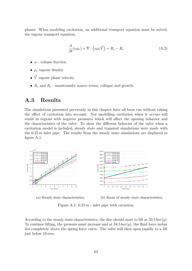
phases. When modeling cavitation, an additional transport equation must be solved,the vapour transport equation,

∂

∂t(αρv) +∇ ·

(αρv~V

)= Re −Rc (A.2)

• α - volume fraction

• ρv vapour denstiy

• ~V vapour phase velocity

• Rc and Re - masstransfer source terms, collapse and growth.

A.3 ResultsThe simulations presented previously in this chapter have all been run without takingthe effect of cavitation into account. Not modelling cavitation when it occurs willresult in regions with negative pressures which will affect the opening behavior andthe characteristics of the valve. To show the different behavior of the valve when acavitation model is included, steady state and transient simulations were made withthe 0.25m inlet pipe. The results from the steady state simulations are displayed infigure A.1.

0 1 2 3 4 5 6 7 8 9 10

0.7

0.8

0.9

1

1.1

1.2

1.3

1.4

1.5x 10

4

Lift (mm)

Fo

rce

(N

)

31 bar (g)

32 bar (g)

33 bar (g)

34 bar (g)

35 bar (g)

Spring

(a) Steady state characteristics.

0 0.1 0.2 0.3 0.4 0.5 0.6 0.7 0.8 0.9 1

7000

7200

7400

7600

7800

8000

8200

8400

8600

8800

9000

Lift (mm)

Fo

rce

(N

)

31 bar (g)

32 bar (g)

33 bar (g)

34 bar (g)

35 bar (g)

Spring

(b) Zoom of steady state characteristics.

Figure A.1: 0.25m - inlet pipe with caviation.

According to the steady state characteristics, the disc should start to lift at 33.5 bar(g).To continue lifting, the pressure must increase and at 34.5 bar(g), the fluid force isobarlies completely above the spring force curve. The valve will then open rapidly to a liftjust below 10mm.

63

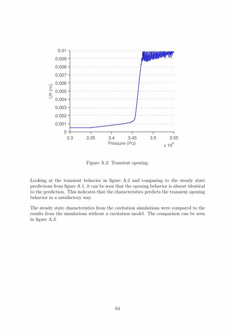
3.3 3.35 3.4 3.45 3.5 3.55

x 106

0

0.001

0.002

0.003

0.004

0.005

0.006

0.007

0.008

0.009

0.01

Pressure (Pa)

Lift

(m)

Figure A.2: Transient opening.

Looking at the transient behavior in figure A.2 and comparing to the steady statepredictions from figure A.1, it can be seen that the opening behavior is almost identicalto the prediction. This indicates that the characteristics predicts the transient openingbehavior in a satisfactory way.

The steady state characteristics from the cavitation simulations were compared to theresults from the simulations without a cavitation model. The comparison can be seenin figure A.3.

64

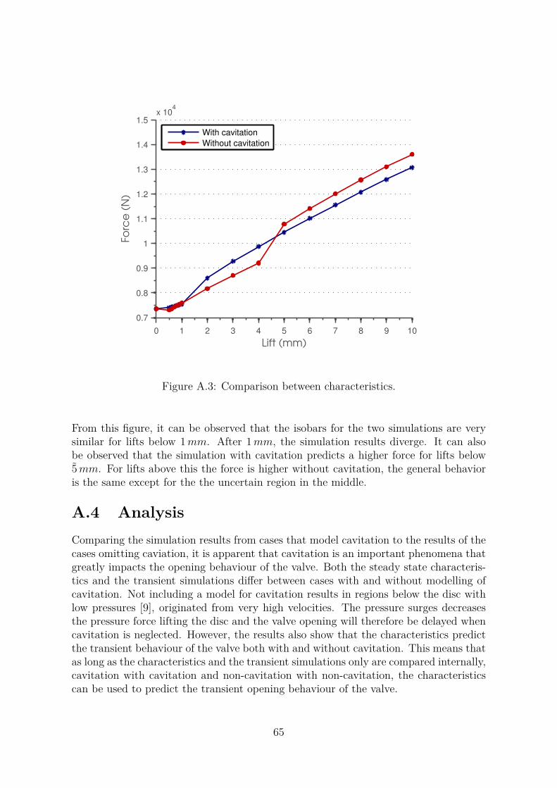
0 1 2 3 4 5 6 7 8 9 10

0.7

0.8

0.9

1

1.1

1.2

1.3

1.4

1.5

x 104

Lift (mm)

Fo

rce

(N

)

With cavitation

Without cavitation

Figure A.3: Comparison between characteristics.

From this figure, it can be observed that the isobars for the two simulations are verysimilar for lifts below 1mm. After 1mm, the simulation results diverge. It can alsobe observed that the simulation with cavitation predicts a higher force for lifts below5mm. For lifts above this the force is higher without cavitation, the general behavioris the same except for the the uncertain region in the middle.

A.4 AnalysisComparing the simulation results from cases that model cavitation to the results of thecases omitting caviation, it is apparent that cavitation is an important phenomena thatgreatly impacts the opening behaviour of the valve. Both the steady state characteris-tics and the transient simulations differ between cases with and without modelling ofcavitation. Not including a model for cavitation results in regions below the disc withlow pressures [9], originated from very high velocities. The pressure surges decreasesthe pressure force lifting the disc and the valve opening will therefore be delayed whencavitation is neglected. However, the results also show that the characteristics predictthe transient behaviour of the valve both with and without cavitation. This means thatas long as the characteristics and the transient simulations only are compared internally,cavitation with cavitation and non-cavitation with non-cavitation, the characteristicscan be used to predict the transient opening behaviour of the valve.

65

B. Orifice area

As mentioned in section 2.6 the authors of the article [7] came to the conclusion thatthe ratio between the orifice area and outlet area should be larger than 6.0 in order toavoid chatter. In this thesis the lenght of the two dimensional outlet area is 115,01mm.The valve opening ranges from 0.5mm to 9.86mm. The outlet and opening below thedisc will revlove around the axis and the the actual area will be the surface area.

r = AoutletAopening

≈ 40

The ratio is with a large margin in the safe region.

66

C. Numerical settings in FLUENT

In this section the settings used in FLUENT will be presented.

C.1 Turbulence model and boundary conditions• Turbulence model: SST-kω.

• Pressure inlet and pressure outlet for steady state simulations and transientsimulations of case 1.

• Velocity inlet and pressure outlet for transient simulations of case 2.

• No - slip conditions at walls.

C.2 Calculation schemesThe following numerical schemes were used for the simulations.

• Pressure - velocity coupling: Coupled.

• Momentum and Tubulent Kinetic Energy: QUICK.

• Density and Specific Dissipation Rate: 1st order upwind.

• Pressure: Standard.

• Gradient: Least Square based.

• Transient formulation: 1st order implicit (Only for transient simulations.).

C.3 Additional settingsHere, additional settings such as time-step, under relaxation factors and settings fordynamic mesh and mulitphase modelling will be presented.

67

Time step

The time-steps chosen for the transient simulations was 1ms, 0.1ms, 0.05ms and0.01ms. The choice of time-step for each simulation was based on the convergence, seesection C.4.

Under relaxation

• Flow Courant number = 20.

• Explicit relaxation factor for momentum = 0.75.

• Explicit relaxation factor for pressure = 0.75.

• All other under relaxation factors were set to Default.

Dynamic mesh

For the transient simulations, the following settings were used for the dynamic mesh;

• A constant αcollapse of 0.2.

• A constant αsplit of 0.4.

Multiphase modelling

For the simulations with cavitation modelling, the following settings were used;

• Multiphase model: Mixture model

• No slip - velocity between the phases.

• Incompressible vapour phase.

• Compressible liquid phase.

• Mass transfer from liquid phase to vapour phase.

• Default settings for modelling of the cavitation.

• Pressure- velocity coupling was set to Coupled - coupled with volume fractions.

• For steady state simulations, Pseudo-transient calculation with a time scale factorof 1 was chosen.

68

C.4 ConvergenceTo monitor the convergence for the steady state simulations the mass imbalance betweenthe inlet and outlet was observed, a value below 10−4 kg/s was considered low enough,however it was mostly lower. The drag at the disc boundary was also monitored andwhen reached a constant value.

To monitor the convergence for the transient simulation, the mass imbalance for each it-eration within a timestep was checked. The number of iterations used within a timestepwas chosen high enough to reach a constant value of the mass imbalance between theinlet and outlet.

69

Bibliography

[1] Bengt Andersson and dawsonera (e-book collection). Computational fluid dynamicsfor engineers. Cambridge University Press, Cambridge, 2012.

[2] J.L Garcia B. Ziegler, P. Coppolani. Dynamic behavior of check valves and safetyvalve with fluid interaction. Nuclear Engineering and Design, 124(1):391–401, 1990.10.1115/1.4006904.

[3] J. Cremers and L. Friedel. Design of spring loaded safety valves with inlet anddischarge pipe against chatter in the case of gas flow. Chemical Engineering &Technology, 26(5):573–576, 2003.

[4] Ron Darby. The dynamic response of pressure relief valves in vapor or gas service,part i: Mathematical model. Journal of Loss Prevention in the Process Industries,26(6):1262 – 1268, 2013.

[5] O. Frommann and L. Friedel. Analysis of safety relief valve chatter induced bypressure waves in gas flow. Journal of Loss Prevention in the Process Industries,11(4):279–290, 1998.

[6] ANSYS INC. Fluent 14.5 user guide.

[7] Hisao Izuchi. Stability analysis of safety valve, 2010.

[8] Robert T. Knapp, Frederick G. Hammitt, and James W. Daily. Cavitation.McGraw-Hill, New York, 1970.

[9] Vasilios Kourakos, Patrick Rambaud, Jean-Marie Buchlin, and Said Chabane.Flowforce in a safety relief valve under incompressible, compressible, and two-phase flow conditions. Journal of Pressure Vessel Technology, 135(1):11305, 2013.

[10] Kollika NGUON, Kazuaki INABA, Hiroto TAKAHASHI, and Kikuo KISHI-MOTO. Numerical study on wave propagation in coupled pipe and homogeneoussolid-liquid flow. Theoretical and Applied Mechanics Japan, 60:239–248, 2012.

[11] Smith, D. Burgess, J. Powers, and C. Relief device inlet piping: Beyond the 3percent rule, 2011.

[12] A.S. Tijsseling. Fluid-structure {INTERACTION} {IN} liquid-filled {PIPE} sys-tems: A {REVIEW}. Journal of Fluids and Structures, 10(2):109 – 146, 1996.

70

[13] Lurton Xavier. An introduction to Underwater Acoustics Principles and applica-tions. Springer, 2010.

71

On the Stability of Pressure Relief...

Documents

Transcript of On the Stability of Pressure Relief...