On the Simple Economics ofAdvertising, Marketing, and Product Design

Justin P. Johnson

Johnson Graduate School of Management, Cornell University

jpj25@cornell.edu

David P. Myatt

Department of Economics and St. Catherine’s College, Oxford University

david.myatt@economics.ox.ac.uk

August 2004.1

Oxford University Economics Discussion Paper 185.

We propose a framework for analyzing transformations of the demand facing a mo-nopolist. Our approach is based on the observation that such transformations fre-quently stem from changes in the dispersion of consumers’ valuations, which lead torotations of the demand curve. In a wide variety of settings, profits are a U-shapedfunction of dispersion. The monopolist will adopt a mass-market posture when dis-persion is low, and a niche posture when dispersion is high. We investigate numerousapplications of our framework, including product design and development; adver-tising, marketing and sales advice; and the construction of quality-differentiatedproduct lines. We also suggest a new taxonomy of advertising, distinguishing be-tween hype, which shifts demand, and real information, which rotates demand.

1. Shaping Consumer Demand

The shape of the demand curve for a product is fundamental to the behavior and profitabil-

ity of a supplier. Demand is influenced by many factors, some of which are exogenous, such

as consumers’ incomes and preferences, and others of which are endogenous. For instance,

advertising, marketing, and product design are all activities that shape demand. Here we

develop an approach to analyzing the changing demand for a monopolist’s product that is

broadly applicable and yet easily understood in terms of basic economic concepts. This

approach stems from the observation that demand-shaping activities often change the dis-

persion of consumers’ valuations, which leads not to a shift but rather to a rotation of the

demand curve.

To motivate our study, first consider an alteration to a product’s original design. If consumers

unanimously prefer the new version then the consequences are simple: The demand curve

shifts outward, so that for any given quantity, revenue must increase. Thus, a monopolist

will modify the design unless there are countervailing factors such as an increase in costs.

1We thank seminar participants, especially Meg Meyer and Paul Klemperer, for helpful comments.

2

In other situations, product design is less straightforward. For example, a design change

may appeal to some consumers, while displeasing others. Often this will correspond to a

change in the dispersion of demand (by which we mean an increase in the dispersion of the

distribution of consumers’ willingness-to-pay) rather than a simple shift.

As further motivation, consider advertising and marketing activities. If product promotion

is unambiguously persuasive, or informs consumers of a product’s existence, then it will

shift the demand curve outward. As with product design, however, the effects may be

more complex. This will be so when advertising provides pre-sales information that enables

consumers to better ascertain their true underlying idiosyncratic preferences for the product.

For instance, a marketing campaign may provide many details of a product’s style and

function, or it may simply hype the product’s existence. Providing detailed information may

discourage some customers from purchasing while encouraging others. Thus, the consequence

of providing information is an increase in the dispersion of demand.

Our approach encompasses such situations in which the shape of a demand curve is deter-

mined by the dispersion of consumers’ willingness-to-pay. While this analysis is somewhat

more subtle than that involving mere shifts in demand, the end results nonetheless turn out

to be fairly straightforward. The reason is that an increase in dispersion frequently induces

a clockwise rotation of the demand curve. Therefore, understanding the simple economics of

demand rotation suffices to comprehend the motivations for a monopolist to mold demand

(or to understand responses consequent to an exogenous demand transformation) in a variety

of settings. Thus we consider a family of demand curves indexed by a sequence of clockwise

rotations, and investigate the effect of increased dispersion.

When consumers’ valuations for the product are relatively homogeneous, the demand curve

will be relatively flat. Typically, a monopolist will choose to serve a large fraction of potential

consumers. Heuristically, the marginal consumer is “below average” in the distribution of

valuations. Following an increase in dispersion, the demand curve rotates clockwise. This

will push the willingness-to-pay of the marginal consumer down, and monopoly profits will

fall. Eventually, the steepening demand curve will prompt the monopolist to restrict sales

to a relatively small fraction of potential consumers. The marginal consumer will then be

“above average” and respond positively to increases in dispersion; monopoly profits increase

as the demand curve rotates clockwise. Building upon this intuition we show that, in a

wide variety of circumstances, monopoly profits are “U-shaped” (that is, quasi-convex) in

the dispersion of demand. Such profits achieve a maximum when the dispersion is either

maximized or minimized. Consequently, a monopolist will wish to use any tools at her

disposal, such as her advertising and product-design decisions, to pursue one of these two

extremes. We identify, therefore, two distinct marketing mixes that the monopolist may

wish to deploy.

3

First, the monopolist may stake out a “mass market” position, in which her product is sold

to many consumers. In this case, her goal is to minimize the dispersion of demand. In pursuit

of this goal, the product will be designed to have universal appeal, with controversial design

features being eschewed; it will offer something for everyone. Any advertising will highlight

the existence of the product, but will not allow consumers precisely to learn of their true

match with the product’s characteristics. Such a marketing mix will ensure that consumers

share similar valuations for the product, so that we will see a “plain vanilla” product design

promoted by an advertising campaign consisting of “pure hype.”

Second, the alternative is the adoption of a “niche” position, where few units are sold. The

monopolist aims to maximize the dispersion of demand. The product design will have ex-

treme characteristics that appeal to specialized tastes; it will pander to the highest extreme.

Many consumers will strongly dislike the product, but those who like it will love it. This

product design will be accompanied by advertising and detailed sales advice containing “real

information” that allows consumers to learn of their true match with the product’s attributes.

A number of applications flow from our basic observation that many factors influence the

shape of demand. For instance, building upon the intuition above, we introduce a new tax-

onomy of advertising, distinguising between hype and real information. Promotional hype

corresponds to the traditional notions of informative and persuasive advertising. It high-

lights the existence of the product, promotes any feature that is unambiguously valuable,

or otherwise increases the willingness-to-pay of all consumers; it shifts the demand curve

outward. Real information, on the other hand, allows a consumer to learn of his personal

match with the product’s characteristics; as we show, it rotates the demand curve. Employ-

ing this taxonomy, we study an advertising life-cycle in which a monopolist’s choice of both

the intensity of an advertising campaign and its real-information content change over time

in response to consumer learning. We also examine the decision to introduce an improved

version of an existing product, and relate this to issues such as the existing stock of consumer

knowledge regarding the brand. Furthermore, we are able to ascertain the response of these

decisions to other endogenous variables, such as the product’s design, as well as exogenous

variables, such as inequality in the income distribution.

Our results are not artifacts of an assumption that a monopolist sells but a single product:

We extend our analysis to a multiproduct monopolist offering a product line of vertically

differentiated goods. In this setting a consumer’s type corresponds to a preference for in-

creased quality, and monopoly profits are U-shaped in the dispersion of such types. We

also present a number of comparative statics relating the length and mix of a product line

to consumer-type dispersion. For instance, when types are more disperse a monopolist will

tend to serve a smaller overall share of the market, but do so with more products.

4

Our work is related to several distinct fields of economic inquiry. We believe that fully con-

veying such relationships is best accomplished by deferring thorough review to the individual

subsequent sections. However, a few notes are in order here. In Section 2, we investigate the

response of a single-product monopolist’s profits and output to the dispersion of demand.

Our notion of dispersion builds upon the classic work of Rothschild and Stiglitz (1970, 1971)

and the single-crossing property of distribution functions studied by Diamond and Stiglitz

(1974) and Hammond (1974). In Section 3 we apply our theory to product design and

development. Our approach to product design is based upon Lancastrian (1966, 1971) char-

acteristics, and the analysis of product development is assisted by a result of Jewitt (1987).

In Section 4 we turn to advertising, sales advice and other marketing activities. Our study

of the incentives to equip consumers with private information exploits the insights of Lewis

and Sappington (1991, 1994), and complements Ottaviani and Prat’s (2001) work on public

information supply. Section 5’s consideration of a multiproduct monopolist selling vertically

differentiated goods builds upon the classic Mussa-Rosen (1978) model.

Taken together, a fundamental point emerging from our results is that demand-transforming

events interact with a broad array of decision variables, so that reaching a better understand-

ing of these events is critical to understanding a firm’s overall activities. Equally important

is that studying changes in the dispersion of demand frequently reduces to the study of sim-

ple rotations of demand, so that basic economic intuition is all that is required to explore a

range of issues including advertising, marketing, and product design.

2. Demand Dispersion and a Monopolist’s Preference for Extremes

Our goal here is to provide the core theoretical framework upon which we build in later

sections. We consider a scenario in which a monopolist sells a single product, and investigate

the relationship between the shape of the distribution of consumers’ willingness-to-pay and

the monopolist’s profits, quantity, and price.

2.1. A Single-Product Monopoly Model. A single-product monopolist serves a unit

mass of consumers, each of whom has (at most) unit demand for her product. An individual

consumer’s type θ ∈ R is his valuation, or his willingness-to-pay, for a single unit: Facing a

price of p ≥ 0, he demands a single unit of the product if and only if θ > p. The type θ does

not necessarily represent a consumer’s true payoff (in monetary terms) from consumption:

At the time of purchase, a consumer might well be uncertain of either the product’s precise

attributes, or indeed his own tastes. Our interpretation is that θ represents the certainty

equivalent of the lottery obtained from a purchase. Thus, if a consumer is risk-neutral, then

θ is his expected monetary valuation for a single unit of the product. On the cost side, if

the monopolist supplies z units then she incurs costs of C(z).

5

We consider a family of distributions {Fs(θ)} indexed by s ∈ S = [sL, sH ] ⊆ R. For a

particular s, types are drawn from Fs(θ), with support on some open interval of R. Fs(θ) is

twice continuously differentiable in θ and s, and fs(θ) is its strictly positive density.

Fixing s, Fs(θ) yields a demand curve: At a price of p, z = 1−Fs(p) consumers will purchase,

yielding revenue of p(1−Fs(p)). At times, we will find it convenient to view the monopolist

as setting quantity rather than price. To this end, we write Ps(z) for the type (or willingness-

to-pay) of the consumer with a mass z of others above him. Hence, if the monopolist wishes

to sell z units, then she must set a price of p = Ps(z). Thus Ps(z) is the inverse-demand

curve, and must satisfy z = 1−Fs(Ps(z)), or equivalently Ps(z) = F−1s (1−z). We write π(s)

for the monopolist’s maximized profits given a consumer-valuation distribution Fs(θ). When

uniquely defined (for instance, when marginal revenue is decreasing and costs are convex)

we write z∗s for the monopoly quantity and p∗s for the monopoly price:

π(s) = maxz∈[0,1]

{zPs(z)− C(z)}, z∗s = arg maxz∈[0,1]

{zPs(z)− C(z)}, and p∗s = Ps(z∗s).

2.2. Indexing the Shape of Consumer Demand. Exogenous shifts in the environment,

and actions taken by the monopolist, the consumers, or some third party, may all influence

the distribution Fs(θ) (equivalently, the demand curve) faced by the monopolist, and hence

her profitability. An exploration of this relationship between the nature of demand and

profitability requires a comparison of Fs(θ) and Fr(θ) for r, s ∈ S. If Fs(θ) is higher than

Fr(θ) in the sense of strict first-order stochastic dominance (following classic definitions,

such as that of Lehmann (1955), so that Fs(θ) < Fr(θ) for all θ) then the inverse-demand

curve shifts up from Pr(z) to Ps(z), and the monopolist’s profits must increase. For instance,

if the monopolist benefits from a product innovation that is unambiguously valued by all

consumers, then her profits will rise. Similarly, if advertising (perhaps the promotion of a

product innovation) convinces all consumers of the product’s merits, then profits again will

be higher (putting aside potential changes in the cost structure).

Simple shifts in demand, however, are not our primary focus. We wish to consider the shape

of the demand curve, and in particular situations in which Fs(θ) is “more disperse” or “more

heterogeneous” than Fr(θ).2 For instance, and as discussed in Section 1, a modification

to the product’s design may increase the valuation of some consumers, while reducing the

valuation of others. Similarly, advertising or sales advice may convince some consumers of

the product’s merits, while persuading others that the product does not meet their needs. We

consider concrete examples of these scenarios in Sections 3–4. For our preliminary analysis,

however, we require a measure of “riskiness” to rank different distributions.3

2Our distinction is motivated by Atkinson’s (1970, p. 245) suggestion to “separate shifts in the distributionfrom changes in its shape and confine the term inequality to the latter aspect.”3There is no uncertainty over the demand curve faced by the monopolist; our work is distinct from that ofLeland (1972) and Coes (1977) who considered a risk-averse firm faced by a stochastic demand curve.

6

0 1 2 3 4

Consumer Valuation θ

..............................................................................................................

r

s

........

........

........

........

........

........

........

........

.................

...............

........

........

........

................

....................•

θsr..........•

θsr

............. ............. ............. fr(θ)

................................................................fs(θ)

............. ............. .............................................................................................................................................................................................................................

.........................................................................................................................................................................

.......................... ............. ............. ............. .............

......................................

...............................

...........................................................................................................................................................................

.....................................

.......................................................................................................................................................................................................................................................................................................................................................

(a) Density Functions fr(θ) and fs(θ)

0 1 2 3 4

Consumer Valuation θ

........

........

.......................

...............

..........................................................................................

.

.

.

.

.

.•

θ†sr

............. ............. .............Fr(θ)

................................................................Fs(θ)

............. ............. ............. ............. ..........................

...................................................................................................................................................................................................

............. ............. ............. ............. ............. ............. .............

.................................................................

........................................

...............................

..................................................................................................................................................................................................................................................................................................................................................................................................

...................................

.............................................

................................................

(b) Distribution Functions Fr(θ) and Fs(θ)

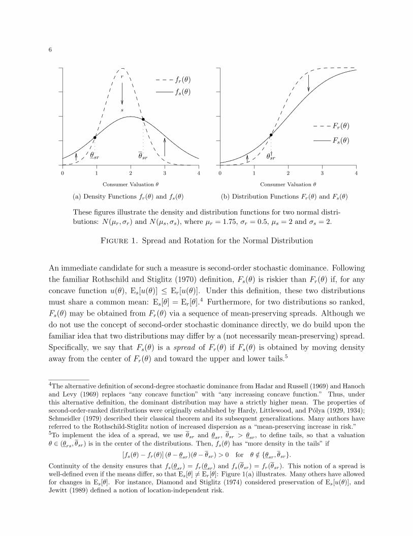
These figures illustrate the density and distribution functions for two normal distri-butions: N(µr, σr) and N(µs, σs), where µr = 1.75, σr = 0.5, µs = 2 and σs = 2.

Figure 1. Spread and Rotation for the Normal Distribution

An immediate candidate for such a measure is second-order stochastic dominance. Following

the familiar Rothschild and Stiglitz (1970) definition, Fs(θ) is riskier than Fr(θ) if, for any

concave function u(θ), Es[u(θ)] ≤ Er[u(θ)]. Under this definition, these two distributions

must share a common mean: Es[θ] = Er[θ].4 Furthermore, for two distributions so ranked,

Fs(θ) may be obtained from Fr(θ) via a sequence of mean-preserving spreads. Although we

do not use the concept of second-order stochastic dominance directly, we do build upon the

familiar idea that two distributions may differ by a (not necessarily mean-preserving) spread.

Specifically, we say that Fs(θ) is a spread of Fr(θ) if Fs(θ) is obtained by moving density

away from the center of Fr(θ) and toward the upper and lower tails.5

4The alternative definition of second-degree stochastic dominance from Hadar and Russell (1969) and Hanochand Levy (1969) replaces “any concave function” with “any increasing concave function.” Thus, underthis alternative definition, the dominant distribution may have a strictly higher mean. The properties ofsecond-order-ranked distributions were originally established by Hardy, Littlewood, and Polya (1929, 1934);Schmeidler (1979) described their classical theorem and its subsequent generalizations. Many authors havereferred to the Rothschild-Stiglitz notion of increased dispersion as a “mean-preserving increase in risk.”5To implement the idea of a spread, we use θsr and θsr, θsr > θsr, to define tails, so that a valuationθ ∈ (θrs, θsr) is in the center of the distributions. Then, fs(θ) has “more density in the tails” if

[fs(θ)− fr(θ)] (θ − θsr)(θ − θsr) > 0 for θ /∈ {θsr, θsr}.Continuity of the density ensures that fs(θsr) = fr(θsr) and fs(θsr) = fr(θsr). This notion of a spread iswell-defined even if the means differ, so that Es[θ] 6= Er[θ]: Figure 1(a) illustrates. Many others have allowedfor changes in Es[θ]. For instance, Diamond and Stiglitz (1974) considered preservation of Es[u(θ)], andJewitt (1989) defined a notion of location-independent risk.

7

When Fs(θ) is a spread of Fr(θ), the two distributions must cross at a single point θ†sr.

This is the center of the spread exercise: For θ < θ†sr, weight is pushed down into the lower

tail, so that Fs(θ) > Fr(θ); for θ > θ†sr, weight is pushed up into the upper tail, so that

Fs(θ) < Fr(θ). We call θ†sr the rotation point of the spread, since the cumulative distribution

function “rotates” around it.6 Figure 1(b) illustrates this effect. We may also consider local

changes in s, which may yield a local spread of the distribution Fs(θ).7 For such a local

spread, there is some rotation point θ†s such that Fs(θ) is increasing in s for θ < θ†s, and

decreasing in s for θ > θ†s. In fact, a rotation is a weaker measure of increased dispersion

than a spread.8 It is central to our analysis, and hence we state it as a formal definition.

Definition 1. Fs(θ) is a rotation of Fr(θ) if, for some rotation point θ†sr,

[Fs(θ)− Fr(θ)] (θ − θ†sr) < 0 for θ 6= θ†sr.

A local change in s leads to a local rotation of Fs(θ) if, for some rotation point θ†s,

∂Fs(θ)

∂s(θ − θ†s) < 0 for θ 6= θ†s.

If this holds for all s ∈ S, then {Fs(θ)}s∈S is ordered by a sequence of local rotations.

Definition 1 stipulates that two cumulative distribution functions, differing by a (clockwise)

rotation, must cross only once. Employing this notion, Diamond and Stiglitz (1974) de-

scribed the difference between distributions as satisfying a single-crossing property, whereas

Hammond (1974) defined the corresponding random variables to be simply intertwined. It is

well known that such a relationship corresponds to an increase in riskiness in the following

sense: If, for some increasing function u(θ), Es[u(θ)] ≤ Er[u(θ)], and v(θ) is more risk-averse

than u(θ) in the sense of Arrow (1970) and Pratt (1964), then Es[v(θ)] < Er[v(θ)].9

6In Section 1 we used the terms “below average” and “above average” to describe a marginal consumer.When comparing Fr(θ) and Fs(θ) the “average consumer” has type θ = θ†sr.7Since s is drawn from the interval S = [sL, sH ], and Fs(θ) is continuously differentiable, local changes in smay be considered. We say that such a change leads to a local spread of Fs(θ) if, for some θs < θs,

∂fs(θ)∂s

(θ − θs)(θ − θs) > 0 for θ /∈ {θs, θs},

where, once again, continuity ensures that ∂fs(θs)/∂s = ∂fs(θs)/∂s = 0.8For a rotation, the distribution functions cross once. Their densities, however, may cross an arbitrarynumber of times. If they differ by a spread, then their densities will cross only twice. Although we restrictour analysis to rotations throughout the paper, our results (particularly Proposition 1) do extend to measuresof increased dispersion that involve multiple rotation points; we return to this issue later in the paper.9Formally, v(θ) is a concave transformation of u(θ) and hence displays a higher coefficient of absolute risk-aversion. Then, if an agent with utility function u(θ) prefers the distribution Fr(θ), then so will the (morerisk-averse) agent with utility function v(θ). This result has been proved independently by a number ofdifferent authors. It was the focus of Hammond’s (1974) paper, appeared as a lemma in Grossman and Hart(1983, p. 151), and formed a basis for the contributions of Jewitt (1987, 1989).

8

Henceforth in this section, we will assume that the family {Fs(θ)}s∈S is ordered by a se-

quence of local rotations.10,11 It follows that the associated family of inverse-demand curves

{Ps(z)}s∈S is also ordered by a sequence of local rotations; for each s there is a rotation

quantity z†s ∈ [0, 1] that satisfies z†s = 1− Fs(θ†s), and

∂Ps(z)

∂s(z − z†s) < 0 for z 6= z†s.

Thus a local increase in s results in a clockwise rotation of the inverse-demand curve around

the quantity-price pair of z = z†s and p = θ†s. This ensures that the inverse-demand curve

becomes steeper, and hence less elastic, when evaluated at the rotation quantity z†s.12

A special case of the local-rotation ordering is obtained when we consider a family of distri-

butions that are indexed by scale and location parameters: An increase in dispersion then

corresponds to an increase in variance. We employ the following definition.13

Definition 2. The family {Fs(θ)}s∈S is ordered by a sequence of mean-variance shifts if,

for some distribution F (θ) with zero mean, unit variance, and density f(θ) > 0,

Fs(θ) = F

(θ − µ(s)

σ(s)

),

where µ(s) and σ(s) are continuously differentiable, σ(s) > 0 and σ′(s) > 0.

10Note that we do not require any two distinct members, Fs(θ) and Fr(θ), to be ordered by a rotation. Ofcourse, if θ†s = θ† for all s, then any pair of distributions Fr(θ) and Fs(θ) do differ by a rotation. Furthermore,even if θ†s is not constant, we may rank Fr(θ) and Fs(θ) in their upper and lower tails. Formally, if r < s,

θ < infs′∈[r,s]

θ†s′ ⇒ Fr(θ) < Fs(θ), and θ > sups′∈[r,s]

θ†s′ ⇒ Fr(θ) > Fs(θ).

Definition 1 insists that Fr(θ) and Fs(θ) cross at some point θ†sr. We could, of course, weaken this bypermitting pairs of distributions that do not cross, and hence are ordered by first-order stochastic dominance;this would be accomplished by allowing θ†sr to take values outside the support of θ. Hammond (1974) allowedfor distributions that are either simply intertwined (this differs slightly from our definition, by allowing fordistributions that coincide on some interval) or first-order-dominance ranked. When one of these orderingsholds, the distributions are “simply related.” Hammond (1974, p. 1069) observed that many families ofdistributions have members that are all simply related, including the (separate) families of uniform, normal,geometric, exponential, gamma and beta distributions.11When all distributions in the family share a common mean, a local-rotation ordering is sufficient to ensurethat any distinct pair of distributions are ordered by second-order stochastic dominance. A partial converseis also true. For instance, suppose that, for a finite set S, distributions are ordered by second-order stochasticdominance. Following Rothschild and Stiglitz (1970) and Machina and Pratt (1997), we may construct asequence of mean-preserving spreads (and hence rotations) linking each pair. In such a manner, we mayobtain an (expanded) family of distributions ordered by a sequence of local rotations.12If we were to specify a family of demand curves index by decreasing elasticity, then we would need tospecify whether the elasticities of two curves are to be compared at a common quantity, or a common price.Whatever the convention adopted, if Ps(z) to be less elastic than Pr(z) then it must be steeper wheneverthe demand curves cross. This further implies that they must cross only once. Thus an elasticity-orderedfamily of demand curves must be ordered by a sequence of local rotations.13If a family is ordered by a sequence of local rotations, then the distributions of any increasing transformationof θ are so ordered. Hence Definition 2 could be weakened, while retaining many of our results, by allowingfor distributions corresponding to an increasing transformation of θ to satisfy the definition.

9

0.00 0.25 0.50 0.75 1.00

Quantity z

........

........

........

........

........

...................

...............

..........................................................

............. ............. ............. ............. ............. ............. ............. ............. ............. ............. ............. ............. ............. ............. ............. ............. ............. s = 14

..................................................................................................................................................................................................................................................................................................................................................................................................................................................................................... s = 2

(a) Rotating Inverse-Demand Ps(z)

0 1 2 3 4

Standard Deviation of Valuations s

.

.

.

.

.

.

.

.

.

.

.

.

.

.

.

.

.

.

.

.

.

.

.

.

.

.

.

•

s

z∗s > z†s

π′(s) < 0

(Mass Market)

z∗s < z†s

π′(s) > 0

(Niche)

z†s

z∗s

............. ............. ............. ............. ............. ............. ............. ............. ............. ............. ............. ............. ............. ............. ............. ............. ............. ............. .....

..................................................................................................................................................................................................................................................................................................................................................................................................................................................................................................................................................

(b) z∗s versus z†s

These figures illustrate the rotation of the inverse-demand function Ps(z) and therelative size of the monopoly quantity z∗s and rotation quantile 1− z†s. The specifi-cation is θ ∼ N(µ(s), s2), where µ(s) = 2.45 + 0.05s2.

Figure 2. Inverse-Demand Rotation and Niche versus Mass-Market

Thus Fs(θ) has a mean of µ(s), a standard deviation of σ(s), and inverse-demand

Ps(z) = µ(s) + σ(s)P (z),

where P (z) = F−1(1 − z). Insisting that σ′(s) > 0 ensures that the family is ordered by a

sequence of local rotations.14 Since σ′(s) > 0 is required, it is without loss of generality to

set σ(s) = s when convenient, yielding the inverse-demand function Ps(z) = µ(s) + sP (z).

Many specifications meet the requirements of Definition 2. For instance, a family of normal

distributions (from which the illustrations of Figure 1 are taken) does so.

2.3. Quasi-Convexity of Profits and a Preference for Extremes. We turn now to

consider the response of the monopolist’s profits to changes in the dispersion index s. We have

noted that, from a quantity-setting perspective, her inverse-demand curve rotates clockwise

around z†s following a local increase in s.15 If the monopolist supplies z units then, for z < z†s,

the price received is increasing in s. For z > z†s, it is decreasing in s.

A straightforward intuition is that, for z∗s > z†s, the monopolist acts as a “mass market”

supplier. By supplying more than z†s, she ensures that the marginal consumer, with type

θ = p∗s = Ps(z∗s), lies below the rotation point θ†s. An increase in s pushes consumers away

14It is straightforward to show that the rotation point satisfies θ†s = µ(s)− σ(s)µ′(s)/σ′(s). When σ(s) = sthis simplifies to θ†s = µ(s)− sµ′(s), and the rotation quantity satisfies z†s = 1− F (−µ′(s)).15The term “demand rotation” was used by Aislabie and Tisdell (1988), who related the slope to marketingdecisions. They referred to flat and steep demand curves as “bandwagon-type” and “snob-type” respectively.

10

from θ†s. Hence, it pushes the type (and willingness-to-pay) of the marginal consumer down.

Since the price is determined by the identity of the marginal consumer, and not the average

consumer, both the price and profits fall. In contrast, when z∗s < z†s, the monopolist acts

as a “niche” operator, by restricting supply to a smaller fraction of the potential consumer

base. The same logic ensures that profits increase with s. Employing the envelope theorem,

∂π(s)

∂s(z∗s − z†s) < 0 for z∗s 6= z†s.

This does not suffice to characterize the effect of increases in s across the entire interval S,

since the sign of (z∗s − z†s) might well change a number of times. There is, however, a simple

sufficient condition that ensures that the sign changes at most once.16

Proposition 1. Suppose that the family of distributions {Fs(θ)}s∈S is ordered by a sequence

of local rotations. Further suppose that the rotation point θ†s is decreasing in s, or equivalently

that the rotation quantity z†s is increasing in s. Then π(s) is a quasi-convex function of s.

maxs∈S π(s) ∈ {π(sL), π(sH)}, and hence the monopolist prefers the extremes sL and sH .

Quasi-convex profits are highest when consumers’ valuations are either as heterogeneous

as possible, or as homogeneous as possible. If the monopolist were able to choose s, then

she would take either an extreme niche posture (by setting s = sH) or an extreme mass-

market posture (the opposite extreme of s = sL). Furthermore, as either sL or sH increase,

π(sH)− π(sL) crosses from negative to positive at most once.

Proposition 1 follows from the observation that, as s rises, the monopolist will never switch

from a niche position to a mass-market position. If she were to do so, then we could find

an interval [s′, s′′] ⊆ S such that z∗s′ < z†s′ ≤ z†s′′ < z∗s′′ . As s rises from s′ to s′′, the rotation

quantity z†s increases, and hence ∂Ps(z∗s′)/∂s > 0 throughout. Similarly, ∂Ps(z

∗s′′)/∂s < 0

over the same interval. But this implies that, for s = s′′, a supply of z∗s′ is strictly more

profitable than a supply of z∗s′′ . This is a contradiction. It follows that the monotonicity

of z†s is sufficient (but not necessary) to guarantee that once s is sufficiently large to make

a niche operation optimal, the monopolist will never wish to switch back to mass-market

supply. This ensures that π′(s) remains positive for all larger s, and π(s) is a quasi-convex

(hence either monotonic or “U-shaped”) function.17

Monotonicity of z†s (equivalently, θ†s) is straighforward to check. If z < z†s, then ∂Ps(z)/∂s >

0, so that the price is locally increasing in s. Since z†s is increasing, the same is true for

16Proofs omitted from the text are contained in Appendix A.17Figure 2 illustrates this result, where Fs(θ) is drawn from a family of normal distributions. Consider ans such that z∗s − z†s = 0. As s increases, the clockwise rotation steepens the demand curve, and hencereduces the elasticity. This reduction in elasticity implies that the monopoly quantity z∗s moves down. Byassumption, z†s is increasing. It follows that z∗s − z†s must cross zero at most once, and from above. Thiscrossing (if it occurs) is the single transition from mass-market to niche supply.

11

larger s. Thus, fixing z, ∂Ps(z)/∂s > 0 crosses zero at most once, and this must be an

upcrossing. Equivalently, the price Ps(z) is, for fixed z, a quasi-convex function of the

dispersion parameter s. This observation forms part of the following lemma.

Lemma 1. When the family {Fs(θs)}s∈S is ordered by a sequence of local rotations,

(1) θ†s is a decreasing function of s,

(2) z†s is an increasing function of s,

(3) Fs(θ) is a quasi-concave function of s for all θ, and

(4) Ps(z) is a quasi-convex function of s for all z,

are all equivalent statements. Further, if the family is ordered by a sequence of mean-variance

shifts, then (i)–(iv) hold if and only if µ′(s)/σ′(s) is weakly increasing in s.

For a family of distributions ordered by a sequence of mean-variance shifts (Definition 2) the

requirement that µ′(s)/σ′(s) be weakly increasing is equivalent to the inequality µ′′(s)σ′(s) ≥µ′(s)σ′′(s).18 Of course, in the mean-variance shift case, we may set σ(s) = s without loss,

and reduce the final statement of Lemma 1 to µ′′(s) ≥ 0: As we move through the variance-

ordered family of distributions, the mean is a convex function of the standard deviation.

As we show subsequently, the conditions of Lemma 1 are satisfied for many applications.

Furthermore, an alternative proof of Proposition 1 follows from the observations that (i)

Lemma 1 applies, so that Ps(z) is quasi-convex in s, and (ii) π(s) = maxz∈[0,1]{zPs(z)−C(z)}is the maximum of quasi-convex functions, and so is itself quasi-convex.19

2.4. Niche versus Mass-Market Operation. In the previous section we categorized a

monopolist’s posture as either being a niche or a mass-market one, depending on whether

she is serving fewer or more than z†s consumers, respectively. Here we continue to make use

of this distinction, and show how it is useful in categorizing the change in the monopolist’s

optimal output z∗s in response to shifts in s.

Detailed comparative statics require more structure than that possessed by an arbitrary

family of demand curves ordered by local rotations. The reason is that such comparative

statics depend on properties of marginal revenue, and the rotation ordering is broad enough

18If µ(s) is increasing, then this inequality is equivalent to −µ′′(s)/µ′(s) ≤ −σ′′(s)/σ′(s), which says thatµ(s) is less concave than σ(s), in the Arrow (1970) and Pratt (1964) sense.19Notice that this proof applies even when the family of distributions is not ordered by a sequence of localrotations. As suggested in Footnote 8, Lemma 1 and Proposition 1 may be modified to cope with moregenerality. Exploring this, notice that for a family ordered by a sequence of local rotations, θ†s the is onlyvaluation at which demand is stationary (to first order) in response to a local change in s. More generally,there may be many such points. We can subdivide such rotation points into an ordered, alternating, sequenceof two types: Clockwise rotation points (the inverse-demand curve steepens with s), and anti-clockwiserotation points (inverse-demand becomes shallower with s). For quasi-convexity of profits, we require anyclockwise rotation to be decreasing, and any anti-clockwise rotation point to be increasing.

12

to impose few restrictions on the dependence of marginal revenue on s. Therefore, we

specialize to the case of mean-variance shifts (Definition 2), taking σ(s) = s and µ′′(s) ≥ 0

so that Proposition 1 holds. We also assume that C(z) is convex and differentiable, and that

Ps(z) exhibits decreasing marginal revenue. Note that, since Ps(z) = µ(s)+ sP (z), marginal

revenue is given by

MRs(z) = Ps(z) + zP ′s(z) = µ(s) + s [P (z) + zP ′(z)] = µ(s) + sMR(z),

where MR(z) is the marginal revenue associated with the inverse-demand curve P (z). Thus,

Ps(z) exhibits decreasing marginal revenue exactly when MR(z) is decreasing, i.e., whenever

the foundational inverse-demand curve P (z) exhibits decreasing marginal revenue.

This common assumption of decreasing marginal revenue MR(z) turns out to have powerful

consequences in this setting. It ensures that increases in s correspond to clockwise rotations

not only of the inverse-demand curve Ps(z), but also of the marginal revenue curve MRs(z).

This in turn generates a number of other results, summarized in the following proposition.

Proposition 2. Suppose that the family of distributions is ordered by a sequence of mean-

variance shifts, so that Fs(θ) = F ((θ − µ(s))/s), that µ(s) is convex, and that P (z) =

F−1(1−z) exhibits decreasing marginal revenue. Then π(s) is convex in s, and the monopoly

supply z∗s is quasi-convex in s. Furthermore, marginal revenue satisfies:

(1) A local increase in s rotates marginal revenue clockwise around some z‡s ∈ [0, 1],

(2) for each z, marginal revenue is convex in s,

(3) z‡s is increasing in s and satisfies z‡s < z†s, and

(4) the rotation point of marginal revenue MR‡s = MRs(z

‡s) is weakly decreasing in s.

Turning back to the monopoly supply z∗s , and for a constant marginal cost c,

(5) if c > MR‡sL

then z∗s is increasing for all s,

(6) if c < MR‡sH

then z∗s is decreasing for all s,

(7) otherwise z∗s is non-monotonic, and minimized for interior s ∈ (sL, sH). Finally,

(8) if µ(s) = µ for all s, then z∗s is increasing for µ > c, and decreasing for µ < c.

Because marginal revenue rotates (clockwise) around some rotation quantity z‡s as s increases,

comparative statics on the monopoly output depend on whether MR‡s = MRs(z

‡s) is above

or below marginal cost.20 Since z‡s < z†s, this is in turn connected to whether the monopolist

is adopting a niche or a mass-market posture. This is easiest to see when there is a constant

marginal cost, and so we suppose for discussion purposes that C(z) = cz.

20Proposition 2 allows marginal revenue to “rotate” around z‡s = 0 or z‡s = 1. For instance, z‡s = 0corresponds to a case in which marginal revenue falls for all z > 0 in response to a local increase in s.

13

Category Marginal Cost Output ∂π(s)/∂s ∂z∗s/∂s

Expanding Niche c > MR‡s > MR†

s z∗s < z‡s < z†s positive positive

Contracting Niche MR‡s > c > MR†

s z‡s < z∗s < z†s positive negative

Contracting Mass Market MR‡s > MR†

s > c z‡s < z†s < z∗s negative negative

Table 1. Categories of Monopoly Response to a Local Increase in s

Precisely, if c > MR‡s, then the intersection of marginal cost and marginal revenue must

occur below z‡s, and so monopoly output must satisfy z∗s < z‡s < z†s. With a local increase

in s, marginal revenue rotates clockwise around z‡s, and hence, given z∗ < z‡s, we know that

∂MRs(z∗s)/∂s > 0. This implies that z∗s is locally increasing in s. Of course, z∗s < z†s, so that

∂Ps(z∗s)/∂s > 0. We conclude that profit and output both increase with s, corresponding to

an expanding niche market. If c < MR†s, then similar reasoning ensures that the monopolist’s

profit-maximizing output must satisfy z∗ > z†s > z‡s: An increase in s leads to a contracting

mass-market. Finally, when MR‡s > c > MR†

s, profits rise while output falls: A contracting

niche market. Table 1 provides a summary of these responses to s.

2.5. Illustration. Here we use a family of uniform distributions to illustrate our results.

Example 1. Valuations are uniform on an interval of width 2s, centered at µ > 0, so that

θ ∼ U [µ− s, µ+ s]. The monopolist faces a constant marginal cost of c > 0.

Example 1 generates a simple linear demand curve: Ps(z) = µ + s(1 − 2z). As s increases,

this demand curve rotates around the constant rotation point characterized by θ† = µ and

z† = 12, so that Proposition 1 applies. Furthermore, increases in dispersion are both mean

and median preserving. We also observe that profits z(Ps(z) − c) are linear in s. Thus

π(s) = maxz∈[0,1] z(Ps(z) − c) is the maximum of convex functions and is itself convex; a

stronger conclusion than that of Proposition 1.

To explore this example, we consider two separate cases. First, suppose that µ < c. Since

the mean valuation is below the marginal cost, for sufficiently small s no consumer valuation

is above c, and hence the monopolist is unable to operate profitably: z∗s = 0. For larger s,

supply becomes profitable, and the monopolist sets z∗s > 0. The marginal valuation must

satisfy Ps(z∗) > c > µ = Ps(z

†), and hence the monopolist always restricts supply to a

minority of the customer base; she is always a niche operator, and hence profits always

increase with s.

Second, suppose that µ > c. So long as z is sufficiently small, supply is always profitable,

so that z∗s > 0 for all s. When s is sufficiently small, the monopolist finds it optimal to

14

0.0 0.2 0.4 0.6 0.8 1.0

Quantity z

0.00

0.25

0.50

0.75

1.00

1.25

Pri

cep

=P

s(z

)

........

........

........

........

........

........

........

.......................

...............

..............................................................................................

.....................................................................................................................................................................................................................................................................................................................................................................................................................................................

.................................................................................. s = 0.75

..........................

..........................

..........................

..........................

..........................

..........................

..........................

..........................

..........................

..........................

..........................

.............

............. ............. ............. ....... s = 0.25

•. . . . . . . . . . . . . . . . . . . . . . . . . θ† = µ

.

.

.

.

.

.

.

.

.

.

.

.

.

.

.

.

.

.

.

.

.z† = 1

2

(a) Inverse-Demand Curves

0.0 0.2 0.4 0.6 0.8 1.0

Dispersion s

0.0

0.2

0.4

0.6

0.8

1.0

Monopoly

Quantitiyz∗ s

..................................................................................

............. ............. ............. .......

c = 0.25

c = 0.75

............................................................................................................................................................................................................................................................................................................................................................................................................................................................................................................................................................................................................................................................

..........................

..........................

............. ............. ............. ............. ............. ............. ............. ............. .............

(b) Monopoly Supply

0.0 0.2 0.4 0.6 0.8 1.0

Dispersion s

0.00

0.05

0.10

0.15

0.20

0.25

Pro

fitsπ(s

)

............. ............. ............. ............. ............. ............. ..........................

..........................

..........................

.............

........................................................................................................................................................................................................................................................................................................................................

...............................................................

..........................................................

.......................................................

......................................................

.......................................

•

..................................................................................

............. ............. ............. .......

c = 0.25

c = 0.75

(c) U-Shaped Monopoly Profits (µ = 0.5)

0.0 0.2 0.4 0.6 0.8 1.0

Lower Bound sL

0.0

0.5

1.0

1.5

2.0

2.5

Upper−

Low

erB

ounds H

−s L

..................................................................................

............. ............. ............. .......

. . . . . . .

µ− c = 0.75

µ− c = 0.5

µ− c = 0.25................. .

.....................................................................................................................

..........................

..........................

............. .............

.........................................................................................................................................................................................................................................................................................................................................................................................................................................

(d) Mass Market versus Niche

These figures illustrate the specification of Example 1, and the results of Proposi-tions 3. Figure 3(a) illustrates inverse-demand curves for µ = 1

2 , and the clockwiserotation as s increases. Fixing µ = 1

2 , we plot the monopoly quantities z∗s and profitsπ(s) in Figures 3(b) and 3(c). Finally, Figure 3(d) illustrates the regions for which amonopolist prefers extreme dispersion (niche operation) versus minimum dispersion(mass market supply). For instance, any values of sL and sH above and to the rightof the solid line indicate π(sH) > π(sL) when µ− c = 0.75.

Figure 3. Illustrations for Example 1 and Proposition 3

15

set z∗s = 1, and serve the entire customer base. For larger s, however, the monopolist

switches from mass-market supply to become a niche operator. A fuller characterization of

the monopolist’s behavior and profitability is given by the following proposition.

Proposition 3. For Example 1, π(s) is convex and minimized by s = max{µ− c, 0}. Also,

(1) if 0 ≤ s ≤ c− µ then z∗s = 0, whereas if 0 ≤ 3s ≤ µ− c, then z∗ = 1. Otherwise,

(2) the monopolist sets z∗s = (s+ µ− c)/4s, and obtains profits π(s) = (s+ µ− c)2/8s.

(3) If sL ≥ µ− c then π(sH) ≥ π(sL) and if sH ≤ µ− c then π(sL) ≥ π(sH). Otherwise,

(4) π(sH) ≥ π(sL) if and only if sH ≥ 4π(sL) − (µ − c) +√

16π(sL)2 − 8π(sL)(µ− c),

and where the critical value for sH is decreasing in sL.

Observe that, so long as sL ≤ µ − c ≤ sH , profits are a U-shaped function of s. Of course,

π(sH) − π(sL) may be either positive or negative, although this expression is increasing in

both sH and sL. By finding pairs of upper and lower bounds to s such that π(sH) = π(sL),

we may illustrate the parameter regions in which the monopolist prefers to be a mass-market

supplier or a niche operator. For Example 1, such values are easy to calculate, and Figure 3(d)

illustrates. For each selection of µ− c, any combination of sL and sH − sL to the right and

above the line indicates the monopolist’s desire to occupy a niche position.

Before concluding our analysis of Example 1, we remove the restriction that changes in s

are mean-preserving. Allowing for general µ(s) ensures that the rotation point θ†s will move

with s. So long as µ(s) is convex, profits remain convex in s (following Proposition 2).

Furthermore, if µ(s) is linear (and hence weakly concave) π(s) remains convex. Thus, to

overturn the convexity of profits, µ(s) must be strictly concave in some regions.21

3. Product Design and Development

In Section 2, we indexed a family of valuation distributions by riskiness. Under Proposition 1

or 2, the monopolist prefers the family’s extremes. Here we describe product development

and design decisions that yield such risk-indexed families, thereby providing a microfoun-

dation for our earlier analysis. We refer to product development as the process of adding

new features to a product. In contrast, a product’s design is viewed as a bundle of different

characteristics, valuations for which may be correlated. In both scenarios, the monopolist’s

profits are maximized by choosing extreme values of design and development controls. We

also consider the impact of an exogenous change in the shape of consumer demand on the

21Suppose that µ(s) is twice continuously differentiable, and that π(s) achieves a profitable (π(s) > 0) localmaximum for some interior s ∈ (sL, sH). Straightforward algebra reveals that µ′′(s) ≤ −(s+ µ(s))/4s2 < 0.Thus µ(s) must be sufficiently concave for interior maxima to arise; quasi-convexity of the inverse-demandfunction Ps(z), and the associated monotonicity of z†s and θ†s are not necessary for the monopolist to preferthe extremes of [sL, sH ]. Equivalently, profits may be quasi-convex even if θ†s grows with s.

16

monopolist’s choices. Specifically, we investigate how an increase in the inequality of income

might prompt her to switch her design and development decisions.

3.1. Product Development. A monopolist with a basic product design is deciding which

additional features to incorporate. For instance, she may be deciding on the number of

features present in a personal digital assistant (PDA). It may be that new features are,

on average, beneficial in the sense that they increase the average willingness-to-pay of con-

sumers. However, different consumers disagree on how valuable any given feature is, and so

adding more features increases the dispersion of demand. For example, adding telephony

capabilities may appeal less to those who already have mobile phones, or similarly adding

more applications may benefit some while annoying others who find that they muddle the

interface. Intuitively, the monopolist may face a tradeoff, as adding new features in a sense

may both shift the demand curve outwards, yet also rotate it. Of course, given our previous

work, it is not surprising that the firm may desire either increased or reduced dispersion, so

that even if new features detract on average from consumers’ willingness-to-pay, they may

still optimally be incorporated if increased dispersion is preferred.22

To investigate further, we suppose that the monopolist begins with a basic product design.

A consumer’s valuation θ0 for it is drawn from F0(θ0). For simplicity, we assume that this

distribution has a strictly positive density f0(θ0) on the real line.23 If the monopolist chooses

to retain the basic design, then a consumer’s willingness-to-pay satisfies θ = θ0, and hence is

drawn from F0(θ). Next, we allow the monopolist to develop her product via a cumulative

sequence of design innovations. In a discrete setting, there are n steps in this process. A

consumer’s valuation for the ith innovation is εi, drawn from Gi(εi) with density gi(εi) on

R. If the monopolist follows the development process up to the ith step, then a consumer’s

willingness-to-pay satisfies θ = θ0+∑

j≤i εj, with distribution Fi(θ). For many specifications,

the sequence {Fi(θi)}i∈{1,...,n} will be ordered by some notion of riskiness.24

22For instance, BMW’s installation of the “iDrive” system in its 5-series and 7-series automobiles has gen-erated some controversy in the press. In an early review, Hutton (2001) described it as “a computer-agecontrol system which eliminates the forest of buttons on the dashboard and replaces them with menus on ascreen, accessed by a control knob on the centre console.” Such a system does not appeal to everyone; manyreviewers described the system as confusing for the typical user. Referring to such reviewers, Wilkinson(2002) commented that “everybody . . . praised the car but used the occasion to take potshots at . . . theiDrive system.” Nevertheless, some drivers will appreciate its merits. Wilkinson (2002) went on to quote aBMW engineer’s claim that “West Coast early adopters love the iDrive from the beginning, while the EastCoast Luddites are much more conservative.” Putting his stereotypes aside, his claim was that some lovethe iDrive system, while others hate it; an increase in the dispersion of valuations.23We could restrict support to some open interval of R, at the cost of introducing additional notation.24Product development will not necessarily increase the riskiness of consumer valuations. For instance, ifε1 = µ − θ0, then for i = 1, F1(θ) will be a degenerate distribution with all mass at θ = µ. For thisspecification, the first step in the development process offsets all risk in the initial distribution F0(θ).

17

To illustrate this, we suppose that consumer valuations for the basic design and innovation

steps are all independent, so that var[θi] = var[θ0] +∑

j≤i var[εj], and an increase in i raises

the variance of consumer valuations. Our criterion for increased riskiness, however, is a

rotation (Definition 1), and we require further conditions on F0(θ0) and {Gi(εi)} to allow its

use. Thankfully, adding an independent innovation to a distribution results in a rotation so

long as both underlying distributions are strongly unimodal (see, e.g., Jewitt 1987), where a

variable is strongly unimodal if its density is log-concave.25 Such strong unimodality ensures

that rotations may be used to index riskiness, but does not imply that the monopolist should

take an “all or nothing” approach to product development. To move further, we turn to a

specific example. We begin by specifying a function µ(s) : [0, 1] 7→ R, and assume that

θ0 ∼ N(µ(0), σ2). µ(0) represents the mean consumer valuation given that no product

development takes place. Next, we suppose that εi ∼ N(∆µi, κ2/n), where

∆µi = µ

(i

n

)− µ

(i− 1

n

).

Thus each development step yields a normally distributed innovation to consumer valuations.

The density of the normal is log concave, and hence i indexes a sequence of rotations.

Furthermore, for a specified i, θ ∼ N(µ(s), σ2 + sκ2) where s = i/n. Finally, we consider the

properties of µ(s). We have assumed that each of the innovative steps are homoskedastic,

with variance κ2/n. Given this, we would expect the monopolist to adopt the most-valuable

development-changes first, so that ∆µi ≥ ∆µi+1.26 This amounts to a concavity restriction

on µ(s). Gathering these elements, and allowing n→∞, yields the following specification.

Example 2. For s ∈ [0, 1], valuations satisfy θ ∼ N(µ(s), σ2 + sκ2), where µ(s) is concave.

Applying Lemma 1 and Proposition 1, conditions under which profits are quasi-convex readily

emerge. First, note that by assumption, µ(s) is concave. If the standard deviation of θ were

equal to s, then we would require convexity of µ(s) to apply our results (Proposition 2). Here,

however, the standard deviation of θ is σ(s) =√σ2 + sκ2, which is concave in s. Hence, if

µ(s) is (for instance) linear in s, then the mean will be a convex function of the standard

deviation. More generally, profits are quasi-convex so long as µ(s) is “not too concave” in s.

Proposition 4. Assume the specification of Example 2. If µ′′(s) ≥ −µ′(s)/2[(σ2/κ2) + s]

then monopoly profits are quasi-convex function in s, and maximized for some s ∈ {0, 1}.

25Log-concave densities include the normal, uniform, exponential, and members of the beta and gammafamilies. See Jewitt (1987, p. 80) and Barndorff-Nielsen (1978, pp. 93–97) for more details. In the terminologyof Karlin and Proschan (1960), a strongly unimodal distribution has a Polya frequency density of order 2.In fact, the stated result follows from work in that paper and other contributions of Karlin (1957, 1968).26Note that we do not require the product development steps to increase the expected valuation. Hence thisassumption might amount to the introduction of the least-damaging development-changes first.

18

Intuitively, the reason quasi-convexity may fail when this condition does not hold is as

follows. Suppose that profits were increasing in some range, but then the above inequality

failed. Since profits were increasing, the monopolist must have been pricing to a consumer

above the rotation point. As the inequality fails, it may be that the rotation point of demand

moves upwards so that, heuristically, the marginal consumer no longer prefers additional

features. This causes profits to fall in a region, destroying quasi-convexity.

On the other hand, this condition is sufficient, not necessary, for quasi-convexity. For in-

stance, suppose that µ′(s) < 0 and µ′′(s) < 0. Then the condition above cannot hold.

Moreover, on average consumers disdain new features. Nonetheless, profits can easily be

quasi-convex. For instance, they may be monotonic when the monopolist takes an extreme

niche posture. New features lower the average willingness-to-pay, shifting the demand curve

in. However, these features also rotate the demand curve. Since the marginal consumer is

(potentially) well above the rotation point, profits increase as new features are added.

We have considered a monopolist who is able to add features to her product. When valuations

for features are independent, new features increase the riskiness of the valuation distribution,

and may also change the mean. Our analysis identifies the tradeoffs faced when deciding

whether to incorporate additional features to an existing product. In a mass-market, a

hesitant monopolist retains her original design; in a niche market, she is eager to innovate.

We now turn to a different situation, in which she chooses the mix of features in her product.

3.2. Product Design. As a second application of our results, we consider a problem of

product design faced by a monopolist who must assemble her product from a convex function

of different characteristics.27 Thus, in contrast to our analysis above, where the firm decided

whether to add new features or not, the firm must choose the mix of some set of features.

For instance, we might imagine that the monopolist operates a restaurant, and is deciding

upon the exact combination of different ingredients that go into a meal.28 Thus we are

taking Lancaster’s (1971) “characteristics” approach, in which (Lancaster 1975, p. 567) the

consumer “is assumed to derive . . . satisfaction from characteristics which cannot in general

27Thus the final product is a bundle of these different characteristics. It follows that our analysis is closelyrelated to the contributions of Stigler (1968), Adams and Yellen (1976), Schmalensee (1982, 1984), andMcAfee, McMillian, and Whinston (1989). These authors analyzed the incentive of a multiproduct monop-olist to sell goods separately, or to employ pure or mixed bundles. The difference here is increasing thecontribution of one characteristic to the mix entails the reduction of another. Nevertheless, our results justbelow illustrate how combinations of negatively correlated characteristics may be used to reduce the risk inthe distribution of consumer valuations, as in Figure I of McAfee et al (1989).28This is an example of Lancaster (1966, p. 133) who noted that “[a] meal (treated as a single good)possesses nutritional characteristics but it also possesses aesthetic characteristics, and different meals willpossess these characteristics in different relative proportions.” There other situations in which a product isliterally a convex combination of different characteristics. For instance, Andrea Prat suggested to us theexample of a radio station that must choose how to divide its airtime between different genres of music.

19

be purchased directly, but are incorporated in goods.” Other examples include automobiles

and computers, which may be blends of performance, practicality, size, and weight.

We impose two simplifications. First, the expected valuation for the final product is invariant

to the exact combination of characteristics. Thus, in contrast to our discussion of product

development, the average value of the product is constant for any design, where the average

is taken across all potential customers. Second, we again adopt the normal distribution.

Example 3. The monopolist’s product consists of n weighted characteristics, indexed by i,

with typical weight αi ∈ [0, 1] where∑n

i=1 αi = 1. A consumer’s valuation for the product

satisfies θ = µ+∑n

i=1 αiηi, where η is an n×1 multivariate normal η ∼ N(0,Σ) and |Σ| > 0.

Consumer valuations for the product are normally distributed, and satisfy

θ ∼ N(µ, s2) where s2 = α′Σα =n∑i=1

α2iσ

2i + 2

∑i<j

αiαjρijσiσj,

where σ2i is the variance of characteristic i, and ρij is the correlation coefficient between ηi

and ηj. From Section 2, the inverse demand curve is given by Ps(z) = µ + sP (z), where

P (z) = Φ−1(1 − z); from the monopolist’s viewpoint the characteristics mix matters only

insofar as it influences the variance s2 of consumer valuations. Increases in s correspond

to rotations of demand and, since µ being constant implies that the rotation point is fixed,

Proposition 1 applies: A monopolist chooses to either minimize or maximize s.

To understand the implications for the characteristics mix, observe that s2 is convex in

the weights {αi}. To maximize s, the monopolist will wish to place all weight on the

characteristic with the highest variance: She will “pander to the highest extreme.” Many

consumers will strongly dislike this product, but those who like it will love it; the demand

curve is very steep for high values of s. In contrast, to minimize s, the monopolist will often

choose an interior solution (i.e., αi ∈ (0, 1) for each i) that offers “something for everyone.”

This product will not arouse strong disagreement, so that the distribution of willingness-to-

pay is clumped around the mean µ; the demand curve is shallow for small values of s.

Proposition 5. For Example 3, a monopolist will wish to either (i) set αi = 1 where

σ2i ∈ maxj{σ2

j}, or (ii) choose the unique vector of convex weights α∗ to minimize α′Σα.

While there is neither uncertainty nor risk aversion here, an analogy to optimal portfolio

selection exists. The design of a product bundle with something for everyone is equivalent

to that of a risk-averse individual choosing a portfolio of stocks with arbitrary covariance

matrix but common expected returns. This can be illustrated via the n = 2 case.29 Thus

29This case is closely related to Schmalensee’s (1982) pricing of product bundles in which reservation pricesare drawn from a bivariate normal. He noted that “[pure] bundling is shown to operate by reducing buyerdiversity” and that “changes in [dispersion] affect both the level and the elasticity of demand.”

20

s2 = var[θ] = α21σ

21 + α2

2σ22 + 2α1α2ρ12σ1σ2. This is minimized when α satisfies

α1

α2

=σ2

2 − ρ12σ1σ2

σ21 − ρ12σ1σ2

,

so long as this is an interior solution (i.e., ρ12 < min{σ1/σ2, σ2/σ1}). This, then, represents

the optimal Lancastrian bundle of characteristics when a monopolist wishes to take a mass-

market posture. From a portfolio choice perspective, several comparative statics emerge

readily. For instance, if the preferences for the two attributes are mostly uncorrelated, then

their relative variances are sufficient to determine the optimal mix, with the higher variance

attribute receiving less weight. Similarly, an increase in ρ12 increases the weight on the first

attribute if and only if it has a lower variance than the second attribute.

3.3. The Effect of Income Inequality. In our first two applications the monopolist influ-

enced the riskiness of the valuation distribution via her design and development decisions.

There are, of course, exogeneous factors that influence this distribution. For our third ap-

plication, we consider the effect of the distribution of income on the monopolist’s posture.

A consumer’s valuation for a product depends on his income, as well as his tastes. For a

normal good, an increase in income will increase the willingness-to-pay. Even if all consumers

share the same tastes (for a “plain vanilla” product, perhaps) variation in income will yield

a non-degenerate distribution of consumer valuations. An increase in income inequality may

result in an increase in the upper and lower bounds to the dispersion of consumer valuations.

This suggests that an increase in income inequality may prompt a monopolist to switch from

a mass-market to a niche posture. We explore this idea with the following simple example.

Example 4. A consumer’s willingness-to-pay satisfies θ = ωy, where ω is his taste for the

product and y is his income. Incomes and tastes are independent, with distributions satisfying

log y ∼ N(µ1(σ), σ2

)and logω ∼ N

(µ2(κ), κ

2).

The monopolist, with a constant marginal cost of c ≥ 0, chooses κ ∈ [κL, κH ], but not σ.

Hence σ2 indexes income inequality, and valuations are drawn from a log-normal distribution,

log θ ∼ N(µ1(σ) + µ2(

√s2 − σ2), s2

)where s2 = σ2 + κ2,

with a median of exp(µ1(σ) + µ2(√s2 − σ2)), and mean E[θ] = exp(µ1(σ) + µ2(

√s2 − σ2) +

s2/2). The choice of κ boils down to choosing the dispersion of valuations, subject to

s2 ∈ [σ2 + κ2L, σ

2 + κ2H ].30 Writing Φ(·) for the distribution function of the standard normal,

Ps(z) = exp(µ1(σ) + µ2(

√s2 − σ2) + sΦ−1(1− z)

).

30By inspection, changes in s lead to a family of distributions ordered by a sequence of local rotations.

21

We identify two special cases. First, we set µ1(σ)+µ2(κ) = µ, for some constant µ. Thus, an

increase in s, stemming from increased income-inequality or variation in tastes, will preserve

the median. By inspection, Ps(z) is quasi-convex in s; Proposition 1 applies, and hence

the monopolist will choose s ∈ {sL, sH}, or equivalently κ ∈ {κL, κH}. For the second

case, we insist that changes in σ and κ preserve the means E[y] = exp(µ1(σ) + σ2/2) and

E[ω] = exp(µ2(κ) + κ2/2); we set µ1(σ) = −σ2/2 and µ2(κ) = µ− κ2/2.31 Hence,

Ps(z) = exp

(µ− s2

2+ sΦ−1(1− z)

).

By inspection, Ps(z) is a quasi-concave function of s, and hence Lemma 1 and Proposition 1

cannot be applied.32 Nevertheless, Proposition 1 employs conditions sufficient for the quasi-

convexity of profits; they are not necessary conditions. Following the logic of Section 2.3,

profits will be quasi-convex so long as there is some s such that (s− s)(z†s − z∗s) > 0 for all

s 6= s; as s increases, z∗s crosses z†s once, and from above. Within the context of Example 4,

the following lemma determines when this is true.

Lemma 2. For the specification of Example 4, suppose that increases in income inequality

and the variability of tastes are mean-preserving, so that E[θ] = exp(µ) for some µ, and set

s2 = σ2 + κ2. Profits are quasi-convex in s for s < s and quasi-concave in s > s, where

s ≈ 0.925. In particular, if σ2 < s− κ2H , then monopoly profits are quasi-convex in κ.

Thus, so long as the dispersion of willingness-to-pay is not too large, the conclusion of Propo-

sition 1 continues to hold: the monopolist prefers the extremes of [κL, κH ].33 A microfoun-

dation for changes in κ could be obtained via, for instance, the characteristics specification

of Example 3. Here we observe that, subject to the restriction s < s, the introduction of

a “background risk” in income does not overturn the monopolist’s desire to choose design

extremes.34 Exogenous changes in the inequality of income (as indexed by σ) may, however,

determine which design extreme is preferred. In particular, observe that an increase in σ

increases both the upper bound sH and lower bound sL to the set S = [sL, sH ]. So long

as income inequality and the maximum design idiosyncrasy κH are not too great, π(s) is

quasi-convex in s, and the sign of π(sH)− π(sL) is increasing in both of these bounds.

31This ensures that mean income satisfies E[y] = 1; this is a normalization.32It is straightforward to confirm that z†s = 1− Φ(s), which is strictly decreasing in s.33To understand what it means to say that “the dispersion of willingness-to-pay is not too large,” note thatthe upper limit of s = s corresponds to a Gini coefficient of approximately 0.487.34We can relate this observation to the work of Ross (1981), Kihlstrom, Romer, and Williams (1981),Nachman (1982) and Jewitt (1987), who investigated when the comparative statics of risk aversion arepreserved following the introduction of a background risk. Notice that a rotation of the distribution of θ isequivalent to a rotation of the distribution of log θ. In turn, log θ is the sum of independent random variableswith log-concave densities. Following Jewitt (1987), if two distributions of the taste parameter ω differ by arotation, then this ranking will be preserved following the introduction of income variation. An increase inbackground risk might also correspond to an increase in the variability of consumers’ outside options.

22

Proposition 6. For Example 4, if either (i) increases in κ and σ are median preserving, or

(ii) the conditions of Lemma 2 hold, then the monopolist will choose κ ∈ {κL, κH}. There

exists σ such that the monopolist will choose κ = κH for σ > σ and κ = κL for σ < σ.

Thus an increase in income inequality may prompt a monopolist to switch from a mass market

to a niche posture. From a product-design perspective, we would expect the monopolist’s

product to offer something for everyone when consumer incomes are relatively homogeneous,

and to pander to the highest extreme when there is wider income inequality.

4. Advertising and Information Provision

In Section 3 changes in the income distribution as well as product design and development

decisions resulted in a family of valuation distributions indexed by riskiness. Here, we

provide a different microfoundation for our core theory of rotations developed in Section 2.

Specifically, we ask how the monopolist’s advertising, sales, and marketing activities might

influence the shape of demand that she faces. We identify two different functions of such

activities: First, they may involve promotional hype, which highlights the existence of a

product, shifting the demand curve outward. Second, they may involve the provision of real

information, which often rotates the demand curve.

While we focus primarily on advertising, our analysis is applicable to many situations in

which the real information available to consumers may be influenced. For example, the

sponsorship of product reviews and demonstrations, the employment of knowledgeable and

honest sales staff, return policies, or the provision of opportunities for consumers to otherwise

sample or “test drive” may all increase the precision of real information. Furthermore, as

discussed in Section 4.5 below, the introduction of novel product designs and styles may

serve to reduce the precision of real information.

4.1. Hype versus Real Information in Advertising. Traditionally, studies of adver-

tising and their textbook counterparts have defined two main categories of advertising:

Advertisements that are persuasive and those that are informative.35,36 According to this

35In his recent survey Bagwell (2003) used these categories to classify contributions to the advertising litera-ture. In one such contribution, Nelson (1975, p. 213) offered the following summary: “Why does advertisingincrease the sales of a brand that advertises? Two answers to this question have been provided in the litera-ture. There are those who feel that advertising operates predominantly by changing consumer tastes. Othersfocus on advertising’s information function.” Bagwell (2003) also considered a third category of advertising,augmenting the persuasive and informative roles with the “complementary view” of advertising. FollowingStigler and Becker (1977) and Becker and Murphy (1993), supplies of this third type of advertising arecomplementary to the good being sold, and hence prompt an increase in demand.36We are also omitting any strategic or dynamic issues by using this categories. For instance, Nelson(1974), Shapiro (1982) and Milgrom and Roberts (1986) viewed advertising as a signal of a product’s quality.Furthermore, we do not explore the interplay between advertising and market structure, a topic that attractedmany studies following the contributions of Comanor and Wilson (1967, 1971).

23

taxonomy, advertising is persuasive if it increases each given consumer’s willingness-to-pay

for a product, while it is informative if it allows previously ignorant consumers to learn of

a product’s existence. While conceptually distinct, from a monopolist’s perspective there is

little qualitative difference between informative and persuasive advertisements: Both serve

to shift demand outwards, and so can only increase sales at each possible price.37

The assumption that advertising will always increase sales is restrictive. More generally,

advertising, sales advice, and marketing may allow consumers privately to learn of their

personal match with a product, and hence their true valuation for it. This need not always

increase demand, as some consumers will learn that the product is not suited to their tastes

even as others realize that it is. For instance, when an automobile manufacturer advertises

the sporty nature of her product, this may dissuade consumers who seek a comfortable ride.38

In response to these observations, we suggest a different taxonomy: An advertisement con-

sists of both hype and real information. The hype in an advertisement corresponds to basic

publicity for the product; a consumer might learn of the product’s existence, price, availabil-

ity, and any objective quality.39 Absent other issues, hype will always increase the demand

for the product. In contrast, the real information in an advertisement improves the ability of

consumers to evaluate their subjective preferences for a product, as when it emphasizes the

sporty nature of an automobile.40 We show that real information increases the dispersion of

consumers’ valuations, and hence rotates the product’s demand curve.

This taxonomy suggests a two-step decision problem for the monopolist as she formulates

her advertising campaign. For the first step, she must decide on the size of the campaign.

An increase in the campaign size might involve the purchase of additional advertising space

in newspapers, or a rise in the frequency of radio and television commercials. This will

entail increased expenditure: Hype is costly. For the second step, the monopolist must also

choose the real-information content of her advertising, where such information pertains to

a consumer’s personal match with the product. In many scenarios, whatever decisions are

made at this second step will have few significant cost implications, and henceforth we omit

any considerations of cost in the increased provision of real information.

Under our classification, any advertisement necessarily contains elements of hype, but can

contain varying levels of real information. When an informative advertisement tells (or

37If, following Dixit and Norman (1978), Shapiro (1980), and Grossman and Shapiro (1984), we were toanalyze welfare, then the distinction would return. This is, however, beyond the scope of this paper.38This example was considered by Johnson (2003) in his study of entry-level products with consumer learning.39An “objective quality” is a product feature that is valued by every consumer. For instance, an automobilemanufacturer may advertise unambiguously valuable characteristics such as reliability and fuel economy.40Our emphasis on real-information content reflects concerns expressed the advertising and marketing liter-ature. For instance, in their analysis of the information content of television advertising, Resnik and Stern(1977, p. 50) suggested that “in order for a commericial to be considered informative, it must permit atypical viewer to make a more intelligent buying decision after seeing the commercial than before seeing it.”

24

reminds) consumers only of the existence of a product, it is pure hype, and consumers learn

little, if anything, of their personal match with the product’s characteristics.41 Relating this

to Dorfman and Steiner’s (1954, p. 826) description of advertising as an expenditure which

“influences the shape or position of a firm’s demand curve,” we see that the traditional

notions of either informative or persuasive advertising correspond operationally to what we

call pure hype, and change the position of a firm’s demand curve, whereas what we call real

information rotates demand, thereby changing its shape.

Our view is that the existing advertising literature, stemming from the classic contributions

of Stigler (1961) and Butters (1977), helps us to understand the phenomenon of hype. In

contrast, the idea that advertising may enable consumers to learn about their taste for a

product has received surprisingly little attention in the literature. A notable exception is

the contribution of Lewis and Sappington (1994).42 They note that “suppliers often have

considerable control over what is known about their products . . . a supplier can help inform

buyers about the uses and potential profitability of purchasing her goods and services.”

In contrast, Ottaviani and Prat (2001) expanded upon the work of Milgrom and Weber

(1982) by considering the incentive for a monopolist to commit to the public revelation of

information, while authors such as Persico (2000) have considered the incentives for the

responding decision maker (in this case, a consumer) to acquire additional information.43

41A number of authors have assessed empirically the real information content of advertisements. Resnik andStern (1977) and Stern, Resnik, and Grubb (1977) introduced a range of fourteen “evaluative criteria” thatreflect useful information in a television commercial. These criteria include the communication of quality,product components, taste and packaging. These authors and their followers (Dowling 1980, Renforth andRaveed 1983, Senstrup 1985, Weinberger and Spotts 1989, and others) viewed a commercial as “informative”if it met one or more of the fourteen criteria; a low hurdle. Nevertheless, these studies found that an extremelylarge fraction of advertisements were uninformative. For instance, Stern and Resnik (1991) found that, amonga sample of 462 US television commericials broadcast in Oregon in 1986, only 51.2% were informative.The proportion of completely uninformative advertisement drops dramatically in related studies of printadvertisements (Laczniak 1979, Taylor 1983, Madden, Caballero, and Matsukubo 1986). Nevertheless, weconclude that “pure hype” advertising is an established phenomenon.42There are, of course, other related contributions that highlight the implications giving an agent accessto improved private information. For instance, Sobel (1993) considered a principal’s preferences when anagent is either informed or uniformed (interim situations were not considered) in a contracting problem.Cremer, Khalil, and Rochet (1998) modified the Baron and Myerson (1982) regulation model so that theagent must pay a cost to acquire his private information. They investigated the principal’s incentive toinfluence the agent’s information-acquisition decision. Anderson and Renault (2002) considered consumersearch for products with random match value. Although consumers always learn their true match beforebuying, the existence of search costs and the possibility of hold-up by a firm causes advertising that provideseither match-specific information or price-specific information to be optimal in different cases.43In the closing sentence of their paper, Ottaviani and Prat (2001) stated that “[in] contrast to the case ofpublic information, no general principle has yet emerged on the value of private information in monopoly.”We suggest that a robust economic principle emerges from the analysis of this paper. Specifically: Anincrease in private information results in increased dispersion of consumer valuations, which correponds to arotation of the demand curve. When such rotations satisfy the conditions of Proposition 1 (as many do) themonopolist prefers the extremes, reaffirming the “all or nothing” insight of Lewis and Sappington (1994).

25

The remainder of this section is organized as follows. First, we construct two examples of

consumer learning. The first is based upon a setting of Lewis and Sappington (1994), in which

information provided by a monopolist takes a particular form which we refer to as “truth or

noise.” We begin our analysis below by reviewing this specification, and showing how it yields

a (mean-preserving) rotation of the inverse-demand curve faced by a monopolist. We then

consider a second, richer, example which also emphasizes how providing more information

to consumers leads to a rotation of demand, and furthermore incorporates issues of risk

aversion and the idiosyncrasy of product design. Having thus provided a microfoundation

for our earlier core analysis of rotations in Section 2, we then pursue several applications of

our theory of advertising.

4.2. Truth or Noise. To formalize the notion that advertising may help consumers to learn,

we separate a consumer’s valuation (or willingness-to-pay) from his true payoff. Formally,

a consumer’s true taste is determined by some (unknown) parameter ω. Prior to making

his purchase decision, the consumer may observe some informative signal x of ω. We will

refer to x as an advertisement. However, x may represent the outcome from any other sales

or marketing activity. For instance, x may be the outcome from the consumer’s inspection

of a product sample. Lewis and Sappington’s (1994) specification is obtained when the

advertisement x represents truth or noise about ω.

Example 5. A risk-neutral consumer’s true (monetary) payoff ω is drawn from the distri-

bution G(ω), forming his prior. He observes an advertisement x, but not ω. With probability

s ∈ [sL, sH ] ⊆ [0, 1], x = ω. With probability 1− s, x is an independent draw from G(x).

Under this specification, the advertisement x perfectly reveals the consumer’s true preference

with probability s, but is otherwise noise. The parameter s represents the accuracy of the

information source: If s = 1, then x is perfectly revealing, whereas if s = 0, then it is pure

noise. It is straightforward to observe that G(x) represents the marginal distribution of the

advertisement x, as well as the marginal distribution (and hence prior) of the consumer’s

preference ω. Upon receipt of the advertisement x, a consumer is unable to distinguish

between truth or noise. Bayesian updating, she obtains the posterior expectation

θ(x) = E[ω |x] = sx+ (1− s) E[ω].

If s = 0, so that the advertisement is always noise, the consumer retains his prior expected

valuation of E[ω]. If s > 0, then his posterior expectation is strictly increasing in x. If the

monopolist sells z units at a common price, then she will sell to all consumers receiving an

advertisement greater than x = G−1(1− z). This requires her to set a price Ps(z) satisfying

Ps(z) = sG−1(1− z) + (1− s) E[ω].

26

Observe that this is linear, and hence convex, in the accuracy parameter s. Applying

Lemma 1, the conditions of Propostion 1 are satisfied. In fact, π(s) = maxz{zPs(z)−C(z)}is the maximum of convex functions, and is itself convex. This is stronger than the quasi-

convexity implied by Proposition 1.

Proposition 7. For Example 5, profits are convex in s and maximized by s ∈ {sL, sH}.

In particular, if S = [sL, sH ] = [0, 1], then the monopolist would prefer consumers to be

either fully informed, or completely ignorant. Notice that when s = 0, all consumers share a

common willingness-to-pay of E[ω]. With a constant marginal cost of c, the monopolist will

supply z∗0 = 1 units at a price p∗0 = E[ω], so long as E[ω] > c. When s = 1, the distribution

of θ is drawn from G(θ).

π(1) > π(0) ⇔ maxzz

[G−1(1− z)− c

]> max {E[ω]− c, 0} .

This analysis, in essence, replicates Propositions 1 and 2 from Lewis and Sappington (1994).44

Our approach, however, differs from theirs, and illustrates the simple economics of the result:

An increase in the supply of real information increases the dispersion of the distribution of

posterior expectations, and hence rotates the demand curved faced by the monopolist.

Example 5 has limitations. First, the truth or noise specification is extreme, although its

tractability helps to illustrate key ideas in a clean fashion. Second, the demand rotations

generated by changes in s are special in that there is a constant rotation point:

∂Ps(z†s)

∂s= G−1(1− z†s)− E[ω] = 0 ⇔ z†s = 1−G(E[ω]) ⇔ θ†s = E[ω],

so that the inverse-demand curve Ps(z) rotates around the mean E[ω]. More general examples

may exhibit rotation points that change with s. Third, increases in s do not change the

mean of the valuation distribution. This follows from the assumption of risk neutrality. If

consumers are risk averse, then an increase in s will reduce the risk premium paid by a

consumer who is uncertain of her preference for it. A reduction in risk premia will increase

the willingness-to-pay of all consumers. Hence, any rotation of demand will be accompanied

by a shift. We might expect this to yield a moving rotation point.

4.3. Advertising and Risk Aversion. To address the limitations discussed above, we

move to a second example. We allow for risk aversion on the part of the consumer, as well as

a system of advertising that is less extreme than the “all or nothing” features of Example 5.

Example 6. The prior distribution of a risk-averse consumer’s true (monetary) utility

satisfies ω ∼ N(µ, κ2). He observes an advertisement x, but not ω. Conditional on ω,

x ∼ N(ω, ξ2). His preferences exhibit constant absolute risk-aversion, with coefficient λ.

44Lewis and Sappington (1994) considered a price-discriminating monopolist. As we show in Section 5, ourapproach extends straightforwardly to a monopolist supplying multiple quality-differentiated products.

27

For this example, the variance κ2 indexes the dispersion of true consumer payoffs. Our

interpretation is that this represents idiosyncrasy in the product’s design.45 When κ2 is

small, all consumers value the product in a similar way—a “plain vanilla” design. In contrast,

when κ2 is large, true payoffs are more variable—a “love it or hate it” design. The second key

parameter is ξ2, indexing the noise in the advertising signal. An alternative representation

is to write ψ = 1/ξ2 for the precision of any real information provided to consumers.

The normal-CARA combination is widely used in many fields of economics, and leads to

tractable results.46 Given the receipt of an advertisement x, a consumer Bayesian updates his

beliefs to obtain posterior beliefs over ω. Standard calculations confirm that his willingness-

to-pay for the product will be the certainty equivalent θ(x) satisfying

θ(x) =1

1 + ψκ2×

[µ− λκ2

2

]+

ψκ2

1 + ψκ2× x.

This valuation is a weighted average of the ex ante certainty equivalent (µ − λκ2/2) and

the ex post advertisement realization (x). In the usual way, the weights depend upon the

relative precision of the prior (1/κ2) and the signal (ψ).

To characterize the demand curve faced by the monopolist, we must consider the distribution

of θ. From the perspective of the monopolist, realized advertisements follow the distribution

x ∼ N(µ, κ2 + ξ2). Consumer valuations are an affine function of x, and hence satisfy

θ ∼ N

(µ− λκ2

2(1 + ψκ2),

ψκ4

1 + ψκ2

).

For any choice of κ2 and ψ, the distribution remains within the normal family. Thus, changes

in either parameter yield a family ordered by a sequence of mean-variance shifts:

Pκ2,ψ(z) = µ− λκ2

2(1 + ψκ2)+

√ψκ4

1 + ψκ2× P (z) where P (z) = Φ−1(1− z),

where the inverse-demand curve is now indexed by both κ2 and ψ, rather than a single

dispersion parameter s. Notice that the standard deviation√ψκ4/(1 + ψκ2) is increasing in

κ2 and ψ: The valuations distribution is riskier when the product design is more idiosyncratic

(an increase in κ2) or when advertising is more informative (an increase in ψ).

45A further microfoundation may be obtained via the Lancastrian specification of Example 3.46For instance, Ackerberg’s (2003) empirical examination of advertising, learning, and consumer choicefollowed Erdem and Keane (1996) by using a normal specification for consumer learning. The normal-CARAspecification is also central to the “career concerns” literature sparked by Holmstrom (1982). An implicationof our results (including Propositions 7 and 8) is that the monopolist prefers extremes when consumershave access to real information. Interestingly, this conclusion also emerges from analyses of learning withinorganizations. For instance, Meyer (1994) considered task assignment in a team-production setting, and itsimplications for learning about agents’ abilities. She found (pp. 1171–75) that the principal prefers tasks tobe either completely shared, or completeley specialized; there is no interior solution.

28

In contrast to Example 5, and so long as λ > 0, the mean valuation is not invariant to

κ2 and ψ. Fixing ψ, E[θ] is decreasing in κ2; for a more idiosyncratic product, a purchase

represents more of a gamble. This is reflected by a higher risk premium, and the increase

in variance is accompanied by an inward shift of the inverse-demand curve. Fixing κ2, an

increase in ψ increases E[θ]; more informative advertising reduces the risk premium, and

hence the rotation is accompanied by an outward demand shift. Thus increases in κ2 and ψ

influence the shape of demand in the same way, but shift the mean in opposite directions.

These properties ensure that the quantity around which the demand curve rotates will not be

constant. Nevertheless, Propositions 1 and 2 admit such possibilities. Proposition 8 confirms

that the monopolist will wish to choose extreme values for her product-design idiosyncrasy

and the precision of information. We write π(κ2, ψ) for the monopolist’s profits as a function

of these parameters. Further, we suppose that κ2 ∈ [κ2L, κ

2H ] and ψ ∈ [ψL, ψH ].

Proposition 8. For Example 6, π(κ2, ψ) is quasi-convex in κ2 and in ψ. Furthermore,

∂π

∂κ2> 0 ⇒ ∂π

∂ψ> 0, and

∂π

∂ψ< 0 ⇒ ∂π

∂κ2< 0.

If λ = 0 then these implications also hold with the reverse inequalities: With risk-neutral

consumers, profits are increasing in κ2 if and only if they are increasing in ψ.

Proposition 8 implies that the monopolist will choose, if she is able to do so, κ2 ∈ {κ2L, κ

2H}

and ψ ∈ {ψL, ψH}: An “all or nothing” approach to design idiosyncrasy and real-information

provision. Furthermore, she will never choose κ2 = κ2H together with ψ = ψL. To see why,

notice that an increase in κ2 increases the variance of the valuation distribution, while

reducing the mean. Increasing ψ can achieve a similar increase in variance, while increasing

the mean. Hence increases in κ2 will always be accompanied by increases in ψ: More

idiosyncratic products are complemented by detailed advertising and marketing activities.

When consumers are risk neutral, the inverse demand curve reduces to Pκ2,ψ(z) = µ+sP (z),

where s =√ψκ4/(1 + ψκ2). The monopolist’s desire to choose extreme values for smanifests

itself as the pairing of κ2L with ψL or of κ2

H with ψH : The monopolist will never engage in

highly informative advertising of a plain-vanilla product.

When consumers are risk averse, the situation is subtly different. It is possible that the

monopolist may pair detailed advertising (ψH) with a vanillla product (κ2L). To see why,

recall that increases in κ2 and ψ shape demand in different ways; the demand curve rotates

around different points. In a slight abuse of notation, we write z†κ2 for the quantity satisfying

∂Pκ2,ψ(z†κ2)/∂κ2 = 0, and similarly for z†ψ. Based on our earlier analysis, z†κ2 <

12< z†ψ.47 If

47Recall that Pκ2,ψ(1/2) = E[θ]. This is the certainty equivalent of a purchase following receipt of a “neutral”advertisement x = µ. E[θ] is increasing in ψ, but decreasing in κ2, yielding the stated inequalities. In fact,

29

the monopoly supply satisfies z†κ2 < z∗ < z†ψ, then profits will be locally increasing in ψ, and

yet decreasing in κ2: More detailed advertising of a less idiosyncratic product is desirable.48

This discussion, driven by a possible tension between design idiosyncrasy and real infor-

mation, reveals that families of distributions may be rotation-ordered and yet violate the

monotone-rotation-point assumption of Proposition 1. For such cases, it may be (but need

not be) that profits are not quasi-convex. In particular, suppose that initial increases in a

dispersion parameter s primarily serve to increase ψ, but further increases primarily increase

κ2.49 Then, since the point at which the demand rotates is moving from a higher quantity

to a lower quantity, in some region of prices it may be that the demand curve is first pushed

out (from an increase in ψ) and then pulled back (from an increase in κ2). If the monopolist

were pricing in that region (as she may be) profits might first increase, but then decrease.

It follows that there is no fully general result that all rotation-ordered families of distributions

must induce quasi-convex profits.50 Nonetheless, inasmuch as the firm can independently con-

trol both product idiosyncrasy (κ2) and real information (ψ), the firm always prefers extreme

values for each, although which extreme value is preferred (low or high) may (occasionally,

and not when the consumer is risk neutral) differ.

4.4. Advertising Life-Cycles. We now return to the idea that advertising potentially may

contain elements of both hype and real information. To begin, suppose that the monopolist

controls only hype, so that in formulating her advertising policy she decides only how many

consumers will become aware of her product. Given that a consumer is aware, however,

the precision of information available to him is fixed at some level s. This is appropriate

when the exact nature of an advertisement cannot be controlled, or when a product-aware

consumer is able to learn of the product’s characteristics from a third-party source. It is

natural to assume that it is costly to reach more consumers with the message of existence,

and so we suppose that there is an increasing marginal cost of reaching additional consumers.

As we know from our earlier discussion, increasing the number of informed consumers (while

fixing s) corresponds to a simple outward shift in demand, and can only raise profits.

Nonetheless, since such advertising is costly, we see immediately that the incentives for

such expenditures depend on the precision of real information available to consumers. That

straightforward algebraic manipulation confirms that

z†ψ = Φ(λ√ψκ4/(1 + ψκ2)

)and z†κ2 = Φ

(−λ/(2 + ψκ2)

√ψ(1 + ψκ2)

).

By inspection, these rotation quantities are increasing in both κ2 and ψ2.48As λ→ 0, these two different rotation quantities converge to 1

2 , and this possibility is eliminated.49Fuller details of this argument are provided in Appendix A.50Similarly, there is no general result relating Blackwell (1953) ordered advertising-signal distributions toquasi-convexity of payoffs. Lewis and Sappington (1994) provided a counterexample, which, utilizing theinsights of our approach, can be seen to also involve an increasing rotation point θ†s, or equivalently, adecreasing rotation quantity z†s.

30

is, hype influences the size of the consumer base, but as seen from our examples above, the

expected profit from each product-aware consumer is quasi-convex in real information s.

We conclude that the incentives to hype a product are greatest when the precision of real

information available to consumers is either very low or very high.

The precision of real information, and hence the dispersion of willingness-to-pay, may well

change over time even when advertising is pure hype. For instance, information pertaining to

product characteristics (and hence subjective valuations) might be passed by word-of-mouth,

or via product reviews.51 When this is so, the intensity of the monopolist’s hype will not

be constant over time. Rather, we expect the “advertising life-cycle” of a product to itself

be U-shaped. Early on, consumers possess little information, and the monopolist engages in

significant hype to make consumers aware of her product. Then, as consumers gain access

to better real information, the intensity of advertising falls. Eventually, however, advertising

increases as the product becomes mature.52

Now we suppose the monopolist may influence the precision of consumers’ beliefs, by chang-

ing the real-information content of advertising and marketing activities. In particular, she

is able to augment any exogenous information by providing additional real content in her

advertisements, but she cannot choose a final precision of real information beneath that

which is exogenously available. From this, a richer view of the role of advertising emerges.

Figure 4(a) illustrates. Initially, the level of information available to consumers is sL, and

the profit per product-aware consumer is quite high, given by π(sL). While there are strong

incentives to promote the product’s existence, the monopolist has no incentives to provide

additional real information and hence does not. Consequently, her advertising campaign is

pure hype. As exogenous information evolves from sL to sM , the monopolist continues to

eschew augmenting it, and advertising profile remains pure hype even as the intensity of her

campaign, and the expected profit per consumer, falls. Past sM , however, the situation may

change, as the monopolist would prefer consumers to have information sH rather than any

value s ∈ (sM , sH). Consequently, the advertising mix will change to incorporate more real

information. This pushes the final precision of information further to the right. Eventually,

the monopolist will again increase the overall intensity of her advertising, and also provide

as much additional real information as possible. In the end, a transformation of the nature

51In empirical work, Ackerberg (2003, p. 1011) recognized that “if consumers obtain idiosyncratic informa-tion from consumption, we might expect prior experience and the resulting accumulation of informationto generate relatively higher variance (across consumers) in experienced consumers’ behaviors (e.g., someconsumers finds out they like the brand, some find out they do not).” Ackerberg (2001) offered examinedwhether advertising provides information, or achieves its effects via other avenues such as prestige.52We are implicitly assuming that, in each period, the monopolist faces a different group of consumers whohave yet to learn their true valuations, as might be the case if they had purchased the good in the past. Onecase in which this may be is when the good is durable and marginal purchases are by first-time buyers.

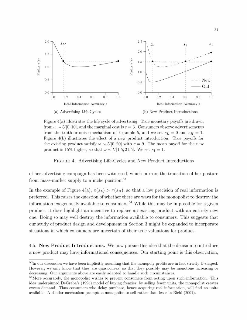
31

0.0 0.2 0.4 0.6 0.8 1.0

Real-Information Accuracy s

0.0

0.5

1.0

1.5

2.0P

rofitsπ(s

)..............................................................................................................................................................................................................................................................................................................................................................

...................................................................................................

.....................................................................••. . . . . . . . . . . . . . . . . . . . . . . . . . . .

.

.

.

.

.

.

.

.

.

.

.

.

.

.

.

.

.

.

.

.

.

.

.

sM

(a) Advertising Life-Cycles

0.0 0.2 0.4 0.6 0.8 1.0

Real-Information Accuracy s

0.0

0.5

1.0

1.5

2.0

2.5

Pro

fitsπ(s

)

.........................................................................................................................................................

................................................

..............................................

.............................................

............................................

............................................

............................................

............................................

............. . . . . . . . . . . . . . . . . . . . . . . . . . . . . . . . .•• •

.

.

.

.

.

.

.

.

.

.

.

.

.

.

.

.

.

.

.

.

.

.

.

.

.

.

.

.

.

.

.

.

.

.

.

.

.

.

.

.

.

.

.

.

.

.

.

.

.

.

.

.

.

.

.

.

.

.

.

.

.

.

.

.

.

.

.

.

.

s2 s2 s1..............................................................................

............. ............. ............. ............. ............. ............. ............. ............. ..........................

..........................

..........................

.............•

.......................................................

............. ............. .....

OldNew

(b) New Product Introductions

Figure 4(a) illustrates the life cycle of advertising. True monetary payoffs are drawnfrom ω ∼ U [0, 10], and the marginal cost is c = 3. Consumers observe advertisementsfrom the truth-or-noise mechanism of Example 5, and we set sL = 0 and sH = 1.Figure 4(b) illustrates the effect of a new product introduction. True payoffs forthe existing product satisfy ω ∼ U [0, 20] with c = 9. The mean payoff for the newproduct is 15% higher, so that ω ∼ U [1.5, 21.5]. We set s1 = 1.

Figure 4. Advertising Life-Cycles and New Product Introductions

of her advertising campaign has been witnessed, which mirrors the transition of her posture

from mass-market supply to a niche position.53

In the example of Figure 4(a), π(sL) > π(sH), so that a low precision of real information is

preferred. This raises the question of whether there are ways for the monopolist to destroy the

information exogenously available to consumers.54 While this may be impossible for a given

product, it does highlight an incentive to replace an existing product with an entirely new

one. Doing so may well destroy the information available to consumers. This suggests that

our study of product design and development in Section 3 might be expanded to incorporate

situations in which consumers are uncertain of their true valuations for product.

4.5. New Product Introductions. We now pursue this idea that the decision to introduce

a new product may have informational consequences. Our starting point is this observation,

53In our discussion we have been implicitly assuming that the monopoly profits are in fact strictly U-shaped.However, we only know that they are quasiconvex, so that they possibly may be monotone increasing ordecreasing. Our arguments above are easily adapted to handle such circumstances.54More accurately, the monopolist wishes to prevent consumers from acting upon such information. Thisidea underpinned DeGraba’s (1995) model of buying frenzies; by selling fewer units, the monopolist createsexcess demand. Thus consumers who delay purchase, hence acquiring real information, will find no unitsavailable. A similar mechanism prompts a monopolist to sell rather than lease in Biehl (2001).

32

and also the observation that firms frequently are faced with the decision of whether to con-

tinue selling an existing product or to replace it with one of improved quality. By improved

quality we mean that, fixing the precision of information available, the demand curve associ-

ated with the new product is an outward shift of that associated with the existing product.

We fix the number of consumers who will be aware of the existence of either product, and

suppose that the real information available to consumers related to the current product is

fixed at s1. The only way the monopolist can influence the information available to con-

sumers is by introducing a new product in place of the existing one. If the new product is

introduced, consumers have some stock of information s2 < s1 so that, as explained above,

introducing a new product leads to the destruction of some information.55

When will the monopolist replace her existing product with a new one? To answer this,

we observe that the change in profits can be decomposed into two effects. The first is an

increase in profits resulting from improved quality, given the original precision of information

s1, while the second is a change (either positive or negative) resulting from the fall in the

precision from s1 to s2, at the new quality level. Figure 4(b) illustrates a particular example.

Therefore, assuming that the profit function for each product is quasi-convex in s (as it

would be in a variety of circumstances as shown earlier), the monopolist faces the greatest

informational cost (if indeed there is a cost, since the monopolist may wish to destroy

information) when s1 is large, fixing s2. Heuristically, the monopolist is hurt the most by

the depletion of the informational stock because profits are highest at the extremes sL and

sH . If we associate larger values of s1 with firms that have established a meaningful brand

image that conveys important information to potential consumers, we conclude that firms

with such images will be more hesitant to innovate if so doing threatens their brand image.

Thus, the presence of these informational costs means the monopolist may not introduce a

new product even though it raises consumers’ true payoffs.

We might also ask how the new information level s2 influences new product introduction,

this time taking s1 as given. Heuristically we see that when s2 is at either a high or a low

extreme, a firm is more likely to introduce a new product. That is, if s2 is quite high (s2 > s2

in Figure 4(b)) then there is no real informational cost and the firm should proceed with

the product of higher quality. Similarly, if s2 is very low (s2 < s2), then while significant

information is destroyed, s2 is at least close to the lower extreme sL, and the monopolist will

tend to favor a new product. For more moderate information destruction (s2 < s2 < s2),

however, the response to product-innovation opportunities will be sluggish.

55In reality, there may be significant R&D costs of developing a new product, and new products may havedifferent cost structures associated with production. However, to focus on the role played by informationloss, we assume that there is no cost to innovation, and no change in the marginal production cost.

33

This discussion suggests that when these informational issues are significant the monopolist

would benefit from taking steps to either curb or enhance the destruction of information

associated with a new product’s introduction. In reality, such steps are available. One

manner in which a firm may preserve information is by designing new products to share

similar features as old products, and by promoting the new product in such a way that

consumers are aware of this. Thus the monopolist might specialize in certain styles of

products, and emphasize the similarities between them by using the same brand names for

different products developed over time.56 On the other hand, when destroying information is

beneficial, the monopolist will wish to perform extensive style changes and emphasize such

changes by, for example, using different product or brand names. Finally, we note that when

s2 is controlled by the monopolist, then she will always innovate.

5. Product Lines

In Section 2, the monopolist sold only a single product. Here we analyze a multiproduct mo-

nopolist, selling a range of quality-differentiated goods, and explore the relationship between

her product line and the dispersion of the consumer-type distribution.

The section is organized as follows. We first construct a standard model of quality-based

price-discrimination, following Mussa and Rosen (1978). Rather than employing the contract-

theoretic analysis of Maskin and Riley (1984), we use Johnson and Myatt’s (2003b, 2003a)

“upgrades approach” to obtain our results. This approach re-casts multiproduct supply de-

cisions so that one works not with the actual physical products, but instead in terms of

upgrades from one quality to the next. As we show just below, the product line may be

characterized by the usual “MR = MC” first-order condition of a single-product monopolist.

Applying this technique, we ask how the monopolist’s price-discrimination opportunities and

technological capability influence her desire to choose mass-market versus niche positions.

We then characterize the transformation of the product line following an increase in the

dispersion of consumers, before reviewing an example that illustrates our results.

5.1. The Upgrades Approach to Product Line Design. The monopolist is able to offer

n distinct product qualities, where the quality of product i is qi, and 0 < q1 < · · · < qn.

A consumer’s type θ is her willingness-to-pay for a single unit of quality. Thus, if a type θ

consumes quality q at price p, he receives a net payoff of θq − p. Faced with a set of prices

56The automobile manufacturer Jaguar recently introduced a new XJ-series luxury sedan. The engineeringof the new XJ is advanced in that it makes extensive use of lightweight construction materials; however,its styling closely resembles the XJ sedan of 30 years earlier. In a newspaper review article, Frankel (2003)commented that, “Cautiously styled to resemble an expanded version of the old XJ, it appears too keen notto offend those who have made sure Jaguar has sold more XJs over 35 years than every other model puttogether . . . [but] contrary to appearances, the XJ is the most radical big saloon on the market.”

34

{pi}, a consumer purchases a single unit of the product that maximizes θqi−pi, unless doing

so yields a negative payoff, in which case he purchases nothing.

The monopolist sets quantities for each of her n products. As in Section 2, we write P (z) for

the type θ with a mass z of others above him. This corresponds to the inverse demand curve

for a single product of quality q = 1, and is the basis for the entire system of inverse demand.

We write {zi} for the supplies of the n qualities. For the market to clear, the individual with∑nj=1 zj others above him must be just indifferent between purchasing quality q1 and not

purchasing at all. We define the cumulative variables {Zi} to satisfy Zi =∑n

j=i zj. With

this notation, p1 = q1P (Z1). Thus, the consumer of type θ = P (Z1) is just willing to buy

product 1. Similarly, a consumer with Zi others above him must be just indifferent between

products i and i− 1, so that pi − pi−1 = P (Zi)(qi − qi−1). Writing p0 = q0 = 0,

∆pi = P (Zi)∆qi for all i ∈ {1, . . . , n}.

Following Johnson and Myatt (2003b, 2003a), we offer the following interpretation. ∆pirepresents the price of an “upgrade” from quality qi−1 to the next quality qi. Thus, we can

view the monopolist as supplying Z1 units of a “baseline” product of quality q1, at a price

of p1. She then supplies successive upgrades to this baseline product in order to achieve

qualities above this. So, a product of quality q2 consists of a baseline product at a price of

p1, bundled together with an upgrade ∆q2 priced at ∆p2. Similarly, a product of quality q3consists of quality q2 bundled together with an upgrade ∆q3 priced at ∆p3.

On the cost side, the monopolist manufactures quality qi at a constant marginal cost of

ci. The profit of the monopolist can be determined given that she has chosen a profile of

upgrade supplies {Zi}, where Zi ≥ Zi+1 is required for this profile to be feasible (since

zi = Zi − Zi−1 ≥ 0). In particular, π =∑n

i=1 Zi(∆pi −∆ci), which is the same as

π =n∑i=1

πi where πi = Zi [P (Zi)∆qi −∆ci] = ∆qi × Zi

[P (Zi)−

∆ci∆qi

].

We impose two simplifying conditions.57 First, quality-adjusted marginal revenue MRs(z) =

Ps(z) + zP ′s(z) is decreasing in z for all s. Second, there are decreasing returns to quality:

∆cn∆qn

>∆cn−1

∆qn−1

> · · · > ∆c2∆q2

>∆c1∆q2

> 0.

This holds, for instance, whenever ci = c(qi) and c(q) is convex in q. Here, the primary

effect of this assumption is that it implies that a monopolist will not offer a product line

that exhibits “gaps.” That is, if products i and k > i are optimally in positive supply then

so is any product j with i ≤ j ≤ k. We can see this by examining the unconstrained supply

57Neither of these conditions is required for Proposition 9 to hold.

35

Z∗i that maximizes profits in upgrade market i, or

Z∗i = arg max

Zi∈[0,1]

∆qi × Zi

[P (Zi)−

∆ci∆qi

].

Since marginal revenue is decreasing, we can employ the usual first-order condition, equating

marginal cost to marginal revenue where possible, to characterize Z∗i . In fact,

MR(Z∗i ) = P (Z∗

i ) + Z∗i P

′(Z∗i ) =

∆ci∆qi

,

so long as marginal revenue crosses ∆ci/∆qi; otherwise the optimal (unconstrained) upgrade

output in market i is either zero or one. Now, given this, and the fact that the right-hand

side is strictly increasing in i, Z∗i must be decreasing. It is strictly decreasing whenever we

have an interior solution: Z∗i ∈ (0, 1) implies Z∗

i > Z∗i+1. Since the monotonicity constraint

Zi ≥ Zi+1 on upgrade supplies is satisfied, the set of upgrade supplies that maximize profits in

each upgrade market independently also solves the monopolist’s multiproduct maximization

problem incorporating the appropriate monotonicity constraints. Moreover, as claimed, there

clearly can be no gaps in the product line of the firm.

Note that, when an interior solution maximizes πi, the equalization of marginal revenue

and (quality-adjusted) marginal cost in the upgrade market reveals the simple economics

of second-degree price discrimination: It corresponds to the usual monopoly solution in the

space of upgrade supplies, rather than the supplies of the products themselves.

5.2. Product Lines and Distribution Families. Consider a family of type distributions

{Fs(θ)}, with associated inverse-demand functions {Ps(z)}. Exactly as above,

π(s) = max{Zis} :Zis≤Z(i−1)s ∀i

{n∑i=1

πi

}where πi = ∆qi × Zis

[Ps(Zis)−

∆ci∆qi

].

We let Z∗is denote the optimal level of upgrade i given s.

From our work in Section 2 we know that the profits of a monopolist selling a single product

are either quasi-convex or convex in s. Similar results hold for a multiproduct monopolist.58

Proposition 9. If Ps(z) is a convex function of s for each z ∈ [0, 1], then the profits π(s)

of a multiproduct monopolist are convex in s, and maxs∈S π(s) ∈ {π(sL), π(sH)}. Hence, if

the family of distributions {Fs(θ)} is ordered by a sequence of local mean-variance shifts, so

that Fs(θ) = F ((θ − µ(s))/s), and the mean µ(s) is convex, then π(s) is convex.

58As stated previously, Proposition 9 does not require either the assumption of decreasing marginal-revenueor that of decreasing returns to quality assumed earlier in this section. These two assumptions ensure thatthe constraints Zis ≥ Z(i+11)s may be neglected. Johnson and Myatt (2003b) exploited failures of these twoassumptions to explain the phenomena of “fighting brands” and “product-line pruning.”

36

The intuition behind Proposition 9 is somewhat more complicated than when there is but a

single product. To better understand it, note that we may divide the monopolist’s upgrades

into two subsets for any fixed s. For discussion purposes, we specialize to the case of mean-

variance shifts, and recall that z†s is the quantity around which the (now quality-normalized)

inverse-demand rotates for a local change in s. Suppose that, for some i,

∆ci∆qi

> MRs(z†s) >

∆ci−1

∆qi−1

⇒ Z∗is < z†s < Z∗

(i−1)s.

Hence, for all upgrades j ≥ i, optimal supply is below the rotation quantity z†s, and for all

upgrades j < i supply is above z†s. Profits are the sum of two components:

π(s) =∑j<i

∆qj × Z∗js

[Ps(Z

∗js)−

∆cj∆qj

]︸ ︷︷ ︸

Mass-Market Upgrades

+∑j≥i

∆qj × Z∗js

[Ps(Z

∗js)−

∆cj∆qj

]︸ ︷︷ ︸

Niche Upgrades

.

The “mass-market upgrades,” which include the baseline product q1, have optimal supplies

serving the mass market. A local increase in s will reduce the profitability of such upgrades.

In contrast, the supplies of “niche upgrades,” which include supply of the upgrade to the

maximum-feasible quality qn, are restricted to a niche market. The profitability of them

is increasing in s. Thus, the two sets of upgrades present a tension for the monopolist: A

mass-market posture is optimal for some, while a niche posture is optimal for the remainder.

That is, increasing s raises the profits in some upgrade markets but lowers it in others.59

It is now easy to explain why, unlike in the case of a single product (Proposition 1), quasi-

convexity of Ps(z) in s is insufficient to guarantee quasi-convexity of profits, and yet when

Ps(z) is convex in s, profits are convex in the multiproduct case just as they would be if there

were a single product. The technical reason for the distinction is that, while a multiproduct

monopolist who faces quasi-convex Ps(z) does have quasi-convex profits in each upgrade

market, there is no guarantee that the sum of the profits is quasi-convex, since the sum of

quasi-convex functions need not be quasi-convex. More heuristically, if a local increase in s

implied a slight increase in overall profits, mere quasi-convexity of πi for each i would not

ensure that a further increase does not lead to a decrease in profits, destroying quasi-convexity

of overall profits. The reason is that a further increase in s would (quite possibly) improve

the profits associated with some upgrade markets while worsening the profits associated

with others at arbitrary rates, so that more structure than quasi-convexity is required to

ensure that the positive effects of heightened s continue to outweigh the negative effects.

59This suggests that the firm would like to set different levels of s in different upgrades markets. However,each upgrade market is influenced by the same underlying distribution, and so whatever moves the demandcurve in one upgrade market moves it similarly in another.

37

The stronger condition of convexity of Ps(z) resolves this issue, and moreover leads to the

stronger conclusion that profits are convex in s.60

As noted above, if the monopolist is able to choose s, then subject to the conditions of

Proposition 9, she will select either sL or sH . Following the intuition just outlined, how-

ever, this selection will depend upon the relative importance of the niche and mass-market

upgrades. To investigate this tension further, suppose that, in fact, there are N potential

qualities available, but that the monopolist is restricted to the production of qualities qn and

below, where n < N . Suppose that, initially, ∆cn/∆qn < MRs(z†s), so that the monopolist’s

product line consists entirely of mass-market upgrades. It follows that her incentive is to

lower s. Suppose that the monopolist then innovates, and by doing so raises her technolog-

ical capabilities. We can think of this an increase in n. If ∆cN/∆qN > MRs(z†s), then for

a sufficiently large innovation, ∆cn/∆qn > MRs(z†s). The monopolist now has more niche

upgrades in her portfolio. As n increases, her profits are increasingly biased towards a niche

operation, in the sense that for a given s, the local change in profits from an increase in s

is increasing. Moreover, under some mild technical conditions, increases in s make it more

likely that the monopolist will choose sH over sL, if she is indeed able to make this choice.

Let π(s, n) denote the optimized profits given s and given that the firm can produce up to

quality qn.

Proposition 10. Suppose that the family of distributions is ordered by a sequence of mean-

variance shifts, so that Fs(θ) = F ((θ − µ(s))/s), with convex µ(s). If PsH(0) > ∆cN/∆qN ,

and n > n where MRsL(z‡sL

) < ∆cn/∆qn, then π(sH , n)−π(sL, n) is strictly increasing in n.

This says that as the monopolist becomes able to produce higher-quality products, she may

alter her strategy regarding her choice of s. As n increases, both π(sH , n) and π(sL, n)

increase, since the choice set expands, but higher levels of s become more attractive since

π(sH , n) increases more quickly than π(sL, n). Heuristically, the reason is that, under the

hypotheses above, the new upgrade will be sold as a niche upgrade for either sL or sH , and

niche upgrades are more valuable under more disperse distributions of consumer willingness-

to-pay (since marginal revenue is higher under sH than sL in the relevant range of quantity).

This line of thinking also reveals when the incentives to expend resources to so innovate are

the greatest. Intuitively, under conditions similar to those in Proposition 10, as s is higher

the incentive to invest in niche innovations is greater. Therefore, informally speaking, if

we imagine that s is increasing exogenously over time as a result increased product-design

idiosyncrasy, consumer learning about the product line, or an increase in the dispersion of

consumer wealth (and willingness-to-pay), we would expect a monopolist to accelerate her

pursuit of higher-quality products.

60Convexity of Ps(z) in s holds for the examples of Sections 2–4.

38

There are numerous further implications that follow immediately from Proposition 9. For

example, much of the discussion in Sections 2–4 for single-product firms is readily applicable

to the multiproduct setting, and we do not recapitulate here. On the other hand, the question

of how the entire product-line is influenced by changes in s is necessarily not considered in

the single-product setting, and so we turn now to that issue.

5.3. Product Line Transformations. We consider the implications of an increase in s,

which would follow from an exogenous or endogenous increase in the dispersion of consumer

valuations for quality, on the characteristics of the monopolist’s product line. To sharpen

our analysis, we restrict to a family of distribution functions {Fs(θ)} that are ordered by

a sequence of mean-variance shifts (Definition 2). From Proposition 2, we know that a

local change in s will result in a rotation of the (quality-normalized) marginal revenue term

MRs(z) = Ps(z) + zP ′s(z) around z‡s. Thus, for an upgrade i satisfying ∆ci/∆qi > MR‡

s =

MRs(z‡s), so that Z∗

is < z‡s, marginal revenue is increasing in s, and hence so is Z∗is. If the

reverse inequality holds, then Z∗is is decreasing in s. Summarizing,(

MR‡s −

∆ci∆qi

)∂Z∗

is

∂s< 0 for all i such that MR‡

s 6=∆ci∆qi

.

For instance, suppose that there is some i such that

∆ci−1

∆qi−1

< MR‡s <

∆ci∆qi

.

The supply of upgrades j ≥ i increases with s, and the supply of upgrades j < i decreases

with s. We can relate this observation back to consider the distribution of qualities offered

by a firm. Recall that Z∗js is the total supply of all qualities qj and greater. Hence, setting

Z0 = 1 for convenience for all s, 1 − Z∗js is the supply of qualities strictly below i. Thus,

{1−Z∗js} may be used to characterize the distribution of qualities offered by the monopolist.

Since 1 − Z∗js is increasing in s, for j < i, and increasing for j > i, we observe that the

cumulative distribution function of qualities supplied rotates as s increases. This argument

leads to the following proposition, which also describes further possibilities.61

Proposition 11. Suppose that the family of distributions is ordered by a sequence of mean-

variance shifts, so that Fs(θ) = F ((θ − µ(s))/s), and that µ(s) is convex. Then,

(1) if MRs(z‡s) ∈ (∆c1/∆q1,∆cn/∆qn), then a local increase in s yields a local rotation

of the distribution of qualities offered by the monopolist,

(2) if MRs(z‡s) < ∆c1/∆q1 then a local increase in s yields a first-order stochastic domi-

nating shift up in the distribution of qualities offered by the monopolist, and

61The three responses of the product line to s, as described in Proposition 11, fall within Hammond’s (1974)notion of “simply related” distributions. Thus, if a local change in s results in two distributions of θ thatare simply related, then the corresponding distributions of qualities supplied will also be simply related.

39

(3) if MRs(z‡s) > ∆cn/∆qn then a local increase in s yields a first-order stochastic dom-

inated shift down in the distribution of qualities offered by the monopolist.

As marginal revenue rotates, more upgrades are produced of those qualities with (quality-

adjusted) marginal production costs above the rotation point of (quality-adjusted) marginal

revenue, while fewer upgrades of other qualities are produced. When MRs(z‡s) < ∆c1/∆q1,

in the region of relevance marginal revenue is rising for each given upgrade quality and

consequently Z∗is is increasing for each i: For each given quality level, the total number of

products of at least that quality increases. An implication is that more products in total are

on the market. On the other hand, when MRs(z‡s) > ∆cn/∆qn, in the region of relevance

marginal revenue is falling for each given upgrade quantity and consequently Z∗is is decreasing

for each i: For each given quality level, the total number of products of at least that quality

decreases. An implication of this is that fewer products in total are on the market. For the

remaining case (statement (1) in the proposition) the total output produced at or above a

particular quality level goes up or down, depending on the quality level in question.

Finally, it is important to note that in none of these cases can we typically make direct

conclusions about the output of any particular quality itself. Instead, we predict changes in

the overall volume either above or below certain quality levels. That is, we predict changes in

the levels of the upgrades, but without additional structure one cannot say how the difference

in upgrade levels z∗is = Z∗is − Z∗

(i+1)s (the supply of the actual product i) will change with

s. The reason is that this depends on the relative slopes of marginal revenue at different

quality-normalized cost levels, and these slopes are in no way tied down by the assumptions

we have made. An exception is the highest quality product that is in positive supply. For

this product i the supply of the complete product z∗is is equal to the supply Z∗is of upgrade

i, since Z∗(i+1)s = 0. z∗is is then locally increasing or decreasing in s depending upon whether

∆ci/∆qi is above or below MR‡s.

We now examine the boundaries of the monopolist’s product line. Intuitively, we expect

predictable changes to the lower and upper product ranges. In particular, we expect the

monopolist to expand the set of qualities offered as s increases. To investigate this, we write

qs

and qs for the lowest and highest qualities offered.

Proposition 12. Suppose that the family of distributions is ordered by a sequence of mean-

variance shifts, so that Fs(θ) = F ((θ − µ(s))/s), and that µ(s) is convex. Then the monop-

olist’s product range expands with s: qs

is decreasing and qs is increasing.

One implication of this proposition is that a long product line complements actions that

increase the dispersion of consumer willingness-to-pay. Moreover, extending the product line

both on the low and the high quality ends may well accompany such increased dispersion. One

concrete application is the evolution of a product line over time. If s represents information

40

0.00 0.75 1.50 2.25

Quality q

0.0

0.2

0.4

0.6

0.8

1.0D

istr

ibuti

on

Funct

ionG

s(q

)

•

.......................................................

............. ............. .....

. . . . .

s = 0.8

s = 0.5

s = 0.2•.................................................................................

.................................

...................................

...................................

.....................................

......................................

.........................................

.........................................

...........................................

.............................................

........................................•

•.....................................................................................................................

..........................

..........................

..........................

..........................•

•.................................•

(a) Rotated Distributions of Quality

0.00 0.75 1.50 2.25

Quality q

0.0

0.3

0.6

0.9

1.2

Den

sity

Funct

iong

s(q

)

..............................................................................................................................................................................................................................................................................................................................................................................................................................................................................................................................................................................................................•

.............

.............

..............................................................................

............. ............. ............. ............. ............. ............. ............. ............. ............. ............. ............. .....•

•. ...... . . . . . . . . . . .•

(b) Stretched Densities of Quality

These figures illustrate the change in the monopolist’s product line in response to s,following the specification of Example 7. The parameters are γ = µ = 1 and α = 3

4 .

Figure 5. Changing Product Lines from Example 7

about product characteristics, and if the overall market becomes better informed over time,

the optimal strategy for a monopolist will be to begin with a focused product line, but to

then expand it in both directions as information accumulates in the market.

Putting Propositions 11 and 12 together, we see that while the monopolist’s product line

always expands with s, whether this expanded range results in a larger or smaller total

supply depends on the rotation point of marginal revenue. For example, suppose that the

marginal cost of the baseline product is relatively low, so that MR‡s = MRs(z

‡s) > c1/q1. This

implies that Z∗1s is locally decreasing in s. Thus, as the dispersion of types increases, the

monopolist will serve less of the total market. However, she will do so using more products.

5.4. Illustration. To illustrate our results, we expand the single-product setting of Exam-

ple 1 to include the possibility of a quality-differentiated multiproduct menu.

Example 7. Consumer types follow the specification of Example 1. The monopolist may

produce any quality q ∈ [0, q]. If she is able to manufacture quality q, then the monopolist

may do so by paying a constant marginal cost of c(q) = γq1+α/(1 + α), where α, γ > 0.

Example 7 does not describe a discrete grid of available qualities, but instead allows the

monopolist to choose from a continuum. Nevertheless, we may apply our analysis by spec-

ifying a grid of n qualities satisfying qn = q and q0 = 0. For ∆qi sufficiently small, the

quality-normalized marginal cost of upgrade i satisfies ∆ci/∆qi ≈ c′(qi) = γqαi . Employing

41

Proposition 3, for an interior solution Z∗is ∈ (0, 1), the supply of upgrade i satisfies

Z∗is =

1

4s

[s+ µ− ∆ci

∆qi

]≈ s+ µ− γqαi

4s.

Allowing n to grow large, we may consider the limiting case in which the monopolist sells

a continuum of qualities. Omitting the details of this limiting operation, we write Gs(q) for

the distribution function over qualities for given s, and gs(q) for its corresponding density:

Gs(q) = 1− s+ µ− γqα

4sand gs(q) =

γαqα−1

4s.

It is also straightforward to obtain the upper and lower bounds to the product line:

qs=

[max{0, µ− 3s}

γ

]1/α

and qs = min

{[µ+ s

γ

]1/α

, q

},

where the monopolist does in fact operate so long as µ + s > 0. For q sufficiently large

(so that the monopolist is able to manufacture products of very high quality) the optimal

product lines are illustrated in Figure 5, for varying s. For lower s (for instance, s = 0.2) the

lower bound of the product line is strictly above zero. As s increases, however, the upper

and lower bounds to the product line move up and down, respectively, until the lower bound

hits q = 0. Further increases in s prompt the monopolist to restrict her total output—as

noted previously, she sells fewer units in total, but uses a longer product-line to do so.

6. Concluding Remarks

We have proposed a framework for analyzing both exogenous and endogenous transforma-

tions of the demand facing a firm. Our approach is based on the observation that changes in

demand frequently correspond to changes in the dispersion of the underlying willingness-to-

pay of consumers, which lead to a rotation of the demand curve. We investigated numerous

applications of our framework, including product design and development decisions, adver-

tising and marketing activities, and product line choices of multiproduct firms. The optimal

advertising and product design depend, in turn, on the monopolist’s desire to adopt either

a mass-market or niche posture. We also suggested a new taxonomy of advertising, distin-

guishing between hype, which shifts demand, and real information, which rotates demand.

It has not escaped our attention that there are limitations to our analysis. Perhaps most

importantly, we have considered only a single firm. Introducing more firms may engender

strategic interactions, modifying our results and generating new ones. Nonetheless, because

demand dispersion possibilities influence a multitude of choices that a firm makes, better

understanding their role seems critical to a fuller appreciation of firm-level decision making.

The steps taken here by us will be helpful in this regard. One reason is that there has been

remarkably little prior study of this issue. A more important reason may be that, while

42

our framework is broadly applicable, it is also very simple: Understanding the economics of

demand rotations suffices to understand many phenomena from diverse areas of application.

Appendix A. Omitted Proofs

Propositions 1, 5, 7, 9, and 11 follow from arguments presented in the main text.

Proof of Lemma 1. Fix θ and s′, s′′ ∈ S, where s′ < s′′. If statement (1) holds, then

∂Fs′(θ)

∂s≤ 0 ⇒ θ ≥ θ†s′ ≥ θ†s′′ ⇒ ∂Fs′′(θ)

∂s≤ 0.

Thus, if Fs(θ) is weakly decreasing in s, then it also weakly decreasing for larger s. Equiva-

lently, Fs(θ) is quasi-concave in s; this is statement (3). If statement (1) does not hold then

we may find s′ < s′′ such that θ†s′ < θ†s′′ . Fixing θ satisfying θ†s′ < θ < θ†s′′ ,

∂Fs′(θ)

∂s< 0 <

∂Fs′′(θ)

∂s.

This means that Fs(θ) is first decreasing, and then increasing, as s increases; it is not quasi-

concave, and statement (3) must fail. Combining these observations, we have shown that

statement (1) holds if and only if statement (3) holds. Very similar arguments confirm that

these are also equivalent to statements (2) and (4). �

Proof of Propostion 2. Profits satisfy π(s) = maxz∈[0,1]{zPs(z)−C(z)}. Since Ps(z) = µ(s)+

sP (z), and µ(s) is convex, Ps(z) is the sum of convex functions and hence convex in s, as

is zPs(z) − C(z). π(s) is then the maximum of convex functions, and is itself convex. We

turn to statements (1)–(4). For a given z, the derivative of marginal revenue with respect

to s is µ′(s) + P (z) + zP ′(z). Decreasing marginal-revenue immediately reveals that there

is some z‡s ∈ [0, 1] such that this derivative is positive if z < z‡s, and negative if z > z‡s. This

represents a local rotation, establishing statement (1).62 By inspection, marginal revenue

is convex in s, yielding statement (2). The first part of statement (3), claiming that z‡s is

increasing in s, and statement (4), follow from the logic used in the proof of Lemma 1. The

second part of statement (3), claiming that z‡s < z†s, follows from the observation that

0 =∂MRs(z

‡s)

∂s= µ′(s) + P (z‡s) + z‡sP

′(z‡s) < µ′(s) + P (z‡s) =∂Ps(z

‡s)

∂s⇒ z‡s < z†s.

Statements (1)–(4) also imply quasi-convexity of z∗s in s. Note that MRs(z∗s) = C ′(z∗s). If z∗s

is locally increasing in s, then marginal revenue, evaluated at z∗s , must also be increasing:

z∗s < z‡s. z‡s is increasing. It follows that, for any z < z∗s and any larger s′ > s it must be the

case that MRs′(z) > C ′(z). This ensures that z∗s must continue to increase with s.

62The notion of a rotation (Definition 1) must be modified slightly to allow for rotation quantities of z‡s = 1and z‡s = 0. For these cases the marginal revenue curve shifts up (z‡s = 1) or down (z‡s = 0) with s.

43

Finally, statements (5)–(8). MR‡s is decreasing in s. Hence, if c > MR‡

sL, then c > MR‡

s for

all s. It follows that z∗s < z‡s, and hence z∗s must be increasing for all s, yielding statement

(5). Statements (6) and (7) follow in a similar fashion. Statement (8) refers to case in which

s indexes a sequence of mean-preserving rotations. Observe that θ†s = µ and that

MRs(z) = µ+ s[P (z) + zP ′(z)] ⇒ ∂MRs(z‡s)

∂s= P (z‡s) + z‡sP

′(z‡s) = 0,

so that MR‡s = µ is invariant to s, ensuring that z∗s is monotonic. �

Proof of Proposition 3. Given Ps(z) = µ+s(1−2z), the monopolist’s profits from the supply

of z units are z[µ − c + s(1 − 2z)]. The first-order condition for an interior solution yields

z∗s = (s + µ − c)/4s and profits of π(s) = (s + µ − c)2/8s, as stated. Minimization of π(s)

yields s = µ− c. When 0 ≤ s ≤ c−µ or 0 ≤ 3s ≤ µ− c then we obtain a boundary solution

z∗s ∈ {0, 1}. Simple algebra yields the remaining elements of statements (1)–(3). Statement

(4) is obtained by solving π(sH) = π(sL) for sH in terms of sL. �

Proof of Proposition 4. To apply Lemma 1, we need µ′(s)/σ′(s) to be weakly increasing,

which is equivalent to the inequality µ′′(s)σ′(s) ≥ µ′(s)σ′′(s). For s ∈ [0, 1], the standard

deviation of valuations satisfies σ(s) =√σ2 + sκ2. Hence

σ′(s) =κ2

2√σ2 + sκ2

⇒ σ′′(s)

σ′(s)= − κ2

2(σ2 + sκ2)= − 1

2([σ2/κ2] + s),

which upon substitution yields the desired inequality. �

Proof of Lemma 2. Under the specification of the lemma, and setting µ = 0 without loss of

generality, the inverse-demand curve faced by the monopolist satisfies

Ps(z) = exp

(−s

2

2+ sH(z)

)where H(z) = Φ−1(1− z),

⇒ MRs(z) = Ps(z)[1 + szH ′(z)] = exp

(−s

2

2+ sΦ−1(1− z)

)×

[1− sz

φ(Φ−1(1− z))

],

where Φ(·) is the distribution function of the standard normal, and φ(·) is the density.

MRs(z) is decreasing in z wherever it is positive. To see this, write x = Φ−1(1− z), so that

z = 1− Φ(x) ⇒ MRs(z) = exp

(−s

2

2+ sx

)×

[1− s[1− Φ(x)]

φ(x)

]⇒ ∂MRs(z)

∂z= − s

φ(x)

[MRs(z)− exp

(−s

2

2+ sx

)∂

∂x

(1− Φ(x)

φ(x)

)].

The hazard rate φ(x)/(1−Φ(x)) is increasing in x; it follows that the bracketed term in the

expression above is positive whenever MRs(z) ≥ 0. Since marginal revenue is decreasing, this

means that MRs(z†s) > c implies that z∗s > z†s; similarly MRs(z

†s) < c implies that z∗s < z†s.

44

For the evaluation of MRs(z†s), differentiating Ps(z) with respect to s yields ∂Ps(z)/∂s =

0 ⇔ s = H(z), so that s = Φ−1(1− z†s), or equivalently z†s = 1− Φ(s). Evaluated at z†s,

MR†s = MRs(z

†s) = exp

(s2

2

)×

[1− s[1− Φ(s)]

φ(s)

].

For intersections of z†s and z∗s , recall that if z†s 6= z∗s then (z∗s − z†s)(MR†s − c) > 0. Hence,

to show that z∗s crosses z†s at most once, and from above, MR†s must cut c once, and from

above. Hence, a sufficient condition for quasi-convexity of profits it that MR†s is decreasing:

dMR†s

ds= exp

(s2

2

)×

[2sφ(s)− (1 + 2s2)[1− Φ(s)]

φ(s)

]< 0 ⇔ φ(s)

1− Φ(s)< s+

1

2s,

where in calculating the derivative we exploited the fact that ∂φ(s)/∂s = −sφ(s). This last

inequality reduces to s < s ≈ 0.925, where s is the unique solution to φ(s)/(1 − Φ(s)) =

s + (1/2s); we obtained this solution via a numerical study of this equation. A similar

argument ensures that MR†s is increasing for s > s, and hence monopoly profits are quasi-

concave in this second region. �

Proof of Proposition 6. The argument given in the text ensures that the monopolist will wish

to choose κ ∈ {κL, κH}. For the second claim, notice that π(sH)− π(sL) = π(√σ2 + κ2

H)−π(

√σ2 + κ2

L) is increasing in σ. If π(κH) > π(κL), then we set σ = 0, and the claim holds. If

not, then we observe that π(√σ2 + κ2

H) > π(√σ2 + κ2

L) for σ sufficiently large. This follows

from the observation that, if σ is sufficiently large, then z∗ < 1/2. �

Proof of Proposition 8. A consumer updates his prior ω ∼ N(µ, κ2) following the observation

of the signal x |ω ∼ N(ω, ξ2). Standard calculations confirm that his posterior satisfies

ω |x ∼ N

(κ2x+ ξ2µ

κ2 + ξ2,κ2ξ2

κ2 + ξ2

)or equivalently N

(µ+ ψκ2x

1 + ψκ2,

κ2

1 + ψκ2

).

Given CARA preferences, and the normality of posterior beliefs over ω, the consumer’s

willingness to pay will be the certainty equivalent E[ω |x]−λ var[ω |x]/2. Substituting in for

the expectation and variance yields the expression for θ(x) given in the main text. With such

preliminaries in hand, we may turn to the proposition itself. In a slight abuse of notation,

let us write σ2 for the variance of θ. Following some algebraic manipulation,

Pκ2,ψ(z) = µ− λκ2

2+λs2

2+ σP (z) where s =

√ψκ4

1 + ψκ2.

Let us fix κ2. By inspection Pκ2,ψ(z) is convex in s, and s in turn is increasing in ψ. Thus

Pκ2,ψ(z) is quasi-convex in ψ. Hence profits are quasi-convex in ψ. Furthermore,

∂Pκ2,ψ(z†s)

∂ψ= 0 ⇔ λs = −P (z†ψ) ⇔ z†ψ = Φ(λs),

45

which, upon substitution of s, yields z†ψ in Footnote 47. Next, let us fix ψ. Differentiating,

∂Pκ2,ψ(z)

∂κ2= −λ

2+ [λs+ P (z)]

∂s

∂κ2= 0 ⇔ z = z†κ2 = Φ

(− λ

2(∂s/∂κ2)+ λs

).

To assess the quasi-convexity of profits in κ2, we apply Proposition 1. Examining z†κ2 ,

∂z†κ2

∂κ2≥ 0 ⇔ λ

2(∂s/∂κ2)2

∂2s

∂(κ2)2+ λ

∂s

∂κ2≥ 0 ⇔ 2

[∂s

∂κ2

]3

+∂2s

∂(κ2)2≥ 0.

To verify this last inequality, differentiate s with respect to κ2 to obtain

∂s

∂κ2=

(2 + ψκ2)√ψ

2(1 + ψκ2)3/2and

∂2s

∂(κ2)2= −(4 + ψκ2)ψ3/2

4(1 + ψκ2)5/2.

The desired inequality becomes

(2 + ψκ2)3ψ3/2

4(1 + ψκ2)9/2≥ (4 + ψκ2)ψ3/2

4(1 + ψκ2)5/2⇔ (2 + ψκ2)3 ≥ (4 + ψκ2)(1 + ψκ2)2 ⇔ 4 ≥ 0,

which establishes the claimed quasi-convexity of profits. Next, we observe that

∂Pκ2,ψ(z)

∂κ2= −λ

2+∂Pκ2,ψ(z)

∂ψ× ∂s/∂κ2

∂s/∂ψ.

Inspection of this expression yields the remaining claims of the Proposition. �

Proof of Proposition 10. Take n > n, and consider increasing n to n + 1. Considering the

profits under sL and under sH , we know that the change in either profit level is determined

solely by any additional profits gained from upgrade n + 1, because our assumptions of

decreasing marginal-revenue and decreasing returns to quality ensure that the monotonicity

constraints Zi ≥ Zi+1 can be ignored for interior upgrade supplies, as explained in the text.

Since MRsL(z‡sL

) < ∆cn/∆qn < ∆cn+1/∆qn+1, we know that Z∗(n+1)sL

< z‡sL. While it need

not be the case that MRsH(z) is a rotation of MRsL

(z), we do know that MRsH(z) > MRsL

(z)

for all z < Z∗(n+1)sL

. (See the comment given in footnote 10 on page 8 of the text.) We

conclude that Z∗(n+1)sH

≥ Z∗(n+1)sL

. Since PsH(0) > ∆cN/∆qN ≥ ∆cn+1/∆qn+1, we also

know that Z∗(n+1)sH

is strictly positive. Together, these facts plus the observation that the

true marginal-revenue associated with upgrade i is ∆qn+1MRs(z) imply that the additional

profits available in upgrade market n+ 1 are higher under sH than sL. �

Proof of Proposition 12. Fix s and consider the set of unconstrained upgrade supplies {Z∗is}

that maximize profits in each of the upgrade markets. To prove the desired result, it is

to sufficient to show that no product that is in positive supply for some s is set to zero

supply as s rises. Suppose Z∗is > Z∗

(i+1)s, so that the complete product i is in positive supply.

If for some higher s′, product i is not being supplied, then either Z∗is′ = Z∗

(i+1)s′ = 1 or

Z∗is′ = Z∗

(i+1)s′ = 0, where we can rule out interior possibilities because ∆ci/∆qi is strictly

46

increasing and marginal revenue is decreasing, as discussed in the text. Now, it cannot be

that Z∗is′ = Z∗

(i+1)s′ = 1, since MRs(1) is decreasing in s, so that the fact Z∗(i+1)s < 1 implies

Z∗(i+1)s′ < 1. Also, it can’t be that Z∗

is′ = Z∗(i+1)s′ = 0, since MRs(0) = Ps(0) is increasing in

s, so that Z∗is > 0 implies that Z∗

is′ > 0. �

Proof of Claim in Footnote 21 on Page 15. To prove this claim, we set c = 0 without loss

of generality, so that π(s) = (s + µ(s))2/8s. If π(s) achieves a strictly profitable (π(s) > 0)

maximum at some interior s ∈ (sL, sH) then the first-order condition π′(s) = 0 must be

satisfied. Differentiating π(s), we obtain

π′(s) =(s+ µ(s))[2s(1 + µ′(s))− (s+ µ(s))]

8s2= 0 ⇒ s+ µ(s) ∈ {0, 2s(1 + µ′(s))}.

Since we are restricting to strictly profitable maxima, it must be the case that π(s) > 0

and hence µ(s) + s > 0. This simply says that the highest type consumer (with valuation

µ(s) + s, by definition) is willing to pay the marginal cost of production. For π′(s) = 0 to

be satisfied, it must be the case that s+ µ(s) = 2s(1 + µ′(s)). Now, since profits are locally

maximized, the second-order condition π′′(s) ≤ 0 must be satisfied:

π′′(s) =1 + 2µ′(s) + sµ′′(s) + µ(s)µ′′(s) + (µ′(s))2

4s− 2π′(s)

s≤ 0.

Evaluated at a stationary point of π(s), the final term disappears since π′(s) = 0. The

second-order condition holds if and only if the numerator of the first term is negative, or

µ′′(s) ≤ −(µ′(s))2 + 2µ′(s) + 1

s+ µ(s)= −(µ′(s) + 1)2

s+ µ(s)= −s+ µ(s)

4s2,

where the final equality follows after substituting in the first order condition. Following the

re-introduction of the marginal cost c, this is the desired expression. �

Proof of Claim in Footnote 49 on Page 29. For the counter-example to the quasi-convexity

of profits, we need to find a dispersion index [sL, sH ] such that z†s is decreasing for some s. To

do this, we begin by specifying functions κ2(s) and ψ(s) that are increasing and continuous

in s, and then set Ps(z) = Pκ2(s),ψ(s)(z). This yields a family of demand curves ordered by a

sequence of local rotations. As part of this, let us ensure that for s = s′, a local increase in s

raise ψ but not κ2. This implies z†s′ = z†ψ >12. Furthermore, we ensure that for s = s′′ > s′,

increases in s raise κ2 but not ψ. This implies that z†s′′ = z†κ2 <12. Thus, for some s ∈ (s′, s′′),

the rotation quantity z†s must fall with s. In this manner, we have constructed an example

in which the conditions of Proposition 1 do not hold. Further trickery ensures that quasi-

convexity of profits might well fail. Note also that, at the point s at which z†s is decreasing,

it must be the case that z†κ2 < z†s < z†ψ; this reveals the design-information tension. �

47

References

Ackerberg, D. A. (2001): “Empirically Distinguishing Information and Prestige Effectsof Advertising,” RAND Journal of Economics, 32(2), 316–33.

(2003): “Advertising, Learning, and Consumer Choice in Experience Good Markets:An Empirical Examination,” International Economic Review, 44(3), 1007–40.

Adams, W. J., and J. L. Yellen (1976): “Commodity Bundling and the Burden ofMonopoly,” Quarterly Journal of Economics, 90(3), 475–98.

Aislabie, C. J., and C. A. Tisdell (1988): “Profit Maximization and Marketing Strate-gies: Demand Rotation and Social Influences,” Managerial and Decision Economics, 9(1),77–82.

Anderson, S. P., and R. Renault (2002): “Advertising Content,” Working Paper.Arrow, K. J. (1970): “The Theory of Risk Aversion,” in Essays in the Theory of RiskBearing, ed. by K. J. Arrow. North Holland, Amsterdam and London.

Atkinson, A. B. (1970): “On the Measurement of Inequality,” Journal of Economic The-ory, 2(3), 244–63.

Bagwell, K. (2003): “The Economic Analysis of Advertising,” chapter for the forthcomingHandbook of Industrial Organization.

Barndorff-Nielsen, O. (1978): Information and Exponential Families. Wiley, New York.Baron, D., and R. Myerson (1982): “Regulating a Monopolist with Unknown Costs,”Econometrica, 50(4), 911–30.

Becker, G. S., and K. M. Murphy (1993): “A Simple Theory of Advertising as a Goodor Bad,” Quarterly Journal of Economics, 108(4), 942–64.

Biehl, A. R. (2001): “Durable-Goods Monopoly with Stochastic Values,” RAND Journalof Economics, 32(3), 565–77.

Blackwell, D. (1953): “Equivalent Comparisons of Experiments,” The Annals of Math-ematical Statistics, 24(2), 265–72.

Butters, G. R. (1977): “Equilibrium Distributions of Sales and Advertising Prices,” Re-view of Economic Studies, 44(3), 465–91.

Coes, D. V. (1977): “Firm Output and Changes in Uncertainty,” American EconomicReview, 67(2), 249–51.

Comanor, W. S., and T. A. Wilson (1967): “Advertising Market Structure and Perfor-mance,” Review of Economics and Statistics, 49(4), 423–40.

(1971): “On Advertising and Profitability,” Review of Economics and Statistics,53(4), 408–10.

Cremer, J., F. Khalil, and J.-C. Rochet (1998): “Contracts and Productive Informa-tion Gathering,” Games and Economic Behavior, 25(2), 174–93.

DeGraba, P. (1995): “Buying Frenzies and Seller-Induced Excess Demand,” RAND Jour-nal of Economics, 26(2), 331–42.

Diamond, P. E., and J. E. Stiglitz (1974): “Increases in Risk and Risk Aversion,”Journal of Economic Theory, 8(3), 337–60.

Dixit, A., and V. Norman (1978): “Advertising and Welfare,” Bell Journal of Economics,9(9), 1–17.

Dorfman, R., and P. O. Steiner (1954): “Optimal Advertising and Optimal Quality,”American Economic Review, 44(5), 826–36.

48

Dowling, G. R. (1980): “Information Content in US and Austrialian Television Advertis-ing,” Journal of Marketing, 44(4), 34–7.

Erdem, T., and M. P. Keane (1996): “Decision-Making Under Uncertainty: Captur-ing Dynamic Brand Choice Processes in Turbulent Consumer Goods Markets,” MarketingScience, 15(1), 1–20.

Frankel, A. (2003): “All Sweetness and Light: Review of Jaguar XJ8,” Sunday Times(London), Sunday, March 16.

Grossman, G. M., and C. Shapiro (1984): “Informative Advertising with DifferentiatedProducts,” Review of Economic Studies, 51(1), 63–81.

Grossman, S., and O. D. Hart (1983): “Implicit Contracts Under Asymmetric Informa-tion,” Quarterly Journal of Economics, 98(3), 123–56.

Hadar, J., and W. R. Russell (1969): “Rules for Ordering Uncertain Prospects,” Amer-ican Economic Review, 59(1), 25–34.

Hammond, J. S. (1974): “Simplifying the Choice Between Uncertain Prospects wherePreference is Non-Linear,” Management Science, 20(7), 1047–72.

Hanoch, G., and H. Levy (1969): “The Efficiency Analysis of Choices Involving Risk,”Review of Economic Studies, 36(3), 335–46.

Hardy, G. H., J. E. Littlewood, and G. Polya (1929): “Some Simple InequalitiesSatisfied by Convex Functions,” Messenger of Mathematics, 58, 145–52.

(1934): Inequalities. Cambridge University Press, Cambridge.Holmstrom, B. R. (1982): “Managerial Incentive Schemes—A Dynamic Perspective,” inEssays in Economics and Management in Honour of Lars Wahlbeck, pp. 209–30. SvenskaHandelshogskolan, Helsinki.

Hutton, R. (2001): “Clever Disguise: Ray Hutton Tests the New 7-Series,” Sunday Times(London), Sunday, October 21.

Jewitt, I. (1987): “Risk Aversion and the Choice Between Risky Prospects: The Preser-vation of Comparative Statics Results,” Review of Economic Studies, 54(1), 73–85.

(1989): “Choosing Between Risky Prospects: The Characterization of ComparativeStatics Results, and Location Independent Risk,” Management Science, 35(1), 60–70.

Johnson, J. P. (2003): “Entry-Level Products with Consumer Learning,” Cornell Univer-sity Working Paper.

Johnson, J. P., and D. P. Myatt (2003a): “Multiproduct Cournot Oligopoly,” OxfordUniversity Department of Economics Discussion Paper number 145.

(2003b): “Multiproduct Quality Competition: Fighting Brands and Product LinePruning,” American Economic Review, 93(3), 748–74.

Karlin, S. (1957): “Polya Type Distributions, II,” Annals of Mathematical Statistics, 28(2),281–308.

(1968): Total Positivity. Stanford University Press, Stanford, CA.Karlin, S., and F. Proschan (1960): “Polya Type Distributions of Convolutions,” An-nals of Mathematical Statistics, 31(3), 721–36.

Kihlstrom, R. E., D. Romer, and S. Williams (1981): “Risk Aversion with RandomInitial Wealth,” Econometrica, 49(4), 911–20.

Laczniak, G. R. (1979): “Information Content in Print Advertising,” Journalism Quar-terly, 56(2), 324–27.

49

Lancaster, K. J. (1966): “A New Approach to Consumer Theory,” Journal of PoliticalEconomy, 74(2), 132–157.

(1971): Consumer Demand: A New Approach. Columbia University Press, NewYork.

(1975): “Socially Optimal Product Differentiation,” American Economic Review,65(4), 567–85.

Lehmann, E. L. (1955): “Ordered Families of Distributions,” Annals of MathematicalStatistics, 26(3), 399–419.

Leland, H. E. (1972): “Theory of the Firm Facing Uncertain Demand,” American Eco-nomic Review, 62(3), 278–91.

Lewis, T. R., and D. E. M. Sappington (1991): “All-or-Nothing Information Control,”Economics Letters, 37(2), 111–13.

(1994): “Supplying Information to Facilitate Price Discrimination,” InternationalEconomic Review, 35(2), 309–27.

Machina, M. J., and J. W. Pratt (1997): “Increasing Risk: Some Direct Constructions,”Journal of Risk and Uncertainty, 14(2), 103–27.

Madden, C. S., M. J. Caballero, and S. Matsukubo (1986): “Analysis of InformationContent in US and Japanese Magazine Advertising,” Journal of Advertising, 15(3), 38–45.

Maskin, E., and J. G. Riley (1984): “Monopoly with Incomplete Information,” RANDJournal of Economics, 15(2), 171–196.

McAfee, R. P., J. McMillian, and M. D. Whinston (1989): “Multiproduct Monop-oly, Commodity Bundling, and Correlation of Values,” Quarterly Journal of Economics,104(2), 371–83.

Meyer, M. A. (1994): “The Dynamics of Learning with Team Production: Implicationsfor Task Assignment,” Quarterly Journal of Economics, 109(4), 1157—84.

Milgrom, P. R., and J. Roberts (1986): “Price and Advertising Signals of ProductQuality,” Journal of Political Economy, 94(4), 796–821.

Milgrom, P. R., and R. Weber (1982): “A Theory of Auctions and Competitive Bid-ding,” Econometrica, 50(5), 1089–1122.

Mussa, M., and S. Rosen (1978): “Monopoly and Product Quality,” Journal of EconomicTheory, 18(2), 301–317.

Nachman, D. C. (1982): “Preservation of ‘More Risk Averse’ under Expectation,” Journalof Economic Theory, 28(2), 361–8.

Nelson, P. (1974): “Advertising as Information,” Journal of Political Economy, 82(4),729–54.

(1975): “The Economic Consequences of Advertising,” Journal of Business, 48(2),213–41.

Ottaviani, M., and A. Prat (2001): “The Value of Public Information in Monopoly,”Econometrica, 69(6), 1673–83.

Persico, N. (2000): “Information Acquisition in Auctions,” Econometrica, 68(1), 135–48.Pratt, J. W. (1964): “Risk Aversion in the Small and the Large,” Econometrica, 32(1–2),122–36.

Renforth, W., and S. Raveed (1983): “Consumer Information Cues in Television Ad-vertising: A Cross Country Analysis,” Journal of the Academy of Marketing Science, 11(1),216–25.

50

Resnik, A. J., and B. L. Stern (1977): “An Analysis of Information Content in TelevisionAdvertising,” Journal of Marketing, 41(1), 50–3.

Ross, S. A. (1981): “Some Stronger Measures of Risk Aversion in the Small and the Largewith Applications,” Econometrica, 49(3), 621–38.

Rothschild, M., and J. E. Stiglitz (1970): “Increasing Risk I: A Definition,” Journalof Economic Theory, 2(3), 225–43.

(1971): “Increasing Risk II: Its Economic Consequences,” Journal of EconomicTheory, 3(1), 66–84.

Schmalensee, R. (1982): “Commodity Bundling by a Single-Product Monopolist,” Jour-nal of Law and Economics, 25(1), 67–71.

(1984): “Gaussian Demand and Commodity Bundling,” Journal of Business, 57(1),S211–30.

Schmeidler, D. (1979): “A Bibliographical Note on a Theorem of Hardy, Littlewood, andPolya,” Journal of Economic Theory, 20(1), 125–28.

Senstrup, P. (1985): “Information Content in TV Advertising: Consumer Policy Implica-tions of the Growing Supply of TV Advertising in Europe,” Journal of Consumer Policy,8(3), 239–65.

Shapiro, C. (1980): “Advertising and Welfare: Comment,” Bell Journal of Economics,12(2), 749–51.

(1982): “Consumer Information, Product Quality, and Seller Reputation,” BellJournal of Economics, 13(1), 20–35.

Sobel, J. (1993): “Information Control in the Principal-Agent Problem,” InternationalEconomic Review, 34(2), 259–69.

Stern, B. L., and A. J. Resnik (1991): “Information Content in Television Advertising:A Replication and Extension,” Journal of Advertising Research, 31(2).

Stern, B. L., A. J. Resnik, and E. L. Grubb (1977): “Information Content in Televi-sion Advertising: A Further Analysis,” in Contemporary Marketing Thought, ed. by B. A.Greenberg, and D. M. Bellenger. American Marketing Association, Chicago.

Stigler, G. J. (1961): “The Economics of Information,” Journal of Political Economy,69(3), 213–25.

(1968): “A Note on Block Booking,” in The Organization of Industry, ed. by G. J.Stigler. Richard D. Irwin, Homewood, IL.

Stigler, G. J., and G. S. Becker (1977): “De Gustibus Non Est Disputandum,” Amer-ican Economic Review, 67(2), 76–90.

Taylor, D. B. (1983): “The Information Content of Women’s Magazine Advertising in theUK,” European Journal of Marketing, 17(5), 28–32.

Weinberger, M. G., and H. E. Spotts (1989): “A Situational View of InformationContent in TV Advertising in the US and UK,” Journal of Marketing, 53(1), 89–94.

Wilkinson, S. (2002): “uDrive Me Crazy,” Popular Science, October 31.