On the Relationship between Fiscal Plans in the European Union:

An Empirical Analysis Based on Real-Time Data*

Massimo Giuliodori** University of Amsterdam and DNB

and

Roel Beetsma***

University of Amsterdam, Tinbergen Institute, CEPR and CESifo

This version: 6 December 2006

ABSTRACT

We investigate the interdependence of fiscal policies, and in particular deficits, in the European Union using an empirical analysis based on real-time fiscal data. There are many potential reasons why fiscal policies could be interdependent, such as direct externalities due to cross-border public investments, yardstick competition, tax competition and peer pressure among governments. The advantage of using real-time data is that they better reflect the policymakers’ intentions than revised data. Real-time data allow us to investigate how available information is mapped into policymakers’ plans, while revised data are generally “polluted” with ad hoc reactions to unexpected developments that have taken place after the plan was made. Controlling for a large set of relevant determinants of primary cyclically adjusted deficits, we find indeed evidence of fiscal policy interdependence. However, the interdependence is rather asymmetrically distributed: the fiscal stances of the large countries affect the fiscal stances of the small countries, but not vice versa. Keywords: Fiscal policy interdependence, real-time data, European Union, monetary union, primary cyclically adjusted deficit. JEL Codes: E62, H60.

* We thank for helpful comments Maurice Bun, Peter Claeys, Wouter den Haan, Franc Klaassen, John Lewis, Harald Uhlig, Lukas Vogel and Sweder van Wijnbergen, seminar participants at the University of Amsterdam and participants at the conference “Fiscal Stabilisation Policies in a Monetary Union: What Can We Learn from DSGE Models?”, organized by the European Commission on October 12 and 13, 2006. ** Amsterdam School of Economics, University of Amsterdam, Roetersstraat 11, 1018 WB Amsterdam, The Netherlands, tel: +31.20.5254011, fax: +31.20.5254254, email: M.Giuliodori@uva.nl. *** Amsterdam School of Economics, University of Amsterdam, Roetersstraat 11, 1018 WB Amsterdam, The Netherlands, tel: +31.20.5255280, fax: +31.20.5254254, email: R.M.W.J.Beetsma@uva.nl.

2

1. Introduction

What determines the plans of fiscal authorities? An answer to this question might provide us

with crucial guidance on the design of institutions that promote macroeconomic stability and fiscal

discipline. In this paper, we explore this question empirically for the European Union (EU), while

paying specific attention to the relationship between the fiscal plans of the various governments.

The focus on their relationship is motivated by the fact that there are potentially many ways in

which such plans can affect each other, and, if anything, we might expect their inter-relationship to

become stronger as trade and financial linkages between the EU countries become progressively

more intense.

To clarify our concept policy interdependence, we distinguish two types of fiscal policy spill-

overs. The first type concerns what we call “economic” spill-overs of fiscal policy. In the case of

the EU, the most relevant ones are probably the spill-overs via the common interest rate in an

integrated capital market and the spill-overs via international trade. Under the interest rate channel,

a domestic fiscal expansion raises the demand for funds relative to its supply, thereby raising the

common long-run interest rate (see Ardagna et al., 2005, and Faini, 2006, among others). In the

Euro-area, fiscal policy can also spill over via the short-run interest rate. A fiscal expansion may put

upward pressure on domestic inflation and the ECB, which is concerned with average Euro-area

inflation, will be forced to contract monetary policy. Under the trade channel, and assuming a

Keynesian transmission mechanism, a domestic fiscal expansion results in an expansion of activity

and/or an appreciation of the real exchange rate. Both effects would lead to more imports from

trading partners (see Giuliodori and Beetsma, 2004, and Beetsma et al., 2006).

The second type of spill-over is what we label “pure” fiscal policy spill-overs. These are the

direct spill-overs of fiscal policies onto each other, while controlling for the relevant macro-

economic determinants of fiscal policy. For example, on the expenditure side, increases in domestic

infrastructure investments could be accompanied by similar increases abroad if these investments

are complementary or if countries compete to attract business from third countries (Case, Rosen and

Hines, 1993, and Redoano, 2003). Another example is yardstick competition caused by voters who

compare the quality and quantity of domestic public expenditures with that abroad. On the revenue

side, competition for mobile tax bases may lead to policy spill-overs (Besley and Case, 1995,

Devereux et al., 2002, Basinger and Hallerberg, 2004, and Baicker 2005). The specific context of

the EU may give rise to an additional type of pure policy spill-over. Finance ministers meet

regularly in the ECOFIN Council to discuss the current economic situation and their policies. Even

though there is no explicit budgetary coordination, such meetings might lead to implicit or “tacit”

3

interdependences in the fiscal stances of the EU countries. In particular, the Stability and Growth

Pact (SGP) might induce countries to exert “peer pressure” on each other to keep deficits low.1 We

would expect the amount of pressure that countries put on others to keep deficits low to be a

function of their own fiscal stance. Only pressure exerted by “fiscally virtuous” countries would be

considered legitimate. Hence, when the number of virtuous countries increases, the pressure

increases on any specific country to be virtuous as well, and vice versa.2 The peer pressure

mechanism would then be a source of co-movement of EU fiscal stances.

The concept of policy interdependence that we have in mind for the empirical analysis in this

paper comes closest to the “pure” spill-over concept. However, in our analysis we deliberately

remain agnostic on what exactly drives the interdependence, as our dataset is too limited to

discriminate between the various sources of co-movement, let alone to claim a causal relationship

between the movements of fiscal stances.

Our analysis focuses on fiscal plans or intentions rather realised fiscal policies. We believe that

the former are more informative about the behaviour of the fiscal authorities, because realised fiscal

policies are the sum of a fiscal plan and an (often ad hoc) fiscal response to unforeseen economic

and political developments. To analyze the determinants of fiscal plans and their interrelationship,

we employ real-time data. This allows us to investigate how the information available at the

moment of its construction is mapped into the fiscal plan. As Orphanides (1997) emphasises in the

context of monetary policy rules, the evaluation of past policy decisions should be based on the

information that policymakers possessed at the moment that decisions were taken, and not on the

basis of ex-post, revised data that are also a function of information that was unavailable at the time

that the (main) policy decisions were taken. In particular, budgetary decisions for a given year are

generally taken in the autumn of the year before, on the basis of the information and forecasts

available at that moment.

As a proxy for the “fiscal plan” we use the OECD forecast of the coming year’s fiscal stance. Of

course, there are reasons to prefer obtaining information on fiscal plans directly from the

governments’ budget proposals. However, given that the eventual sources of the OECD data are the

national statistical and other agencies and given the cross-country comparability of the OECD data,

we believe that our choice might provide a good starting point for addressing our question on the

determinants of fiscal plans.

Summarising, our contribution to the empirical literature on fiscal policy rules is three-fold.

First, we extend “traditional” fiscal rules with variables that capture the fiscal stance of partner

1 Eichengreen and Wyplosz (1998) provide an early assessment of the SGP. For a more recent analysis, see for example Beetsma and Debrun (2006). 2 For a simple theoretical illustration, see De Haan et al. (2004).

4

countries in order to test for the co-movement of fiscal policies. Second, we use a newly

constructed real-time dataset to address how fiscal policy is shaped by the information that is

available when fiscal plans are drawn up. Finally, this paper provides new information on the

concrete behaviour of the fiscal policymakers in the EU, which has been the object of intense study

since the EU Treaty was signed.

Our results suggest that the planned average fiscal stance of EU partner countries influences an

individual country’s fiscal stance. In particular, an average foreign fiscal tightening leads to a

domestic tightening. In establishing these effects, we control for standard determinants of the fiscal

stance, such as the output gap, debt/GDP ratios and proxies for the share of people who do not

participate in the labour market. We also control for the role of political variables and for potential

common determinants of countries’ fiscal stances, such as the OECD or European business cycle,

oil prices, world interest rates and the pressures for fiscal consolidation exerted by the EU Treaty

and the SGP. We also split the sample into large and small EU countries and find that, while the

small countries seem to respond to the EU-wide fiscal stance, this is not the case for the large EU

countries.

The remainder of the paper is as follows. Section 2 motivates and describes the baseline

empirical set-up, discusses the data and presents the baseline empirical results. Section 3 explores

the robustness of these results, while Section 4 compares the estimates with what we obtain when

we use cyclically unadjusted primary deficits. In Section 5 we investigate whether the cross-country

interrelationship of fiscal plans differs for small versus large EU countries. Finally, Section 6

concludes the main body of the paper.

2. The baseline empirical setup

In this paper we estimate the relationship between individual EU countries’ fiscal plans and the

average fiscal plan of the other EU members, while controlling for the “traditional” determinants of

fiscal rules. The idea is that, for some reason, governments have an incentive to plan a looser fiscal

stance when their partners plan a looser fiscal stance, and vice versa. To infer the intentions of the

fiscal authorities, we use real-time data rather than the ex-post revised data. That is, we use the

information that is available when the fiscal plans (and, thus, the major fiscal decisions) are made.

The general format of the rules that we estimate is:

( ) ( ) ( ) ( )1 1 , 1 1 , 1t it i t i t t ij t jt t it itj iE CAPD c E CAPD E w CAPD E x uρ α β− − − − −≠

= + + + +∑ (1)

5

where ic is a country fixed effect, itCAPD ( jtCAPD ) is the cyclically-adjusted primary deficit over

GDP ratio of country i (j) in year t, ( )1 .tE − is the expectation or forecast conditional on the

information available in year t-1, ρ is a scalar parameter intended to capture the degree of fiscal

policy inertia, α is scalar parameter that measures the slope of the domestic fiscal reaction to the

weighted average fiscal stance of the partner countries. The relevant weights are the ,ij tw . They

capture the ‘degree of neighbourliness’. Here, , 0ij tw ≠ , when countries i and j are related in some

relevant sense, and, by convention, , 0ii tw = . Further, ,i tx is a column vector with country-specific

control variables and ,i tu is the error term. Our approach is related to Case, Hines and Rosen (1993)

and other work that uses techniques from spatial econometrics to estimate pure spill-overs of fiscal

policies (often between sub-national entities, such as the US states). Typically, in this literature the

weights are based on measures of geographic vicinity, such as a common border dummy,

normalised distance or trade-weights as a share of total trade.

Our approach differs from that in most of the relevant literature, which typically estimates

fiscal rules using revised data rather than data on variables that are in the information set of the

fiscal authorities when they take their decisions. Orphanides (1997) points to the importance of

using real-time data in the context of monetary policy rules arguing that monetary policy reaction

functions estimated with ex-post revised data may be seriously biased. The same problem

potentially applies to fiscal reaction functions. At the time the policy-makers plan their budget,

some variables to which they might react, such as the output gap, are not known and only forecasts

or estimates are available. While the fiscal policy literature has generally neglected the need to use

real time information, Forni and Momigliano (2004) are a notable exception in this regard. They

estimate fiscal policy rules relating ex-post fiscal indicators to real-time data on output gaps.

However, an additional complication with the estimation of fiscal rules is that the budget for year t

is generally set in the autumn of year t-1. Hence, to capture the actual intentions of the fiscal

authorities, it seems more appropriate to use real-time data not only for the explanatory variables,

but also for the fiscal target.

More generally, and in common with the literature on real-time estimates of monetary policy

rules, modelling the behaviour of policy makers implies modelling the real-time incentives and

constraints that might not be properly picked up by ex post revised data. A simple example

particularly relevant in the context of the SGP could help appreciating the potential benefits of

using the real time fiscal positions. Each year policy makers plan their budget on the basis of the

current information and projections. If the current real-time estimates of the total deficit indicate

6

values above the 3% of GDP limit imposed by the SGP, the fiscal authorities are expected to take

this information into account in planning their fiscal stance for the coming year and behave

accordingly. If, however, the realized ex post excessive deficit turns out to be smaller or possibly

even non-existent, any fiscal rule based on ex post revised data would fail to model the external

pressure that the fiscal authorities clearly faced in real time. In fact, the lower realized deficit may

have been the result of measures that the government has taken in response to the warning provided

by the real time data.3

If we agree that the correct modelling of reaction functions should be based on the

information available at the time a decision is taken, then there is an additional data-related

constraint that compels us to use the planned budget as the dependent variable. The reason is that

across the different vintages of data, there have been changes in the accounting system as well as

improvements in cyclical adjustment techniques. In our baseline specification, both the dependent

and the independent variables come from the same vintage implying a consistency in their

definition within the same year.

To the best of our knowledge, only Cimadomo (2006) follows this approach. He employs

real-time data on cyclically adjusted primary balances, output gaps and debt-to-GDP ratios to assess

the presence of non-linearities in fiscal policy rules for the industrialized countries during the period

1995-2005. In our empirical work, we shall thus combine the study of pure fiscal policy spill-overs

in the EU with the benefits from using real-time data.

Although the planned fiscal stance is based on announced measures and stated policy

intentions where they are embodied in well-defined programmes (OECD, 2006), projections are

obviously subject to large margins of error due to uncertainty about output growth, inflation

dynamics and the impact of certain tax reforms on individuals. This raises the question of why we

use these ‘uncertain’ measures of the fiscal stance rather than ex-post revised data that should better

quantify the actual fiscal position. Our view is that the latter is the outcome of planned actions as

well as errors in the prediction of economic variables (such as growth) resulting from shocks and

unpredicted effects of fiscal policies themselves. The latter, combined with inertia of the economic

policy process in rectifying the budgeted balance, could make ex-post measures of the fiscal stance

incorrect indicators of the actual policy interventions. Larch and Salto (2005) and Jonung and Larch

(2006), for instance, argue that forecast errors in the largest EU countries generated a recent

3 The reverse situation could also apply. For instance, the Economic Outlook for December 2004 estimated that Italy would run a deficit of 2.9% of GDP for the year 2004, just below the limit of the SGP. In December of 2005 that real-time figure was subsequently revised to 3.3%. However, the Italian fiscal authorities originally planned their budget for 2005 expecting that their current (2004) budget would be successfully kept below the SGP ceiling. For an empirical analysis of the power of real-time cyclically adjusted balances to detect eventual fiscal slippages, see Hughes Hallett et al. (2006).

7

deterioration of the ex post cyclically adjusted balances that was not necessarily linked to the

implementation of planned discretionary measures. As a result, the current practice of using ex post

cyclically adjusted budget balances may not reflect the effort of discretionary fiscal policy (Larch

and Salto, 2005), but (political) difficulties in implementing unplanned non-cyclical expenditure

actions. However, systematic forecast errors could also be part of a strategy of policy makers and

then the subsequent ex-post discretionary actions would in fact be the result of planned behaviour.

Nevertheless, as we argue below, even when projections are influenced by political bias, this does

not necessarily invalidate the hypothesis of spill-overs in fiscal plans.

The main, but never completely avoidable, drawback with the proposed analysis is that

ideally we would want to control for all common determinants of fiscal stances in the EU, so that

any detected influence of the average foreign fiscal stance on the domestic fiscal stance can indeed

be attributed to a pure policy spill-over rather than some third factor. Among the potential third

factors, there may be common and observable economic driving forces, such as world or European

economic conditions. However, there may also be common factors that are not so easily observable

or that are even unobservable, such as changes in the consensus view on what the appropriate fiscal

stance should be, a general increase in the awareness of future ageing costs, across the board

changes in the use of creative accounting and the like. Importantly, co-movements in the forecasted

fiscal stances could also be due to the specific procedures that the OECD has adopted to produce its

fiscal forecasts and which could bias all fiscal stances in a certain direction.4 Finally, fiscal

projections may be biased on purpose for political reasons. In particular, deficit projections are

often thought to be subject to some optimism bias.5 The fact that we use OECD data rather than

data directly provided by the national authorities should be of help in reducing any potential

political bias in our projections, because the OECD also applies its own judgments when

constructing the data.

Of course, it is extremely difficult to come up with an exhaustive list of potential third

factors and, moreover, it may not be possibly to include all these driving factors simultaneously in

the set of controls. One solution adopted by the empirical literature would be to account for the

common factors by including a set of time dummies. The latter, however, would absorb all country-

invariant effects we aim to uncover and wipe out any potential evidence of pure policy spill-overs. 4 For example, see Gregory and Yetman (2004) and Glück and Schleicher (2005). 5 Notice that an over optimism bias is not necessarily inconsistent with our spill over hypothesis. In particular, countries may affect each other in their optimism. If the average foreign fiscal projection is unduly optimistic, this would provide the domestic fiscal authority with more room to be overoptimistic as well. After all, it is likely that economic agents use the fiscal projections of other countries as a benchmark for assessing the realism of an individual country’s projections. However, if the general and only source of the optimism bias is domestic political pressure, this would act as a third driving factor and this would run contrary to our hypothesis. Obviously, the two cases would be very hard to distinguish empirically. For an empirical analysis of systematic biases in the EU’s Stability and Convergence Programmes, see Strauch et al. (2004).

8

Therefore, in our robustness analysis, we will try to control for any potential variable that we can

reasonably imagine to be a relevant common driving force of the EU planned fiscal stances. Given

this drawback, our results can always at most be indicative of pure policy spill-overs.

2.1. The data and the (constructed) variables

Twice a year, the Economic Outlook of the OECD publishes the “estimates” and “forecasts” of

major economic variables. The “estimate” (E) of a variable is its guess for the current year, while

“forecasts” (F) refer to their projection for future years. In this respect, it is important to notice that

the definitive (“revised”) value of a variable for a particular year only becomes available (long)

after the year has ended. We construct a real-time annual dataset using the estimates and forecasts

of the fiscal and business cycle stances published in the June and December issues of the Economic

Outlook between 1994 and 2005 for all “old” members of the EU except Luxemburg.6 We start

with Volume 56 (December 1994) and end with Volume 78 (December 2005). However, the OECD

started publishing output gap data for all countries only in December 1995. For Germany, France,

Italy and the United Kingdom these estimates are available as of 1994. For the remaining countries

(Austria, Belgium, Denmark, Finland, Greece, Ireland, the Netherlands, Portugal, Spain and

Sweden) we use the estimates for 1994 calculated by Forni and Momigliano (2004). For each

vintage year t, we thus collect the estimate of the output gap and the fiscal variables for the current

year, and the forecast for the next year. Among the controls, a set of political and demographic

variables have been taken (and updated) from the Comparative Political Data Set I which is

available online from the IPW website of the University of Bern. Information on the form of fiscal

governance is collected on the basis of the classification detailed in Hallerberg (2004).

2.2. Baseline specifications and their estimates

Our initial specification is given by the following specialization of the general formulation (1) into:

, 1 ' ,it i i t it it itCAPDF c CAPDE CAPDFWY x uρ α β−= + + + + (2)

where the controls itx include (1) the forecast of the domestic output gap (YGFit), which is

motivated by the possibility that planned discretionary fiscal policy reacts systematically to the

6 The “old” EU members are the 15 countries that joined the EU (or its predecessor, the European Community) before 2004.

9

forecasts of the business cycle (see, e.g., Gali and Perotti, 2003); (2) the forecast of the OECD

output gap (YGFOECDt) to control for the general economic situation in the industrialized world as

a common driving factor for the fiscal stances in the various EU countries;7 (3) the estimated public

debt (DEBTEi,t-1 – estimated for year t-1 in December of year t-1), because a higher public debt may

lead to more concern about fiscal sustainability and, hence, induce individual governments to

follow a more contractionary policy;8 (4) the sum of the shares of 15 years and younger and 65

years and older in the population (NONACTIVEit), because a higher share of people of non-working

age leads to higher expenditures, ceteris paribus, and makes it harder to maintain budget balance;

(5) whether this is an election year or not (ELECTit), as one might expect a relaxation of fiscal

policy before an election, (6) a Maastricht variable (Mi,t-1), which is higher, the closer one is to the

moment of decision about admission into the Euro area and the more the estimated actual deficit

(DEi,t-1 – estimated for year t-1 in December of year t-1) exceeds the 3% Treaty limit; and (7) an

SGP variable (SGPi,t-1), that can only differ from zero in the period after monetary unification and

that is larger the more the estimated non-adjusted deficit exceeds the three percent limit. The

inclusion of these last two variables is based on the idea that, the more the estimated actual deficit

exceeds the 3% limit, the stronger is the pressure to bring down the actual deficit (which is the basis

for Euro-area admission, respectively sanctions under the SGP) by improving the structural balance.

Leaving out these variables could generate a positive correlation between the fiscal stances that is

unrelated to the presence of pure fiscal policy spill-overs.

The advantage of this regression specification is that all variables in (2) are from the same

volume of the Economic Outlook, which ensures a maximum of consistency of construction over

the variables included the regression specification. We have included the weighted average forecast

of the foreign (thus, excluding i) fiscal stance for the coming year (CAPDFWYit), because we expect

countries to perceive more freedom to relax their planned fiscal stance for the year that also their

partners’ intend to relax their fiscal stance. Table 1 presents the full set of variables employed in our

empirical analysis. Further details on the construction of the real-time cyclically adjusted primary

deficit are found in the Appendix.

Except where we explicitly state otherwise, our estimates are based on the set of “old” EU

members (excluding Luxemburg) over the period 1995-2006. The first observation of the dependent

variable is thus the December-1994 forecast of the primary structural deficit for 1995, while its final

7 We notice that YGFOECDt also includes the output gap of country i. This should not matter in a substantial way if i is small relative to the rest of the OECD (which is always the case). The motivation for including an “uncorrected” variable YGFOECDt is that this variable comes directly from the OECD dataset, so that there is no need to construct it ourselves. 8 This is what Ballabriga and Martinez-Mongay (2003) and Favero (2003) find for realised fiscal data (though for samples overlapping only partly with our sample period).

10

observation is the December-2005 forecast for 2006. Further, we correct all standard errors for

heteroscedasticity, while, although we do not report this explicitly, generally there is no

autocorrelation left in the residuals of our regressions.

First, we estimate a fiscal rule that excludes any external factor. Column 1 of Table 2 reports

the results. The coefficient of CAPDEi,t-1 indicates strong policy persistence. The Maastricht and

SGP variables both exert a strong influence on fiscal behaviour, implying a substantial discretionary

contraction if the deficit is too high both before entry into the Euro-zone and also after the start of

the Euro. We confirm the finding of others (Forni and Momigliano, 2004) that the potential threat

of being excluded from membership of the Euro-zone has been effective in curbing deficits.

However, in contrast to what is often thought, also after monetary unification, countries with

deficits above 3% have tried to contract fiscal policy. Of course, we need to qualify this observation

by noting that we are trying to explain the forecasts, which may largely reflect good intentions

rather than good actual behaviour. Column 2 shows the results that we obtain when we include the

forecast for the proxy of the world output gap, YGFOECDt, as an additional explanatory variable in

the previous regression. This variable does not seem to play any role.

Including the average forecast of the fiscal policy stance of the other European countries

yields the estimates reported in Column 3 (where we leave out YGFOECDt). The estimate of the

coefficient on CAPDFWYit suggests that a more relaxed (tighter) foreign fiscal stance induces

country i to relax (tighten) its own fiscal stance. The estimated effect is not only statistically highly

significant, but also economically important: a one-percentage point increase in the average foreign

primary structural deficit induces an increase in the domestic primary structural deficit by 0.35

percentage points. Of the controls, the forecast for the output gap is now significant and positive,

suggesting that the authorities followed a pro-cyclical fiscal policy over the period under

consideration. Adding again the forecast for the world output gap, YGFOECDt, renders this variable

insignificant, presumably because of multi-collinearity (see Column 4). Otherwise, the results

remain unchanged.

The results reported in the Columns 1-4 of Table 2 are potentially subject to endogeneity

bias. In particular, the forecast for the next year’s output gap, YGFit, could depend on the dependent

variable, CAPDFit, as one would generally expect planned fiscal policy to affect the future

economy. Further, to remain consistent with the hypothesis that countries’ fiscal plans affect each

other, one might expect that CAPDFit affects CAPDFWYit, although the effect of an individual

country’s fiscal plans on the weighted average across all other countries would in most cases be

small. Therefore, Columns 5 and 6 of Table 2 also present the results of instrumental variable

estimations of equation (2), in which the two aforementioned variables are instrumented with

11

variables from the same vintage. As instruments we use the estimates for the preceding period t-1 of

cyclically-adjusted primary deficit variables and output gaps (both of country i and the rest of the

EU or the OECD). The difference between Columns 5 and 6 is that in the latter YGFOECDt is again

included as an independent variable. The results are qualitatively the same as before, with equally

large estimates of the cross country spill-overs of the planned foreign fiscal stance. Only in Column

6 the election variable ELECTit becomes significant at the 10% level, suggesting that in an election

year the authorities relax fiscal policy, a result that has also been found by Buti and van den Noord

(2004). Finally, we notice that the specifications in Columns 5 and 6 pass the Sargan test of over-

identifying restrictions, indicating the appropriateness of the instruments.9,10

Because YGFOECDt is highly correlated with YGFit and has not contributed significantly to

any of the specifications we have considered so far, from now on we take Column 5 as the baseline

specification and drop YGFOECDt from all the ensuing regressions. This avoids potential problems

of multi-collinearity, while the results remain essentially unaffected.11

Figure 1 compares the fit of the regression in Column 5 of Table 2 (country-by-country)

with the actual forecast for the primary cyclically adjusted deficit. The fit is generally good, but, of

course this can to a large extent be explained by the large explanatory power of the estimate of the

primary cyclically-adjusted deficit for the year before, CAPDEi,t-1.

An important question is to what extent the inclusion of the fiscal interaction term affects

the correlation of the regression residuals of the estimated equations. The average correlation

coefficients between the country residuals series based on Columns 1 and 2 of Table 2 are 0.134

and 0.108, respectively, whereas for the specifications with the interaction term in Columns 3 and 5

of the table we find averages of, respectively, 0.014 and 0.013. However, we fear that some

variables (e.g. the estimate of the previous year’s fiscal stance) might pick up some of the potential

spill-over effect and hide the true correlation in discretionary fiscal policy changes (notice the

higher degree of persistence found for the pooled national fiscal rule in Columns 1 and 2 of Table 2

when compared with Columns 3 and 5). In order to acquire some insight into the importance of this

issue, we create a new set of “counterfactual” residuals based on a regression fit constructed with all

the estimated coefficients of Column 5, excluding the ones associated with the interaction term

9 We do not explicitly report the Sargan test in our further estimations, as it never rejects. 10 As was suggested to us by an expert, the data for Greece and Portugal may be of dubious quality. Therefore, we repeated our baseline regression dropping these countries from the sample. However, we found no change in the results (not reported). In particular, the point estimate of the coefficient on the average foreign fiscal stance remained virtually the same. Therefore, we decided to keep these countries in our sample for the remainder of our analysis. 11 The point estimates of the coefficient of ELECTit in columns 5 and 6 of Table 2 are close to each other and both close to the border of significance at the 10% level. Therefore, we conclude that adding YGFOECDt to the set of regressors leaves our earlier findings qualitatively unchanged.

12

CAPDFWYit. The average correlation coefficient of these “counterfactual” residuals series is 0.300,

which is more than twice that found for the estimation in Columns 1 and 2.

3. Robustness

In this section we shall investigate the robustness of our baseline results. The variations that we

consider all lead to results that are close to the baseline findings.

3.1. Heterogeneity in fiscal responses

To test whether our cross-country homogeneity restrictions on the reaction of the fiscal stance to

economic conditions might drive our results, we have made the coefficients of the output gap YGFit

country-specific. The results (not reported here) are qualitatively unaffected with the coefficient on

the average foreign fiscal stance still positive and highly significant. Also relaxing the latter term

indicates that in all but three countries (namely, Germany, Spain and Sweden, for which the

coefficients turn out positive, but remain statistically insignificant), the planned domestic fiscal

stance is positively associated with the projected rest-of-Europe fiscal stance. The possibility of

heterogeneous behavior between different groups of countries will be further addressed below.

3.2. Estimates with forecasts made in June

A potential flaw associated with equation (2) is that the forecasts of the fiscal stances of partner

countries may not be in the information set of the domestic country when it draws up its fiscal plans

for the coming year. While non-official information may flow all the time between countries

(possibly via international organizations such as the OECD), the scope for reacting on short notice

to new figures when they are constructed by the OECD may be limited. Therefore, Column 1 in

Table 3 replaces CAPDFWYit with CAPDFJWYit, which is also a weighted average forecast of the

primary structural deficit for the coming year. However, this forecast is based on the June

publication of the Economic Outlook, thus allowing the domestic country to react to foreign

developments when it sets up its fiscal plans for the next year. The results are very similar to those

for the baseline regression in Column 5 of Table 2. The coefficient on CAPDFJWYit is highly

significant and is of the same order of magnitude as the coefficient on CAPDFWYit in our baseline

regression.

13

The exogeneity of the June forecasts with respect to the forecasts of December allows us to

address another potential problem with our specification. In particular, the use of fixed effects and a

lagged term in the specification raises the question whether our estimates are inconsistent as is the

case in typical dynamic panel models with a small time dimension.12 The latter specification

provides us with the possibility of testing how serious this problem could be. In particular, we take

advantage of the fact that in this specification the fixed effects are jointly insignificant at the 5%

level (F-test = 1.66 with a p-value = 0.077) and of the exogeneity of the interaction term based on

the June version, to estimate the same model with a common constant. For this model we know that

the bias of the estimates is of the order 1/NT, hence around 0.5%. The results show that the

estimated parameters are quite close to those in the previous specifications. The estimated

coefficient on the fiscal interaction term becomes a bit smaller (it drops from 0.31 to 0.22), but

remains highly significant. This suggests that the potential problem of inconsistency is unlikely to

have serious consequences for our conclusions.

Given that the estimates with the June forecasts for the fiscal stances are so close to those

for the December forecasts and given the fact that those forecasts come from different vintages of

the OECD Economic Outlook, we decide to retain our baseline regression (i.e., the one reported in

Column 5 of Table 2).

3.3. A different weighting matrix

The next robustness test replaces the GDP-based weighting scheme of foreign countries’ fiscal

stances with a weighting scheme based on distances between the capitals of the countries in our

sample. Hence, the weight given to a particular foreign country is the distance to that country

divided by the sum of the distances to all foreign countries. The regression reported in Column 3 of

Table 3 repeats that in Column 5 of Table 2, except that we replace CAPDFWYit with CAPDFWDit.

Column 4 of Table 3 takes the June forecast to construct the foreign fiscal stance. Again our

previous findings are confirmed.

12 It is not clear how serious such inconsistency problems are in our specification. The reason is that we do not have the lagged dependent variable as an explanatory variable, but rather the estimate of the fiscal stance one year earlier (which is constructed simultaneously with the dependent variable). Additionally, the typical procedures applied to dynamic panel data models (Arellano and Bond, 1991) are designed for samples with a large cross-section, which is not the case here.

14

3.4. Primary cyclically-adjusted deficit as a share of potential output

We now replace as the dependent variable in equation (2) the primary cyclically adjusted deficit as

a share of actual GDP with the primary cyclically adjusted deficit as a share of potential GDP (also

denoted by CAPDFit). The same normalization is applied to CAPDEit-1 and the average foreign

fiscal stance. We report the results in Table 4. They are very similar to those for our baseline

regression, again suggesting the possible presence of pure fiscal policy spill-overs.

3.5. Alternative and additional control variables

In this subsection we investigate the robustness of our results for the use of different control

variables. These control variables service three possible purposes. One is to obtain a more

appropriate specification of the fiscal rules, especially in the presence of cross-country

heterogeneity in the determination of fiscal plans. This should help us to obtain a more reliable

estimate of the fiscal spill over effect. A second purpose is to capture as much as possible the

common determinants (third factors) of the fiscal stances of the various EU countries. Earlier we

used the forecast of the OECD output gap for this purpose. Ideally, however, we would want to

control for all relevant common determinants, in order eliminate the possibility that the observed

fiscal spill-overs are a spurious result of some third factor driving all intended fiscal stances into the

same direction. A third reason for including additional controls is to capture potential indirect fiscal

spill-overs that may bias the estimated direct spill-overs if they are inadvertently left out.

In this subsection, we follow the division outlined here, where we notice that some of our

controls could potentially be included in more than one category.

3.5.1. Check on the appropriateness of the specification

Table 5 reports the estimates for the baseline regression each time extended with one additional

control variable. We find that in all cases the coefficient of the average foreign fiscal stance retains

its significance and roughly its original magnitude. Column 1 includes the country i’s long-run

interest rate (IRLFit) as an additional control, which can be motivated by the fact that a higher long

interest rate raises debt-servicing costs which might, in turn, induce the authorities to tighten their

fiscal stance. Evidently, the long interest rate has no explanatory power. Similarly, if we instead

include the short interest rate as a possible control for the monetary policy stance, we also find no

effect on the fiscal stance (Column 2). As a third possible additional control, we include the real

15

effective exchange rate REERit (Column 3).13 If the real effective exchange rate appreciates, the

government might be motivated to contract fiscal policy in order to reduce domestic demand

pressures and make the country more competitive. However, also this variable is insignificant.

Including the degree of openness (OPENit), as measured by exports plus imports over GDP yields

the same result (Column 4). One might argue that governments care more about the degree of

competitiveness of their country when it is more open. Therefore, Column 5 of Table 5 includes as

an additional control the interaction of the real effective exchange rate with openness. As in the case

of the other variables, this one is insignificant as well.

In our baseline specification we have attempted to model external institutional forces that

may have affected the countries during the sample period. The Maastricht convergence process and

the subsequent SGP restrictions were shown to have played an important role. Additionally,

however, during the 1980s and 1990s governments implemented various institutional reforms to

reduce political distortions in their budgetary procedures and to help overcome the risk of deficit

biases (see, among others, Hallerberg et al., 2004, and Annett, 2006). In particular, governments

have adopted two main strategies of fiscal governance. The first form is ‘delegation’, in which the

Finance Minister tends to be granted a leading role in the budgeting process. The second form is

called ‘commitment’ and is characterised by a fiscal contract between government parties involving

strict budget targets.14 In Column 6 of Table 5 we augment the baseline specification with dummies

for commitment (COMit) and delegation (DELit).15 While the latter variables are insignificant, the

remaining results are consistent with the previous findings. In particular, the coefficient estimate of

the fiscal interaction term is equal to that in Column 2 of Table 3, when we also dropped the

country fixed effects.

3.5.2. Alternative common controls

In Table 6 we replace the OECD output gap with alternative variables that could potentially capture

a common driving force of the individual countries’ fiscal stances. Ideally, we would want to

include all relevant common determinants. However, we do not have an exhaustive list of these

determinants and, moreover, we cannot include them all simultaneously into our regression,

13 This variable is not available in real time. Hence, we use realisations. The same will be the case for openness, which we consider next. 14 There are also ‘mixed’ systems, but these generally feature numerical targets that may reduce the discretion of the Finance Minister. Following Annett (2006), the latter institutional set-up is labelled a ‘commitment’ form of governance. 15 With the exception of Spain and Austria, either one or the other form of fiscal governance was introduced in all countries before the start of estimation period. This implies that these dummies might interact with the country effect. As a result, we estimate this specification with a common constant across the countries.

16

because we would run into problems with multi-collinearity. Therefore, we explore the

consequences of including one control at a time. The first is a weighted average of the forecasted

output gaps of the EU countries other than country i (YGFWYit). The estimates are reported in

Column 1 of Table 6. The baseline results and, in particular, the significance in statistical and

economic terms of the weighted average foreign fiscal stance are unaffected, while variable

YGFWYit is insignificant. Other common controls we consider are oil prices (OILFt – see Column 2

of Table 6), the weighted average long-run interest rate over all (i.e., EU plus non-EU) countries

excluding i (IRLFWYAit – see Column 3 of Table 6), the weighted average short-run interest rate

over all (i.e., EU plus non-EU) countries excluding i (IRSFWYAit – see Column 4 of Table 6). These

are all insignificant, while the baseline findings are unchanged.

In the baseline we controlled explicitly for the consolidation pressures exerted by the Treaty

and the SGP. However, one may argue that these variables, although they are highly significant, are

unable to fully pick up the external common pressures faced by the fiscal authorities in the sample

period. To test for this possibility, we augmented the baseline regression with two common linear

trends corresponding to the Maastricht and the SGP periods. The results (not shown) indicate not

only that these trends are not statistically significant, but also that all the effects of the other

variables are unaffected.

3.5.3. Controls for indirect fiscal spill-overs

While in this paper we try to estimate direct fiscal spill-over effects, the results may be biased if a

change in the average EU foreign fiscal stance affects foreign economic conditions, which in turn

spill over to the domestic country and induce the domestic fiscal authority to change its stance. As

an example, consider an EU foreign fiscal expansion which raises income in the rest of the EU.

This stimulates exports from the home economy to the rest of the EU, which, in turn, stimulates

home economic activity. This improvement in economic conditions would lead the home

government to contract its fiscal stance. In principle, this effect would be controlled for with the

inclusion of the foreign EU output gap (YGFWYit). The regression with YGFWYit was already

reported in Table 6 and the results were basically unchanged with the coefficient on the average

foreign fiscal stance becoming slightly larger in magnitude. An EU foreign fiscal expansion may

also affect the average foreign interest rate which spills over into the domestic interest rate (in an

integrated capital market), thereby affecting the domestic economy. Controlling for the effect of the

foreign fiscal stance on the average (over all EU countries except i) foreign long interest rate

(IRLFWYit – see Column 1, Table 7) or short interest rate (IRSFWYit – see Column 2, Table 7)

17

leaves our original results unaffected. Finally, controlling for the potential effect of the foreign

fiscal stance on the average (over all EU countries except i) foreign real effective exchange rate

(REERWYit – see Column 3, Table 7) also does not affect our original findings.

3.6. Have we inadvertently excluded time dummies?

Given that we did not include time fixed effects in our baseline regression, the question arises

whether we are missing relevant common driving forces of the EU planned fiscal stances that

would be captured by including such time fixed effects. Although we checked a number of potential

candidates in Subsection 3.5.2, we may still have missed some relevant common determinant(s) of

EU fiscal plans. To address this issue, we first re-estimate our baseline specification, while leaving

out CAPDFWYit, but instead including time fixed effects. Figure 2 plots these year dummies

together with CAPDFWYt and CAPDFWDt. These are the respective weighted averages over all i of

the EU foreign fiscal stances CAPDFWYit and CAPDFWDit. In the figure we also include the

forecasted output gap for the OECD, YGFOECDt.

There is a clear positive correlation between the time effects and the fiscal interaction term.

The correlation coefficients between CAPDFWYt and CAPDFWDt and the estimated time dummies

are 0.89 and 0.87, respectively. In order to verify more formally the need for the time effects once

the planned foreign average fiscal stance is included, we estimate a specification with year dummies

added as explanatory variables and with CAPDFWYit replaced by CAPDFWDit.16 To save space, we

do not report the results. However, not surprisingly, the interaction term CAPDFWDit is not

statistically significant. More importantly, an F-test strongly indicates that the time effects are

redundant (F-test = 1.09 with a p-value = 0.36), and that the interaction term absorbs the most

relevant common driving factors of the EU fiscal stances.

Whereas the above findings are consistent with the presence of strong co-movements

between the European countries when they are planning their fiscal stances, we still cannot fully

exclude the possibility that we may have missed third factors that affect the plans of all countries in

the same way. In what follows we suggest an indirect way of addressing this problem.

16 The reason for using CAPDFWDit instead of CAPDFWYit is that CAPDFWYit is almost identical for many countries i (especially, the small countries), thus leading to econometric problems when time dummies are included. The distance-weighted fiscal stance of the partner countries, on the other hand, is more heterogeneous across the countries.

18

3.7. EU versus Non-EU countries

In this section we explore the interdependence of fiscal plans including the rest of the OECD

countries in our sample. We re-estimate the baseline specification for a group “NEU” of 5 non-EU

countries (the U.S., Canada, Japan, Norway and Australia) for which data were available. We then

compare these results with those obtained with our group of 14 European countries, which we term

“EU” from now on. The motivation for this variation is that we want to exclude the possibility that

there is some common world factor that is driving all the fiscal stances in the OECD. If such a

factor would exist it would also produce a spurious correlation between an individual non-EU

country’s fiscal stance and the average fiscal stance of all other non-EU countries. Table 8 reports

the results. The results in Column 1, which applies the baseline specification to the group of non-

EU countries, show that the non-EU countries’ fiscal stances are not interconnected. Similarly, as

Column 2 shows, they do not seem to react to the fiscal stance of the European countries

(CAPDFWYE14t).17 The obvious question at this point is whether the European countries are

affected by what happens to the planned fiscal stance of the other OECD countries. For easy

comparison, Column 3 of Table 8 displays again the baseline estimates in Column 5 of Table 2,

whereas the final column shows the results when the external output-weighted fiscal stance of the

non-EU countries (CAPDFWYNE5t) is included instead. It is interesting to notice that the

coefficient associated with the latter term is positive and statistically significant, but its size is

almost half of (and statistically different from) that for the weighted average over the European

countries other than i.18

Together these results suggest that in our earlier estimations, we have not overlooked some

common factor that drives all planned fiscal stances and that is, therefore, responsible for the

observed interrelationship among the EU fiscal stances. In particular, our results exclude as a third

driving force some common data construction bias on the side of the OECD.

3.8 Fiscal Policy Behaviour before and after SGP

This section further extends the analysis by splitting the sample into pre- and post-SGP and tests for

the possibility of important behavioural differences between the two periods. Table 9 shows the

main results from which no particular heterogeneity can be detected, except that the coefficient on

17 This term represents a GDP-weighted average of all the EU countries and is the same across all non-EU countries. 18 Due to multi-collinearity problems, when both CAPDFWYit and CAPDFWYNE5t are included in the specification, neither of them turns out to be statistically significant.

19

the fiscal spill-over term weakens (though remains significantly positive) when we move from the

pre-SGP to the post-SGP regime.

4. Estimates based on the unadjusted primary deficit

It is sometimes argued that it is more appropriate to estimate fiscal rules in which the deficit is not

cyclically adjusted, because the particular way in which such adjustment takes place may affect the

results. Although the true fiscal stance is more appropriately reflected in the cyclically adjusted

primary deficit, the absence of cyclical adjustment can simply be controlled for by including the

output gap as an independent variable. Column 1 of Table 10 presents the results corresponding to

the baseline regression in Column 5 of Table 2 now using estimates and forecasts of the non-

adjusted primary deficits. As before, the coefficient of the weighted average fiscal stance of the EU

partners is positive and significant, although it is quite a bit smaller than the corresponding

coefficient in Table 2 (0.19 instead of 0.34). Column 2 of Table 10 allows for the response of the

primary deficit to the output gap to be country-specific. This way we control for the possibility that

the sensitivity of the cyclical component of the primary deficit to the output gap may differ across

countries.19,20 The estimated direct fiscal spill-over increases slightly from 0.19 to 0.21. The other

results remain qualitatively unchanged, except that the election dummy now becomes significant.

Finally, we include the weighted average of the foreign cyclically adjusted primary deficit (rather

than the non-adjusted primary deficit) as an explanatory variable (keeping the non-adjusted primary

deficit as the dependent variable). The idea is that the average foreign cyclically adjusted primary

deficit is the conceptually appropriate measure of the average foreign fiscal stance and so should

help to determine the domestic fiscal stance, which (as argued above) can be captured by the

domestic primary deficit if we control for the output gap. The results remain qualitatively

unchanged. Only the estimated spill-over coefficient increases further to 0.27.

It is important to emphasise that the estimates provided in this section are merely intended

as a further check on our earlier estimates and that they lack the refinement of the construction by

the OECD of the primary cyclically adjusted deficit as a measure of the fiscal stance in the domestic

country.

19 This is in addition to the possibility that the discretionary response of the cyclically adjusted primary deficit (i.e. the fiscal stance) to the output gap may differ across the countries. 20 There are eight negative coefficients (three significant) and six positive coefficients (one significant).

20

5. Small versus large countries

It is often suggested that large European countries are different in their fiscal behaviour than small

European countries. For example, thus far, the large countries have been responsible for most of the

violations of the deficit limits of the SGP. Hence, to see whether a country’s size matters for its

reaction to movements in the average fiscal stance, we split the sample of countries into a group L

of large countries (Germany, France, Italy, Spain and the U.K.) and a group S of small countries

(the remainder), and we repeat our baseline regression separately for each of the two groups (i∈L

and i∈S). Columns 1 and 2 of Table 11 report the results for the groups of large, respectively small,

countries. Both groups react to the pressure to reduce deficits (by reducing structural deficits) in the

run-up to the EMU, as indicated by the significance of the coefficient on Mi,t-1. Otherwise, there are

important differences in the behaviour of the two groups of countries. Pressures to reduce excessive

deficits after the start of EMU have had no effect on the large countries, while they did affect the

small countries, as the significantly negative estimate of the coefficient on SGPi,t-1 shows. Further,

and most important for this analysis, we observe that a relaxation (contraction) of the planned fiscal

stance in the rest of the EU, CAPDFWYit, leads small countries to relax (contract) their own planned

fiscal stance, while it leaves the planned fiscal stance of the large countries unaffected.

Next, we want to see whether countries mainly look at other countries within their own

group when determining their fiscal stance. Therefore, in Columns 3 and 4 of Table 11 we repeat

the regressions of Columns 1 and 2 in the table but replacing CAPDFWYit for the groups of large

(small) countries with the planned average foreign fiscal stance within their own peer group, i.e.

CAPDFWYLit (CAPDFWYSit). On the one hand, while large countries do not react to the average

EU stance, they also do not react to the average fiscal stance of their peers. On the other hand, the

small countries do seem to react to the behaviour of the other small countries, as is suggested by the

highly significant and large coefficient on CAPDFWYSit. However, as before, one needs to realize

that the joint movements in the small countries’ fiscal stances may be caused by one or more

common factors. The most obvious common factor may be the average fiscal stance of the large

countries. Indeed, if we repeat the regression in Column 3 of Table 11 replacing CAPDFWYit by the

weighted average fiscal stance of the large countries, CAPDFWYL5t, we find a highly significant

positive effect of the average large-country fiscal stance on the individual small countries’ stances

(see Column 1 of Table 12), suggesting that the co-movement of the small countries’ fiscal stances

originates from the large countries’ plans. In particular, small countries may feel comfortable to

relax their planned fiscal stance when large countries do so too. Not surprisingly, no spill-over

21

effect is found if we include likewise the average small-country fiscal stance, CAPDFWYS9t, in the

regression for the large countries (Column 2, Table 12).

The next two columns refine the results obtained in Subsection 3.5. Namely, we use the

average fiscal stance of the non-European countries (CAPDFWYNE5t) to verify which countries are

driving the positive spill-over effects found in the final column of Table 8. We find that the large

countries are not affected by the planned stance of the group of non-European countries, whereas

the small countries are highly affected, although quantitatively and statistically less than the extent

to which they are affected by the average planned fiscal stance of the large countries.

The remainder of Table 12 focuses only on the determination of the fiscal plans of the small

EU countries, as the large countries have so far shown no evidence of being influenced by foreign

fiscal plans. In Column 5, we include in the regression for the small countries both the average

foreign fiscal stance within their peer group, CAPDFWYSit, and the average fiscal stance of the

large countries, CAPDFWYL5t. Only the former variable remains significant. Because

CAPDFWYSit and CAPDFWYL5t are highly correlated and CAPDFWYL5t can reasonably be

assumed to be exogenous for a small country, a possible interpretation of this result is that the large

country fiscal stances exert a positive spill-over on the fiscal stances of the small countries, while

the foreign fiscal stances within their own group exert an additional spill-over on small countries.

Column 6 includes as explanatory variables the average fiscal stance of the large EU countries,

CAPDFWYL5t, jointly with the average fiscal stance of the non-European countries,

CAPDFWYNE5t. Only the former variable remains significant, suggesting that the large countries’

fiscal plans may be an additional force driving the small countries’ fiscal plans above and beyond

the influence exerted by the countries outside the EU. Similarly, Column 7 shows that

CAPDFWYSit remains significant when included jointly with CAPDFWYNE5t. Finally, in Column 8

we include simultaneously the average fiscal plans of the group of other small countries, the large

EU country group and the non-EU country group. Again only the first variable remains significant.

6. Concluding remarks

This paper has explored whether fiscal plans in the EU are interrelated. To this end we used a real-

time dataset, which is more suitable than revised data for eliciting the true intentions of the fiscal

policymakers. In our analysis we have controlled for external consolidation pressures exerted by the

admission criteria before European monetary unification and by the SGP after admission into the

Euro area was secured. These external forces prove to be both statistically and economically

significant for our real-time fiscal rules. Further, most of the evidence seems to support an a-

22

cyclical response on average of fiscal plans to the output gap, while in some instances the results

are consistent with a mild pro-cyclical reaction. However, there is no evidence of counter-cyclical

fiscal planning. Most importantly, our results are consistent with the potential presence of pure

spill-overs in fiscal plans. In particular, for the overall sample, we found that a relaxation

(tightening) of the planned fiscal stance elsewhere in the union leads an individual EU member to

relax (tighten) its own planned fiscal stance. This finding was robust across the many variations on

the baseline that we considered.

A split of the sample into small and large countries suggests that it is only the small

countries, but not the large countries, that react to average EU movements in the planned cyclically

adjusted deficit. This finding in itself strengthens the hypothesis that our results really pick up pure

policy spill-overs rather than common data-construction biases, common economic conditions or

other common third factors. It also suggests that a common over-optimism bias that is often claimed

to be present in fiscal projections cannot be the source of the observed correlation in the fiscal

projections. Otherwise, we would see it among small and large countries alike.21 If there are indeed

pure policy spill-overs from large to small countries, but not into the other direction and also not

among the large countries, then it is particularly important that the large countries be provided with

the right incentives for fiscal prudence.

Because the literature has used real-time fiscal data only sporadically until now, there are

many open issues that could be explored with such data. One would be to decompose the deficit

forecasts into its components (as Lane, 2003, does for his study of ex-post outcomes) and to explore

direct policy spill-overs at the level of the individual components. This might provide useful

information about the source(s) of the potential direct policy spill-overs detected here.

Unfortunately, the available real time data was still too limited for us to pursue this route. However,

as more data become available, a more detailed investigation would become feasible. A particularly

interesting question is how deviations from fiscal plans respond to economic news coming in after

the plans have been constructed. This leads to a number of further questions. Are governments able

to react flexibly to unexpected events or are they bound by their original plans? Is there a systematic

difference between when the news is good or bad, for example because a further expansion after

good news is more easy to accomplished than a contraction after bad news, in view of spending

commitments that have already been made? Are there cross-country spill-overs of deviations from

the original fiscal plans? These are issues that are beyond the scope of the present paper, but form a

fruitful avenue for further research.

21 Actually, if we rerun the baseline regression for the period 1994-2004 using revised (ex-post) fiscal data (2004 is the latest year available), we reconfirm our finding of the direct fiscal spill-overs.

23

References Ardagna, S., Caselli, F., and T. Lane (2004). Fiscal Discipline and the Cost of Public Debt Service,

ECB Working Paper Series, No. 411, November. Annett, A. (2006). Enforcement and the Stability and Growth Pact: how Fiscal Policy Did and Did

Not Change Under Europe’s Fiscal Framework, IMF Working Paper, WP/06/16, May. Baicker, K. (2005). The Spillover Effects of State Spending, Journal of Public Economics 89, 2-3,

529-544. Ballabriga, F. and C. Martinez-Mongay (2003). Has EMU Shifted Monetary and Fiscal policies?, in

Buti (ed.), Monetary and Fiscal Policies in EMU, Cambridge University Press, Chapter 8. Basinger, S. and M. Hallerberg (2004). Remodelling the Competition for Capital: how Domestic

Politics Erases the Race to the Bottom, American Political Science Review 98, 2, 261-276. Beetsma, R. and X. Debrun (2006). The New Stability and Growth Pact: A First Assessment,

European Economic Review, forthcoming. Beetsma, R., Giuliodori, M. and F. Klaassen (2006). Trade Spillovers of Fiscal Policy in the

European Union: A Panel Analysis, Economic Policy 21, 48, 639-687. Besley, T. and A. Case (1995). Incumbent Behaviour: Vote-Seeking, Tax-Setting, and Yardstick

Competition, American Economic Review 85, 1, 25-45. Buti, M. and P. van den Noord (2004). Fiscal Discretion and Elections in the Early Years of EMU,

Journal of Common Market Studies 39, 4, 737-56. Case, A., Rosen, H. and J. Hines (1993). Budget Spillovers and Fiscal Policy Interdependence:

Evidence from the States, Journal of Public Economics 52, 3, 285-307. Cimadomo, J. (2006). Testing Non-Linearity in Fiscal Policy: New Evidence from Real-Time Data,

CEPII Working Paper, forthcoming. De Haan, J., Berger, H. and D.-J. Jansen (2004). Why Has the Stability and Growth Pact Failed?,

International Finance 7, 2, 235-260. Devereux, M., Lockwood, B. and M. Redoano (2002). Do Countries Compete over Corporate Tax

Rates?, CEPR Discussion Paper, No. 3400. Eichengreen, B. and C. Wyplosz (1998). The Stability Pact: More than a Minor Nuisance?,

Economic Policy 13, 65-113. Faini, R. (2006). Fiscal Policy and Interest Rates in Europe, Economic Policy 21, 47, 443-489. Favero, C.A. (2003). How Do European Monetary and Fiscal Authorities Behave?, in Buti (ed.),

Monetary and Fiscal Policies in EMU, Cambridge University Press, Chapter 7. Forni, L. and S. Momigliano (2004). Cyclical Sensitivity of Fiscal Policies Based on Real-Time

Data, Applied Economics Quarterly 50, 3. Galí, J. and R. Perotti (2003). Fiscal Policy and Monetary Integration in Europe, Economic Policy

18, 533-572. Giuliodori, M. and R. Beetsma (2005). What Are the Trade Spill-Overs from Fiscal Shocks in

Europe? An Empirical Analysis, De Economist 153, 2, 167-197. Glück, H. and S. P. Schleicher (2005). Common Biases in OECD and IMF Forecasts: Who Dares to

be Different?, paper presented at the “A Real Time Database for the Euro-Area” workshop in Brussels.

Gregory, A.W. and J. Yetman (2004). The Evolution of Consensus in Macroeconomic Forecasting, International Journal of Forecasting 20, 461-473.

Hallerberg (2004). Domestic Budgets in a United Europe: Fiscal Governance from the End of Bretton Woods to EMU, Cornell University Press.

Hughes Hallett, A., Kattai, R. and J. Lewis (2006). Early Warning or Just Wise after the Event? The Problem of Using Cyclically Adjusted Budget Deficits for Fiscal Surveillance, mimeo, George Mason University, the Bank of Estonia and De Nederlandsche Bank.

24

Jonung, L. and M. Larch (2006). Improving Fiscal Policy in the EU: the Case for Independent Forecasts, Economic Policy 21, 47, 491-534.

Lane, P.R. (2003). The Cyclical Behaviour of Fiscal Policy: Evidence from the OECD, Journal of Public Economics 87, 2661-2675.

Larch, M. and M. Salto (2005). Fiscal Rules, Inertia and Discretionary Fiscal Policy, Applied Economics 37, 1135-1146.

OECD(2006). Sources & Methods of the OECD Economic Outlook, http://www.oecd.org/dataoecd/54/59/37380381.pdf.

Orphanides, A. (1997). Monetary Policy Rules Based on Real-Time Data, American Economic Review 91, 4, 964-985.

Redoano, M. (2003). Fiscal Interaction Among European Countries, Warwick Economic Research Papers, No. 680.

Strauch, R., Hallerberg, M. and J. von Hagen (2004). Budgetary Forecasts in Europe – the Track Record of Stability and Convergence Programmes, ECB Working Paper, No. 307.

Appendix: Transformation into the cyclically adjusted primary deficit ratio

The OECD Economic Outlook started publishing data on the “Cyclically-Adjusted General Primary

Balances”, CAPB, as a percentage of potential GDP, Y*, in Volume 71, June 2002. Earlier volumes

only provide the components needed to compute CAPB/Y*, namely (1) “General Government

Structural Balances”, as a percentage of potential GDP (CAB/Y*), (2) “General Government Net

Debt Interest Payments (NIP)”, and (3) the output gap, (Y-Y*/Y*). For the pre-2002 years, we

therefore compute CAPB/Y as:

CAPB/Y = CAB/{Y*[1+(Y-Y*)/Y*]} + NIP/Y,

while for 2002 and onwards, we compute:

CAPB/Y = CAPB/{Y*[1+(Y-Y*)/Y*]}.

The cyclically adjusted primary deficit ratio CAPD/Y is computed as minus CAPB/Y.

25

Tables

Table 1: Variables and their description Variable: Description: CAPDEi,t-1 Cyclically adjusted primary deficit over GDP for year t-1 estimated in December of year t-1 CAPDEWDi,t-1 Distance-weighted average over other (than i) EU countries’ cyclically adjusted primary deficit

over GDP for year t-1 estimated in December of year t-1 CAPDEWYi,t-1 GDP-weighted average over other (than i) EU countries’ cyclically adjusted primary deficit over

GDP for year t-1 estimated in December of year t-1 CAPDEWYE14t-1 GDP-weighted average over all 14 EU countries’ cyclically adjusted primary deficit over GDP for

year t-1 estimated in December of year t-1 CAPDEWYLi,t-1 GDP-weighted average over other (than i) large EU countries’ cyclically adjusted primary deficit

over GDP for year t-1 estimated in December of year t-1 (“large EU countries” = Germany, France, Italy, Spain, plus U.K.)

CAPDEWYL5t-1 GDP-weighted average over large EU countries’ cyclically adjusted primary deficit over GDP for year t-1 estimated in December of year t-1

CAPDEWYNEi,t-1 GDP-weighted average over other (than i) non-EU countries’ cyclically adjusted primary deficit over GDP for year t-1 estimated in December of year t-1

CAPDEWYNE5t-1 GDP-weighted average over all 5 non-EU countries’ cyclically adjusted primary deficit over GDP for year t-1 estimated in December of year t-1

CAPDEWYSi,t-1 GDP-weighted average over other (than i) small EU countries’ cyclically adjusted primary deficit over GDP for year t-1 estimated in December of year t-1 (“small EU countries” = all EU countries minus the “large” EU countries)

CAPDEWYS9t-1 GDP-weighted average over small EU countries’ cyclically adjusted primary deficit over GDP for year t-1 estimated in December of year t-1

CAPDFit Cyclically adjusted primary deficit over GDP for year t forecasted in December of year t-1 CAPDFJWDit Distance-weighted average over other (than i) EU countries’ cyclically adjusted primary deficit

over GDP for year t forecasted in June of year t-1 CAPDFJWYit GDP-weighted average over other (than i) EU countries’ cyclically adjusted primary deficit over

GDP for year t forecasted in June of year t-1 CAPDFWDit Distance-weighted average over other (than i) EU countries’ cyclically adjusted primary deficit

over GDP for year t forecasted in December of year t-1 CAPDFWYit GDP-weighted average over other (than i) EU countries’ cyclically adjusted primary deficit over

GDP for year t forecasted in December of year t-1. CAPDFWYE14t GDP-weighted average over all 14 EU countries’ cyclically adjusted primary deficit over GDP for

year t forecasted in December of year t-1 CAPDFWYLit GDP-weighted average over other (than i) large EU countries’ cyclically adjusted primary deficit

over GDP for year t forecasted in December of year t-1 CAPDFWYL5t GDP-weighted average over large EU countries’ cyclically adjusted primary deficit over GDP for

year t forecasted in December of year t-1 CAPDFWYNEit GDP-weighted average over other (than i) non-EU countries’ cyclically adjusted primary deficit

over GDP for year t forecasted in December of year t-1 CAPDFWYNE5t GDP-weighted average over all 5 non-EU countries’ cyclically adjusted primary deficit over GDP

for year t forecasted in December of year t-1 CAPDFWYSit GDP-weighted average over other (than i) small EU countries’ cyclically adjusted primary deficit

over GDP for year t forecasted in December of year t-1 CAPDFWYS9t GDP-weighted average over small EU countries’ cyclically adjusted primary deficit over GDP for

year t forecasted in December of year t-1 COMit = 1 if in year t the country i engages in a ‘commitment’ (or ‘mixed’) form of fiscal governance

= 0 otherwise DEi,t-1 Government financial deficit over GDP for year t-1 estimated in December of year t-1 DEBTEi,t-1 Gross Government Debt over GDP at the end of year t-1 estimated in December of year t-1 DELit = 1 if in year t country i engages in a ‘delegation’ form of fiscal governance

= 0 otherwise ELECTit Election dummy (=1 in election year, 0 otherwise) IRLEi,t-1 Long-term interest rate for year t-1 estimated in December of year t-1 IRLEWYi,t-1 GDP-weighted average over other (than i) EU countries of the long-term interest rate for year t-1

estimated in December of year t-1 IRLEWYAi,t-1 GDP-weighted average over all (EU plus non-EU) countries (except for i) of the long-term interest

26

rate for year t-1 estimated in December of year t-1 IRLFit Long-term interest rate for year t forecasted in December of year t-1 IRLFWYit GDP-weighted average over other (than i) EU countries’ long-term interest rate for year t

forecasted in December of year t-1 IRLFWYAit GDP-weighted average over all (EU plus non-EU) countries (except for i) of the long-term interest

rate for year t forecasted in December of year t-1 IRSEi,t-1 Short-term interest rate for year t-1 estimated in December of year t-1 IRSEWYi,t-1 GDP-weighted average over other (than i) EU countries of the short-term interest rate for year t-1

estimated in December of year t-1 IRSEWYAi,t-1 GDP-weighted average over all (EU plus non-EU) countries (except for i) of the short-term interest

rate for year t-1 estimated in December of year t-1 IRSFit Short-term interest rate for year t forecasted in December of year t-1 IRSFWYit GDP-weighted average over other (than i) EU countries’ short-term interest rate for year t

forecasted in December of year t-1 IRSFWYAit GDP-weighted average over all (EU plus non-EU) countries (except for i) of the short-term interest

rate for year t forecasted in December of year t-1 Mit “Maastricht” variable

= (DEit-3%)/(1997- t), if DEit >3%, t<1997 (Greece t<1999) and i is currently in the Euro-area. = 0, otherwise

NONACTIVEit Share of population that is (15 or younger) plus (65 or older). Realizations for 2006 are based on interpolation from preceding observations.

OILEt-1 Oil price for year t-1 estimated in December of year t-1 OILFt Oil price for year t forecasted in December of year t-1 OPENit Openness of country i (exports plus imports divided by GDP) PDEi,t-1 Primary deficit over GDP for year t-1 estimated in December of year t-1 PDEWYi,t-1 GDP-weighted average over other (than i) EU countries’ primary deficit over GDP for year t-1

estimated in December of year t-1 PDFit Primary deficit over GDP for year t forecasted in December of year t-1 PDFWYit GDP-weighted average over other (than i) EU countries’ primary deficit over GDP for year t

forecasted in December of year t-1 REERit Real effective exchange rate of country i – an increase corresponds to an appreciation REERWYit GDP-weighted average over other (than i) EU countries’ real effective exchange rate – an increase

corresponds to an average appreciation for the countries other than i SGPit “Stability and Growth Pact” variable

= (DEit-3%)/2, if DEit >3%, t≥ 1997 (Greece t≥1999) and i is currently in the Euro-area. = 0, otherwise

YGEi,t-1 Output gap for year t-1 estimated in December of year t-1 YGEOECDt-1 OECD (excluding country i) output gap for year t-1 estimated in December of year t-1 YGEWYi,t-1 GDP-weighted average over other (than i) EU countries’ output gap for year t-1 estimated in

December of year t-1 YGEWYE14t-1 GDP-weighted average over EU countries’ output gap for year t-1 estimated in December of year

t-1 YGEWYLi,t-1 GDP-weighted average over other (than i) large EU countries’ output gap for year t-1 estimated in

December of year t-1 YGEWYL5t-1 GDP-weighted average over large EU countries’ output gap for year t-1 estimated in December of

year t-1 YGEWYNEi,t-1 GDP-weighted average over other (than i) non-EU countries’ output gap for year t-1 estimated in

December of year t-1 YGEWYNE5t-1 GDP-weighted average over non-EU countries’ output gap for year t-1 estimated in December of

year t-1 YGEWYSi,t-1 GDP-weighted average over other (than i) small EU countries’ output gap for year t-1 estimated in

December of year t-1 YGEWYS9t-1 GDP-weighted average over small EU countries’ output gap for year t-1 estimated in December of

year t-1 YGFi,t Output gap for year t forecasted in December of year t-1 YGFOECDt OECD (excluding country i) output gap for year t forecasted in December of year t-1 YGFWYit GDP-weighted average over other (than i) EU countries’ output gap for year t forecasted in

December of year t-1

27

Table 2: Estimates of fiscal rules Dependent variable:

(1) (2) (3) (4) (5) (6)

CAPDFi,t

CAPDFi,t CAPDFi,t CAPDFi,t CAPDFi,t CAPDFi,t

CAPDEi,t-1 0.82*** (0.037)

0.82*** (0.038)

0.74*** (0.039)

0.74*** (0.040)

0.74*** (0.039)

0.74*** (0.040)

CAPDFWYi,t 0.35*** (0.071)

0.35*** (0.072)

0.34*** (0.075)

0.34*** (0.075)

DEBTEi,t-1 0.000 (0.005)

-0.000 (0.005)

0.003 (0.005)

0.003 (0.005)

0.003 (0.005)

0.002 (0.005)

YGFi,t 0.018 (0.044)

-0.009 (0.046)

0.097** (0.044)

0.076 (0.047)

0.066 (0.051)

0.039 (0.055)

YGFOECDt 0.093 (0.070)

0.067 (0.065)

0.095 (0.079)

NONACTIVEi,t -0.003 (0.094)

-0.004 (0.094)

0.011 (0.087)

0.010 (0.087)

0.005 (0.087)

0.005 (0.087)

ELECTi,t 0.16 (0.11)

0.18 (0.11)

0.16 (0.10)

0.17 (0.10)

0.16 (0.10)

0.17* (0.11)

Mi,t-1 -0.47*** (0.096)

-0.47*** (0.097)

-0.47*** (0.085)

-0.47*** (0.086)

-0.48*** (0.088)

-0.48*** (0.089)

SGPi,t-1 -0.64** (0.26)

-0.68*** (0.26)

-0.94*** (0.23)

-0.97*** (0.23)

-0.94*** (0.24)

-0.99*** (0.24)

Estimation method

OLS OLS OLS OLS IV-2SLS IV-2SLS

Fixed Effects yes yes yes yes yes yes R2 0.92 0.92 0.94 0.94 0.94 0.94

Sargan Test (p-value)

- - - - 0.13 (0.93)

0.02 (0.98)

Sample period 1995-2006 1995-2006 1995-2006 1995-2006 1995-2006 1995-2006 No. of

observations 168 168 168 168 168 168

Notes: (1) Robust standard errors are in brackets below the point estimates, * = significance at the 10% level, ** = significance at the 5% level, *** = significance at the 1% level. (2) We use as instruments YGEi,t-1 and YGEOECDt-1 for YGFi,t, and CAPDEWYi,t-1 and YGEWYi,t-1 for CAPDFWYi,t. (3) The Sargan Test assesses the validity of the instruments by testing their exogeneity.

28

Table 3: June forecasts and weighting scheme based on distance

Dependent variable:

(1) (2) (3) (4)

CAPDFi,t CAPDFi,t CAPDFi,t CAPDFit CAPDEi,t-1 0.77***

(0.038) 0.83*** (0.032)

0.71*** (0.040)

0.73*** (0.040)

CAPDFJWYi,t 0.31*** (0.083)

0.22*** (0.077)

CAPDFWDit 0.35*** (0.073)

CAPDFJWDit 0.36*** (0.076)

DEBTEi,t-1 -0.000 (0.005)

-0.004 (0.003)

-0.003 (0.005)

-0.005 (0.005)

YGFit 0.004 (0.048)

0.014 (0.035)

0.071 (0.048)

0.029 (0.045)

NONACTIVEit 0.001 (0.089)

0.009 (0.007)

0.026 (0.088)

0.027 (0.091)

ELECTit 0.18* (0.11)

0.19* (0.11)

0.15 (0.10)

0.16 (0.10)

Mi,t-1 -0.51*** (0.094)

-0.47*** (0.084)

-0.49*** (0.084)

-0.52*** (0.089)

SGPi,t-1 -0.91*** (0.24)

-0.86*** (0.24)

-0.75*** (0.23)

-0.68*** (0.23)

Estimation method IV-2SLS OLS IV-2SLS IV-2SLS Fixed Effects yes no yes yes

R2 0.93 0.92 0.94 0.94 Sample period t 1995-2006 1995-2006 1995-2006 1995-2006

No. of observations 168 168 168 168

Notes: (1) Robust standard errors are in brackets below the point estimates, * = significance at the 10% level, ** = significance at the 5% level, *** = significance at the 1% level. (2) We use as instruments YGEi,t-1 and YGEOECDt-1 for YGFi,t, and CAPDEWYi,t-1 and YGEWYi,t-1 for CAPDFWYi,t.

29

Table 4: Normalizing by potential output

Dependent variable: (1) (2)

CAPDFit CAPDFit CAPDEi,t-1 0.74***

(0.039) 0.77*** (0.038)

CAPDFWYit 0.33*** (0.074)

CAPDFJWYit 0.28*** (0.075)

DEBTEi,t-1 0.002 (0.005)

0.001 (0.005)

YGFit 0.055 (0.050)

0.005 (0.047)

NONACTIVEit 0.008 (0.086)

0.005 (0.087)

ELECTit 0.16 (0.10)

0.18* (0.11)

Mi,t-1 -0.48*** (0.087)

-0.47*** (0.091)

SGPi,t-1 -0.92*** (0.23)

-0.93*** (0.24)

Estimation method IV-2SLS IV-2SLS Fixed Effects yes yes

R2 0.94 0.93 Sample period t 1995-2006 1995-2006

No. of observations 168 168

Notes: (1) Robust standard errors are in brackets below the point estimates, * = significance at the 10% level, ** = significance at the 5% level, *** = significance at the 1% level. (2) We use as instruments YGEi,t-1 and YGEOECDt-1 for YGFit; and CAPDEWYi,t-1 and YGEWYi,t-1 for CAPDFWYit. (3) All fiscal variables are normalized using potential output.

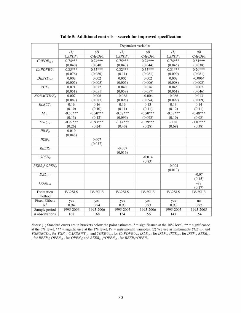
30

Table 5: Additional controls – search for improved specification Dependent variable:

(1) (2) (3) (4) (5) (6)

CAPDFit CAPDFit CAPDFit CAPDFit CAPDFit CAPDFit CAPDEi,t-1 0.74***

(0.040) 0.74*** (0.040)

0.75*** (0.043)

0.74*** (0.044)

0.74*** (0.045)

0.81*** (0.038)

CAPDFWYit 0.35*** (0.076)

0.35*** (0.080)

0.32*** (0.11)

0.35*** (0.081)

0.31*** (0.099)

0.20*** (0.081)

DEBTEi,t-1 0.002 (0.005)

0.002 (0.005)

0.005 (0.005)

0.002 (0.006)

0.003 (0.008)

-0.006* (0.003)

YGFit 0.071 (0.051)

0.072 (0.051)

0.040 (0.059)

0.076 (0.057)

0.045 (0.061)

0.007 (0.046)

NONACTIVEit 0.007 (0.087)

0.006 (0.087)

-0.068 (0.098)

-0.004 (0.094)

-0.066 (0.099)

0.013 (0.009)

ELECTit 0.16 (0.10)

0.16 (0.10)

0.16 (0.11)

0.13 (0.11)

0.13 (0.12)

0.14 (0.11)

Mi,t-1 -0.50*** (0.13)

-0.50*** (0.12)

-0.52*** (0.096)

-0.50*** (0.093)

-0.53*** (0.10)

-0.48*** (0.08)

SGPi,t-1 -0.92*** (0.26)

-0.93*** (0.24)

-1.14*** (0.40)

-0.79*** (0.28)

-0.88 (0.69)

-1.07*** (0.38)

IRLFit 0.010 (0.048)

IRSFit 0.007 (0.037)

REERit -0.007 (0.016)

OPENit -0.014 (0.83)

REERit*OPENit -0.004 (0.013)

DELi,t-1 -0.07 (0.15)

COMi,t-1 -28 (0.17)

Estimation method

IV-2SLS IV-2SLS IV-2SLS IV-2SLS IV-2SLS IV-2SLS

Fixed Effects yes yes yes yes yes no R2 0.94 0.94 0.93 0.93 0.93 0.92

Sample period 1995-2006 1995-2006 1995-2005 1995-2006 1995-2005 1995-2005 # observations 168 168 154 156 143 154

Notes: (1) Standard errors are in brackets below the point estimates, * = significance at the 10% level, ** = significance at the 5% level, *** = significance at the 1% level, IV = instrumental variables. (2) We use as instruments YGEi,t-1, and YGEOECDt-1 for YGFi,t; CAPDEWYi,t-1 and YGEWYi,t-1 for CAPDFWYi,t; IRLEi,t-1 for IRLFit; IRSEi,t-1 for IRSFit; REERi,t-

1 for REERit; OPENi,t-1 for OPENit; and REERi,t-1*OPENi,t-1 for REERit*OPENit.

31

Table 6: Alternative common driving factors

Dependent variable: (1) (2) (3) (4)

CAPDFit CAPDFit CAPDFit CAPDFit CAPDEi,t-1 0.74***

(0.041) 0.74*** (0.040)

0.74*** (0.040)

0.74*** (0.039)

CAPDFWYit 0.36*** (0.086)

0.33*** (0.10)

0.35*** (0.075)

0.36** (0.076)

DEBTEi,t-1 0.003 (0.005)

0.003 (0.005)

0.003 (0.005)

0.002 (0.005)

YGFit 0.057 (0.053)

0.068 (0.055)

0.071 (0.050)

0.073 (0.050)

YGFWYit 0.066 (0.11)

OILFt 0.048 (0.21)

IRLFWYAit 0.004 (0.058)

IRSFWYAit 0.015 (0.048)

NONACTIVEit 0.001 (0.087)

0.004 (0.087)

0.006 (0.087)

0.008 (0.087)

ELECTit 0.16 (0.10)

0.16 (0.10)

0.16 (0.10)

0.16 (0.10)

Mi,t-1 -0.48*** (0.090)

-0.48*** (0.092)

-0.49*** (0.10)

-0.49*** (0.096)

SGPi,t-1 -0.99*** (0.26)

-0.97*** (0.27)

-0.94*** (0.25)

-0.94*** (0.23)

Estimation method IV-2SLS IV-2SLS IV-2SLS IV-2SLS Fixed Effects yes yes yes yes

R2 0.94 0.94 0.94 0.94 Sample period 1995-2006 1995-2006 1995-2006 1995-2006

No. of observations 168 168 168 168

Notes: (1) Standard errors are in brackets below the point estimates, * = significance at the 10% level, ** = significance at the 5% level, *** = significance at the 1% level, IV = instrumental variables. (2) We use as instruments YGEi,t-1 and YGEOECDt-1 for YGFit; CAPDEWYi,t-1 and YGEWYi,t-1 for CAPDFWYit; OILEt-1 for OILFt; IRLEWYAi,t-1 for IRLFWYAit; and IRSEWYAi,t-1 for IRSFWYAit.

32

Table 7: Controls to capture indirect fiscal spill-overs

Dependent variable: (1) (2) (3)

CAPDFit CAPDFit CAPDFit CAPDEi,t-1 0.74***

(0.040) 0.74*** (0.040)

0.75*** (0.045)

CAPDFWYit 0.35*** (0.076)

0.35*** (0.080)

0.34*** (0.12)

DEBTEi,t-1 0.004 (0.005)

0.004 (0.005)

0.005 (0.005)

YGFit 0.072 (0.051)

0.076 (0.050)

0.025 (0.068)

NONACTIVEit 0.005 (0.087)

0.005 (0.087)

-0.065 (0.097)

ELECTit 0.16 (0.10)

0.16 (0.10)

0.16 (0.11)

Mi,t-1 -0.46*** (0.10)

-0.47*** (0.096)

-0.53*** (0.099)

SGPi,t-1 -1.00*** (0.25)

-0.97*** (0.24)

-1.11*** (0.41)

IRLFWYit -0.022 (0.050)

IRSFWYit -0.015 (0.052)

REERWYit -0.027 (0.051)

Estimation method IV-2SLS IV-2SLS IV-2SLS Fixed Effects yes yes yes

R2 0.94 0.94 0.93 Sample period 1995-2006 1995-2006 1995-2005

No. of observations 168 168 154

Notes: (1) Standard errors are in brackets below the point estimates, * = significance at the 10% level, ** = significance at the 5% level, *** = significance at the 1% level, IV = instrumental variables. (2) We use as instruments YGEi,t-1 and YGEOECDt-1 for YGFi,t; CAPDEWYi,t-1 and YGEWYi,t-1 for CAPDFWYi,t; IRLEWYi,t-1 for IRLFWYit; IRSEWYi,t-1 for IRSFWYit; and REERWYi,t-1 for REERWYit.

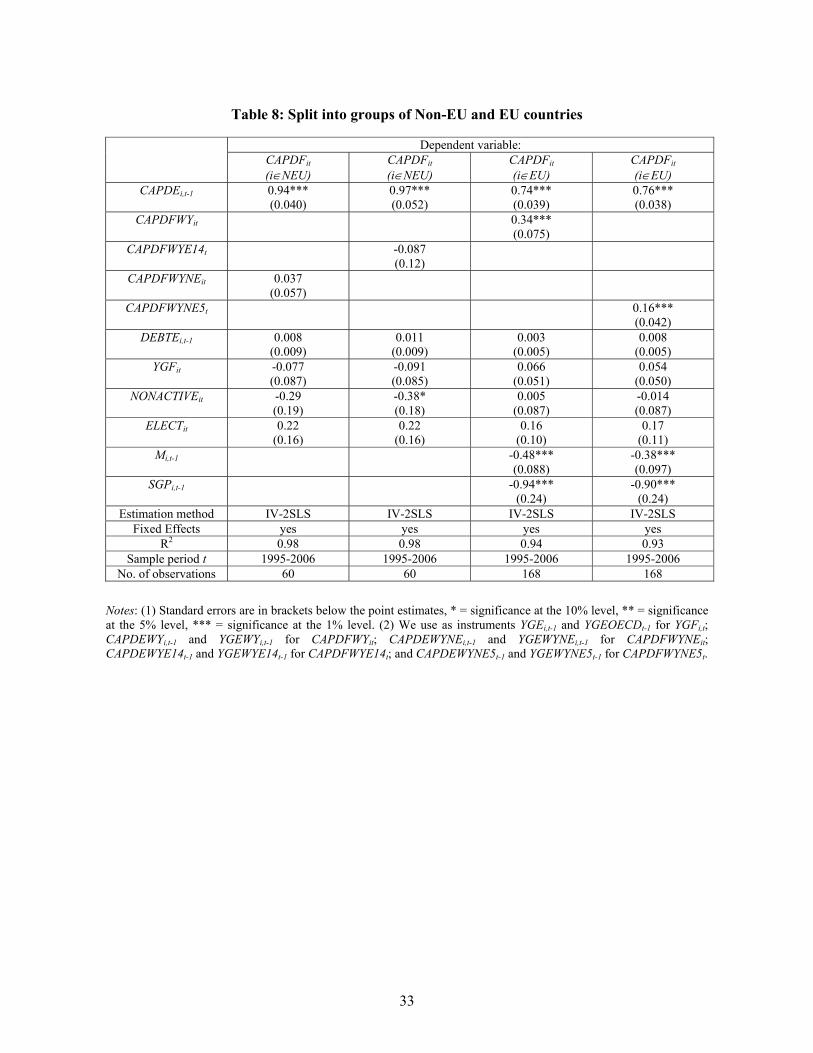
33

Table 8: Split into groups of Non-EU and EU countries

Dependent variable:

CAPDFit

(i∈NEU) CAPDFit

(i∈NEU) CAPDFit

(i∈EU) CAPDFit

(i∈EU) CAPDEi,t-1 0.94***

(0.040) 0.97*** (0.052)

0.74*** (0.039)

0.76*** (0.038)

CAPDFWYit 0.34*** (0.075)

CAPDFWYE14t -0.087 (0.12)

CAPDFWYNEit 0.037 (0.057)

CAPDFWYNE5t 0.16*** (0.042)

DEBTEi,t-1 0.008 (0.009)

0.011 (0.009)

0.003 (0.005)

0.008 (0.005)

YGFit -0.077 (0.087)

-0.091 (0.085)

0.066 (0.051)

0.054 (0.050)

NONACTIVEit -0.29 (0.19)

-0.38* (0.18)

0.005 (0.087)

-0.014 (0.087)

ELECTit 0.22 (0.16)

0.22 (0.16)

0.16 (0.10)

0.17 (0.11)

Mi,t-1 -0.48*** (0.088)

-0.38*** (0.097)

SGPi,t-1 -0.94*** (0.24)

-0.90*** (0.24)

Estimation method IV-2SLS IV-2SLS IV-2SLS IV-2SLS Fixed Effects yes yes yes yes

R2 0.98 0.98 0.94 0.93 Sample period t 1995-2006 1995-2006 1995-2006 1995-2006

No. of observations 60 60 168 168

Notes: (1) Standard errors are in brackets below the point estimates, * = significance at the 10% level, ** = significance at the 5% level, *** = significance at the 1% level. (2) We use as instruments YGEi,t-1 and YGEOECDt-1 for YGFi,t; CAPDEWYi,t-1 and YGEWYi,t-1 for CAPDFWYit; CAPDEWYNEi,t-1 and YGEWYNEi,t-1 for CAPDFWYNEit; CAPDEWYE14t-1 and YGEWYE14t-1 for CAPDFWYE14t; and CAPDEWYNE5t-1 and YGEWYNE5t-1 for CAPDFWYNE5t.

34

Table 9: Fiscal behaviour before and after the SGP came into force

Dependent variable: CAPDFit Pre-SGP Post-SGP

CAPDEi,t-1 0.68*** (0.049)

0.86*** (0.062)

CAPDFWYit 0.48*** (0.13)

0.23*** (0.089)

DEBTEi,t-1 -0.004 (0.005)

0.011 (0.008)

YGFit 0.077 (0.087)

0.038 (0.054)

NONACTIVEit 0.022 (0.085)

-0.011 (0.091)

ELECTit 0.29* (0.16)

-0.006 (0.14)

Mi,t-1 -0.40*** (0.15)

SGPi,t-1 -1.31*** (0.30)

Estimation method IV-2SLS Fixed Effects yes

R2 0.94 Sample period 1995-2006

No. of observations 168

Notes: (1) Standard errors are in brackets below the point estimates, * = significance at 10% level, ** = significance at 5% level, *** = significance at 1% level. (2) The instrumental variables regressions use as instruments YGEi,t-1 and YGEOECDt-1 for YGFi,t; and CAPDEWYi,t-1 and YGEWYi,t-1 for CAPDFWYit.

35

Table 10: Estimates of baseline fiscal rules with non-adjusted primary deficits Dependent variable:

(1) (2) (3)

PDFi,t

PDFi,t

PDFi,t

PDEi,t-1 0.74*** (0.040)

0.71*** (0.036)

0.72*** (0.037)

PDFWYi,t 0.19*** (0.060)

0.21*** (0.056)

CAPDFWYi,t 0.27*** (0.079)

DEBTEi,t-1 -0.012*** (0.005)

-0.014*** (0.003)

-0.014*** (0.003)

YGFi,t -0.077 (0.054)

Country- specific

Country- specific

NONACTIVEi,t 0.024 (0.098)

0.018 (0.067)

0.019 (0.065)

ELECTi,t 0.17 (0.11)

0.13* (0.079)

0.14* (0.079)

Mi,t-1 -0.44*** (0.091)

-0.48*** (0.058)

-0.46*** (0.058)

SGPi,t-1 -0.25 (0.26)

-0.074 (0.15)

-0.11 (0.15)

Estimation method

IV-2SLS IV-2SLS IV-2SLS

Fixed Effects yes yes yes R2 0.94 0.95 0.95

Sample period 1995-2006 1995-2006 1995-2006 No. of

observations 168 168 168

Notes: (1) Robust standard errors are in brackets below the point estimates, * = significance at the 10% level, ** = significance at the 5% level, *** = significance at the 1% level. (2) “Country-specific” means that the regression allows for country-specific coefficients. (3) We use as instruments CAPDEWYi,t-1 and YGEWYi,t-1 for CAPDFWYi,t; YGEi,t-1 and YGEOECDt-1 for YGFi,t; and PDEWYi,t-1 and YGEWYi,t-1 for PDFWYit.

36

Table 11: Split into groups of large and small countries

Dependent variable (1) (2) (3) (4) CAPDFit

(i∈L) CAPDFit

(i∈S) CAPDFit

(i∈L) CAPDFit

(i∈S) CAPDEi,t-1 0.83***

(0.067) 0.72*** (0.046)

0.83*** (0.062)

0.73*** (0.043)

CAPDFWYit 0.057 (0.10)

0.49*** (0.098)

CAPDFWYLit 0.076 (0.094)

CAPDFWYSit 0.49*** (0.081)

DEBTEi,t-1 0.002 (0.011)

0.001 (0.005)

0.003 (0.011)

-0.012** (0.006)

YGFit 0.12* (0.066)

0.12* (0.067)

0.12* (0.065)

0.074 (0.061)

NONACTIVEit -0.079 (0.16)

0.013 (0.11)

-0.073 (0.15)

0.057 (0.11)

ELECTit -0.007 (0.14)

0.18 (0.14)

-0.007 (0.14)

0.16 (0.14)

Mi,t-1 -0.45*** (0.10)

-0.44*** (0.17)

-0.45*** (0.10)

-0.67*** (0.17)

SGPi,t-1 0.29 (0.57)

-1.16*** (0.27)

0.19 (0.58)

-1.06** (0.25)

Estimation method IV-2SLS IV-2SLS IV-2SLS IV-2SLS Fixed Effects yes yes yes yes

R2 0.95 0.93 0.95 0.94 Sample period t 1995-2006 1995-2006 1995-2006 1995-2006

No. of observations 60 108 60 108 Notes: (1) Standard errors are in brackets underneath the point estimates, * = significance at the 10% level, ** = significance at the 5% level, *** = significance at the 1% level. (3) We use as instruments CAPDEWYi,t-1 and YGEWYit for CAPDFWYit; CAPDEWYLi,t-1 and YGEWYLi,t-1 for CAPDFWYLit; CAPDEWYSi,t-1 and YGEWYSi,t-1 for CAPDFWYSit; YGEi,t-1, YGEWYi,t-1 and YGEOECDt-1 for YGFi,t.

37

Table 12: Do groups of countries affect each other? Dependent variable

(1) (2) (3) (4) (5) (6) (7) (8)

CAPDFit

(i∈S) CAPDFit

(i∈L) CAPDFit

(i∈S) CAPDFit

(i∈L) CAPDFit

(i∈S) CAPDFit

(i∈S) CAPDFit

(i∈S) CAPDFit

(i∈S) CAPDEi,t-1 0.73***

(0.047) 0.86*** (0.077)

0.76*** (0.046)

0.82*** (0.059)

0.74*** (0.046)

0.74*** (0.044)

0.72*** (0.047)

0.74*** (0.046)

CAPDFWYL5t 0.46*** (0.10)

-0.095 (0.20)

0.54*** (0.17)

0.042 (0.24)

CAPDFWYSit 0.57*** (0.17)

0.55*** (0.10)

0.53*** (0.16)

CAPDFWYS9t -0.016 (0.10)

CAPDFWYNE5t 0.19*** (0.060)

0.061 (0.053)

-0.054 (0.070)

-0.059 (0.096)

-0.066 (0.089)

DEBTEi,t-1 0.004 (0.005)

-0.000 (0.011)

0.008 (0.006)

0.003 (0.011)

-0.015 (0.008)

-0.016** (0.008)

0.002 (0.006)

-0.016** (0.008)

YGFit 0.11 (0.070)

0.12* (0.070)

0.059 (0.073)

0.13** (0.063)

0.063 (0.073)

0.055 (0.069)

0.10 (0.071)

0.061 (0.072)

NONACTIVEit 0.001 (0.11)

-0.094 (0.16)

-0.028 (0.11)

-0.057 (0.15)

0.065 (0.11)

0.067 (0.11)

0.007 (0.11)

0.067 (0.12)

ELECTit 0.19 (0.14)

-0.027 (0.14)

0.21 (0.15)

0.003 (0.14)

0.16 (0.14)

0.15 (0.14)

0.19 (0.14)

0.15 (0.14)

Mi,t-1 -0.40** (0.18)

-0.44*** (0.11)

-0.34* (0.19)

-0.41*** (0.11)

-0.72*** (0.19)

-0.75*** (0.20)

-0.44*** (0.19)

-0.74*** (0.20)

SGPi,t-1 -1.17*** (0.28)

0.47 (0.54)

-1.02*** (0.28)

0.12 (0.57)

-1.02*** (0.26)

-1.04*** (0.25)

-1.19*** (0.28)

-1.05*** (0.26)

Estimation method

IV-2SLS IV-2SLS IV-2SLS IV-2SLS IV-2SLS IV-2SLS IV-2SLS IV-2SLS

Fixed Effects yes yes yes yes yes yes yes yes R2 0.93 0.95 0.92 0.95 0.94 0.94 0.93 0.94

Sample period t 1995-2006 1995-2006 1995-2006 1995-2006 1995-2006 1995-2006 1995-2006 1995-2006 No. of

observations 108 60 108 60 108 108 108 108

Notes: (1) Standard errors are in brackets below the point estimates, * = significance at the 10% level, ** = significance at the 5% level, *** = significance at the 1% level. (2) We use as instruments CAPDEWYSi,t-1 and YGEWYSi,t-1 for CAPDFWYSit; CAPDEWYLi,t-1 and YGEWYLi,t-1 for CAPDFWYLit; CAPDEWYS9t-1 and YGEWYS9t-1 for CAPDFWYS9t; CAPDEWYL5t-1 and YGEWYL5t-1 for CAPDFWYL5t; CAPDEWYNE5t-1 and YGEWYNE5t-1 for CAPDFWYNE5t; and YGEi,t-1 and YGEOECDt-1 for YGFit.

38

Figures

Figure 1: Regression fit versus actual values of the deficit forecast

-4

-3

-2

-1

0

1

2

95 96 97 98 99 00 01 02 03 04 05 06

CA PDF CAPDF F

_AUT

-7.0

-6.5

-6.0

-5.5

-5.0

-4.5

-4.0

95 96 97 98 99 00 01 02 03 04 05 06

CAPDF CA PDFF

_BEL

-3.0

-2.5

-2.0

-1.5

-1.0

-0.5

0.0

0.5

95 96 97 98 99 00 01 02 03 04 05 06

CAPDF CAPDFF

_DEU

-5

-4

-3

-2

-1

95 96 97 98 99 00 01 02 03 04 05 06

CAP DF CAPDFF

_DNK

-3.6

-3.2

-2.8

-2.4

-2.0

-1.6

-1.2

95 96 97 98 99 00 01 02 03 04 05 06

CA PDF CAPDF F

_ESP

-6

-5

-4

-3

-2

-1

0

1

2

3

95 96 97 98 99 00 01 02 03 04 05 06

CAPDF CA PDFF

_FIN

-1.6

-1.2

-0.8

-0.4

0.0

0.4

0.8

95 96 97 98 99 00 01 02 03 04 05 06

CAPDF CAPDFF

_FRA

-4

-3

-2

-1

0

1

2

95 96 97 98 99 00 01 02 03 04 05 06

CAP DF CAPDFF

_GBR

-8

-7

-6

-5

-4

-3

-2

-1

0

95 96 97 98 99 00 01 02 03 04 05 06

CA PDF CAPDF F

_GRC

-6

-5

-4

-3

-2

-1

0

1

2

95 96 97 98 99 00 01 02 03 04 05 06

CAPDF CA PDFF

_IRE

-7

-6

-5

-4

-3

-2

-1

0

95 96 97 98 99 00 01 02 03 04 05 06

CAPDF CAPDFF

_ITA

-3.6

-3.2

-2.8

-2.4

-2.0

-1.6

-1.2

95 96 97 98 99 00 01 02 03 04 05 06

CAP DF CAPDFF

_NLD

-2.8

-2.4

-2.0

-1.6

-1.2

-0.8

-0.4

0.0

95 96 97 98 99 00 01 02 03 04 05 06

CA PDF CAPDF F

_PR T

-6

-4

-2

0

2

4

6

95 96 97 98 99 00 01 02 03 04 05 06

CAPDF CA PDFF

_SWE

Note: this figure is based on the specification in Column 5 of Table 2 and depicts the actual forecast, CAPDF, in black and its regression fit, CAPDFF, in grey.

39

Figure 2 Time Effects versus ‘external’ fiscal factors

-4.00

-3.50

-3.00

-2.50

-2.00

-1.50

-1.00

-0.50

0.00

0.50

1.00

1995 1996 1997 1998 1999 2000 2001 2002 2003 2004 2005 2006

-0.60

-0.40

-0.20

0.00

0.20

0.40

0.60

0.80

CAPDFWY CAPDFWD YGFOECD time effect 1995-2006