Submitted to The Astronomical Journal, 5 December 2002

On the Redshift Distribution of Long-Duration Gamma-Ray Bursts

J. S. Bloom1,2

1 Harvard Society of Fellows, 78 Mount Auburn Street, Cambridge, MA 02138 USA

2 Harvard-Smithsonian Center for Astrophysics, MC 20, 60 Garden Street, Cambridge, MA02138, USA

ABSTRACT

The 26 long-duration gamma-ray bursts (GRBs) with known redshifts form a distinctcosmological set, selected differently than other cosmological probes such as quasarsand galaxies. Since the progenitors are now believed to be connected with active star-formation and since burst emission penetrates dust, one hope is that with a uniformly-selected sample, the large-scale redshift distribution of GRBs can help constrain the star-formation history of the Universe. However, we show that strong observational biases inground-based redshift discovery hamper a clean determination of the large-scale GRBrate and hence the connection of GRBs to the star formation history. We then focuson the properties of the small-scale (clustering) distribution of GRB redshifts. Whencorrected for heliocentric motion relative to the local Hubble flow, the observed redshiftsappear to show a propensity for clustering: eight of 26 GRBs occurred within a recessionvelocity difference of 1000 km s−1 of another GRB. That is, four pairs of GRBs occurredwithin 30 h−1

65 Myr in cosmic time, despite being causally separated on the sky. Weinvestigate the significance of this clustering using a simulation that accounts for at leastsome of the strong observational and intrinsic biases in redshift discovery. Comparisonof the numbers of close redshift pairs expected from the simulation with that observedshows no significant small-scale clustering excess in the present sample; however, thefour close pairs occur only in about twenty percent of the simulated datasets (the precisesignificance of the clustering is dependent upon the modeled biases). We conclude withsome impetuses and suggestions for future precise GRB redshift measurements.

Subject headings: cosmology: miscellaneous — cosmology: observations — gamma rays:bursts

1. Introduction

A growing body of evidence suggests that long-duration GRBs arise from the death of massivestars. If true, the large-scale redshift distribution of GRBs should trace the star-formation history

brought to you by COREView metadata, citation and similar papers at core.ac.uk

provided by CERN Document Server

– 2 –

of the Universe (Totani 1997; Wijers et al. 1998; Lamb & Reichart 2000; Porciani & Madau 2001;Bromm & Loeb 2002). And, as explosive and transient events detectable to high redshift, GRBsclearly offer a probe of the Universe that is distinct from other lighthouses (Loeb 2002). Already,GRBs have helped shed light on the nature of damped Lyman α absorbers (?, e.g.,)]fmt+02 and thenature of the faint end of the luminosity function of galaxies at moderate redshifts (?, e.g.,)]dkb+01.

As a redshift sample selected from an apparent isotropic population and from hosts spanningthe breadth of the galaxy luminosity function, GRBs have the potential to provide a unique censusof the redshift distribution of matter in the Universe. Not only can the large-scale distribution ofGRBs help constrain the star-formation rate (SFR), but, in a manner complementary to pencil-beam surveys and magnitude-limited galaxy and quasar surveys, the small-scale distribution canhelp test hypotheses and observational suggestions about clustering and periodicity of sources inredshift space.

Given the penetrative powers of GRBs through dust, several studies have attempted to comparethe large-scale redshift distribution of GRBs with the SFR obtained by other means (Schaefer et al.2001; Lloyd-Ronning et al. 2002a; Stern et al. 2002; Norris 2002). Such studies focused on usingthe prompt γ-ray properties of BATSE bursts, calibrated with some measured GRB redshifts, todetermine the bursting rate. With so few actual redshifts measured, each of which were measuredunder different observational constraints, the task of distinguishing different SFR scenarios fromthe sparsely sampled GRB rate is considerably challenging. Indeed we show herein, that when theobservational biases in redshift determination are taken into account, several proposed forms forthe universal SFR cannot be distinguished.

Investigation of the small-scale distribution of GRBs has not been presented thus far. Ofparticular interest is whether the clustering properties in redshift space are significant in lightof the observational biases and the intrinsic redshift distribution. Do GRBs occur at preferredredshifts? There is enough historical, albeit controversial, evidence to warrant an investigationof the significance of special redshifts in the Universe using GRBs. Broadhurst et al. (1990), forinstance, found evidence for periodicity of clustering of redshifts on 128 h−1 Mpc scales in twopencil-beam surveys. While excess power on these scales has not been definitively confirmed inhigher-redshift studies (e.g., with the 2dF redshift survey: Hawkins et al. 2002; although see Gal &Djorgovski 1997 and Duari et al. 1992) the Broadhurst et al. result may be statistically significantin comparison with N -body simulations (Yoshida et al. 2001). But, as Yoshida et al. emphasize,large clusters in a galaxy sample tend to accentuate the appearance of excess power at certainscales1. A GRB sample does not suffer such a bias since bursts occur in regions of space that are

1Excess power on such 128 h−1 Mpc scales could be an imprint of a primordial density fluctuation (Dekel et al.

1992). As a statistical measure, if this interpretation is true, then the same redshifts with over-densities would not

reoccur in surveys that sample different directions on the sky. However, specific special redshifts would be preferred

if the observed power arises by more exotic means. For example, oscillations of the scalar potential (Morikawa 1991)

or the gravitational constant (Salgado et al. 1996) induce an oscillation in the Hubble constant versus cosmic time.

The result is an apparent clustering of sources in redshift space at epochs where the expansion temporarily slows.

– 3 –

gravitationally (and causally) disconnected.

The focus of this paper is on the small-scale (clustering) distribution of GRB redshifts. Inaddition we examine the large-scale distribution of GRB redshifts, and note the difficulty in de-termining the global GRB rate due to the small sample and strong observational biases. In §2 wepresent the GRB redshift sample for 26 bursts, corrected for the heliocentric motion through thelocal Hubble flow and construct an observationally-motivated probability distribution for redshiftdiscovery. In §3, we compare the large-scale distribution of GRB redshifts with that expected fromthe observing biases and an intrinsic rate distribution. After showing the insensitivity of the presentsample to distinguishing various SFRs, and under the anzatz that GRBs should trace the SFR, wefix a model for redshift discovery probability that adequately reproduces the universal SFRs. Usingthis distribution, we then test the significance of the number of observed pairs of GRBs with smallrecession velocity differences. We conclude with a discussion about the importance and usefulnessof conducting precise redshift measurements for future GRBs.

2. The Redshift Sample

Table 1 presents a summary of the sky location and observed redshifts associated with 26cosmological GRBs, in order of increasing redshift. The highest observed redshift system derivedusing absorption or emission features with the highest reported accuracy is given in column seven.The line features used to measure the reported redshift are given in column six. Absorption-lineredshifts, which place a strict lower limit to the actual GRB redshift, are found when a spectrum ofthe afterglow is absorbed by metal-line systems along the line of sight. Emission-line redshifts arederived from spectroscopy of the galaxy associated with the GRB position, either found promptly,superimposed with the spectrum of the transient afterglow (e.g., 980703; Djorgovski et al. 1998),or at later times, when the afterglow light has faded. Nineteen sources in the sample have mea-sured emission-line redshifts, and 12 have absorption-line redshifts. The uncertainty in the redshiftmeasurements are usually provided in the literature, but where none were provided we assumed anerror of 10 percent in the least significant digit reported.

Since we are interested in testing the observed rate and redshift distribution of GRBs againstdifferent models for star-formation and small-scale clustering, we now discuss the observationalbiases in GRB detection, localization, and finally, redshift determination.

2.1. Biases in GRB Detection

If GRBs arise in collimated emission, then the relativistic Doppler beaming allows for detectionof a GRB only if the detector lies in the direction of the cone of emission. By studying the openingangles of those GRBs which have been detected, it is reckoned that only about one in every fivehundred GRBs are detectable at (i.e., pointed toward) Earth due to beaming (Frail et al. 2001).

– 4 –

Of those bursts that are beamed toward Earth, only those that reach a certain critical fluxlevel will be detected by the triggering algorithms of a given satellite. The typical threshold foron-board detection in the BATSE catalog is a peak flux of a 0.3 photon cm−2 s−1 (in ’t Zand& Fenimore 1994; Pendleton et al. 1998). In finding that the total energy release in GRBs isapproximately constant, Frail et al. (2001) showed that bursts that are more highly collimatedappear to be intrinsically brighter (in flux/fluence per unit solid angle). Thus, for a scenario whereGRBs are jetted and release about the same amount of electromagnetic energy, brighter burststend to be more distant. As clear illustration of this, note that the peak flux of the highest redshiftburst, GRB 000131 (z = 4.5), was at the top 5% of the entire BATSE catalogue (Andersen et al.2000).

This somewhat counterintuitive trend implies that the brightest GRBs can be detected toextremely high redshifts, certainly beyond the age of reionization (z ∼ 7). More important for thepresent study is that Malmquist bias should play little role in diminishing the observed burst rateat high-redshift: bursts significantly fainter (by up to ∼ 10−3) than GRB000131 could have beendetected at similar redshifts.

Using the prompt high-energy properties, irrespective of individual burst redshifts, it has beenshown that the brightness distribution of GRBs is consistent with a broad range of star-formationrates and luminosity functions (?, e.g.,)]lw98,klk+00,sch01,sts02. Using distance indicators cali-brated from a sub-set of the bursts with known redshift, Lloyd-Ronning et al. (2002b) claimed thatthe GRB rate increases monotonically at least out to z ≈ 10. In our opinion, this suggestion pointsmore to the pitfalls of extrapolating GRB distance indicators beyond the redshift range in whichthey were calibrated, than revealing concrete properties of the high-redshift bursting rate density.Another approach to constrain the burst rate, which we attempt herein, is to use only those burstswith actual measured redshifts.

2.2. Biases in Afterglow Localization

For those GRBs that are triggered and rapidly localized using the prompt X-rays or γ-rays, theobserving community tries to determine a sub-arcsec position and ultimately associate a redshift viahost or absorption-line spectroscopy. This is accomplished by first identifying a transient afterglow.

Three major biases are important for afterglow discovery. First, GRBs will be preferentiallylocalized if they occur at a time and place in the sky where ground- or space-based telescopes canrapidly observe the prompt burst position with large enough fields–of–view. Second, only GRBafterglows with brightnesses above a given threshold for the particular afterglow-discovery observa-tions will be localized. Last, only GRB afterglows that are not heavily extincted by dust obscurationwill be first localized at optical wavelengths. Clearly, radio and X-ray afterglow discoveries do notsuffer this third bias. The existence of a population of dark bursts (Djorgovski et al. 2001a; Piroet al. 2002), those bursts without detectable optical afterglow emission, is clearly a result of all

– 5 –

three biases. (The current dark burst debate resolves around the relative importance of dust versusobservational biases in the manifestation of dark bursts (Berger et al. 2002; Fynbo et al. 2001).)

Since, for now, GRBs with redshifts are preferentially those that were first localized at opticalwavelengths (all but 970828, 980329, and 000210 were first localized at optical wavelengths), it seemsappropriate to suppose that a population of optically-localized GRBs should trace a star-formationrate derived from other optically-selected samples; Porciani & Madau (2001) have provided a pa-rameterized version of a SFR based upon the un-dust corrected Hubble Deep Field measurements(model SF1); in this model the SFR drops beyond z ∼ 2. In future GRB redshift samples of burststhat are first localized at radio, X-ray or even infrared wavelengths, the expectation is that theobserved rate will more closely trace the true (high mass) SFR in the universe.

2.3. Biases in Redshifts Determination

For those GRBs that are triggered and localized, most are followed up spectroscopically. Ifan absorption or emission-line redshift is found, it is of interest to know the relationship betweenthis and the true GRB redshift. A definitive measure of burst redshifts would need to connect thebursting location with some stationary gas local to the GRB, resulting in a detection of transientfeatures. To date, no transient absorption or emission features at optical wavelengths features havebeen associated with a GRB afterglow. Transient features, consistent with (later-time) opticalspectroscopic redshift measurements, have been seen in a prompt burst spectrum (Amati et al.2000; Le Floc’h et al. 2002) and a handful of X-ray afterglow spectra (?, e.g.,)]pcf+99,pggs+00.At present, the uncertainties in these X-ray-derived redshifts are orders of magnitude larger thanthose found typically at optical wavelengths. Perhaps more important, redshifts derived purely fromX-ray spectroscopy are contaminated from an unknown (potentially relativistic) outflow speed ofthe emitting or absorbing material; thus, precise measurements of the systematic redshift of GRBprogenitors are best determined using the UV and optical features of host HII regions and/orintervening host clouds.

The equivalent widths of the highest redshift absorption systems in GRB afterglows are signif-icantly larger than systems seen though quasar lines–of–sight (?, e.g.,)]svk+02. This is naturallyunderstood in the context of the prevailing progenitor model, namely that long-duration burstsarise from the death of massive stars and, owing to the rapid evolution of massive stars, GRBexplosion locations should be in or near relatively dense regions of active star-formation. Thus,GRBs should reside in or near the region that gives rise to the gas absorption. Consistent with thispicture is the observation that well-localized GRBs, a subset of which comprises the present sam-ple, have been observationally connected to the location of the light of the putative host galaxies(Bloom et al. 2002).

The probability of a spurious (spatial) association of an afterglow with its putative host hasbeen shown to be small (∼< 10−2) for most bursts. In fact in a sample of 20 GRBs with arcsecond

– 6 –

localizations, statistically, at most a few spatial associations could have been spurious (Bloomet al. 2002). Therefore, from the location argument, GRB redshifts determined from emission linespectroscopy of the hosts are likely to be close to the true systematic velocities of the progenitor;at most, we would expect a velocity offset on the order of a few hundred km s−1 from the motion ofthe progenitor system about its host. Likewise, unless the afterglow light pierces some high-velocityoutflowing material, absorption-line redshifts should also provide a accurate measure of the trueGRB redshift. Perhaps most convincing that measured redshifts are closely related to the realsystemic redshifts, is that of the five GRBs with both emission and absorption line spectroscopy,the highest redshift absorption system is always found to be consistent with the emission-lineredshift of the host.

2.4. Correcting the measured redshifts for heliocentric motion relative to the localHubble frame

One striking feature of the current redshift sample is the small apparent redshift differences, onthe order of a thousand km s−1, between some bursts from different sky locations and a apparentlyrandom trigger dates (differences of 6 months to 5 years). (Unlike in pencil-beam surveys theproximity in redshift can have nothing to do with systems, such as galaxies in clusters, that are incausal contact.) These small velocity differences are comparable to the velocity of the Solar Systemthrough the local Hubble frame, and so a correction for this systematic motion is warranted. Suchmotion was measured by the angular dependence of temperature variations in the Cosmic MicrowaveBackground (CMB) with the COBE satellite (Smoot et al. 1991; Fixsen et al. 1994). This measuredvelocity (V = 365 ± 18 km s−1) and direction (toward Galactic coordinates l = 264.4 ± 0.3 deg,b = 48.4 ± 0.5 deg; Fixsen et al. 1994) are due to vector sum of the heliocentric motion about theGalactic center, the peculiar motion of the Milky Way in the Local Group and the Local Groupin-fall. We assume that all reported redshifts have been corrected to the heliocentric redshifts; thiscorrection is at most of order tens of km s−1 and so this assumption is relatively unimportant.

In order to remove this systematic bias from a measured redshift z, we find the angle (θCMB)between the GRB position and the heliocentric motion through the CMB; we then find the projectedheliocentric velocity toward the GRB as v,proj = V cos θCMB. If uc is the uncorrected apparentrecession velocity of a distant source, then, from the definition of redshift and the formula forrelativistic velocity addition, the corrected redshift in the local Hubble frame (lhf) is found from:

(1 + zlhf)2 =1 + uv,proj/c + u + v,proj/c

1 + uv,proj/c− u− v,proj/c, (1)

with the uncorrected apparent recession velocity as,

u =(1 + z)2 − 1(1 + z)2 + 1

. (2)

The calculated values of zlhf are given in column eight of Table 1. The associated uncertainties arederived by error analysis of equation 1, assuming that the errors on V and θCMB are uncorrelated

– 7 –

and noting that the fractional error on θCMB is significantly smaller than the fractional error onV. As seen in Table 1, for all but the most accurately measured redshifts, this correction addsnegligibly to the fractional error of the redshift.

3. Results

Table 2 shows the absolute difference in redshift and recession velocity of each burst matchedwith the burst that is closest in apparent recession velocity. Figure 1 shows this distribution of“nearest neighbor” apparent recession velocity differences versus redshift. The smallest groupingsoccur around redshift of unity, where the density of known GRB redshifts is highest. Four pairsare closer than ∼1000 km s−1 (0.0034 c) in redshift space2, and the largest velocity difference isbetween the two highest redshift bursts (|∆v| = 0.22 c).

Interestingly, the velocity differences of the four closest burst pairs (at redshifts z =0.692, 0.844,0.961, and 2.035) fall within the velocity dispersion of a large cluster of galaxies—and so, given theunknown peculiar velocity of the GRB hosts and the progenitor system within the hosts, these closeburst pairs are consistent with having occurred at the same cosmic time. Even assuming no peculiarvelocities of GRB progenitors relative to their local Hubble flow, eight of 26 GRBs occurred within30 h−1

65 Myr of another GRB. This was determined by computing the look-back times between thefour close pairs and assuming a cosmology with H0 = 65 km s−1 Mpc−1, ΩΛ = 0.7 and Ωm = 0.3.This cosmology is assumed throughout the paper where needed.

3.1. Simplistic probability calculation

How significant is this proximity in cosmic time? The bursts listed in Table 1 have been de-tected with recession velocities in the range vlow = 0.30 c (GRB 011121) to vhigh = 0.94 c (GRB 000131).In an ensemble of n bursts, assuming uniform probability of a GRB occurring and being detectedbetween vlow and vhigh, the probability that given pair of successive bursts are not as close as adistance ∆vc is P = exp (−n (vhigh − vlow)/∆vc). Therefore, the probability that at least one closepair exists in the ensemble, is,

P (1) = 1− Pn−1 (3)

For ∆vc = 1000 km s−1 and n = 26, the probability of at least one close pair with ∆v ≤ 1000 kms−1 is 0.967. The probability of at least one close pair with at most the smallest velocity differencein the observed GRB sample (∆vc = 259 km s−1) is 0.585. Both these probabilities thus indicate

2Of the eight bursts in the close four pairs, six redshifts were determined via emission lines from the putative host

galaxies. One redshift (GRB000926) was one with absorption spectroscopy only and another redshift (GRB000301C)

was found with both emission and absorption spectroscopy.

– 8 –

that there is nothing particularly unusual about the occurrence of at least one close pair in thecurrent sample.

In general, the probability that exactly k pairs are close can be approximated as,

P (k) ≈[n (vhigh − vlow)

∆vc

]k Pn−1 × n!(n− k)! k!

. (4)

For the present sample, there are k = 4 close pairs. Using this simplistic calculation we thereforeexpect four pairs to occur by random chance in 18.6% of samples. We have verified this approxima-tion by a Monte Carlo simulation, selecting n bursts uniformly over the range [vlow, vhigh]; however,this approximation breaks down for large velocity differences as it does not account for relativisticvelocity subtraction between successive bursts in velocity space.

3.2. Probability calculation with a model distribution

The above probability estimate does not take into account some important observational andendemic biases. First, the rate of GRBs is not uniform in redshift or recession velocity space.Instead, we expect GRBs to trace (or at least approximate) the star-formation rate (Totani 1997;Wijers et al. 1998), so that the peak of bursting activity should occur around z ∼ 1− 2. This willmake close velocity pairs more likely at redshifts near unity. Second, the chance that a burst willbe localized well enough to follow-up with spectrometers is not uniform in redshift. Instead, thischance depends, for optical localizations, sensitively on the native dust obscuration of the afterglow(see §2.2). Third, observing conditions and instrumentation play a strong role in determiningwhether the redshift of a GRB can be detected at that redshift. Most important, emission linesand absorption lines falling outside the broadband spectral coverage hamper the ability to detectredshifts (this may be an explanation for why no redshifts have been detected for 980519, 980326,and 980329). Even if a redshifted line falls within the spectral range, the presence of night sky linesmake detection of redshifts at certain wavelengths more unlikely. Fourth, instrumental sensitivityvaries across the spectral range and from instrument to instrument, night to night, and airmass toairmass.

Since we wish to know how the observed redshift sample compares with that expected giventhe above considerations we construct a toy probability model, P (z), giving the differential prob-ability that a burst at redshift z could ultimately yield a redshift measurement. We construct aglobal (rather than individual) distribution, neglecting the instrumental sensitivity differences fromburst to burst and the non-negligible chance that a redshift will be incorrectly assigned even afterthe detection of one or more spectral features. We use several parametrized versions of the starformation rate (SFR) from Porciani & Madau (2001). The overall shape of the distribution, PG(z),is then proportional to the number of bursts per unit redshift per unit observer time; that is, PG(z)

– 9 –

is proportional to the co-moving volume element and the co-moving SFR (ρSFR) versus redshift:

PG(z) ∝ dN

dt dz∝ ρSFR

1 + z

dV

dz

∝(

exp(3.4 z)exp(3.8 z) + 45

)× d2

L(z)(1 + z)3

√Ωm(1 + z)3 + Ωk(1 + z)2 + ΩΛ

, (5)

following eqs. [2]–[4] in Porciani & Madau (2001). Here dL(z) is the luminosity distance andΩm + Ωk + ΩΛ = 1. The factor of (1 + z) in the denominator accounts for the time dilation ofthe co-moving GRB rate. Following the discussion in §2.2, we have nominally chosen the un-dustcorrected SFR from Porciani & Madau (2001) (SF1). We also explore the two other models forPG(z) in Porciani & Madau (2001). In our model we do not take into account any biases relatedto the distance of the source in localization (in §2.2 we argued that there should be little biasin triggering based on distance). However, because of the observed anti-correlation between jetopening angles and prompt emission fluence (Frail et al. 2001), and the theoretical correlationbetween prompt burst emission and afterglow luminosity (Panaitescu et al. 2001), aside from dustobscuration, the afterglow from triggered GRBs that originate from higher redshift GRBs shouldnot be significantly dimmer at the same observer time (see also Ciardi & Loeb 2000; Lamb &Reichart 2000).

Nevertheless, if there is any dependence of triggering/localization on dL, we can try to accountfor such using a probability function related to luminosity distance, PL(z). There is also a cleareffect of distance upon redshift discovery: once a burst afterglow is localized and a spectrum isacquired, the detectability of emission features is diminished with increasing luminosity distance(nominally as d−2

L ). Systematically, only GRB hosts with higher rates of unobscured star formationwill be detectable at higher redshifts for a given integration time. For a given afterglow brightness,the distance bias does not exist for absorption-redshift GRBs as long as the particular redshiftedline is observable in the spectrum. To try to account for these elusive effects, we take the probabilityof redshift discovery due to distance [PL(z)] as unity from z = 0 to zl, decreasing with dL to somepower L. Nominally we take the values of zl = 1 and L = −2 but allow these quantity to vary inour modeling (see §3.3).

Using the observability of emission and absorption lines in the spectral range and in thepresence of night skylines, we construct a relative probability of redshift detection, PS(z). We takethe spectrum range as 3800–9800 A and assume a redshifted line is not observable if it falls withina wavelength that is half the instrumental resolution of a strong sky line listed in Osterbrock &Martel (1992). Here, we assume the instrumental resolution of 5 A (dispersion of ∼2.5 A/pixel).Based upon Table 1, we assume that a redshift can be obtained unambiguously with the detectionof at least one of four star-formation emission features: Ly α λ1216 A, [O II] λλ3727 A, Hα 6563A, and [O III] λλ 4959, 5008 A. Also based on Table 1, for redshifts based upon absorption featuresonly, we require that at least three of the following lines are detectable: Fe II λ2344.2 A, Fe II λ

2374.5 A, Fe II λ 2382.8 A, Fe II λ 2586.7 A, Fe II λ 2600 A, Mg II λλ 2796.4, 2803.5 A, Mg I λ

2853.0 A. If no redshifted star formation line nor prominent absorption line is observable at a given

– 10 –

redshift, z0, then we set PS(z0) = 0. Even if a line is observable, it may be too weak in emission ortoo low in equivalent width to be detected. Therefore with less and less lines observable at a givenz, the value of PS(z) should be diminished.

Figure 3 shows our toy model for PS(z), based upon the above considerations. We stress thatthis is a toy model for ground-based optical spectroscopy. Different instruments will provide free-spectral ranges that differ from our nominal range (3800–9800 A). The resolution of each instrumentalso will also particularly affect the observability of faint, narrow emission/absorption features inthe presence of sky lines. A moderate-resolution spectrograph (R ∼> 10000) should allow for featuredetection closer in wavelength to a sky line; even features which partially overlap a skyline couldbe detectable (?, e.g.,)]bbk+02.

The resultant relative probability distribution of detecting an optical redshift for a triggeredGRB is constructed as P (z) = PG(z) × PS(z) × PL(z) and is depicted in Figure 4. The relativeprobability distribution was calculated in bins of δz = 0.001. As can be seen in the normalizedcumulative distributions shown in Figure 2, the overall shape of the cumulative distributions arelargely unaffected by the sky lines. The most pronounced feature in P (z) is the drop in detectionprobability from z ≈ 1.5 − 2, due to the inaccessibility of strong emission lines in the opticalbandpass. The relative probability for detection of bursts at the redshift of GRB 980425 (z =0.0088) is exceedingly small and thus serves to emphasize the distinction between GRB 980425and the other long-duration GRBs with known redshift (?, e.g.,)]gvv+98,bkf+98,schm00,pm01. Assuch, we have not included GRB 980425 in our analysis.

3.3. Consistency of the Large-Scale GRB Distribution Differing SFR Models

As shown in Figure 2, the large-scale shape of the observed redshift distribution is adequatelydescribed by the model for L = −2, with the KS probability that the observed deviations areconsistent with a random selection from the model of PKS = 0.76 (SF1), 0.65 (SF2), and 0.54(SF3). Models where no account for the observational bias of detecting emission lines from high-redshift GRB hosts (L = 0) are clearly ruled out. While there are small differences in the KSprobability between various models for the star-formation rate, such models cannot be statisticallydistinguished by the current sample of GRBs with known redshifts. However, given the low KSprobabilities for L = 0, the data do support the notion that the observational biases of detectingemission lines from high-redshift GRB hosts must be taken in account. Note that a fairly largerange of L values (≈ −1 to −3 for SF1) yields a KS consistency with the data.

How sensitive are these results to our toy model for PS(z) and PL(z)? Changing the value ofzl we still get acceptable (but lower) KS statistics for L = −2: PKS = 0.20 (zl = 0.5; SF1), 0.22(zl = 1.25; SF1), 0.04 (zl = 1.5; SF1). With zl > 4.5, the L = −2 case is effectively equivalent tothe L = 0 case (PKS = 0.003 for zl = 5; SF1). By removing the effect of the sky lines and limitedfree-spectral range in redshift determination, the KS statistics are still acceptable, albeit with lower

– 11 –

values of the KS statistic: PKS = 0.37 (SF1), 0.19 (SF2), 0.10 (SF3).

3.4. Testing the Small-Scale GRB Redshift Distribution

Assuming that GRBs do trace the global star-formation rate we fix the form of PL(z) that givesa reasonable agreement with all three SF models. From here, we can test the significance of thesmall-scale clustering properties. To do so, we produce a Monte Carlo realization as sets of GRBredshifts drawn from the probability for redshift detection P (z) for each SFR model. We simulated5000 iterations of sets of GRB redshifts. For each iteration, 26 bursts were selected uniformly from[0,1] and then mapped to redshift using the cumulative distribution, interpolating between bins toincrease the resolution.

We thought of no obvious existing statistic to compare the small-scale redshift structure ofthe observed distribution with the Monte Carlo set. However, since one feature is the existence ofsuch close redshift pairs we can ask how often such numbers of pairs are found in the distribution.Table 3 summarizes the results of the comparison. Column two lists the number of observed GRBswithin an apparent recession velocity of |∆v| of another GRB. Columns three, four and five givethe probability of such occurrences in the simulated distributions for the three different GRB rates,PG(z). Following the table, the simulation predicts that at least two bursts (one pair) should occurby random chance in 53% of real world samples for the smallest observed velocity difference. Thisis close to the probability obtained in our simplistic calculation (59%) in §3.1. For ∆v values near1000 km s−1, the probability drops to ≈19% before rising again at large velocity offsets. Therefore,despite the apparent close pairings in redshift space, we find no significant small-scale redshiftclustering in the present sample.

Note, however, this comparison only references 2-point correlations. Following column eight ofTable 1 and column 6 of Table 2, there are two groupings of three bursts within 2500 km s−1 (atz = 0.69 and z = 0.84). Using the Monte Carlo set, the probability of getting 2 groupings of threebursts within 2500 km s−1 is 0.24 (SF1), 0.17 (SF2), and 0.13 (SF3). Again, the present sampleshows no evidence for significant multi-burst clustering.

With the advent of Swift3, it is not unreasonable to expect upwards of one hundred new GRBredshifts within the next several years. As the density of redshifts increases, the number of closeredshift pairs (and triples) will certainly increase. Commensurately, for an expanded sample to yieldsignificant clustering results, the number of close pairs must increase. Using the present models, asa function of bursts in a sample, we predict the required number of observed close pairs in orderto be considered a significant excess above a random sample. Figure 5 depicts the results. Forthe present sample, approximately 1 (2) more close pairs would be needed with velocity differencesless than 1000 km s−1, for the clustering results to be considered significant at the 0.05 (0.01)

3http://www.swift.psu.edu/

– 12 –

level. From the Figure, we see that in a sample of 50 GRB redshifts, there is a 5% random chanceof getting 5 close pairs within about 250 km s−1. If 6 or 7 more pairs are found, this would beconsidered a significant result.

4. Conclusions

We have demonstrated, via a KS test, that the large-scale distribution of observed long-durationGRB redshifts is compatible with having been drawn from a reasonable model for the detectionprobability of burst redshifts. This supports the suggestion, based upon γ-ray properties, thatthe rate of GRBs rises rapidly out to redshifts of order unity (?, cf.)]schm00,lfr02,sts02. To ourknowledge, this is the first investigation to claim this using only the observed GRB redshifts and amodel for the observational and intrinsic selection function for GRB redshift discovery.

The data are relatively insensitive to various forms of the underlying star-formation for agiven set redshift selection functions PS(z) and PL(z). We have shown that by not consideringthe biases of ground-based optical spectroscopy in redshift determination (i.e., setting PS(z) = 1)the large-scale redshift distributions are still consistent with the SFR expectations, although at alower significance. (Without the presence of sky-lines, a derivation of the functional form of PS(z)will be significantly more tractable with redshifts obtained from space-based spectroscopy, such asfrom Swift.) The large-scale rate results are much more sensitive to PL(z), which is unfortunatelythe most difficult of the relevant probabilities to determine ab initio; in general PL(z) should beconstructed on a case–by–case basis, including any biases of distance upon triggering, localizationprobabilities, and redshift determination. There are certain psychological elements in the redshiftdetermination (e.g., integrating longer until a redshift is found) that make this component partic-ularly difficult to model. It is clear, since the large-scale KS probability drops precipitously forzl ∼> 1.25, that there must be some strong diminution of the detection rate of redshifts at largerdistances.

Given these difficulties, rather than test which star-formation rate GRBs trace best, we usethe notion that GRBs should trace the universal SFR as a point of departure. In particular, wehave assumed a certain functional form for the effects that distance ultimately hold for redshiftdetermination efficiency that gives reasonable agreement of the observed redshifts to various SFRrates. Under this assumption (L = −2 and zl = 1), we test the significance of the apparentsmall-scale clustering. As can be seen in Table 3, there does not appear to be any significant small-scale clustering of GRBs in redshift space when compared with the Monte Carlo set; however, theobserved number of bursts paired with |∆v| ∼< 1000 km s−1 occurs in only one out of five iterations.

The small-scale comparison in Table 3 is rather conservative, however. The only obvious aposteriori injection to the comparison is in choosing the velocity bins based upon the observeddataset. We have not required close pairs in the comparison set to fall within a certain redshiftrange, say z = [0.65, 2.05], nor have we required that the close pairs in the comparison sets be spaced

– 13 –

by at least δz = 0.1 (as observed). Any such restrictions would tend to increase the significance ofthe observed small-scale clustering. However, without some a priori hypothesis that the particularredshifts and spacings in the observed datasets are of interest, further restrictions are unwarranted.

In the context of cosmologies with oscillating Hubble “constants” (see §1) some a priori pref-erence for special redshifts may indeed exist. For example, we might expect that the most massiveclusters of galaxies would reside at redshifts where the Hubble constant loiters at a local mini-mum. One of the most, if not the most massive clusters known, with the highest observed X-raytemperature and high velocity dispersion of member galaxies (σ > 1100 km s−1), is MS 1054−03(Neumann & Arnaud 2000; van Dokkum et al. 2000). Correcting the systemic redshift reported invan Dokkum et al. (2000) to the local Hubble frame (following §2.4), the redshift of the cluster iszlhf = 0.8337±0.0007. This is just 177 ± 125 km s−1 from the redshift of GRB 970508 yet the clus-ter and the GRB site are separated by ∆θ = 88.4 on the sky. Further, the redshift of MS 1054−03is 1456 and 1872 km s−1 from GRB 990705 and GRB 000210 (respectively), less than two timesthe velocity dispersion of the cluster itself. Using our Monte Carlo simulation with PG(z) ∝ SF1,the probability that three bursts out of 26 would fall within 2000 km s−1 of z = 0.8337 by randomchance is 0.035. Since the association with a massive cluster was chosen a posteriori we do notclaim this to be a significant result, but it should be of interest to test the association of new GRBredshifts with other massive clusters at moderate to high redshifts.

The existence and expectation of several close groupings in redshift space holds some practicalimplications for observations of future GRBs. First, precise redshift determinations via moderate-resolution optical spectroscopy (R ∼> 1000) will continue to be important even though approximateredshifts, using GRB distance-indicators (such as the Lag-Luminosity or Variability relations),may someday be used reliably to constrain the overall large-scale redshift distribution. Second,new future close redshift groupings will enable efficient detailed narrow-band imaging studies ofmultiple GRB hosts, such as the study of GRB 000926 and GRB 000301C (Fynbo et al. 2002).

We end by noting the curious absence of detected GRB redshifts in the redshift range betweenz ≈ 2.3 − 3.2, where a relatively clean window for Lyman α emission detection exists at opticalwavelengths (see fig. 1). One explanation for this is that redshift discovery via Ly α emission shouldbe fruitless for about half of high redshift GRBs, since the average equivalent width of Ly α forLyman Break Galaxies beyond z ∼ 3 is near zero (K. Adelberger, personal communication); theabsence of bursts in this range could simply be due to the low number of GRBs followed-up withsufficiently small delay to detect Lyman α in absorption at optical wavelengths. In this respect,the uniformity and sheer rate of redshift discovery with Swift, should be most enlightening.

REFERENCES

Amati, L. et al. 2000, Science, 290, 953

Andersen, M. I. et al. 2000, A&A, 364, L54

– 14 –

Barth, A. J. et al. 2003, ApJ (Letters), 584, L47

Berger, E. et al. 2002, ApJ, 581, 981

Bloom, J. S., Berger, E., Kulkarni, S. R., Djorgovski, S. G., and Frail, D. A. 2003, AJ, in press

Bloom, J. S., Djorgovski, S. G., and Kulkarni, S. R. 2001, ApJ, 554, 678

Bloom, J. S., Djorgovski, S. G., Kulkarni, S. R., and Frail, D. A. 1998, ApJ (Letters), 507, L25

Bloom, J. S., Kulkarni, S. R., and Djorgovski, S. G. 2002, AJ, 123, 1111

Bloom, J. S., Kulkarni, S. R., Harrison, F., Prince, T., Phinney, E. S., and Frail, D. A. 1998, ApJ(Letters), 506, L105

Broadhurst, T. J., Ellis, R. S., Koo, D. C., and Szalay, A. S. 1990, Nature, 343, 726

Bromm, V. and Loeb, A. 2002, ApJ, 575, 111

Castro, S. et al. 2001, GCN notice 999

Castro, S. M., Diercks, A., Djorgovski, S. G., Kulkarni, S. R., Galama, T. J., Bloom, J. S., Harrison,F. A., and Frail, D. A. 2000a, GCN notice 605

Castro, S. M. et al. 2000b, GCN notice 851

Ciardi, B. and Loeb, A. 2000, ApJ, 540, 687

Dekel, A., Blumenthal, G. R., Primack, J. R., and Stanhill, D. 1992, MNRAS, 257, 715

Djorgovski, S. G., Bloom, J. S., and Kulkarni, S. R. 2000, ApJ Lett., accepted; astro-ph/0008029

Djorgovski, S. G., Direcks, A., Bloom, J. S., Kulkarni, S. R., Filippenko, A. V., Hillenbrand, L. A.,and Carpenter, J. 1999, GCN notice 481

Djorgovski, S. G., Frail, D. A., Kulkarni, S. R., Bloom, J. S., Odewahn, S. C., and Diercks, A.2001a, ApJ, 562, 654

Djorgovski, S. G. et al. 2001b, in Gamma-Ray Bursts in the Afterglow Era, Proceedings of theInternational workshop held in Rome, CNR headquarters, 17–20 October, 2000, ed. E. Costa,F. Frontera, & J. Hjorth (Berlin Heidelberg: Springer), 218

Djorgovski, S. G., Kulkarni, S. R., Bloom, J. S., Goodrich, R., Frail, D. A., Piro, L., and Palazzi,E. 1998, ApJ (Letters), 508, L17

Duari, D., Gupta, P. D., and Narlikar, J. V. 1992, ApJ, 384, 35

Fixsen, D. J. et al. 1994, ApJ, 420, 445

– 15 –

Frail, D. A. et al. 2001, ApJ (Letters), 562, L55

Fynbo, J. P. U. et al. 2001, A&A, 369, 373

—. 2002, A&A, 388, 425

Gal, R. and Djorgovski, S. G. 1997, in ASP Conf. Ser. 114: Young Galaxies and QSO Absorption-Line Systems, 79

Galama, T. J. et al. 1998, Nature, 395, 670

Garnavich, P. M. et al. 2003, ApJ, 582, 924

Hawkins, E., Maddox, S. J., and Merrifield, M. R. 2002, MNRAS, 336, L13

Holland, S. T. et al. 2002, AJ, 124, 639

in ’t Zand, J. J. M. and Fenimore, E. E. 1994, in AIP Conf. Proc. 307: Gamma-Ray Bursts, 692

Kommers, J. M., Lewin, W. H. G., Kouveliotou, C., van Paradijs, J., Pendleton, G. N., Meegan,C. A., and Fishman, G. J. 2000, ApJ, 533, 696

Kulkarni, S. R. et al. 1998, Nature, 393, 35

—. 1999, Nature, 398, 389

Lamb, D. Q. and Reichart, D. E. 2000, ApJ, 536, 1

Le Floc’h, E. et al. 2002, astro-ph/0211250

Lloyd-Ronning, N. M., Fryer, C. L., and Ramirez-Ruiz, E. 2002a, ApJ, 574, 554

—. 2002b, ApJ, 574, 554

Loeb, A. 2002, in Lighthouses of the Universe: The Most Luminous Celestial Objects and TheirUse for Cosmology Proceedings of the MPA/ESO, 137

Loredo, T. J. and Wasserman, I. M. 1998, ApJ, 502, 75

Matheson, T. et al. 2002, ApJ Letters, accepted

Morikawa, M. 1991, ApJ, 369, 20

Neumann, D. M. and Arnaud, M. 2000, ApJ, 542, 35

Norris, J. P. 2002, ApJ, 579, 386

Osterbrock, D. E. and Martel, A. 1992, PASP, 104, 76

Panaitescu, A., Kumar, P., and Narayan, R. 2001, ApJ (Letters), 561, L171

– 16 –

Pendleton, G. N., Hakkila, J., and Meegan, C. A. 1998, in Gamma Ray Bursts: 4th HuntsvilleSymposium, ed. C. A. Meegan, R. Preece, & T. Koshut, Vol. 428 (Woodbury, New York:AIP), 899–903

Piro, L. et al. 1999, ApJ (Letters), 514, L73

—. 2002, ApJ, 577, 680

—. 2000, Science, 290, 955

Porciani, C. and Madau, P. 2001, ApJ, 548, 522

Price, P. A. et al. 2002a, ApJ, 573, 85

—. 2002b, ApJ (Letters), 571, L121

—. 2002c, submitted to Astrophysical Journal Letters

Salamanca, I., Vreeswijk, P. M., Kaper, L., Rol, E., van den Heuvel, E. P. J., Tanvir, N., andEllison, S. 2002, in Lighthouses of the Universe: The Most Luminous Celestial Objects andTheir Use for Cosmology Proceedings of the MPA/ESO, 197

Salgado, M., Sudarsky, D., and Quevedo, H. 1996, Phys.Rev. D, 53, 6771

Schaefer, B. E., Deng, M., and Band, D. L. 2001, ApJ (Letters), 563, L123

Schmidt, M. 2000, in AIP Conf. Proc. 526: Gamma-ray Bursts, 5th Huntsville Symposium, 58

Schmidt, M. 2001, ApJ (Letters), 559, L79

Smoot, G. F. et al. 1991, ApJ (Letters), 371, L1

Steidel, C. C., Adelberger, K. L., Giavalisco, M., Dickinson, M., and Pettini, M. 1999, ApJ, 519, 1

Stern, B. E., Tikhomirova, Y., and Svensson, R. 2002, ApJ, 573, 75

Totani, T. 1997, ApJ (Letters), 486, L71

van Dokkum, P. G., Franx, M., Fabricant, D., Illingworth, G. D., and Kelson, D. D. 2000, ApJ,541, 95

Vreeswijk, P. M. et al. 2001, ApJ, 546, 672

Vreeswijk, P. M. et al. 1999, GCN notice 496

Wijers, R. A. M. J., Bloom, J. S., Bagla, J., and Natarajan, P. 1998, MNRAS, 294, L17

Yoshida, N. et al. 2001, MNRAS, 325, 803

– 17 –

The author thanks D. Frail and P. van Dokkum for helpful suggestions in improving the paperand gratefully acknowledges discussions with K. Adelberger at several stages of this project. Theanonymous referee is acknowledged and thanked for their insightful comments and suggestions. Theauthor is supported by a Junior Fellowship to the Harvard Society of Fellows and by a generousresearch grant from the Harvard-Smithsonian Center for Astrophysics.

AAS LATEX macros v5.0.

– 18 –

Fig. 1.— The distribution of recession velocity differences between nearest redshift pairs, followingTable 2. The redshifts have been correction for the heliocentric motion through the local Hubbleframe. Duari et al. 1992 performed a similar correction for quasar redshifts but only accounted forthe heliocentric motion in the Galaxy. Representative velocity dispersions of galaxies and clustersare indicated with the dashed and dotted lines. There are 4 pairs of bursts which are separated by

∼< 1000 km s−1.

– 19 –

Fig. 2.— Comparison of the large-scale redshift distribution (solid cumulative line) with various models forredshift detection. Models (shown as dotted lines) that do not correct any observational biases in measuringhigh redshifts (L = 0) are clearly ruled out, but very different models for the true rate, when including asimple model for the high redshift bias (L = −2, zl ∼< 1.25), are all allowed by the data. The Kolmogorov-Smirnov (KS) probabilities are given for six model comparisons, with the redshift of maximum deviationfrom the model noted with a vertical line. Clearly, the universal SFR cannot be inferred from the currentsample. Here we have used GRB rate models that follow different parameterizations of the SFR (followingPorciani & Madau 2001). SF1 is the so-called Madau rate, where the GRB rate falls beyond redshift of unity.SF2 is a dust-corrected form of the Madau rate that levels off beyond redshift of unity (?, e.g.,)]sag+99. SF3is a rate which continues to increase beyond z ≈ 1.5.

– 20 –

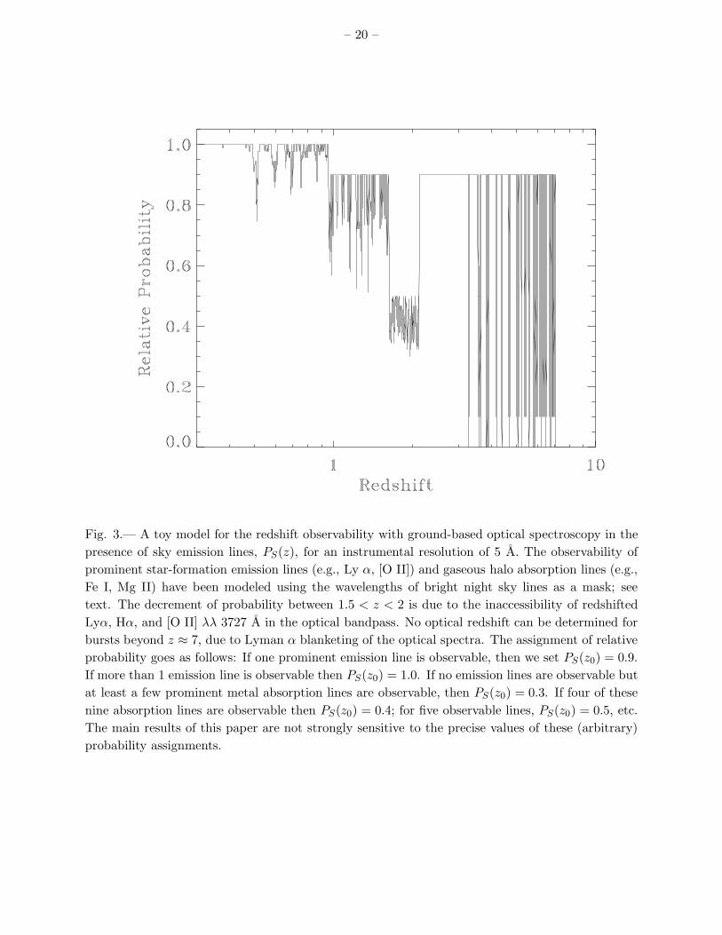
Fig. 3.— A toy model for the redshift observability with ground-based optical spectroscopy in thepresence of sky emission lines, PS(z), for an instrumental resolution of 5 A. The observability ofprominent star-formation emission lines (e.g., Ly α, [O II]) and gaseous halo absorption lines (e.g.,Fe I, Mg II) have been modeled using the wavelengths of bright night sky lines as a mask; seetext. The decrement of probability between 1.5 < z < 2 is due to the inaccessibility of redshiftedLyα, Hα, and [O II] λλ 3727 A in the optical bandpass. No optical redshift can be determined forbursts beyond z ≈ 7, due to Lyman α blanketing of the optical spectra. The assignment of relativeprobability goes as follows: If one prominent emission line is observable, then we set PS(z0) = 0.9.If more than 1 emission line is observable then PS(z0) = 1.0. If no emission lines are observable butat least a few prominent metal absorption lines are observable, then PS(z0) = 0.3. If four of thesenine absorption lines are observable then PS(z0) = 0.4; for five observable lines, PS(z0) = 0.5, etc.The main results of this paper are not strongly sensitive to the precise values of these (arbitrary)probability assignments.

– 21 –

Fig. 4.— A model distribution, P (z), of the relative probability for GRB redshift discovery usingground-based optical spectroscopy. The model is shown with low resolution for clarity. The overallshape is determined by the rate density, PG(z), constructed assuming that the GRB rate shouldfollow the Madau star-formation rate (SF1). Beyond redshift of z = 1 we assume that the relativedetectability of emission features in GRB hosts, drop as the inverse square of the luminosity distance(L = −2). The uncertainty in the precise value of L (and hence PL(z)) is also confounded by anuncertainty in the correct form of the rate density. The toy model for the redshift observabilitydue to sky-lines is shown in Figure 3. The observed redshifts are noted as vertical lines abovethe distribution. A machine-readable data file of the high resolution version of this model may beobtained from the author by request.

– 22 –

100 1000|∆v| (km/s)

0

20

40

60

80P

erce

nt G

RB

s w

ithin

|∆v|

of a

noth

er 100 Burst Sample

50 Burst Sample

26 Burst Sample P=0.

01P=

0.05

Fig. 5.— Thresholds for the detection of significant small-scale clustering as a function of GRBredshift sample size. Based upon the Monte Carlo simulation (with SF1), the curves show theobserved percentage of bursts required to be close to another burst as a function of velocity differencefor 95% and 99% confidence. For instance in a sample of 100 ground-based optical redshifts, 66bursts must lie within 1000 km/s of another burst (i.e., 33 close pairs) to be considered a statisticallysignificant excess. Note that for all samples sizes the percent requirements are similar for smallvelocity offsets, but diverge at large velocity offsets: with more bursts, the redshift density increases,so random pairing becomes more likely.

– 23 –

Table 1. Measured and corrected GRB redshifts

Burst Pos. (J2000) θCMB v,proj redshift redshift z zlhf Ref.Name α/δ km s−1 type lines

011121 11:34:30.4-76:01:41

69.1 130.0 em [O II], Hβ, [O III], He

I, Hα

0.362(1) 0.363(1) 1

990712 22:31:53.1-73:24:28

99.4 -59.4 em/abs [O II], [Ne III], Hα,

Hβ, [O III]

0.4331(2) 0.4328(2) 2

010921 22:55:59.9+40:55:53

145.8 -302.0 em [O II], Hβ, [O III], Hα 0.4509(4) 0.4494(4) 3

020405 13:58:3.1-31:22:22

45.6 255.5 em [O II], [Ne III], Hβ,

Hγ, [O III]

0.68986(4) 0.69130(8) 4

970228 05:01:46.7+11:46:54

94.1 -26.3 em [O II], [Ne III] 0.6950(3) 0.6949(3) 5

991208 16:33:53.5+46:27:21

88.4 10.2 em [O II], [O III] 0.7055(5) 0.7056(5) 6

970508 06:53:49.5+79:16:20

92.3 -14.7 em/abs [O II], [Ne III] 0.8349(3) 0.8348(3) 7

990705 05:09:54.5-72:07:53

83.6 40.6 em [O II] 0.8424(2) 0.8426(2) 8

000210 01:59:15.6-40:39:33

119.0 -176.8 em [O II] 0.8463(2) 0.8452(2) 9

970828 18:08:34.2+59:18:52

103.1 -82.5 em [O II], [Ne III] 0.9578(1) 0.9573(1) 10

980703 23:59:6.7+08:35:07

168.4 -357.6 em/abs [O II], Hδ, Hβ, Hγ,

[O III]

0.9662(2) 0.9639(2) 11

991216 05:09:31.2+11:17:07

92.2 -14.0 em/abs [O II], [Ne III] 1.02(2) 1.02(1) 12

000911 02:18:33.2+07:45:48

134.0 -253.5 em [O II] 1.0585(1) 1.0568(1) 13

980613 10:17:57.6+71:27:26

78.9 70.0 em [O II], [Ne III] 1.0969(2) 1.0974(2) 14

000418 12:25:19.3+20:06:11

32.4 308.2 em [O II], He I, [Ne III] 1.1181(1) 1.1203(1) 15

020813 19:46:41.9-19:36:05

122.7 -197.3 abs Si II, C IV, Fe II,

Al II, Al III, Mg I,

Mg II, Mn II

1.254(2) 1.253(2) 16

990506 11:54:50.1-26:40:35

22.1 338.2 em [O II] (resolved) 1.306576(42) 1.309180(135) 15

010222 14:52:12.6+43:01:06

70.4 122.4 abs Si II, C IV, Fe II,

Al II, Sn II, Mg I,

Mg II, Mn II

1.4768(2) 1.4778(2) 17

990123 15:25:30.3+44:45:59

76.5 85.1 abs Al III, Zn II, Cr II,

Zn II, Fe II, Mg II, Mg

I

1.6004(8) 1.6011(8) 18

990510 13:38:7.7-80:29:49

75.4 91.9 abs Al III, Cr II, Fe II, Mg

II, Mg I

1.6187(15) 1.6195(15) 2

000301C 16:20:18.6+29:26:36

82.1 50.1 em/abs Fe II, Mg II, O I,

C II, Si IV, Si II, C IV,

Fe II, Al II

2.0335(3) 2.0340(3) 19

000926 17:04:9.8+51:47:11

94.1 -26.2 abs Si II, C IV, Al II,

Si II, Al III, Zn II,

Fe II, Mg II, Mg I

2.0369(6) 2.0366(7) 20

011211 11:15:18.0-21:56:56

15.0 352.6 abs Si II, Si IV, Cr II, Cr

II, Si II, C IV, Al II,

Fe III

2.140(1) 2.144(1) 21

021004 00:26:54.7 158.4 -339.4 em Lyα 2.332(1) 2.328(1) 22

– 24 –

Table 2. Nearest GRB neighbors in redshift and velocity space

Burst zlhf Nearest ∆Θ |∆z| |∆v|Name Burst Name km s−1

GRB 011121 0.363(1) GRB 990712 30.3 0.070(1) 15053 ± 223GRB 990712 0.4328(2) GRB 010921 114.4 0.0166(4) 3457 ± 93GRB 010921 0.4494(4) GRB 990712 114.4 0.0166(4) 3457 ± 93GRB 020405 0.69130(8) GRB 970228 133.4 0.0036(3) 628 ± 55GRB 970228 0.6949(3) GRB 020405 133.4 0.0036(3) 628 ± 55GRB 991208 0.7056(5) GRB 970228 121.4 0.0107(5) 1887 ± 102GRB 970508 0.8348(3) GRB 990705 152.1 0.0078(3) 1278 ± 59GRB 990705 0.8426(2) GRB 000210 39.0 0.0026(2) 416 ± 47GRB 000210 0.8452(2) GRB 990705 39.0 0.0026(2) 416 ± 47GRB 970828 0.9573(1) GRB 980703 81.4 0.0066(2) 1008 ± 38GRB 980703 0.9639(2) GRB 970828 81.4 0.0066(2) 1008 ± 38GRB 991216 1.02(1) GRB 000911 42.3 0.04(1) 5419 ± 2967GRB 000911 1.0568(1) GRB 991216 42.3 0.04(1) 5419 ± 2967GRB 980613 1.0974(2) GRB 000418 54.6 0.0229(2) 3253 ± 35GRB 000418 1.1203(1) GRB 980613 54.6 0.0229(2) 3253 ± 35GRB 020813 1.253(2) GRB 990506 104.1 0.057(2) 7446 ± 266GRB 990506 1.309180(135) GRB 020813 104.1 0.057(2) 7446 ± 266GRB 010222 1.4778(2) GRB 990123 6.2 0.1233(8) 14550 ± 95GRB 990123 1.6011(8) GRB 990510 126.2 0.0184(17) 2109 ± 195GRB 990510 1.6195(15) GRB 990123 126.2 0.0184(17) 2109 ± 195GRB 000301C 2.0340(3) GRB 000926 23.8 0.0026(7) 259 ± 75GRB 000926 2.0366(7) GRB 000301C 23.8 0.0026(7) 259 ± 75GRB 011211 2.144(1) GRB 000926 105.4 0.107(1) 10383 ± 119GRB 021004 2.328(1) GRB 011211 163.0 0.185(1) 17082 ± 132GRB 971214 3.42(1) GRB 000131 134.1 1.09(1) 65197 ± 654GRB 000131 4.513(2) GRB 971214 134.1 1.09(1) 65197 ± 654

– 25 –

Table 3. Testing the Significance of the Observed Small-scale Structure

|∆v| # GRBs paired Prob. (Observed|Simulation, L = −2) Simple Prob.km s−1 ≤ |∆v| PG(z) ∝ SF1 ∝ SF2 ∝ SF3

259 2 0.530 0.471 0.438 0.408416 4 0.303 0.247 0.215 0.252628 6 0.206 0.145 0.120 0.1911008 8 0.187 0.126 0.096 0.1711278 9 0.192 0.120 0.088 0.1601997 10 0.402 0.275 0.213 0.1102109 12 0.225 0.133 0.093 0.0993253 14 0.373 0.222 0.159 0.0343457 16 0.199 0.092 0.060 0.0265419 18 0.364 0.199 0.135 0.0027446 20 0.401 0.230 0.165 6e-5

Note. — Columns (3)–(6) give the probability estimates of observing, byrandom chance, at least the observed number of GRBs (column 2) that arepaired with another within a velocity of |∆v| (column 1). Columns (3)–(5) givethe results from the Monte Carlo simulations described in the text for differentfunctional forms of the universal star-formation rate. The last column givesthe simplistic probability calculation of observing exactly the number of pairsassuming uniform selection in velocity space (equation 4 with k = col. [2]/2).The approximation breaks down for large velocities because the probabilitiesof observing more than the given number of bursts becomes non-negligible andrelativistic velocity subtraction is not taken in to account.

100 1000|∆v| (km/s)

0

20

40

60

80

Per

cent

GR

Bs

with

in |∆

v| o

f ano

ther 100 Burst Sample

50 Burst Sample

26 Burst Sample P=0.

01P=

0.05