On the Optimal Labor Income Share
52
On the Optimal Labor Income Share ∗ Jakub Growiec, a Peter McAdam, b and Jakub Mu´ ck a a SGH Warsaw School of Economics and Narodowy Bank Polski b European Central Bank Labor’s income share has attracted interest reflecting its decline. But, from an efficiency standpoint, can we say what share would hold in the social optimum? We address this ques- tion using a microfounded endogenous growth model calibrated on U.S. data. In our baseline case the socially optimal labor share is 17 percent (11 percentage points) above the decentral- ized (historical) equilibrium. This wedge reflects the presence of externalities in R&D in the decentralized equilibrium, whose importance is conditioned by the degree of factor substitutabil- ity. We also study the dependence of both long-run growth equilibriums on different model parameterizations and relate our results to Piketty’s “Laws of Capitalism.” JEL Codes: O33, O41. 1. Introduction Although interest in labor’s share of income has a long tradition in economics, current interest has crystallized around its apparent fall in recent decades across many countries. 1 Much of the public discussion suggests that the primary reason to be concerned with ∗ We thank two anonymous referees and the editor Keith Kuester for valu- able comments, as well as those of numerous seminar and workshop partici- pants. We also gratefully acknowledge financial support from the Polish National Science Center (Narodowe Centrum Nauki) under the grant Opus 14 No. 2017/27/B/HS4/00189. Jakub Mu´ ck also gives thanks for financial support from the Foundation for Polish Science within the START fellowship. The opinions expressed in this paper are those of the authors and do not necessarily reflect views of the European Central Bank, Narodowy Bank Polski, or the Eurosystem. Corresponding author (McAdam) e-mail: [email protected]. 1 The scope of economic interest in the labor share is extremely diverse—aside from the conventional political economy, inequality, and growth literatures, the labor share is an important consideration in inflation modeling (Gal´ ı and Gertler 1999; McAdam and Willman 2004) and the consequence of firm market power, de Loecker, Eeckhout, and Unger (2020). 291
Transcript of On the Optimal Labor Income Share

On the Optimal Labor Income Share∗
Jakub Growiec,a Peter McAdam,b and Jakub Mucka
aSGH Warsaw School of Economics and Narodowy Bank PolskibEuropean Central Bank
Labor’s income share has attracted interest reflecting itsdecline. But, from an efficiency standpoint, can we say whatshare would hold in the social optimum? We address this ques-tion using a microfounded endogenous growth model calibratedon U.S. data. In our baseline case the socially optimal laborshare is 17 percent (11 percentage points) above the decentral-ized (historical) equilibrium. This wedge reflects the presenceof externalities in R&D in the decentralized equilibrium, whoseimportance is conditioned by the degree of factor substitutabil-ity. We also study the dependence of both long-run growthequilibriums on different model parameterizations and relateour results to Piketty’s “Laws of Capitalism.”
JEL Codes: O33, O41.
1. Introduction
Although interest in labor’s share of income has a long traditionin economics, current interest has crystallized around its apparentfall in recent decades across many countries.1 Much of the publicdiscussion suggests that the primary reason to be concerned with
∗We thank two anonymous referees and the editor Keith Kuester for valu-able comments, as well as those of numerous seminar and workshop partici-pants. We also gratefully acknowledge financial support from the Polish NationalScience Center (Narodowe Centrum Nauki) under the grant Opus 14 No.2017/27/B/HS4/00189. Jakub Muck also gives thanks for financial support fromthe Foundation for Polish Science within the START fellowship. The opinionsexpressed in this paper are those of the authors and do not necessarily reflectviews of the European Central Bank, Narodowy Bank Polski, or the Eurosystem.Corresponding author (McAdam) e-mail: [email protected].
1The scope of economic interest in the labor share is extremely diverse—asidefrom the conventional political economy, inequality, and growth literatures, thelabor share is an important consideration in inflation modeling (Galı and Gertler1999; McAdam and Willman 2004) and the consequence of firm market power,de Loecker, Eeckhout, and Unger (2020).
291
292 International Journal of Central Banking October 2021
a low labor income share is wealth inequality. That may be a validconcern. The current paper however provides another rationale forinterest in the labor share. We demonstrate that even in a repre-sentative household model (in which wealth inequality is absent bydefinition), the level of the labor share determines whether the econ-omy is allocating its resources efficiently. Thus, we can say that thelabor share may be too low (or high)—even without distributionalconcerns.
Remarkably, there appears to be no investigation of this issuein the literature. This contrasts with equivalent discussions in thegrowth literature: since Ramsey (1928), the question of whether adecentralized economy saves “too little” is fundamental (e.g., de LaGrandville 2012). Likewise, in terms of production, modern endoge-nous growth theory typically suggests that the presence of variousdistortions implies that the economy produces less output and lessresearch and development (R&D) relative to the first-best allocation(the “social optimum”) (e.g., Jones and Williams 2000; Alvarez-Pelaez and Groth 2005). These distortions include monopoly powerand markups plus the existence of technological externalities. Theirpresence can mean that individual firms have weak incentives towork to their fullest capacity, or indeed to invest and innovate, ifnot all of the benefits accrue to them.
But what of the labor share of income? Does, for example, “toolittle” output in the decentralized economy translate into a laborshare that is also somehow too low? Ex ante, it is by no means obvi-ous. Given widespread interest in the labor share, this constitutes animportant gap in our knowledge, which we seek to address.2 In thecontext of a microfounded endogenous growth model calibrated onU.S. data, with labor- and capital-augmenting technical change inthe aggregate production function, we find that in our baseline casethe socially optimal labor share is markedly above the decentral-ized equilibrium. The decentralized labor share, in other words, istoo low.
The key channels underlying that result are the following. First,the social planner saves more and thus has more physical capital in
2Note, we not only study the implications for the labor share but also thegrowth rate, employment in the research sector, consumption, capital accumula-tion, etc.
Vol. 17 No. 4 On the Optimal Labor Income Share 293
the long run. This is because the social planner takes into accountthe social rather than purely private return on production capital,and because the planner is able to internalize the positive returnsto capital used in R&D. This abundance of capital makes laborrelatively scarce. If, and only if, both factors have a substitutionelasticity in production below one (i.e., are gross complements), thiscapital abundance pushes the labor share up.
Second, in comparison with the decentralized allocation, thesocial planner tends to allocate relatively more labor to the R&Dsectors and less to the (final good) production sector. Because labor-augmenting R&D is the ultimate source of per capita growth, thisincreases the long-run growth rate. Yet, even though the social plan-ner increases labor-augmenting R&D relative to the decentralizedallocation, it increases capital-augmenting R&D even more. Theratio of capital- to labor-augmenting R&D is always higher in thesocial planner allocation. This effect increases unit productivity ofcapital in the steady state, augmenting both production and R&Dsectors and feeding back once again to the steady-state growth rateand the labor share.
Another appealing aspect of our framework is that it can pro-vide new convincing results on one important strand of the literatureon the labor share, namely Piketty’s “Laws of Capitalism” (Piketty2014). These predict that the capital-output ratio and the capitalincome share should increase whenever the pace of economic growthdeclines. We say “convincing results” because in our setup all rel-evant variables (factor accumulation and factor intensity, growth,technological progress, marginal product of capital and thus theinterest rate, etc.) are endogenous and modeled in a sufficiently flex-ible manner. Our analysis underscores that Piketty’s laws shouldnot be interpreted causally, but rather as correlations generated bychanges in deeper characteristics of the economy. Crucially, though,in fact these correlations are not guaranteed to hold at all. Forexample, we find that increases in factor substitutability are able toraise the capital-output ratio, the capital income share, and the eco-nomic growth rate, thus simultaneously violating both of Piketty’slaws.
Finally we demonstrate that, through the lens of our model, afluctuating labor share would not in itself necessarily be a sign ofinefficiency. Rather, the planner’s solution shows that volatility in

294 International Journal of Central Banking October 2021
Figure 1. Historical Labor Share: United States(1899–2010) and France (1897–2010)
Notes: The U.S. data are taken from Piketty and Zucman (2014) over the sam-ple 1929–2010; prior to 1929 the labor share is extrapolated using the databaseby Groth and Madsen (2016), which provides compensation of employees andvalue-added data starting in 1898 based on historical source provided by Liesner(1989). The French data are also taken from Piketty and Zucman (2014). Thedashed line is the level of the labor income share and the solid line is a sim-ple moving-average process approximating its trend characteristics: 1/10
∑4j=−5,
lst−j where lst is the labor share. See also Charpe, Bridji, and McAdam (2020)for a discussion and analysis of the properties of historical labor share measures.
this share is a natural outcome. Indeed, we know from historicalsources such as Piketty and Zucman (2014) that labor incomeshares, even over long horizons (e.g., above 100 years), can fluc-tuate considerably (see figure 1 for the United States and France;see also Charpe, Bridji, and McAdam 2020).3 By comparison, canwe describe the decentralized labor share as being characterized byexcessive volatility? The reasons an optimal allocation would pro-duce oscillations, too, relate to the fact that there is an entrenchedtension between capital- and labor-augmenting technologies. Labor-augmenting developments generate economic growth but also makecapital relatively scarce, necessitating a reallocation of resourcestowards capital to overcome this scarcity. By the same token,
3Both aspects matter for any normative discussion on the labor share. Forinstance, if the labor share is falling yet still above its “optimal” level (or fluctu-ating around it), then, arguably, this might be interpreted passively, as a man-ifestation of recognized fluctuations in factor shares (e.g., Muck, McAdam, andGrowiec 2018). Indeed, given that long and persistent fluctuations in the laborshare are observed in practice, we might also wonder whether such fluctuationsare socially optimal.

Vol. 17 No. 4 On the Optimal Labor Income Share 295
capital-augmenting developments make labor relatively scarce andtrigger the opposite reallocation.
The paper is organized as follows. Section 2 describes the model(also contained in Growiec, McAdam, and Muck 2018). This is a non-scale model of endogenous growth with two R&D sectors, giving riseto capital- as well as labor-augmenting innovations, drawing fromthe seminal contributions of Romer (1990) and Acemoglu (2003).4
The model economy uses the Dixit-Stiglitz monopolistic competi-tion setup and the increasing variety framework of the R&D sectors.Two R&D sectors are included to enable an endogenous determi-nation of factor shares. Both the social planner and decentralizedallocations are solved for and compared. We see that the presenceof markups arising from imperfect competition (and market power)and technological and R&D externalities, are the key reasons whythe decentralized allocation produces relatively lower output growthand labor share.
Section 3 calibrates the model to U.S. data. We assume that arange of long-run averages from U.S. data (evaluated over 1929–2015) correspond to the decentralized balanced growth path (BGP)of the model. Around this central calibration, though, we extensivelyexamine robustness of our result to alternative parameterizations.
Thereafter, in section 4 we solve the BGP of each allocation (i.e.,decentralized and first best) and compare them. We list the chan-nels and assumptions underlying the differences between both alloca-tions. We find that—assuming that factors are gross complements inproduction—the decentralized labor share is indeed socially subopti-mal. The difference, moreover, is large: about 17 percent (11 percent-age points). We describe the mechanisms which underlie this wedge.For robustness, we also consider production characterized by Cobb-Douglas as well as gross substitutes. In the latter case, and almostonly in that case, the socially optimal labor share falls below thedecentralized one. However, already for σ = 1.25, which constitutesa mild degree of gross substitutability, its value is counterfactually
4The term “scale effect” states that an increase in an economy’s labor endow-ment leads to a higher real growth rate. This relation arises from the (counter-factual) assumption that growth is proportional to the number of R&D workers(Jones 1995).
296 International Journal of Central Banking October 2021
low (at around 0.5) and also associated with counterfactually highper capita growth rates.5
In section 5 we also study the dependence of both long-rungrowth equilibriums on model parameters and relate our resultsto Piketty’s “Laws of Capitalism.” We also consider the dynamicproperties of the model around the balanced growth path (bothin the decentralized and optimal allocation) in terms of oscillatorydynamics. Section 6 concludes. Additional material is found in theappendixes.
Finally, note that while making a first attempt at a new researchquestion, we abstract from several issues. First, to repeat a remarkmade earlier, our concern is not about inequality among heteroge-neous agents; there are many papers on this topic. Indeed, althoughthe labor share and inequality are clearly related, they are by nomeans interchangeable (Atkinson, Piketty, and Saez 2011); an econ-omy may well exhibit a socially optimal factor income division yetstill be characterized by considerable inequality—as, for example,if there are different skill characteristics in the labor force (andthus appreciable wage dispersion), asymmetric corporate or unioninsider power, or if there is financial repression and rent seeking,etc. Indeed, one can draw an analogy with Ramsey (1928)—whoseconcern lay with the level of the socially optimal aggregate sav-ings rate, not how savings behavior is distributed across economicagents (such as by wealth, age percentiles, etc.). Our concern there-fore is somewhat more straightforward—namely, how would a socialplanner choose functional income shares. And, would that share berealistic6 in terms of its central value (relative to the decentralizedoptimum) and its volatility (again compared with the decentralizedoptimum and historical averages). Second, we do not discuss policydesigns able to alleviate the discrepancy between the decentralizedallocation and the social optimum, nor the dynamics with which
5It may be, as Piketty and Zucman (2014) argue, that one might expect ahigher elasticity of substitution in “high-tech” economies where there are lots ofalternative uses and forms for capital.
6By way of realism, consider another “optimal” rule in growth theory: namelythe golden rule savings ratio which in standard form equates the optimal savingsrate with the capital income share (which is usually around 30 percent); see dela Grandville (2012). With the exception of some Asian economies and for someparticular periods, such values are highly counterfactual.
Vol. 17 No. 4 On the Optimal Labor Income Share 297
they could be introduced.7 Our results are obtained by compar-ing long-run equilibriums of two entirely separate model economies(decentralized and first-best allocation). Therefore we are silent onthe possible evolution of the labor share along the transition pathfollowing the introduction of policy measures able to shift the decen-tralized allocation towards the first best. In consequence, we cannotsay (i) if the labor share should rise or fall in the short to mediumrun, and (ii) how long the transition to the optimal labor shareshould take.
2. Model
The framework is a generalization of Acemoglu (2003) with capital-and labor-augmenting R&D, building on the earlier induced inno-vation literature from Kennedy (1964) onwards as well as generalinnovation in monopolistic competition and growth literatures (e.g.,Dixit and Stiglitz 1977, Romer 1990, and Jones 1999).
By “generalization” we mean that we relax a number of featuresto make our conclusions more applicable to the studied question,as well as to correct for some counterfactual features (such as theaforementioned scale effects). Formally, (i) our model is non-scale:both R&D functions are specified in terms of percentages of pop-ulation employed in either R&D sector; (ii) we also assume R&Dworkers are drawn from the same pool as production workers;8 (iii)we assume more general R&D technologies which allow for mutualspillovers between both R&D sectors (cf. Li 2000) and for concavityin capital-augmenting technical change; (iv) in contrast to Acemoglu(2003), the BGP growth rate in our model depends on preferencesvia employment in production and R&D—the tradeoff is due todrawing researchers from the same employment pool as production
7Interestingly, Atkinson (2015) lists a number of proposals for reducinginequality trends, the first of which is that “the direction of technical changeshould be an explicit concern of policy-makers.”
8Acemoglu (2003) assumes that labor supply in the production sector is inelas-tic and R&D is carried out by a separate group of “scientists” who cannot engagein production labor. Our assumption affects the tension between both R&Dsectors by providing R&D workers with a third option, the production sector.

298 International Journal of Central Banking October 2021
workers (a tradeoff not present in his model); and (v) we use normal-ized constant elasticity of substitution (CES) production functions9
which, importantly, ensures valid comparative static comparisons inthe elasticity of factor substitution. To start matters off, we considerthe simpler case of the social planner allocation.10
2.1 The Social Planner’s Problem
The social planner maximizes the representative household’s utilityfrom discounted consumption, c, given standard constant relativerisk aversion (CRRA) preferences, (1).
max∫ ∞
0
c1−γ − 11 − γ
e−(ρ−n)tdt, (1)
where γ > 0 is the inverse of the intertemporal elasticity of sub-stitution, ρ > 0 is the rate of time preference, and n > 0 is the(exogenous) growth rate of the labor supply.
The maximization is subject to the budget constraint (2) (i.e.,the equation of motion of the aggregate per capita capital stock k),the “normalized” production function (3), the two R&D technologies(4)–(5), and the labor market clearing condition (6):11
k = y − c − (δ + n)k − ζa, (2)
y = y0
(π0
(λb
k
k0
)ξ
+ (1 − π0)(
λa
λa0
Y
Y 0
)ξ)1/ξ
, (3)
9Normalization essentially implies representing the production relations inconsistent index number form. Its parameters then have a direct economic inter-pretation. Otherwise, the parameters can be shown to be scale dependent (i.e.,a circular function of σ itself, as well as a function of the implicit normalizationpoints). Subscript 0’s denote the specific normalization points: geometric (arith-metic) averages for non-stationary (stationary) variables. See de la Grandville(1989), Klump and de la Grandville (2000), and Klump and Preissler (2000) forthe seminal theoretical contributions. In our case, normalization is essentiallyimportant, since comparative statics on production function parameters are akey concern.
10It is simpler because, solving under the social optimum, we can imposesymmetry directly and deal in terms of aggregates; see Benassy (1998).
11There are three control (c, �a, �b) and three state (k, λa, λb) variables in thisoptimization problem.
Vol. 17 No. 4 On the Optimal Labor Income Share 299
λa = A(λaλφ
b xηaνaa
), (4)
λb = B(λ1−ω
b xηbνb
b
)− dλb, (5)
1 = a + b + Y . (6)
In (2) and (3), y = Y/L and k = K/L (i.e., output and capitalper capita), where L is total employment and a and b are the shares(or “research intensity”) employed in labor- and capital-augmentingR&D, respectively (and, respectively, generating increases in λa andλb). The remaining fraction of population Y is employed in pro-duction. We assume that capital augmentation is subject to gradualdecay at rate d > 0, which mirrors susceptibility to obsolescenceand embodied character of capital-augmenting technologies; Solow(1960). This assumption is critical for the asymptotic constancy ofunit capital productivity λb in the model, and thus for the existenceof a BGP with purely labor-augmenting technical change.
The term π denotes the capital income share, and ξ = σ−1σ , where
σ ∈ [0,∞) is the elasticity of substitution between capital and labor.This parameter, important in many contexts,12 turns out also to becritical in our analysis with the distinction as to whether factorsare gross complements, i.e., σ < 1, or gross substitutes, σ > 1, inproduction.
Factor-augmenting innovations are created endogenously by therespective R&D sectors (Acemoglu 2003), increasing the underlyingparameters λa, λb, as in (4) and (5). Parameters A and B capturethe unit productivity of the labor- and capital-augmenting R&Dprocess, respectively; φ captures the spillover from capital- to labor-augmenting R&D;13 and ω measures the degree of decreasing returns
12CES function (3) nests the linear, Cobb-Douglas, and Leontief forms, respec-tively, when ξ = 1, 0, −∞. The value of the elasticity of factor substitution hasbeen shown to be a key parameter in many economic fields: e.g., the gains fromtrade (Saam 2008); the strength of extensive growth (de La Grandville 2016);multiple growth equilibriums, development traps, and indeterminacy (Azariadis1996; Klump 2002; Kaas and von Thadden 2003; Guo and Lansing 2009); theresponse of investment and labor demand to various policy changes and shocks(Rowthorn 1999); etc.
13We assume φ > 0, indicating that more efficient use of physical capital alsoincreases the productivity of labor-augmenting R&D. Observe, there are mutualspillovers between both R&D sectors, with no prior restriction on their strength:λa = Aλ1−ηa
a λφ+ηab kηa�νa
a and λb = Bλ−ηba λ
1−ω+ηbb kηb�
νbb − dλb.
300 International Journal of Central Banking October 2021
to scale in capital-augmenting R&D. By assuming ω ∈ (0, 1) we allowfor the “standing on shoulders” effect in capital-augmenting R&D,albeit we limit its scope insofar as it is less than proportional to theexisting technology stock (Jones 1995).
The term x ≡ λbkλa
captures the technology-corrected degree ofcapital augmentation of the workplace. This term represents posi-tive spillovers from capital intensity in the R&D sector and will beconstant along the BGP. The long-term endogenous growth engine islocated in the linear labor-augmenting R&D equation. To fulfill therequirement of the existence of a BGP along which the growth ratesof λa and λb are constant, we assume that ηbφ + ηaω �= 0.14 Notethat the above parameterization of R&D equations, with six freeparameters in equations (4)–(5), is the most general one possibleunder the requirement of existence of a BGP with purely labor-augmenting technical change (Uzawa 1961; Jones 1999; Acemoglu2003; Growiec 2007).
The last term in (2) captures a negative externality that arisesfrom implementing new labor-augmenting technologies, with ζ ≥ 0.Motivated by Leon-Ledesma and Satchi (2019), we allow for a non-negative cost of adopting new labor-augmenting technologies: sinceworkers (as opposed to machines) need to develop skills compatiblewith each new technology, it is assumed that there is a capital costof such technology shifts (potentially representing training costs,learning-by-doing, etc.). We posit that new capital investments are
diminished by ζa, where a = gλa
(ππ0
)1/α
, g being the economicgrowth rate (Growiec, McAdam, and Muck 2018). For analyticalsimplicity we consider these costs exogenous to the firms.
Finally, R&D activity may be subject to duplication externali-ties; the greater the number of researchers searching for new ideas,the more likely is duplication. Thus research effort may be charac-terized by diminishing returns; Kortum (1993). This is captured byparameters νa, νb ∈ (0, 1]: the higher is ν, the lower the extent ofduplication.15
14All our qualitative results also go through for the special case ηa = ηb = 0,which fully excludes capital spillovers in R&D. The current inequality conditionis not required in such cases.
15Observe that switching off all externalities and spillovers in (4)–(5) by settingd = ω = ηa = ηb = 0 and νa = νb = 1 retrieves the original specification of R&D

Vol. 17 No. 4 On the Optimal Labor Income Share 301
Variables with subscript 0 (π0, y0, k0, λa0, Y 0) are CES normal-ization constants.
2.2 Decentralized Allocation
The construction of the decentralized allocation draws from Romer(1990), Acemoglu (2003), and Jones (2005). It has been also pre-sented in Growiec, McAdam, and Muck (2018). We use the Dixitand Stiglitz (1977) monopolistic competition setup and the increas-ing variety framework of the R&D sector. The general equilibriumis obtained as an outcome of the interplay between households;final goods producers; aggregators of bundles of capital- and labor-intensive intermediate goods; monopolistically competitive produc-ers of differentiated capital- and labor-intensive intermediate goods;and competitive capital- and labor-augmenting R&D firms.
2.2.1 Households
Analogous to the social planner’s allocation, we again assume thatthe representative household maximizes discounted CRRA utility:
max∫ ∞
0
c1−γ − 11 − γ
e−(ρ−n)tdt
subject to the budget constraint:
v = (r − δ − n)v + w − c, (7)
where v = V/L is the household’s per capita holding of assets,V = K + paλa + pbλb. The representative household is the owner ofall capital and also holds the shares of monopolistic producers of dif-ferentiated capital- and labor-intensive intermediate goods (pricedpa and pb, respectively). Capital is rented at a net market rental rate
in Acemoglu (2003). Moreover, compared with models which use Cobb-Douglasproduction, equation (5) is akin to Jones’s (1995) formulation of the R&D sector,generalized by adding obsolescence and positive spillovers from capital intensity.Thus, setting d = ηb = 0 retrieves Jones’s original specification. And (4) is thesame as in Romer (1990) but scale free (it features �b instead of �b · L), witha positive spillover from capital intensity and a direct spillover from λb; settingφ = ηa = 0 retrieves the scale-free version of Romer (1990), cf. Jones (1999).

302 International Journal of Central Banking October 2021
equal to the gross rental rate after depreciation: r − δ. In turn, w isthe market wage rate. Solving the household’s optimization problemyields the familiar Euler equation:
c =r − δ − ρ
γ, (8)
where c = c/c is the per capita growth rate (“hats” denote growthrates).
2.2.2 Final Goods Producers
The role of final goods producers is to generate the output of finalgoods (which are then either consumed by the representative house-hold or saved and invested, leading to physical capital accumula-tion), taking bundles of capital- and labor-intensive intermediategoods (YK , YL) as inputs. They operate in a perfectly competitiveenvironment, where both bundles are remunerated at market ratespK and pL, respectively.
The final goods producers operate a normalized CES technology:
Y = Y0
(π0
(YK
YK0
)ξ
+ (1 − π0)(
YL
YL0
)ξ) 1
ξ
. (9)
The optimality condition implies that final goods producers’ demandfor capital- and labor-intensive intermediate goods bundles satisfies
pK
pL=
π
1 − π
YL
YK, (10)
where π = π0
(YK
YK0
Y0Y
)ξ
is the elasticity of final output with respectto YK (in equilibrium it will be equal to the labor share).
2.2.3 Aggregators of Capital- and Labor-IntensiveIntermediate Goods
There are two symmetric sectors whose role is to aggregate the dif-ferentiated (capital- or labor-intensive) goods into the bundles YK
and YL demanded by final goods producers. It is assumed that the

Vol. 17 No. 4 On the Optimal Labor Income Share 303
differentiated goods are imperfectly substitutable (albeit gross sub-stitutes). The degree of substitutability is captured by parameterε ∈ (0, 1):
YK =
(∫ NK
0Xε
Kidi
) 1ε
. (11)
Aggregators operate in a perfectly competitive environment anddecide upon their demand for intermediate goods, the price of whichwill be set by the respective monopolistic producers (discussed in thefollowing subsection).
For capital-intensive bundles, the aggregators maximize
maxXKi
⎧⎨⎩pK
(∫ NK
0Xε
Kidi
) 1ε
−∫ NK
0pKiXKidi
⎫⎬⎭ . (12)
There is a continuum of measure NK of capital-intensive interme-diate goods producers. Optimization implies the following demandcurve:
XKi = xK(pKi) =(
pKi
pK
) 1ε−1
Y1ε
K . (13)
Equivalent terms follow for labor-intensive intermediate goods pro-ducers.
2.2.4 Producers of Differentiated Intermediate Goods
It is assumed that each of the differentiated capital- or labor-intensive intermediate goods producers, indexed by i ∈ [0, NK ] ori ∈ [0, NL], respectively, has monopoly over its specific variety. It istherefore free to choose its preferred price pKi or pLi. These firmsoperate a simple linear technology, employing either only capital oronly labor.
For the case of capital-intensive intermediate goods producers,the production function is XKi = Ki. Capital is rented at the grossrental rate r. The optimization problem is
maxpKi
(pKiXKi − rKi) = maxpKi
(pKi − r)xK(pKi). (14)
304 International Journal of Central Banking October 2021
The optimal solution implies pKi = r/ε for all i ∈ [0, NK ]. Thisimplies symmetry across all differentiated goods: they are sold atequal prices, thus their supply is also identical, XKi = XK for all i.Market clearing implies
K =∫ NK
0Kidi =
∫ NK
0XKidi = NKXK , YK = N
1−εε
K K. (15)
The demand curve implies that the price of intermediate goodsis linked to the price of the capital-intensive bundle as in pK =pKiN
ε−1ε
K = rεN
ε−1ε
K .The labor-intensive sector follows symmetrically: XLi = LY i,
LY = Y L =∫ NL
0 LY idi, and pLi = w/ε, pL = pLiNε−1
ε
L = wε N
ε−1ε
L ,where w is the market wage rate.
Aggregating across all intermediate goods producers, we obtainthat their total profits are equal to ΠKNK = rK
(1−εε
)and
ΠLNL = wLY
(1−εε
)for capital- and labor-intensive goods, respec-
tively. Streams of profits per person in the representative house-hold are thus πK = ΠK/L and πL = ΠL/L, respectively. Hence,the total remuneration channeled to the capital-intensive sectorequals pKYK = r
εK = rK + ΠKNK , whereas the total remuner-ation channeled to the labor-intensive sector equals pLYL = w
ε LY =wLY + ΠLNL.
In equilibrium, factor shares then amount to
π = π0
(KY0
Y K0
)ξ (NK
NK0
)ξ( 1−εε )
, (16)
1 − π = (1 − π0)(
Y0LY
Y LY 0
)ξ (NL
NL0
)ξ( 1−εε )
. (17)
Incorporating all these choices into (9), and using the definitions
λb = N1−ε
ε
K and λa = N1−ε
ε
L retrieves production function (3).
2.2.5 Capital- and Labor-Augmenting R&D Firms
The role of capital- and labor-augmenting R&D firms is to pro-duce innovations which increase the variety of available differenti-ated intermediate goods, either NK or NL, and thus indirectly also
Vol. 17 No. 4 On the Optimal Labor Income Share 305
λb and λa. Patents never expire, and patent protection is perfect.R&D firms sell these patents to the representative household, whichsets up a monopoly for each new variety. Patent price, pb or pa,which reflects the discounted stream of future monopoly profits, isset at the competitive market. There is free entry to R&D.
R&D firms employ labor only: La = aL and Lb = bL work-ers are employed in the labor- and capital-augmenting R&D sector,respectively. There is also an externality from the physical capitalstock per worker, working through the capital spillover term in theR&D production function. Furthermore, the R&D firms perceivetheir production technology as linear in labor, while in fact it isconcave due to duplication externalities (Jones 1995).
Incorporating these assumptions and using the notion x ≡λbk/λa, capital-augmenting R&D firms maximize
max�b
(pbλb − wb
)= max
�b
((pbQK − w)b) , (18)
where QK = B(λ1−ω
b xηbνb−1b
)is treated by firms as an exoge-
nously given constant (Romer 1990; Jones 2005). Analogously, labor-augmenting R&D firms maximize
max�a
(paλa − wa
)= max
�a
((paQL − w)a) , (19)
where QL = A(λaλφ
b xηaνa−1a
)is treated as exogenous.
Free entry into both R&D sectors implies w = pbQK = paQL.Purchase of a patent entitles the holders to a per capita stream ofprofits equal to πK and πL, respectively. While the production of anylabor-augmenting varieties lasts forever, there is a constant rate dat which production of capital-intensive varieties becomes obsolete.This effect is external to patent holders and thus is not strategicallytaken into account when accumulating the patent stock.16
2.2.6 Equilibrium
We define the decentralized equilibrium as the collection of timepaths of all the respective quantities: c, a, b, k, λb, λa, YK , YL,
16In other words, by solving a static optimization problem, capital-augmentingR&D firms do not take the dynamic (external) obsolescence effect into account.

306 International Journal of Central Banking October 2021
{XKi}, {XLi} and prices r, w, pK , pL, {pKi}, {pLi}, pa, pb such that(i) households maximize discounted utility subject to their budgetconstraint; (ii) profit maximization is followed by final goods pro-ducers, aggregators and producers of capital- and labor-intensiveintermediate goods, and capital- and labor-augmenting R&D firms;(iii) the labor market clears: La+Lb+LY = (a+b+Y )L = L; (iv)the asset market clears: V = vL = K + paλa + pbλb, where assetshave equal returns: r − δ = πL
pa+ pa
pa= πK
pb+ pb
pb− d; and, finally,
(v), such that the aggregate capital stock satisfies K = Y − C −δK − ζaL.
2.3 Solving for the Social Planner Allocation
In this section, we first solve analytically for the BGP of the socialplanner (SP) allocation of our endogenous growth model and thenlinearize the implied dynamical system around the BGP.
2.3.1 Balanced Growth Path
Any neoclassical growth model can exhibit balanced growth only iftechnical change is purely labor augmenting or if production is Cobb-Douglas; Uzawa (1961). That condition holds here too. Hence, oncewe presume a CES production function, the analysis of dynamicconsequences of any technical change which is not purely labor aug-menting must be done outside the BGP.
Along the BGP, we obtain the following growth rate of key modelvariables:
g = λa = k = c = y = A(λ∗b)
φ (x∗)ηa (∗a)νa , (20)
where stars denote steady-state values. Hence, ultimately long-rungrowth is driven by labor-augmenting R&D. This can be explainedby the fact that labor is the only non-accumulable factor in themodel, it is complementary to capital along the aggregate produc-tion function, and the labor-augmenting R&D equation is linearwith respect to λa. The following variables are constant along theBGP: y/k, c/k, a, b, and λb (i.e., asymptotically there is no capital-augmenting technical change).
Vol. 17 No. 4 On the Optimal Labor Income Share 307
2.3.2 Euler Equations
Having set up the Hamiltonian (with co-state variables μk, μa, μb),
H(c, a, b, k, λa, λb; μk, μa, μb) =c1−γ − 1
1 − γe−(ρ−n)t
+ μk(y − c − (δ + n)k − ζa)
+ μaA(λaλφ
b xηaνaa
)+ μb
(B
(λ1−ω
b xηbνb
b
)− dλb
),
(21)
where
y = y0
(π0
(λb
k
k0
)ξ
+ (1 − π0)(
λa
λa0
1 − a − b
Y 0
)ξ)1/ξ
, (22)
computed its derivatives, and eliminated the co-state variables, aftertedious algebra the following Euler equations are obtained for theSP:17
c =1γ
(y
k
(π +
1 − π
Y
(ηaa
νa+
ηbb
νb
))− δ − ρ
), (23)
ϕ1a + ϕ2b = Q1, (24)
ϕ3a + ϕ4b = Q2, (25)
where
ϕ1 = νa − 1 − (1 − ξ)πa
Y, (26)
ϕ2 = −(1 − ξ)πb
Y, (27)
17A sufficient condition for all transversality conditions to be satisfied in thesocial optimum (as well as in the decentralized equilibrium) is that (1 − γ)g +n < ρ.

308 International Journal of Central Banking October 2021
ϕ3 = −(1 − ξ)πa
Y, (28)
ϕ4 = νb − 1 − (1 − ξ)πb
Y, (29)
and
Q1 = −γc − ρ + n + λa
(Y νa
a+ 1 − ηa − ηb
bνa
aνb
)
− φλb + ((1 − ξ)π − ηa)x, (30)
Q2 = −γc − ρ + n + λa + λb
(π
1 − π
Y νb
b+ (φ + ηa)
νba
νab+ ηb
)
+ ((1 − ξ)π − ηb)x + d
(π
1 − π
Y νb
b+ (φ + ηa)
νba
νab−ω + ηb
).
(31)
2.3.3 Steady State and Linearization of the TransformedSystem
The above Euler equations and dynamics of state variables are thenrewritten in terms of stationary variables which are constant alongthe BGP, i.e., in coordinates: u = (c/k), a, b, x, λb, and with aux-iliary variables z = (y/k), π, g. The full steady state of the trans-formed system is listed in appendix A.1. This nonlinear systemof equations is solved numerically, yielding a steady state of thedetrended system and thus a BGP of the model in original vari-ables.18 All further analysis of the social planner allocation is basedon the (numerical) linearization of the five-dimensional dynamicalsystem of equations (23)–(25), (2), and (5), taking the BGP equality(20) as given.
2.4 Solving for the Decentralized Allocation
When solving for the decentralized allocation (DA), we broadly fol-low the steps carried out in the case of the social planner (SP)
18We do not have a formal proof of BGP uniqueness, but the large numberof numerical checks we have performed (e.g., varying initial conditions of thenumerical algorithm, modifying values of model parameters), is suggestive thatthe BGP is indeed unique and depends smoothly on model parameters.

Vol. 17 No. 4 On the Optimal Labor Income Share 309
allocation. We first solve analytically for the BGP of our endoge-nous growth model and then linearize the implied dynamical systemaround the BGP.
2.4.1 Balanced Growth Path
Along the BGP, we obtain the following growth rate of the key modelvariables:
g = k = c = y = w = pb = pLi = λa = A(λ∗b)
φ (x∗)ηa (∗a)νa . (32)
The following quantities are constant along the BGP: y/k, c/k, a, b,YK/Y, YL/Y, and λb (again, note, asymptotically, the absence ofcapital-augmenting technical change). The following prices are alsoconstant along the BGP: r, pa, pK , pL, {pKi}.
2.4.2 Euler Equations
The decentralized equilibrium is associated with the following Eulerequations describing the first-order conditions:
c =επ y
k − δ − ρ
γ, (23′)
ϕ1a + ϕ2b = Q1, (24′)
ϕ3a + ϕ4b = Q2, (25′)
where
Q1 = −επy
k+ δ + λa
Y
a− φλb + ((1 − ξ)π − ηa)x (30′)
Q2 = −επy
k+ δ + λa + (λb + d)
(π
1 − π
Y
b
)
− λb(1 − ω) − d + ((1 − ξ)π − ηb)x (31′)
and ϕ1 through ϕ4 are defined as in (26)–(29). The full steady stateof the transformed system is listed in appendix A.2. All furtheranalysis of the decentralized allocation is based on the (numerical)

310 International Journal of Central Banking October 2021
linearization of the five-dimensional dynamical system of equations(23′)–(25′), (2), and (5), taking the BGP equality (32) as given.
2.4.3 Departures from the Social Optimum
Departures of the decentralized allocation from the optimal one canbe tracked back to specific assumptions regarding the informationstructure of the decentralized allocation. In the following we try tocompare one-to-one all the differences in the equations related to thedecentralized and to social planner outcome. As we shall show, thosedifferences follow from the presence of wedges (such as markupsfrom imperfect competition) and externalities (such as duplicationexternalities from R&D investment). These differences also showin different costs and returns that exist in the social planner anddecentralized allocation.
Specifically, the points of comparison are as follows:
1. In the consumption Euler equation, comparing equations (23)with (23′), the term y
k
(π + 1−π
�Y
(ηa�a
νa+ ηb�b
νb
))is replaced by
επ yk . This is due to two effects:(a) in contrast to the social planner, markets fail to account
for the external effects of physical capital on R&Dactivity via the capital spillover terms (with respectiveelasticities ηb and ηa);
(b) ε appears in the decentralized allocation due to imper-fect competition in the labor- and capital-augmentingintermediate goods sectors.
Both effects work in the same direction and buy the socialplanner much more capital in the steady state. The savingsrate is much higher in the SP allocation, as two effects addup: (i) accounting for social instead of private returns on pro-duction capital, (ii) internalizing the positive returns to cap-ital used in R&D. Therefore in the social planner’s steadystate, there is relatively lower consumption and output perunit of capital, and greater positive capital spillover in R&D,x = λbk
λa.
This abundance of capital makes labor relatively scarce,which—if and only if both factors are gross complements

Vol. 17 No. 4 On the Optimal Labor Income Share 311
(σ < 1)—increases the labor share in the social plannerallocation relative to the decentralized equilibrium.
2. In the Euler equation for a, the term(
�Y νa
�a+ 1 − ηa − ηb
�bνa
�aνb
),
is replaced by �Y
�a. Analogously, in the Euler equation for b,
the term given by �Y νb
�b
π1−π + (1 − ω) + ηb + (φ + ηa) �aνb
�bνais
replaced by �Y
�b
π1−π . This is due to two effects:
(a) νa and νb are missing in the respective first compo-nents because markets fail to internalize the detrimen-tal R&D duplication effects;
b) the latter two components are missing because mar-kets fail to account for the positive external effects ofaccumulating knowledge on future R&D productivity.These effects are included in the shadow prices of λa
and λb in the social planner allocation but not in theirrespective market prices.
The effect (a) reduces SP’s investment in R&D, whereasthe effect (b) increases it. In our baseline calibration and itsrobustness checks, on balance the latter effect robustly pre-vails and the social planner allocates less labor to productionand more to R&D (greater a and b). Hence, this mechanismcauses the social planner to accumulate more investment inboth R&D sectors. This, given that labor-augmenting techno-logical progress is the ultimate source of growth in the model,increases the long-run growth rate.
3. In the Euler equations for a and b (equations (24), (25),(24′), and (25′)) the shadow price of physical capital c−ρ+nis replaced by its market price r − δ = επ y
k − δ, which islower because it accounts for markups arising from imperfectcompetition.
This mechanism causes the social planner to accumu-late more capital-augmenting R&D b relative to labor-augmenting R&D a. Therefore the ratio of capital- to labor-augmenting R&D employment is always higher in the socialoptimum than in the decentralized allocation. Hence, unitcapital productivity (λb) is higher in the SP steady state.This further adds to the capital spillover term x which, in

312 International Journal of Central Banking October 2021
turn, augments both R&D sectors, accelerates growth and—by making labor relatively scarce—increases the labor share.
3. Calibration of the Model
3.1 Empirical Calibration Components
The parameter calibration for the decentralized model based on mag-nitudes from historical data or empirical studies is listed in table 1.We assume that a range of long-run averages from U.S. data (1929–2015) correspond to the decentralized BGP of the model. Doing soallows us to calibrate the rates of economic and population growth,capital productivity and income share, and the consumption-to-capital ratio. Likewise, we assign CES normalization parameters tomatch U.S. long-run averages for factor income shares (we adjustthe payroll share by proprietors’ income, as in Muck, McAdam, andGrowiec 2018). This implies an average labor share of 0.67.19
Next, we turn to the elasticity of substitution between labor andcapital (σ) which is the fundamental economic parameter in ouranalysis. We calibrate factors to be gross complements, i.e., σ < 1.This choice stems from a fact that the bulk of empirical studies forthe U.S. aggregated production function document that the σ is sys-tematically below unity (Klump, McAdam, and Willman 2012).20
Most of the empirical evidence exploiting time-series variation forother countries also implies σ < 1 (McAdam and Willman 2013;Muck 2017; Knoblach and Stockl 2020).
However, the literature based predominantly on cross-countryvariation is rather inconclusive about the magnitude of σ. On onehand, several papers (Piketty and Zucman 2014; Karabarbounis andNeiman 2014) employ gross substitutes; however, the former paper
19Note that in the model, due to the inelastic labor supply and the firm profitsbeing rebated to the household, markups do not directly affect factor shares.
20For instance, Arrow et al. (1961) found an aggregate elasticity over 1909–49of 0.57 (similar to that of the more recent Antras 2004). More recently, Klump,McAdam, and Willman (2007) reported σ ≈ 0.7. The tendency towards grosscomplementarity between factors is also confirmed at the industry level (Her-rendorf, Herrington, and Valentinyi 2015; Laeven, McAdam, and Popov 2018)and firm level (Oberfield and Raval 2018). Importantly, the elasticity uncov-ered is found systematically below unity even if more flexible functional forms ofaggregate production function are considered (Growiec and Muck 2020).

Vol. 17 No. 4 On the Optimal Labor Income Share 313
Tab
le1.
Cal
ibra
ted
Par
amet
ers
(dec
entr
aliz
edal
loca
tion
)
Par
amet
erSym
bol
Val
ue
Tar
get/
Sou
rce
Inco
me
and
Pro
duct
ion
GD
Ppe
rca
pita
Gro
wth
g0.
0171
Geo
met
ric
Ave
rage
Pop
ulat
ion
Gro
wth
Rat
en
0.01
53G
eom
etri
cA
vera
geC
apit
alP
rodu
ctiv
ity
z 0,z
∗0.
3442
Geo
met
ric
Ave
rage
Con
sum
ptio
n-to
-Cap
ital
u∗
0.21
99G
eom
etri
cA
vera
geC
apit
alIn
com
eSh
are
π0,π
∗0.
3260
Ari
thm
etic
Ave
rage
Dep
reci
atio
nδ
0.06
00C
asel
li(2
005)
Fact
orSu
bsti
tuti
onPar
amet
erξ
−0.
4286
⇒σ
=0.
7,K
lum
p,M
cAda
m,an
dW
illm
an(2
007)
Pre
fere
nces
Inve
rse
Inte
rtem
pora
lγ
1.75
00B
arro
and
Sala
-i-M
arti
n(2
003)
Ela
stic
ity
ofSu
bsti
tuti
onT
ime
Pre
fere
nce
ρ0.
0200
Bar
roan
dSa
la-i-M
arti
n(2
003)
Note
s:T
his
tabl
esh
ows
the
para
met
erva
lues
that
are
used
inth
ece
ntra
lca
libra
tion
ofth
em
odel
.T
heva
lues
are
take
nfr
omhi
stor
ical
aver
ages
(192
9–20
15)
ofth
ere
leva
ntU
.S.ti
me
seri
es.
314 International Journal of Central Banking October 2021
calibrates the σ value and the latter estimates it in a cross-countrypanel context.21 On the other hand, recent studies exploiting macropanels and allowing for factor augmentation in the supply-side sys-tem approach strongly conclude in favor of gross complementarityin production (Muck 2017). Given this, we consider σ < 1 as thebenchmark, but we do examine the σ > 1 case in our robustnessexercises.
Finally, the table includes preference parameters (intertempo-ral elasticity of substitution, time preference) which are difficult toretrieve from historical data. For that reason, in our central calibra-tion we rely on values typically found in the literature.
3.2 Model-Consistent Calibration Components
Next, conditional on the values in table 1, four identities included inthe system (see appendix equations (A.9)–(A.17)) drive the calibra-tion of other parameters in a model-consistent manner: r∗, λ∗
b , x∗,and ε. Employment in final production ∗
Y is also set in a model-consistent manner (table 2).
In the absence of any other information, we agnostically assumethat the share of population 1 − ∗
Y is split equally between employ-ment in both (i.e., capital and labor) R&D sectors in the decen-tralized allocation—although notice these employment shares areendogenous in the social planner solution. For the model-consistentvalue of ∗
Y , the relevant formula leads to values close to those typ-ically considered for the non-routine cognitive occupational group(e.g., Jaimovich and Siu 2020, using Bureau of Labor Statisticsdata, show this ratio to be between 29 percent and 38 percent, over1982–2012).
For the duplication externalities, we assume νa = νb = 0.75 fol-lowing the (albeit single R&D sector) value in Jones and Williams(2000) (although, note again, we conduct extensive robustness checkson these values). The steady-state level of unit capital productivityλ∗
b is normalized to unity, and so are CES normalization parametersλa0 and λb0.
21The latter paper moreover was estimated on a single-equation non-normalizedbasis which is known to have poor estimation properties in this context (Leon-Ledesma, McAdam, and Willman 2010; Klump, McAdam, and Willman 2012).

Vol. 17 No. 4 On the Optimal Labor Income Share 315
Tab
le2.
Par
amet
eran
dSte
ady-S
tate
Var
iable
Cal
ibra
tion
Con
ditio
nal
onH
isto
rica
lA
vera
geC
alib
ration
(dec
entr
aliz
edal
loca
tion
)
Par
amet
erSym
bol
Val
ue
Tar
get/
Sou
rce
Inco
me
and
Pro
duct
ion
Net
Rea
lR
ate
ofR
etur
nr∗
−δ
0.04
99r∗
−δ
=γg
+ρ
Subs
titu
tabi
lity
betw
een
Inte
rmed
iate
Goo
dsε
0.97
93ε
=r
∗
π∗z
∗
R&
DSe
ctor
s
R&
DD
uplic
atio
nPar
amet
ers
υa
=υ
b0.
7500
Jone
san
dW
illia
ms
(200
0)Tec
hnol
ogy
Aug
men
ting
Ter
ms
λa0,λ
b0
1N
orm
aliz
edto
Uni
ty
Uni
tC
apit
alP
rodu
ctiv
ity
λ∗ b
1λ
∗ b=
λb0
z∗
z0
( π∗
π0
)1 ξ
Em
ploy
men
tSh
are
inR
&D
Sect
ors
∗ a,
∗ b0.
2033
∗ a=
∗ bfo
r∗ a
+∗ b
=1
−∗ Y
Cap
ital
–Lab
orR
atio
inE
ffici
ency
Uni
ts†
x0,x
∗61
.790
0x
∗=
x0
�∗ Y
� Y0
(1
1−π0
( z∗
z0
λb0
λ∗ b
) ξ −π0
1−π0
) −1/ξ
Note
s:T
his
tabl
esh
ows
the
para
met
eran
dst
eady
-sta
teva
riab
leva
lues
that
are
used
inth
ece
ntra
lca
libra
tion
ofth
em
odel
.T
heva
lues
are
take
nfr
omva
lues
cons
iste
ntw
ith
the
stru
ctur
eof
the
mod
elor
from
othe
rre
leva
ntst
udie
sin
the
liter
atur
e.† x
0=
λb0k0
λa0
=61
.79.

316 International Journal of Central Banking October 2021
The final step is to assign values to the remaining parame-ters, in particular the technological parameters of the R&D equa-tions. We do this by solving the four remaining equations in system(A.9)–(A.17) with respect to the remaining parameters; see tableB.1. Given this benchmark calibration, the steady state is a saddlepoint.
4. Is the Decentralized Labor Share Socially Optimal?
Given the model setup and its benchmark calibration, we can nowcome to our central question: is the decentralized labor share sociallyoptimal? In table 3, columns 1 and 2 show the decentralized allo-cation (DA) and social planner (SP) outcomes for our benchmarkcalibration; columns 3 and 4, considered later, alternatively imposeCobb-Douglas and gross substitutes.22
The BGP of the DA solution features less physical capital, lowergrowth, and lower R&D activity, but a higher consumption rate (uis higher) than the SP. Moreover, with less capital and lower growth,the net real rate of return of capital is higher, and capital produc-tivity is accordingly higher. Under gross complementarity of capitaland labor, the relative scarcity of capital implies that also the laborshare is lower. The theoretical underpinnings of these discrepan-cies have been discussed in section 2.4.3. But the magnitude of thelabor share difference is perhaps less obvious. In fact, we see thestriking result that the labor share in the social optimum is around17 percent (11 percentage points) above the decentralized allocation.This means that looking at efficiency considerations only, the laborshare not just is empirically too low today, but probably was toolow even in the 1980s, before it embarked on a secular downwardtrend.
22We made a large number of numerical checks for existence, uniqueness, andstability of the steady state (e.g., varying initial conditions of the numericalalgorithm, performing an eigenvalue analysis of the detrended system around thesteady state, and modifying values of model parameters). Our results confirm thatin the baseline calibration as well as across a large parameter space around it, thesteady state of the model is unique, saddle-path stable, and depends smoothly onmodel parameters. Results of this analysis, beyond the ones reported in figuresin our appendixes, are available on request.

Vol. 17 No. 4 On the Optimal Labor Income Share 317
Tab
le3.
BG
PC
ompar
ison
under
the
Bas
elin
eC
alib
ration
(1)
(2)
(3)
(4)
DA
SP
Bas
elin
eC
DP
iket
tyG
ross
Com
p.
Gro
ssSub.
σ=
0.7
σ=
1σ
=1.
25V
aria
ble
Sym
bol
ξ=
−0.
43ξ
=0
ξ=
0.20
Out
put
Gro
wth
Rat
eg
0.01
710.
0339
0.04
250.
0581
Con
sum
ptio
n-to
-Cap
ital
Rat
iou
∗0.
2199
0.16
280.
1180
0.08
56C
apit
alP
rodu
ctiv
ity
z∗
0.34
420.
3071
0.28
320.
2743
Em
ploy
men
tin
Pro
duct
ion
∗ Y0.
5934
0.43
850.
4160
0.38
54E
mpl
oym
ent
inLab
or-A
ugm
enti
ngR
&D
∗ a0.
2033
0.25
750.
2447
0.22
40E
mpl
oym
ent
inC
apit
al-A
ugm
enti
ngR
&D
∗ b0.
2033
0.30
400.
3393
0.39
06R
elat
ive
Shar
e∗ a
/∗ b
10.
8470
0.72
120.
5735
Lab
orIn
com
eSh
are
1−
π∗
0.67
390.
7854
0.67
390.
5243
Rel
ativ
eto
DA
(%)
1−π
∗D
A
1−π
∗−
10
0.16
550
−0.
2220
Cap
ital
Inco
me
Shar
eπ
∗0.
3261
0.21
460.
3261
0.47
57N
etR
ealR
ate
ofR
etur
nr∗
−δ
0.04
990.
0059
0.03
230.
0704
Cap
ital
-Aug
men
ting
Tec
hnol
ogy
λ∗ b
1.00
002.
3696
3.31
625.
2600
Cap
ital
–Lab
orR
atio
inE
ffici
ency
Uni
tsx
∗61
.790
017
3.33
6334
2.70
8292
8.96
25
Note
s:T
his
tabl
esh
ows
the
outc
omes
for
the
endo
geno
usva
riab
les
for
the
dece
ntra
lized
and
soci
alpl
anne
rou
tcom
esfo
rdi
ffer
ent
valu
esof
the
aggr
egat
eel
asti
city
ofsu
bsti
tuti
on.

318 International Journal of Central Banking October 2021
To further understand why this discrepancy is so high, let usdecompose the capital income share, π, in the following two ways(recalling that 1 − π is the labor income share):
π
π0=
(λbk
k0
)ξ (y
y0
)−ξ
⇒ π = ξ(λb + k − y), (33)
π
1 − π=
π0
1 − π0
(x
x0
Y 0
Y
)ξ
⇒ π = ξ(1 − π)(x − Y ). (34)
Equation (33) shows that under gross complementarity (σ < 1, orequivalently ξ < 0), the capital share increases with capital pro-ductivity and decreases with capital augmentation (i.e., the capital-augmenting technology improvements are “labor biased”).
Equation (34), in turn, follows from the definition of the aggre-gate production function and the effective capital–labor ratio x.Given Y ≡ −
(�a
�Ya + �b
�Yb
), the dynamics of employment in the
goods sector are equal to the inverse of the dynamics of total R&Demployment. It then follows that dynamics of the labor share areuniquely determined by the sum of the dynamics of the capitalspillover term x and R&D employment. As before, the sign of thisrelationship depends upon the substitution elasticity: if ξ < 0, thenincreases in R&D intensity reduce π, and thus increase the laborshare, and vice versa.
Comparing the decentralized and the social planner’s allocationthrough the lens of (33), we observe that the large difference infactor shares at the BGP is driven almost exclusively by the dif-ference in the level of capital augmentation λ∗
b . This result sug-gests that technical change is quantitatively more important forexplaining labor share developments than shifts in the capital-outputratio.
Equivalently, by (34), this large difference in the degree of cap-ital augmentation shows up in the capital spillover term x∗. It isalso strengthened by the discrepancy in employment in final produc-tion ∗
Y , which is higher in the decentralized allocation because theplanner devotes more resources to (both types of) R&D. Thanks tothis, coupled with relatively more saving, the social planner achievesfaster growth at the BGP but with a lower consumption-to-capital

Vol. 17 No. 4 On the Optimal Labor Income Share 319
ratio and a lower rate of return to capital. All of these make for ahigher labor share in the optimal allocation.
4.1 Impact of Parameter Variation on the Equilibrium LaborShare
The results just discussed hold for the benchmark calibration.Accordingly, we now consider sensitivity to deviations from thatcalibration. Figure 2 presents the impact of varying selected modelparameters, holding others constant, on the BGP level of the laborshare.
Essentially, all panels can be interpreted through the lens ofequations (33) and (34). As agents become less patient (higher ρ),R&D intensity falls, as does the labor share. Similar reasoning per-tains to the inverse intertemporal elasticity of substitution γ. That∂(1−π)
∂ηb> 0 arises from the usual property that, under our gross
complements benchmark, improvements in capital-augmenting tech-nical change are labor biased; analogously, ∂(1−π)
∂ηa< 0. Likewise, we
have under gross complements ∂(1−π)∂νa
> 0, ∂(1−π)∂νb
< 0. If capitaldepreciates faster, the capital (labor) share rises (falls).
Finally, we see that under gross substitutes, σ > 1 (ξ > 0),the DA labor share exceeds that of the SP. We discuss this casefurther below, but it is straightforward to motivate, since the pre-viously discussed mechanisms go into reverse; capital-augmentingtechnical improvements tend to be capital biased, as output is nowdirected towards the relatively abundant, not the scarce factor ofproduction.23
A more extensive study of the dependence of both BGPs onkey model parameters (ρ, γ, νb, ηb) is included in figures D.1–D.3;the equivalent figure for the gross substitutes case is given in figureD.4. They are essentially a mirror image of our benchmark grosscomplements case.
Moreover, appendix C shows the impact of parameter variationson the equilibrium growth rate.
23Note that the lack of dependence of the BGP on ξ in the decentralized alloca-tion follows from CES normalization (Klump and de La Grandville 2000), coupledwith the fact that we have calibrated the normalization constants to the BGP ofthe decentralized allocation.

320 International Journal of Central Banking October 2021
Figure 2. Dependence of Equilibrium Labor Share onModel Parameters
Notes: 1 − π on vertical axis; corresponding parameter support on the horizon-tal axis. Social planner allocation (dashed lines), decentralized equilibrium (solidlines). The vertical dotted line in each graph represents the baseline calibratedparameter value.

Vol. 17 No. 4 On the Optimal Labor Income Share 321
4.2 Impact of Elasticity of Substitution Variation on the BGP
Although we regard the gross complements case to be the moreempirically relevant (at least for the aggregate economy), we alsoinvestigate the Cobb-Douglas and gross substitutes case. Accord-ingly, the SP is solved anew and presented in columns 3 and 4 oftable 3, respectively.24
Both alternative parameterizations are markedly more growthfriendly. Per capita output grows at the counterfactual rate of around4–6 percent, exceeding both the previous SP and DA by a large mar-gin, with an inflection point at ξ ≈ 0.25 (σ ≈ 1.33), after which itshoots through the roof. The fact that steady-state per capita growthis an increasing function of the substitution elasticity, though, is tobe expected. Intuitively, easier factor substitution—by staving offdiminishing returns—can prolong extensive growth (i.e., scarce fac-tors can be substituted by abundant ones). The formal proof ofthis can be related through the properties of the normalized CESfunction as a general mean function.25
The consequences for labor’s share of income, though, are dire.With gross factor substitutability,26 the arguments of the previoussection shift into reverse. Capital improvements are capital biased,and the incentives for capital accumulation are accordingly far higherin this regime. Hence the labor share declines with σ (or equiva-lently ξ).
It should also be emphasized that a balanced growth path doesnot exist in our model under sufficiently strong factor substitutabil-ity. Gross substitutability, as such, implies that Inada conditionsat infinity are violated: the marginal product of per capita capital(MPK) remains bounded above zero as the capital stock goes toinfinity. But then there is still the question whether the lower boundof MPK, multiplied by the savings rate, is high enough to exceedthe capital depreciation rate. If so, and this happens only when
24The effect of a continuous variation in the substitution elasticity is graphedin figure D.5.
25See the discussion in Pitchford (1960) and the subsequent discussions in deLa Grandville (1989); Klump and de La Grandville (2000); Klump and Preissler(2000), and Palivos and Karagiannis (2010).
26In the Cobb-Douglas case of ξ = 0, factor shares are constant and at theirpredetermined sample average. Thus π|ξ=0 = π0.

322 International Journal of Central Banking October 2021
σ exceeds a certain threshold σ > 1, endogenous growth driven bycapital accumulation appears (Jones and Manuelli 1990; Palivos andKaragiannis 2010). Combined with the existing growth engine of ourmodel—labor-augmenting R&D—both sources of growth then leadto super-exponential, explosive growth. Then, even with diminish-ing returns to factors, capital intensity grows without bounds, laborbecomes inessential in production, and hence the capital incomeshare tends to unity. We rule such cases out of our analysis.
5. Additional Results
5.1 Comparing the Model with Piketty’s Laws
As our model endogenizes both economic growth and factor shares,it constitutes an appropriate framework for studying the two “Fun-damental Laws of Capitalism” formulated by Piketty (2014), i.e.,(i) that the capital–output ratio K/Y rises whenever the economicgrowth rate g falls, and (ii) that the capital share π rises when-ever the growth rate g falls. Our setup has the advantage overPiketty’s that all three variables are endogenous, and hence onecan legitimately observe whether changing some parameters impliesco-movements that are or are not in line with Piketty’s claims (i)and (ii). In addressing Piketty’s laws with an R&D-based endoge-nous growth model, we follow the footsteps of Irmen and Tabakovic(2020). In contrast to their contribution, though, our setup departsfrom Cobb-Douglas technology.27
First, taking Piketty’s claims (i) and (ii) together logicallyimplies that K/Y and the capital share π are positively corre-lated, suggesting that capital and labor should be gross substitutes(σ > 1); see equation (33). This is a widely recognized issue with
27In Irmen and Tabakovic (2020), due to Cobb-Douglas technology, factorshares of capital, labor, and ideas in final output are always constant (theirproposition 1). Factor shares in GDP, however, may vary because—foremost—GDP includes also new patented technological knowledge, and the proportionof final output to new technological knowledge within GDP is endogenous. Bycontrast, in our framework already factor shares in final output are variable.Therefore our setup is arguably better suited to identifying first-order effects oftechnical change on factor shares.

Vol. 17 No. 4 On the Optimal Labor Income Share 323
Figure 3. Dependence of BGP on ρ, γ, and νb: DA vs. SP
Notes: Social planner allocation (dashed lines), decentralized equilibrium (solidlines). The vertical dotted line in each graph represents the baseline calibratedparameter value.
Piketty’s claims (see, e.g., Oberfield and Raval 2018). In our baselineparameterization, we assume gross complements instead.
Second, inspection of figure 3 reveals that under the baseline cali-bration, both in the decentralized equilibrium and the social plannerallocation:
• when households become more patient (ρ goes down) or morewilling to substitute consumption intertemporally (γ goesdown), only law (ii) holds: the growth rate g goes up, theK/Y ratio goes up, and the capital share π goes down;

324 International Journal of Central Banking October 2021
• when the capital spillover exponent νb in capital-augmentingR&D goes up, both laws are verified: the growth rate ggoes down, the K/Y ratio goes up, and the capital shareπ goes up.
Third, we find (figure D.5) that as the elasticity of substitutiongoes up, the optimal growth rate g goes up hand in hand with thecapital share π and the K/Y ratio. In such case, both of Piketty’slaws are violated.
5.2 Is the Decentralized Economy Characterized by ExcessiveVolatility?
In the data, we know that—irrespective of the concept utilized—labor shares are highly persistent and variable.28 Although boundedwithin the unit interval and theoretically stationary, in the datalabor income shares often appear to be characterized by markedvolatility and long swings. In particular, around 80 percent of totallabor share volatility in the United States (1929–2015) has been dueto fluctuations in medium- to long-run frequencies (beyond the eight-year mark). As opposed to the short-run component of the laborshare, its medium- to long-run component has also been procyclical(Growiec, McAdam, and Muck 2018).
Other than undermining the case for aggregate Cobb-Douglasproduction, this also raises the question of whether our frameworkcan generate and rationalize these long cycles. Growiec, McAdam,and Muck (2018) have confirmed this conjecture for the decentral-ized allocation of the current model. The question is however equallyinteresting for the social planner case. Are cycles in factor incomeshares socially optimal? If so, (stabilization) policies to mitigatelabor share or real volatility might be appraised differently.29
Table 4 makes the relevant comparisons across our maintainedcases. It shows that the decentralized allocation features relativelyshorter cycles but also faster convergence to the BGP. Hence, it
28For international evidence, see Jalava et al. (2006); Bengtsson (2014); andMuck, McAdam, and Growiec (2018).
29By design, our analysis focuses only on endogenous long swings in fac-tor shares. The deterministic character of the model precludes any conclusionsregarding the magnitude and persistence of short-run fluctuations.

Vol. 17 No. 4 On the Optimal Labor Income Share 325
Tab
le4.
Dynam
ics
arou
nd
the
BG
P
Bas
elin
eC
DP
iket
ty
Alloca
tion
DA
SP
DA
SP
DA
SP
Pac
eof
Con
verg
ence
*(%
per
year
)6.
3%4.
2%5.
8%3.
7%5.
2%2.
9%Len
gth
ofFu
llC
ycle
†(Y
ears
)52
.676
.779
.883
.214
4.0
100.
3Lab
orSh
are
Cyc
lical
ity
++
00
––
Am
plit
ude
of1
−π
Rel
ativ
eto
y/k
62.0
%48
.0%
NA
NA
28.0
%44
.0%
Note
s:*C
ompu
ted
as1
−er
rw
here
rr<
0is
the
real
part
ofth
ela
rges
tst
able
root
;† C
ompu
ted
as2π
/ir
whe
reir
>0
isth
eim
agin
ary
part
oftw
oco
njug
ate
stab
lero
ots
(ifth
eyex
ist)
.“N
A”
deno
tes
not
avai
labl
e/ap
plic
able
.Se
eta
ble
3fo
rth
ede
finit
ions
of“B
asel
ine,
”“C
D,”
and
“Pik
etty
.”

326 International Journal of Central Banking October 2021
cannot be claimed directly that the decentralized equilibrium hasexcessive volatility of the labor share. If both allocations were tostart from the same initial point outside of the BGP, then the decen-tralized allocation would exhibit a greater frequency but smalleramplitude of cyclical variation.
Having scrutinized the robustness of this dynamic result byextensively altering the parameterization of the model, we concludethat while the decentralized equilibrium generally exhibits shortercycles, the ordering of both allocations in terms of the pace ofconvergence can sometimes be reversed. This finding lends partialsupport to the claim that the decentralized equilibrium is perhapslikely to feature greater labor share volatility compared with thesocial optimum. However, it is worthwhile to point out that oscilla-tions in the labor income share can still be socially optimal in thismodel.
Moreover, we also obtain quantitative predictions on the cyclicalco-movement of the original model variables (including the economicgrowth rate g and the labor share 1 − π).30 It turns out, both forthe decentralized and optimal allocation, that all variables exceptfor the consumption-capital ratio u = c/k oscillate when converg-ing to the steady state, with the same frequency of oscillations. Thelevel of capital-augmenting technology λb, the capital spillover termx, and labor-augmenting R&D employment a are always counter-cyclical, employment in production Y is always procyclical, whereasthe cyclicality of capital-augmenting R&D b is ambiguous (in thebaseline calibration, b is procyclical in the decentralized allocationbut countercyclical in the optimal one). Furthermore, as long ascapital and labor are gross complements, the labor income share1 − π is unambiguously procyclical as well. These features of cycli-cal co-movement align well with the empirical evidence for the U.S.medium-term cycle. In particular, the U.S. labor share is indeed pro-cyclical over the medium-to-long run—despite its countercyclicalityalong the business cycle (Growiec, McAdam, and Muck 2018; Muck,McAdam, and Growiec 2018).
30This is done by inspecting the eigenvector associated with the largest stableroot of the Jacobian of the system at the steady state.

Vol. 17 No. 4 On the Optimal Labor Income Share 327
6. Conclusions
Modern endogenous growth theory tends to suggest that the sociallyoptimal level of economic activity dominates (i.e., exceeds) thedecentralized outcome. The decentralized outcome produces too lit-tle output because of monopoly behavior, markups, and externalitiesrelated to reaping the private returns to innovation. In this paper, wehave confirmed this conclusion using a microfounded, calibrated two-sector R&D endogenous growth model. Due to externalities betweenthe two R&D sectors, in our model the decentralized allocation pro-duces also a socially suboptimal level of R&D and, particularly, toolittle capital-augmenting R&D. This, in addition to a suboptimallevel of capital accumulation, translates into too low equilibriumgrowth.
But what of the labor share? Despite its importance, the con-clusions for this variable have perhaps surprisingly not yet beendrawn in the literature. Our objective was to bridge that knowl-edge gap. We found that if the elasticity of factor substitution σis below unity (as the bulk of evidence suggests for the aggregateU.S. economy), then the decentralized labor share is indeed sociallysuboptimal. The difference, moreover, is large, around 17 percent inour baseline calibration.
Effectively, the only parameter which can reverse this ordering isthe elasticity of substitution. However in the gross substitutes case(σ > 1) it tends to yield counterfactual outcomes. For example, anelasticity of σ = 1.25, only slightly above Cobb-Douglas, produces adecentralized labor share above the social planner one, but then thelatter is as low as 0.52; as a simple point of comparison, according tothe International Labor Organization (ILO) definition of the laborshare (using annual data from 1960 to the present), no G-7 countryhas fallen below a labor share of 0.5. Moreover, such a mild pertur-bation away from Cobb-Douglas already produces equilibrium percapita growth rates of around 6 percent per annum.
In the future, our results should be contrasted with findings froma highly needed prospective study of optimal factor shares underinequality in factor ownership. Such a study could uncover the asso-ciated efficiency versus inequality tradeoff. We expect that the dis-crepancy between the optimal and decentralized labor share wouldthen be even larger than 17 percent because the social planner might

328 International Journal of Central Banking October 2021
increase the labor share not just to improve efficiency of productionunder gross complementarity (σ < 1) but also to reduce incomeinequality (given that capital incomes tend to be relatively moreconcentrated).
Appendix A. Steady State of the Transformed System
A.1 Social Planner Allocation
The steady state of the transformed dynamical system implied bythe social planner solution satisfies
g = λa = k = c = y = A(λ∗b)
φ (x∗)ηa (∗a)νa (A.1)
γg + δ + ρ = z
(π +
1 − π
Y
(ηaa
νa+
ηbb
νb
))(A.2)
g = z − ζa
k− u − (δ + n) (A.3)
d = B(λ−ω
b xηbνb
b
)(A.4)
(1 − γ)g + n − ρ = d
(π
1 − π
Y νb
b+ (φ + ηa)
νba
νab− ω + ηb
)(A.5)
(1 − γ)g + n − ρ = −g
(Y νa
a− ηa − ηb
bνa
aνb
)(A.6)
π
π0=
(λb
λb0
)ξ (z
z0
)−ξ
(A.7)
z
z0=
λb
λb0
(π0 + (1 − π0)
(x0
x
Y
Y 0
)ξ)1/ξ
. (A.8)
This nonlinear system of equations is solved numerically, yielding thesteady state of the detrended system, and thus the BGP of the modelin original variables. All further analysis of the social planner alloca-tion is based on the (numerical) linearization of the five-dimensionaldynamical system of equations (23)–(25), (2), and (5), taking theBGP equality (20) as given.
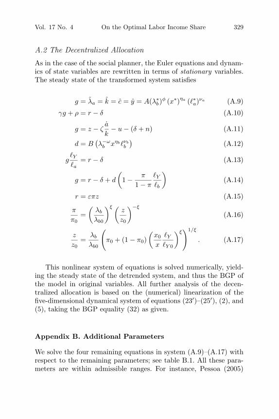
Vol. 17 No. 4 On the Optimal Labor Income Share 329
A.2 The Decentralized Allocation
As in the case of the social planner, the Euler equations and dynam-ics of state variables are rewritten in terms of stationary variables.The steady state of the transformed system satisfies
g = λa = k = c = y = A(λ∗b)
φ (x∗)ηa (∗a)νa (A.9)
γg + ρ = r − δ (A.10)
g = z − ζa
k− u − (δ + n) (A.11)
d = B(λ−ω
b xηbνb
b
)(A.12)
gY
a= r − δ (A.13)
g = r − δ + d
(1 − π
1 − π
Y
b
)(A.14)
r = επz (A.15)
π
π0=
(λb
λb0
)ξ (z
z0
)−ξ
(A.16)
z
z0=
λb
λb0
(π0 + (1 − π0)
(x0
x
Y
Y 0
)ξ)1/ξ
. (A.17)
This nonlinear system of equations is solved numerically, yield-ing the steady state of the detrended system, and thus the BGP ofthe model in original variables. All further analysis of the decen-tralized allocation is based on the (numerical) linearization of thefive-dimensional dynamical system of equations (23′)–(25′), (2), and(5), taking the BGP equality (32) as given.
Appendix B. Additional Parameters
We solve the four remaining equations in system (A.9)–(A.17) withrespect to the remaining parameters; see table B.1. All these para-meters are within admissible ranges. For instance, Pessoa (2005)

330 International Journal of Central Banking October 2021
Table B.1. Baseline Calibration: Additional Parameters
Parameter Value
Labor-Augmenting R&D
Unit Productivity A 0.02Capital Spillover Exponent ηa 0.24
Capital-Augmenting R&D
Unit Productivity B 0.16Capital Spillover Exponent ηb 0.13Degree of Decreasing Returns ω 0.50Obsolescence Rate d 0.08Spillover from Capital- to Labor-Augmenting
Tech. Change φ 0.30
Technology Choice Externality ζ 115.28
estimates values for the obsolescence parameter d between 0 and15 percent; our endogenously determined value is thus centered inthat range. Comparing ηa = 0.24 with ηb = 0.13 signifies that,first of all, positive spillovers of capital intensity in R&D (effec-tive capital augmentation of the R&D process) assuredly matter forR&D productivity, and second, that they are relatively more impor-tant for inventing new labor-augmenting technologies than capital-augmenting ones. Moreover, with φ = 0.3, labor-augmenting R&D—the ultimate engine of long-run growth—is substantially reinforcedby spillovers coming from the capital-augmenting R&D sector. Onthe other hand, ω = 0.5 means that the scope for capital-augmentingR&D is quite strongly limited by decreasing returns. Given thisbenchmark calibration, as we said in the main text, the steady stateis a saddle point.
Appendix C. Robustness Exercises: Impact of ParameterVariation on the Equilibrium Growth Rate
So far we have confirmed the received wisdom that the growth ratein the DA, gDA, is socially suboptimal. This appears to be generallytrue in our model, regardless of its parameterization.

Vol. 17 No. 4 On the Optimal Labor Income Share 331
Figure C.1. Dependence of Equilibrium Growth on ModelParameters
Notes: The real economic growth rate g on vertical axis; corresponding para-meter support on the horizontal axis. Social planner allocation (dashed lines),decentralized equilibrium (solid lines). The vertical dotted line in each graphrepresents the baseline calibrated parameter value.

332 International Journal of Central Banking October 2021
Focusing on a reasonable parameter support, and assuming grosscomplements (see figure C.1), we can however identify a few credi-ble cases where the difference between the two growth rates becomessmall:
• A higher ρ (i.e., more impatience for current consumption),implies less capital and R&D accumulation and lower equi-librium growth than otherwise. If ρ is sufficiently large, thengSP →+ gDA.31
• If the consumption smoothing motive is sufficiently weak (γhigh), then gSP →+ gDA.
• If the capital spillover exponents are weak, νa → 0 or νb → 0,then they attenuate the engine of long-run growth in the R&Dequations and thus pull both gSP and gDA down.
Finally, note, departing from gross substitutes, we see the dra-matic result that as σ (or equivalently ξ) increases, the gap gSP −gDA
hyperbolically widens; conversely, it narrows as substitution possi-bilities tend to zero (the Leontief case). We explore this in the nextappendix.
31See also figure D.1.
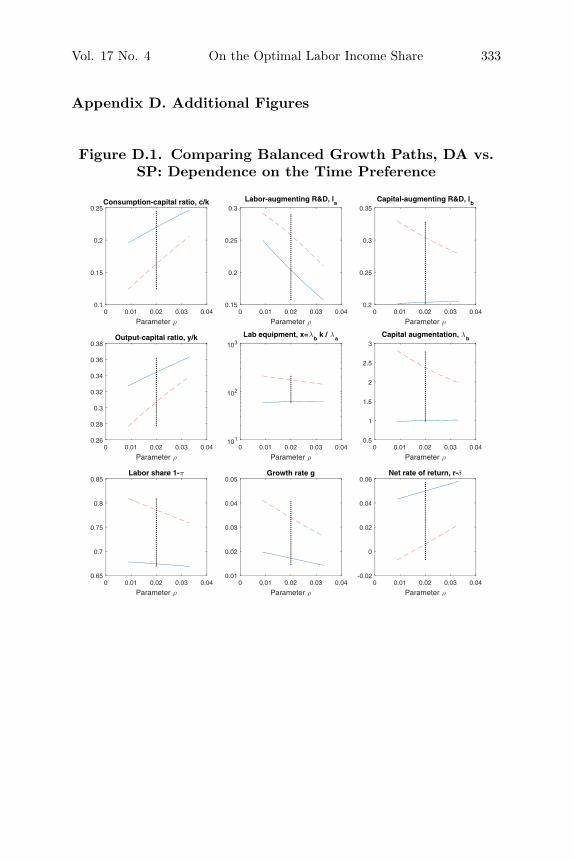
Vol. 17 No. 4 On the Optimal Labor Income Share 333
Appendix D. Additional Figures
Figure D.1. Comparing Balanced Growth Paths, DA vs.SP: Dependence on the Time Preference

334 International Journal of Central Banking October 2021
Figure D.2. Comparing Balanced Growth Paths, DA vs.SP: Dependence on the Intertemporal Elasticity of
Substitution in Consumption

Vol. 17 No. 4 On the Optimal Labor Income Share 335
Figure D.3. Comparing Balanced Growth Paths, DA vs.SP: Dependence on the Capital Spillover Exponent in
Capital-Augmenting R&D

336 International Journal of Central Banking October 2021
Figure D.4. Dependence of Equilibrium Labor Share onModel Parameters, for the Alternative Calibration of
σ = 1.25 (ξ = 0.2)
Notes: 1 − π on vertical axis; corresponding parameter support on the horizon-tal axis. Social planner allocation (dashed lines), decentralized equilibrium (solidlines). The vertical dotted line in each graph represents the baseline calibratedparameter value.

Vol. 17 No. 4 On the Optimal Labor Income Share 337
Figure D.5. Dependence of BGP on Elasticity ofSubstitution, DA vs. SP
Notes: Social planner allocation (dashed lines), decentralized equilibrium (solidlines). The vertical dotted line in each graph represents the baseline calibratedparameter value.
References
Acemoglu, D. 2003. “Labor- and Capital-Augmenting TechnicalChange.” Journal of the European Economic Association 1 (1):1–37.
Alvarez-Pelaez, M. J., and C. Groth 2005. “Too Little or Too MuchR&D?” European Economic Review 49 (2): 437–56.

338 International Journal of Central Banking October 2021
Antras, P. 2004. “Is the U.S. Aggregate Production Function Cobb-Douglas? New Estimates of the Elasticity of Substitution.” Con-tributions to Macroeconomics 4: 1–34.
Arrow, K., H. B. Chenery, B. S. Minhas, and R. M. Solow. 1961.“Capital-Labor Substitution and Economic Efficiency.” Reviewof Economics and Statistics 43: 225–50.
Atkinson, A. B. 2015. Inequality: What Can Be Done? HarvardUniversity Press.
Atkinson, A. B., T. Piketty, and E. Saez. 2011. “Top Incomes in theLong Run of History.” Journal of Economic Literature 49 (1):3–71.
Azariadis, C. 1996. “The Economics of Poverty Traps — Part One:Complete Markets.” Journal of Economic Growth 1 (4): 449–86.
Barro, R. J., and X. X. Sala-i-Martin. 2003. Economic Growth. MITPress.
Benassy, J.-P. 1998. “Is There Always Too Little Research inEndogenous Growth with Expanding Product Variety?” Euro-pean Economic Review 42 (1): 61–69.
Bengtsson, E. 2014. “Labour’s Share in Twentieth-Century Sweden:A Reinterpretation.” Scandinavian Economic History Review62 (3): 290–314.
Caselli, F. 2005. “Accounting for Cross-Country Income Differ-ences.” In Handbook of Economic Growth, Vol. 1A, ed. P. Aghionand S. N. Durlauf, 679–741 (chapter 9). North-Holland.
Charpe, M., S. Bridji, and P. McAdam. 2020. “Labor Share andGrowth in the Long Run.” Macroeconomic Dynamics 24 (7):1720–57.
de La Grandville, O. 1989. “In Quest of the Slutsky Diamond.”American Economic Review 79 (3): 468–81.
———. 2012. “How Much Should a Nation Save? A New Answer.”Studies in Nonlinear Dynamics and Econometrics 16 (2): 1–36.
———. 2016. Economic Growth: A Unified Approach. Second edi-tion. Cambridge University Press.
de Loecker, J., J. Eeckhout, and G. Unger. 2020. “The Rise of MarketPower and the Macroeconomic Implications.” Quarterly Journalof Economics 135 (2): 561–644.
Dixit, A. K., and J. E. Stiglitz. 1977. “Monopolistic Competitionand Optimum Product Diversity.” American Economic Review67 (3): 297–308.

Vol. 17 No. 4 On the Optimal Labor Income Share 339
Galı, J., and M. Gertler. 1999. “Inflation Dynamics: A StructuralEconometric Analysis.” Journal of Monetary Economics 44 (2):195–222.
Groth, C., and J. B. Madsen. 2016. “Medium-term Fluctuations andthe ‘Great Ratios’ of Economic Growth.” Journal of Macroeco-nomics 49 (September): 149–76.
Growiec, J. 2007. “Beyond the Linearity Critique: The Knife-EdgeAssumption of Steady-State Growth.” Economic Theory 31:489–99.
Growiec, J., P. McAdam, and J. Muck. 2018. “Endogenous LaborShare Cycles: Theory and Evidence.” Journal of EconomicDynamics and Control 87 (February): 74–93.
Growiec, J., and J. Muck. 2020. “Isoelastic Elasticity of Substitu-tion Production Functions.” Macroeconomic Dynamics 24 (7):1597–1634.
Guo, J. T., and K. J. Lansing. 2009. “Capital–Labor Substitutionand Equilibrium Indeterminacy.” Journal of Economic Dynamicsand Control 33 (12): 1991–2000.
Herrendorf, B., C. Herrington, and A. Valentinyi. 2015. “SectoralTechnology and Structural Transformation.” American Eco-nomic Journal: Macroeconomics 7 (4): 104–33.
Irmen, A., and A. Tabakovic. 2020. “Factor Income Distributionand Endogenous Economic Growth: Piketty Meets Romer.” Eco-nomic Inquiry 58 (3): 1342–61.
Jaimovich, N., and H. E. Siu. 2020. “Job Polarization and JoblessRecoveries.” Review of Economics and Statistics 102 (1): 129–47.
Jalava, J., M. Pohjola, A. Ripatti, and J. Vilmunen. 2006. “BiasedTechnical Change and Capital–Labor Substitution in Finland,1902-2003.” B.E. Journal of Macroeconomics 6 (1): 1–20.
Jones, C. I. 1995. “R&D-Based Models of Economic Growth.” Jour-nal of Political Economy 103 (4): 759–84.
———. 1999. “Growth: With or Without Scale Effects?” AmericanEconomic Review 89 (2): 139–44.
———. 2005. “Growth and Ideas.” In Handbook of EconomicGrowth, Vol. 1B, ed. P. Aghion and S. N. Durlauf, 1063–1111(chapter 16). North-Holland.
Jones, C. I., and J. C. Williams. 2000. “Too Much of a Good Thing?The Economics of Investment in R&D.” Journal of EconomicGrowth 5 (1): 65–85.

340 International Journal of Central Banking October 2021
Jones, L. E., and R. E. Manuelli. 1990. “A Convex Model of Equi-librium Growth: Theory and Policy Implications.” Journal ofPolitical Economy 98 (5, Part 1): 1008–38.
Kaas, L., and L. von Thadden. 2003. “Unemployment, Factor Sub-stitution and Capital Formation.” German Economic Review4 (4): 475–95.
Karabarbounis, L., and B. Neiman. 2014. “The Global Decline of theLabor Share.” Quarterly Journal of Economics 129 (1): 61–103.
Kennedy, C. 1964. “Induced Bias in Innovation and the Theory ofDistribution.” Economic Journal 74 (295): 541–47.
Klump, R. 2002. “Verteilung und Wirtschaftswachstum: Eine neok-lassische Verallgemeinerung des Wachstumsmodell von Kaldor.”In Zur Theorie, Empirie und Politik der Einkommensverteilung,ed. L. Menkhoff and F. Sell, 11–26. Berlin-Heidelberg-New York:Springer.
Klump, R., and O. de La Grandville. 2000. “Economic Growth andthe Elasticity of Substitution: Two Theorems and Some Sugges-tions.” American Economic Review 90 (1): 282–91.
Klump, R., P. McAdam, and A. Willman. 2007. “Factor Substitutionand Factor-Augmenting Technical Progress in the US.” Reviewof Economics and Statistics 89 (1): 183–92.
———. 2012. “The Normalized CES Production Functions: Theoryand Empirics.” Journal of Economic Surveys 26 (5): 769–99.
Klump, R., and H. Preissler. 2000. “CES Production Functions andEconomic Growth.” Scandinavian Journal of Economics 102 (1):41–56.
Knoblach, M., and F. Stockl. 2020. “What Determines the Elas-ticity of Substitution between Capital and Labor? A LiteratureReview.” Journal of Economic Surveys 34 (4): 847–75.
Kortum, S. 1993. “Equilibrium R&D and the Patent-R&D Ratio:U.S. Evidence.” American Economic Review 83 (2): 450–57.
Laeven, L., P. McAdam, and A. Popov. 2018. “Credit Shocks,Employment Protection, and Growth: Firm-level Evidence fromSpain.” ECB Working Paper No. 2166.
Leon-Ledesma, M. A., P. McAdam, and A. Willman. 2010. “Identify-ing the Elasticity of Substitution with Biased Technical Change.”American Economic Review 100 (4): 1330–57.
Leon-Ledesma, M. A., and M. Satchi. 2019. “Appropriate Technol-ogy and Balanced Growth.” Review of Economic Studies 86 (2):807–35.
Vol. 17 No. 4 On the Optimal Labor Income Share 341
Li, C.-W. 2000. “Endogenous vs. Semi-endogenous Growth in a Two-R&D-Sector Model.” Economic Journal 110 (462): C109–C122.
Liesner, T. 1989. One Hundred Years of Economic Statistics. Factson File Publications.
McAdam, P., and A. Willman. 2004. “Supply, Factor Shares andInflation Persistence: Re-Examining Euro-Area New-KeynesianPhillips Curves.” Oxford Bulletin of Economics and Statistics66 (s1): 637–70.
———. 2013. “Medium Run Redux.” Macroeconomic Dynamics17 (4): 695–727.
Muck, J. 2017. “Elasticity of Substitution between Labor andCapital: Robust Evidence from Developed Economies.” Work-ing Paper No. 271, Narodowy Bank Polski, Economic ResearchDepartment.
Muck, J., P. McAdam, and J. Growiec. 2018. “Will the ‘True’ LaborShare Stand Up? An Applied Survey on Labor Share Measures.”Journal of Economic Surveys 32 (4): 961–84.
Oberfield, E., and D. Raval. 2018. “Micro Data and Macro Technol-ogy.” Econometrica 89 (2): 703–32.
Palivos, T., and G. Karagiannis. 2010. “The Elasticity of Substitu-tion as an Engine of Growth.” Macroeconomic Dynamics 14 (5):617–28.
Pessoa, A. 2005. “‘Ideas’ Driven Growth: The OECD Evidence.”Portuguese Economic Journal 4 (1): 46–67.
Piketty, T. 2014. Capital in the Twenty-First Century. Harvard Uni-versity Press. Translated from French by Arthur Goldhammer.
Piketty, T., and G. Zucman. 2014. “Capital is Back: Wealth–IncomeRatios in Rich Countries, 1700–2010.” Quarterly Journal of Eco-nomics 129 (3): 1255–1310.
Pitchford, J. 1960. “Growth and the Elasticity of Factor Substitu-tion.” Economic Record 36 (76): 491–504.
Ramsey, F. P. 1928. “A Mathematical Theory of Saving.” EconomicJournal 38 (152): 543–59.
Romer, P. M. 1990. “Endogenous Technological Change.” Journalof Political Economy 98 (5, Part 2): S71–S102.
Rowthorn, R. 1999. “Unemployment, Wage Bargaining and Capital–Labour Substitution.” Cambridge Journal of Economics 23 (4):413–25.

342 International Journal of Central Banking October 2021
Saam, M. 2008. “Openness to Trade as a Determinant of the Macro-economic Elasticity of Substitution.” Journal of Macroeconomics30 (2): 691–702.
Solow, R. M. 1960. “Investment and Technical Progress.” In Mathe-matical Methods in the Social Sciences, ed. K. Arrow, S. Karlin,and P. Suppes, 89–104. Stanford University Press.
Uzawa, H. 1961. “Neutral Inventions and the Stability of GrowthEquilibrium.” Review of Economic Studies 28 (1): 117–24.