arX

iv:1

110.

6078

v1 [

mat

h.O

C]

27

Oct

201

1 On the Mathematical Structure of

Balanced Chemical Reaction Networks

Governed by Mass Action Kinetics

Arjan van der Schaft∗ Shodhan Rao† Bayu Jayawardhana‡

October 28, 2011

Abstract

Motivated by recent progress on the interplay between graph the-ory, dynamics, and systems theory, we revisit the analysis of chemicalreaction networks described by mass action kinetics. For reaction net-works possessing a thermodynamic equilibrium we derive a compactformulation exhibiting at the same time the structure of the complexgraph and the stoichiometry of the network, and which admits a di-rect thermodynamical interpretation. This formulation allows us toeasily characterize the set of equilibria and their stability properties.Furthermore, we develop a framework for interconnection of chemicalreaction networks. Finally we discuss how the established frameworkleads to a new approach for model reduction.

1 Introduction

Large-scale chemical reaction networks arise abundantly in bio-engineeringand systems biology. A very simple example involving only two chemicalreactions in the glycolytic pathway is given by the following two coupledreactions

Acetoacetyl ACP + NADPH +H+⇋ D-3-Hydroxybutyryl ACP + NADP+

D-3-Hydroxybutyryl ACP ⇋ crotonyl ACP + H2O. (1)

∗Johann Bernoulli Institute for Mathematics and Computer Science, University ofGroningen, e-mail: A.J.van.der.Schaft@rug.nl

†Systems Biology Centre for Energy Metabolism and Ageing, University of Groningen,email: s.rao@umcg.nl

‡Discrete Technology and Production Automation, University of Groningen, email:b.jayawardhana@rug.nl

The compounds Acetoacetyl ACP, NADPH, H+, D-3-Hydroxybutyryl ACP,NADP, crotonyl ACP and H2O involved in the reaction network are calledthe chemical species of the network. The most basic law prescribing thedynamics of the concentrations of the various species involved in a chemicalreaction network is the law of mass action kinetics, leading to polynomialdifferential equations for the dynamics of each species. Large-scale networksthus lead to a high-dimensional set of coupled polynomial differential equa-tions, which are usually difficult to analyze.

In order to gain insight into the dynamical properties of complex re-action networks it is important to identify their underlying mathematicalstructure, and to express their dynamics in the most compact way. In linewith the recent surge of interest in network dynamics at least two aspectsshould be fundamental in such a mathematical formulation: (1) a graphrepresentation, and (2) a specific form of the differential equations.

The graph representation of chemical reaction networks is not immediate,since a chemical reaction (the obvious candidate for identification with theedges of a graph) generally involves more than two chemical species (themost basic candidate for identification with the vertices). We will followan approach that has been initiated and developed in the work of Horn &Jackson [14, 13] and Feinberg, see e.g. [10, 11], by associating the complexesof the chemical reaction network (i.e., the left- and right-hand sides of thereactions) with the vertices of the graph1. The resulting directed graph,called the complex graph in this paper, is characterized by its incidencematrix. The expression of the complexes in the chemical species defines anextended stoichiometric matrix, called the complex stoichiometric matrix,which is immediately related to the standard stoichiometric matrix throughthe incidence matrix of the complex graph; see e.g. [21], [2].

In order to derive a specific form of differential equations we will startwith the basic assumption that the chemical reaction rates are governed bymass action kinetics. As an initial step we then derive a compact form ofthe dynamics involving a non-symmetric weighted Laplacian matrix of thecomplex graph. The basic form of these equations can be already foundin the innovative paper by Sontag [23]. The main part of the paper ishowever devoted to a subclass of mass action kinetics chemical reaction net-works, where we assume the existence of a thermodynamical equilibrium,or equivalently, where the detailed balance equations are assumed to admita solution. We will call such chemical reaction networks balanced chemi-

1For alternative approaches based on species-reaction graphs and Petri-nets we referto e.g. [6, 7, 2].

cal reaction networks. Balanced chemical reaction networks are necessarilyreversible but involve additional conditions on the forward and reverse re-action rate constants (usually referred to as the Wegscheider conditions; see[12]). For such balanced chemical reaction networks we will be able to derivea particularly elegant form of the dynamics, involving a symmetric weightedLaplacian matrix of the complex graph. Furthermore, it turns out that thisform has a direct thermodynamical interpretation, and in fact can be re-garded as a graph-theoretic version of the formulation derived in the workof Katchalsky, Oster & Perelson [19, 18].

The obtained form of the equations of balanced chemical reaction net-works will be used to give, in a very simple and insightful way, a characteri-zation of the set of equilibria, and a proof of the asymptotic convergence toa unique thermodynamic equilibrium corresponding to the initial conditionof the system. Similar results for a different class of mass action kinet-ics reaction networks, in particular weakly reversible networks with zero-deficiency, have been derived in the fundamental work of Horn [13] andFeinberg [10, 11], which was an indispensable source of concepts and toolsfor the work reported in this paper.

Subsequently we show how this form of the dynamics of chemical re-action networks can be extended to open reaction networks; i.e., networksinvolving an influx or efflux of some of the chemical species, called the bound-ary chemical species. Furthermore, we show how corresponding outputs canbe defined as the chemical potentials of these boundary chemical speciesand how this leads to a physical theory of interconnection of open reactionnetworks, continuing upon the work of Oster & Perelson [18, 20].

In the final part of the paper we make some initial steps in showinghow the derived form of balanced reaction networks can be utilized to de-rive in a systematic way reduced-order models. This reduction procedure isbased on the Laplacian matrix of the complex graph, and draws inspirationfrom a similar technique in electrical circuit theory, sometimes referred to asKron reduction. The model reduction procedure leads to an approximatingreduced-order model which is again a mass action kinetics balanced chemicalreaction network.

Interestingly enough, the derived form of the equations of chemical reac-tion networks involving a weighted Laplacian matrix of the complex graphis reminiscent of the dynamics of the standard consensus algorithm of multi-agent systems, see e.g. [17]. In fact, the form of the stability analysis in bothcases is quite similar. Furthermore, the relation between the initial concen-tration of chemical species and the unique final equilibrium concentration isclosely related to the recent concept of χ-consensus in [5].

The paper is organized as follows. In Section 2, we summarize themathematical structure of a network of chemical reactions described in e.g.[14, 13, 10, 11, 21]; see also [2] for a clear account. In Section 3, we recall thelaw of mass action kinetics, and derive a general graph-theoretic formula-tion which is basically already contained in the innovative paper by Sontag[23]. Next, for the important subclass of chemical reaction networks admit-ting a thermodynamic equilibrium (balanced reaction networks) we derive aparticularly simple formulation involving a symmetric weighted Laplacianmatrix for the complex graph. Before providing the thermodynamical in-terpretation of this formulation, we discuss the graph-theoretic treatmentof the complex graph, largely following the exposition in [21], and its im-plications for the established formulation of balanced reaction networks. InSection 4 we utilize the developed formulation to derive a simple character-ization of the set of equilibria, and we give a Lyapunov analysis to show theconvergence to a unique equilibrium depending on the initial concentrationvector. At the end of this section we comment on the relation with consen-sus algorithms. In Section 5 the framework is extended to reaction networkswith inflows and outflows, and we discuss interconnection of such reactionnetworks through shared boundary chemical species. The initial steps in theapplication of the established formulation of balanced reaction networks tomodel reduction are discussed in Section 6. Finally, Section 7 contains theconclusions, and some topics of ongoing research.

Notation: The space of n dimensional real vectors is denoted by Rn, and

the space of m× n real matrices by Rm×n. The space of n dimensional real

vectors consisting of all strictly positive entries is denoted by Rn+ and the

space of n dimensional real vectors consisting of all nonnegative entries isdenoted by R

n+. The rank of a real matrix A is denoted by rankA. Given

a1, . . . , an ∈ R, diag(a1, . . . , an) denotes the diagonal matrix with diagonalentries a1, . . . , an; this notation is extended to the block-diagonal case whena1, . . . , an are real square matrices. Furthermore, kerA and spanA denotethe kernel and span respectively of a real matrix A. If U denotes a linearsubspace of Rm, then U⊥ denotes its orthogonal subspace (with respect tothe standard Euclidian inner product). 1m denotes a vector of dimension mwith all entries equal to 1. The time-derivative dx

dt(t) of a vector x depending

on time t will be usually denoted by x.Define the mapping Ln : Rm

+ → Rm, x 7→ Ln(x), as the mapping whose

i-th component is given as (Ln(x))i := ln(xi). Similarly, define the mappingExp : Rm → R

m+ , x 7→ Exp(x), as the mapping whose i-th component

is given as (Exp(x))i := exp(xi). Also, define for any vectors x, z ∈ Rm

the vector x · z ∈ Rm as the element-wise product (x · z)i := xizi, i =

1, 2, . . . ,m, and the vector xz∈ R

m as the element-wise quotient(

xz

)

i:=

xi

zi, i = 1, · · · ,m. Note that with these notations Exp(x + z) = Exp(x) ·

Exp(z) and Ln(x · z) = Ln(x) + Ln(z),Ln(

xz

)

= Ln(x)− Ln(z).

2 Chemical reaction network structure

In this section we will survey the basic topological structure of chemical re-action networks. First step is the stoichiometry expressing the conservationlaws of chemical reactions. A next innovative step was taken in the work ofHorn & Jackson and Feinberg [14, 13, 10, 11] by defining the complexes ofa reaction to be the vertices of a graph. We will summarize these achieve-ments in a slightly more abstract manner, also making use of the expositiongiven in [21]; see also [2] for a nice account.

2.1 Stoichiometry

Consider a chemical reaction network involving m chemical species (metabo-lites), among which r chemical reactions take place. The basic structureunderlying the dynamics of the vector x ∈ R

m+ of concentrations xi, i =

1, · · · ,m, of the chemical species is given by the balance laws

x = Sv, (2)

where S is an m× r matrix, called the stoichiometric matrix. The elementsof the vector v ∈ R

r are commonly called the (reaction) fluxes. The stoichio-metric matrix S, which consists of (positive and negative) integer elements,captures the basic conservation laws of the reactions. For example, thestoichiometric matrix of the two coupled reactions involving the chemicalspecies X1,X2,X3 given as

X1 + 2X2 ⇋ X3 ⇋ 2X1 +X2

is

S =

−1 2−2 11 −1

,

while the first reversible reaction in (1)

Acetoacetyl ACP+NADPH+H+⇋ D-3-Hydroxybutyryl ACP+NADP+

involving the species {Acetoacetyl ACP, NADPH, H+, D-3-HydroxybutyrylACP, NADP+, crotonyl ACP, H2O} has the stoichiometric matrix

S =[

−1 −1 −1 1 1 0]T

In many cases of interest, especially in biochemical reaction networks, chem-ical reaction networks are intrinsically open, in the sense that there is acontinuous exchange with the environment (in particular, flow of chemicalspecies and connection to other reaction networks). This will be modeled bya vector vb ∈ R

b consisting of b boundary fluxes vb, leading to an extendedmodel

x = Sv + Sbvb (3)

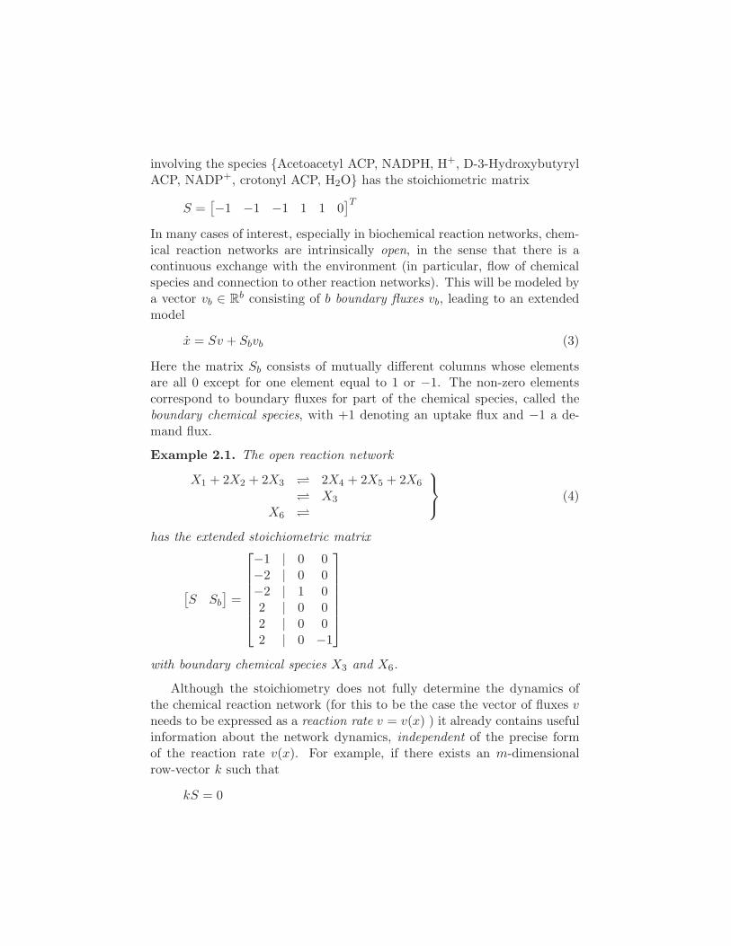
Here the matrix Sb consists of mutually different columns whose elementsare all 0 except for one element equal to 1 or −1. The non-zero elementscorrespond to boundary fluxes for part of the chemical species, called theboundary chemical species, with +1 denoting an uptake flux and −1 a de-mand flux.

Example 2.1. The open reaction network

X1 + 2X2 + 2X3 ⇋ 2X4 + 2X5 + 2X6

⇋ X3

X6 ⇋

(4)

has the extended stoichiometric matrix

[

S Sb

]

=

−1 | 0 0−2 | 0 0−2 | 1 02 | 0 02 | 0 02 | 0 −1

with boundary chemical species X3 and X6.

Although the stoichiometry does not fully determine the dynamics ofthe chemical reaction network (for this to be the case the vector of fluxes vneeds to be expressed as a reaction rate v = v(x) ) it already contains usefulinformation about the network dynamics, independent of the precise formof the reaction rate v(x). For example, if there exists an m-dimensionalrow-vector k such that

kS = 0

then the quantity kx is a conserved quantity for the dynamics x = Sv(x) forall possible reaction rates v = v(x). Indeed, d

dtkx = kSv(x) = 0. If k ∈ R

m+ ,

then the quantity kx is commonly called a conserved moiety. Geometrically,for all possible fluxes the solutions of the differential equations x = Sv(x)starting from an initial state x0 will always remain within the affine spacex0 + imS. In case of an open chemical reaction network d

dtkx = 0 modifies

into

d

dtkx = kSbvb,

expressing that the time-evolution of the quantity kx only depends on theboundary fluxes vb.

2.2 The complex graph

The network structure of a chemical reaction network cannot be directlycaptured by a graph involving the chemical species (since generally thereare more than two species involved in a reaction). Instead, we will follow anapproach originating in the work of Horn & Jackson [14, 13] and Feinberg[10, 11], introducing the space of complexes. The set of complexes of achemical reaction network is simply defined as the union of all the differentleft- and right-hand sides (substrates and products) of the reactions in thenetwork.

For example, the reaction network in (1) entails four complexes, namelythe substrates Acetoacetyl ACP+ NADPH +H+ and D-3-HydroxybutyrylACP+NADP+, and the products D-3-Hydroxybutyryl ACP and crotonylACP +H2O. In general, a product complex of one reaction may be thesubstrate complex of another. Thus, the complexes corresponding to thetwo reactions

2X1 ⇋ X1 + 2X2 ⇋ X2 +X3

are 2X1,X1+X2 andX2+X3. A complex may also be the product/substratecomplex of more than one reaction.

The expression of the complexes in terms of the chemical species is for-malized by an m× c matrix Z, whose ρ-th column captures the expressionof the ρ-th complex in the m chemical species. For example, the columnexpressing the complex X1 + 2X2 + 2X3 in the chemical reactions (4) is

[

1 2 2 0 0 0]T

Note that by definition all elements of the matrix Z are non-negative inte-gers.

Since the complexes are left- and right-hand sides of the reactions theycan be naturally associated with the vertices of a directed graph, with edgescorresponding to the reactions. The complexes on the left-hand side ofthe reactions are called the substrate complexes and those on the right-handside of the reactions are called the product complexes. Formally, the reactionσ ⇋ π between the σ-th and the π-th complex defines a directed edge withtail vertex being the σ-th complex and head vertex being the π-th complex.The resulting graph is called the complex graph.

Recall, see e.g. [3], that any directed graph is defined by its incidencematrix B. This is an c × r matrix, c being the number of vertices and rbeing the number of edges, with (ρ, j)-th element equal to −1 if vertex ρ isthe tail vertex of edge j and 1 if vertex ρ is the head vertex of edge j, while0 otherwise. Obviously there is a close relation between the matrix Z andthe stoichiometric matrix S, which is expressed as

S = ZB, (5)

with B the incidence matrix of the complex graph. For this reason we willcall Z the complex stoichiometric matrix. Hence the relation x = Sv betweenthe fluxes v through the chemical reaction network and the time-derivativeof vector of chemical species x, cf. (2), can be also written as

x = ZBv, (6)

with the vector Bv belonging to the space of complexes Rc.

3 The dynamics of mass action kinetics chemical

reaction networks

In this section we will derive a compact form for the dynamics of a chemicalreaction network, whose reactions are described by mass action kinetics.After deriving a general form in Section 3.1 we will focus in the rest of thesection on balanced chemical reaction networks. The resulting form of thedynamical equations for balanced reaction networks will be fundamental tothe analysis of this dynamics in the subsequent sections.

3.1 The general form of mass action kinetics

The dynamics of the concentration vector x (or equivalently, in case of afixed volume, the vector n of mole numbers) is given once the internal fluxes

v are specified as a function v = v(x) of x, defining the reaction rates. Themost basic model for specifying the reaction rates is mass action kinetics,defined as follows. Consider the single reaction

X1 +X2 ⇋ X3,

involving the three chemical speciesX1,X2,X3 with concentrations x1, x2, x3.In mass action kinetics the reaction is considered to be a combination of theforward reaction X1 +X2 ⇀ X3 with forward rate equation vforw(x1, x2) =kforwx1x2 and the reverse reaction X1 + X2 ↽ X3, with rate equationvrev(x3) = krevx3. The constants kforw, krev are called respectively theforward and reverse reaction constants. The net reaction rate given by massaction kinetics is thus

v(x1, x2, x3) = vforw(x1, x2)− vrev(x3) = kforwx1x2 − krevx3

In general, the mass action reaction rate of the j-th reaction of a chemicalreaction network, from a substrate complex Sj to a product complex Pj , isgiven as

vj(x) = kforwj

m∏

i=1

xZiSj

i − krevj

m∏

i=1

xZiPj

i , (7)

where Ziρ is the (i, ρ)-th element of the complex stoichiometric matrix Z,and kforwj , krevj ≥ 0 are the forward/reverse reaction constants of the j-threaction, respectively. Without loss of generality we will throughout assumethat for every j the constants kforwj , krevj are not both equal to zero (since inthis case the j-th reaction is not active).

This can be rewritten in the following way. Let ZSjand ZPj

denotethe columns of the complex stoichiometry matrix Z corresponding to thesubstrate and the product complexes of the j-th reaction. Using the mappingLn : Rc

+ → Rc as defined at the end of the Introduction, the mass action

reaction equation (7) for the j-th reaction from substrate complex Sj toproduct complex Pj can be rewritten as

vj(x) = kforwj exp(

ZTSjLn(x)

)

− krevj exp(

ZTPjLn(x)

)

. (8)

Based on the formulation in (8), we can describe the complete reactionnetwork dynamics as follows. Let the mass action rate for the complete set

of reactions be given by the vector v(x) =[

v1(x) · · · vr(x)]T

. For everyσ, π ∈ {1, · · · , c}, denote by aσπ = krevj , aπσ = kforwj if (σ, π) = (Sj ,Pj),

j ∈ {1, . . . , r} and aσπ = 0 elsewhere. Define the weighted adjacency matrixA of the complex graph2 as the matrix with (σ, π)-th element aσπ, whereσ, π ∈ {1, · · · , c}. Furthermore, define the weighted Laplacian matrix L asthe c× c matrix

L := ∆−A (9)

where ∆ is the diagonal matrix whose (ρ, ρ)-th element is equal to the sumof the elements of the ρ-th column of A. Then it can be verified that thevector Bv(x) for the mass action reaction rate vector v(x) is equal to

Bv(x) = −LExp(

ZTLn(x))

,

where the mapping Exp : Rc → R

c+ has been defined at the end of the

Introduction. Hence the dynamics can be compactly written as

x = −ZLExp(

ZTLn(x))

(10)

A similar expression of the dynamics corresponding to mass action kinetics,in less explicit form, was already obtained in [23].

3.2 Balanced mass action kinetics

In the rest of this paper we will focus on an important subclass of massaction chemical reaction networks. We need the following basic notions.

Definition 3.1. A vector of concentrations x∗ ∈ Rm+ is called an equilib-

rium3 for the dynamics x = Sv(x) if

Sv(x∗) = 0

Furthermore, x∗ ∈ Rm+ is called a thermodynamic equilibrium if

v(x∗) = 0

Clearly, any thermodynamic equilibrium is an equilibrium, but not nec-essarily the other way around (since in general S = ZB is not injective).

2Strictly speaking, A is the adjacency matrix not of the complex graph, but of a directedaugmented graph. Each j-th edge of the complex graph is replaced by two directed edges:one corresponding to the forward reaction with weight kforw

j and one corresponding to thereverse reaction with weight krev

j .3Sometimes called a kinetic equilibrium, in order to distinguish it from a thermody-

namical equilibrium.

3.2.1 The existence of thermodynamic equilibria

Necessary and sufficient conditions for the existence of a thermodynamicequilibrium can be derived in the following linear-algebraic way following[12]. These conditions are usually referred to as the Wegscheider conditions,generalizing the classical results of [24].

Consider the j-th reaction from substrate Sj to product Pj , describedby the mass action rate equation

(

see (8))

vj(x) = kforwj exp(

ZTSjLn(x)

)

− krevj exp(

ZTPjLn(x)

)

Then x∗ ∈ Rm+ is a thermodynamic equilibrium, i.e., v(x∗) = 0, if and only

if

kforwj exp(

ZTSjLn(x∗)

)

= krevj exp(

ZTPjLn(x∗)

)

, j = 1, · · · , r (11)

The equations (11), sometimes referred to as the detailed balance equations,can be rewritten as follows. Define the equilibrium constant Keq

j of the j-threaction as (assuming krevj 6= 0)

Keqj :=

kforwj

krevj

(12)

Then the detailed balance equations (11) are seen to be equivalent to

Keqj = exp

(

ZTPjLn(x∗)− ZT

SjLn(x∗)

)

, j = 1, · · · , r (13)

Collecting all reactions, and making use of the incidence matrix B of thecomplex graph, this amounts to the vector equation

Keq = Exp(

BTZTLn(x∗))

= Exp(

STLn(x∗))

, (14)

where Keq is the r-dimensional vector with j-th element Keqj , j = 1, · · · , r.

From here it is easy to characterize the existence of a thermodynamicequilibrium.

Proposition 3.2. There exists a thermodynamic equilibrium x∗ ∈ Rm+ if

and only if kforwj > 0, krevj > 0, for all j = 1, · · · , r, and furthermore

Ln (Keq) ∈ imST (15)

Proof. Clearly kforwj > 0, krevj > 0, j = 1, · · · , r, is a necessary condition forthe existence of a thermodynamic equilibrium. The existence of a vectorLn(x∗), x∗ ∈ R

m+ , satisfying (14) is obviously equivalent to (15). �

It also follows that once a thermodynamic equilibrium x∗ is given, theset of all thermodynamic equilibria is described as follows.

Proposition 3.3. Let x∗ ∈ Rm+ be a thermodynamic equilibrium, then the

set of all thermodynamic equilibria is given by

E := {x∗∗ ∈ Rm+ | S

TLn (x∗∗) = STLn (x∗)} (16)

For ease of exposition we will henceforth refer to mass action chemicalnetworks possessing a thermodynamic equilibrium x∗ ∈ R

m+ as balanced mass

action chemical networks:

Definition 3.4. A chemical reaction network x = Sv(x) governed by massaction kinetics is called balanced if there exists a thermodynamic equilibriumx∗ ∈ R

m+ .

As stated in Proposition 3.2, a necessary condition for the existence ofa thermodynamic equilibrium is the fact that for all reactions the forwardand reverse reaction constants are both strictly positive. Thus all reactionsof a balanced reaction network need to be at least reversible.

Remark 3.5. Usually the conditions (15) are rewritten in the followingmore constructive form. By basic linear algebra (15) is satisfied if and onlyif for all row-vectors σ satisfying σST = 0 we have

r∑

j=1

σj lnKeqj = 0 (17)

Putting back in the definition of the equilibrium constants (12) this is seento be equivalent to the usual form of the Wegscheider conditions4

r∏

j=1

(

kforwj

)σj

=

r∏

j=1

(

krevj

)σj . (18)

4Note that (18) only needs to be checked for a maximally independent set of row-vectors σ satisfying σST = 0. Furthermore, by writing this as σST = σBTZT = 0 thiscan be related to the topological structure of the complex graph and to the deficiency ofthe network; cf. [12]. Furthermore, the Wegscheider conditions admit a thermodynamicalinterpretation, since they are intimately related to the passivity properties of the networkand the independence of the increase of Gibbs’ energy of the path in the reaction network;see also [18, 19].

3.2.2 The standard form of balanced mass action reaction net-

works

For balanced mass action chemical reaction networks we can further rewritethe dynamics (10) in the following useful way. Let x∗ ∈ R

m+ be a thermody-

namic equilibrium, i.e., v(x∗) = 0. Consider the rewritten form (13) of the‘detailed balance’ equations. These equations allow us to define the balancedreaction constant5 of the j-th reaction as

κj(x∗) := kforwj exp

(

ZTSjLn(x∗)

)

= krevj exp(

ZTPjLn(x∗)

)

, j = 1, · · · , r

(19)

Then the mass action reaction rate of the j-th reaction can be written as

vj(x) = κj(x∗)[

exp(

ZTSjLn

( x

x∗

))

− exp(

ZTPjLn

( x

x∗

))]

,

where for any vectors x, z ∈ Rm the quotient vector x

z∈ R

m is definedelementwise (see the end of the Introduction). Defining the r × r diagonalmatrix of balanced reaction constants as

K(x∗) := diag(

κ1(x∗), · · · , κr(x

∗))

(20)

it follows that the mass action reaction rate vector of a balanced reactionnetwork can be written as

v(x) = −K(x∗)BTExp(

ZTLn( x

x∗

))

,

and thus the dynamics of a balanced reaction network takes the form

x = −ZBK(x∗)BTExp(

ZTLn( x

x∗

))

, K(x∗) > 0 (21)

This form will be the starting point for the analysis of balanced chemicalreaction networks in the rest of this paper.

The matrix BK(x∗)BT in (21) again defines a weighted Laplacian matrixfor the complex graph, with weights given by the balanced reaction constantsκ1(x

∗), · · · ,κr(x∗). Note that this is in general a different weighted Laplacian

matrix than the one obtained before, cf. (9). In particular, a main differenceis that the weighted Laplacian BK(x∗)BT is necessarily symmetric. Among

5Although these constants appear in the literature, see e.g. [18, 19], we could not finda standard name for them. Note that κj(x

∗) > 0 is defined as the common value of theforward and reverse reaction rate of the j-th reaction at thermodynamic equilibrium.

others, cf. [3], this implies that the Laplacian BK(x∗)BT is in fact inde-pendent of the orientation of the graph. Thus we may replace any reactionS ⇋ P by P ⇋ S without altering the Laplacian BK(x∗)BT , in agreementwith the usual understanding of a reversible reaction network. The sym-metrization of the Laplacian has been accomplished by the modification ofLn(x) into Ln

(

xx∗

)

, and using the assumption that x∗ is a thermodynamicequilibrium.

Note that K(x∗), and therefore the Laplacian matrix BK(x∗)BT , is inprinciple dependent on the choice of the thermodynamic equilibrium x∗. Inthe next Section 3.3 we will see that actually this dependence is minor: for aconnected complex graph the matrix K(x∗) is, up to a positive multiplicativefactor, independent of the choice of the thermodynamic equilibrium x∗.

3.3 The linkage classes of the complex graph

The complex graph provides a number of tools for the analysis of reactionnetworks. Recall that for any directed graph [3]

rankB = rankL = c− ℓ, (22)

where c is the number of vertices of the graph, and ℓ is equal to the numberof components6 of the complex graph , the linkage classes in the terminologyof [14, 10, 11]. Furthermore, if there is one linkage class in the network (i.e.,the graph is connected and rankB = rankL = c− 1), then

kerL = kerBT = span1c,

where as before 1c is the c-dimensional vector with elements all equal to 1.In general, if the reaction network has ℓ linkage classes then the network

can be decomposed as follows. Let the p-th linkage class have rp reactionsbetween cp complexes. Partition Z, B and K matrices according to the

6A directed graph is connected if there is a path (a number of un-oriented edges)between every two distinct vertices of the graph. The components of a directed graph arethe maximal connected subgraphs.

various linkage classes as

Z =[

Z1 Z2 . . . Zℓ

]

B =

B1 0 0 . . . 00 B2 0 . . . 0...

.... . .

......

0 . . . 0 Bℓ−1 00 . . . . . . 0 Bℓ

K(x∗) = diag(

K1(x∗),K2(x

∗), . . . ,Kℓ(x∗))

(23)

where for p = 1, . . . , ℓ, Zp ∈ Rm×cp+ , Bp ∈ R

cp×rp and Kp ∈ Rrp×rp+ denote,

respectively, the complex stoichiometric matrix, incidence matrix and thediagonal matrix of balanced reaction constants for the p-th linkage class.Furthermore, Sp = ZpBp is the stoichiometric matrix of the p-th linkageclass. It follows that equation (21) can be expanded as

x = −

ℓ∑

p=1

ZpBpKp(x∗)BT

p Exp(

ZTp Ln

( x

x∗

))

, (24)

expressing the contributions of each linkage class to the chemical reactions7.

The above expressions also yield the following alternative characteri-zation of the set of thermodynamic equilibria E given in (16). Since for aconnected graph kerBT = span1c, the set E can be equivalently representedas, writing ST = BTZT ,

E = {x∗∗ ∈ Rm+ | Z

TLn (x∗∗)− ZTLn (x∗) ∈ span1c} (25)

For non-connected graphs the same formula holds for every component.This observation has the following useful consequence.

Proposition 3.6. Consider the definition of the diagonal matrix K(x∗) ofbalanced reaction constants in (20), and the formulation of the dynamicsgiven in (21) for a particular thermodynamic equilibrium x∗. Assume that

7Note that this yields a conserved moiety for the reaction network. In fact, the law

of conservation of mass states that for any complex stoichiometric matrix Z there existsu ∈ R

m+ , such that Z⊤

p u ∈ span1cp for p = 1, . . . , ℓ. Since BTp 1cp = 0, this implies that

u⊤x is a conserved moiety for x = ZBv(x), for all forms of the reaction rate v(x).

the complex graph is connected. Then for any other thermodynamic equilib-rium x∗∗ there exists a positive constant d∗∗ such that

K(x∗∗) = d∗∗K(x∗), Exp(ZTLn( x

x∗∗

)

) =1

d∗∗Exp(ZTLn

( x

x∗

)

)

Furthermore, for a non-connected complex graph there exist positive con-stants d∗∗p , p = 1, · · · , ℓ, such that for each p-th linkage class the diagonalmatrix Kp(x

∗) given in (23) satisfies

Kp(x∗∗) = d∗∗p Kp(x

∗), p = 1, · · · , ℓ

Proof. Assume that the complex graph is connected. Then by (25) thereexists a constant c∗∗ such that ZTLn(x∗∗) = ZTLn(x∗) + c∗∗1. Hence bythe definition of the balanced reaction constants κj in (19) we have

κj(x∗∗) = kforwj exp

(

ZTSjLn(x∗∗)

)

= kforwj exp(

ZTSjLn(x∗) + c∗∗

)

= d∗∗kforwj exp(

ZTSjLn(x∗)

)

= d∗∗κj(x∗),

with d∗∗ := exp(c∗∗) > 0, for each j = 1, · · · , r. The rest follows easily. �

Hence the weighted Laplacian matrix BK(x∗)BT is, up to a multiplica-tive factor, independent of the choice of the thermodynamic equilibrium x∗.The properties of this matrix (e.g., its eigenvalue distribution8) thereforemay serve as an important indicator of the network dynamics. In Section 6we will exploit the Laplacian matrix for model reduction purposes.

3.4 Deficiency

An important notion to relate the structure of the complex graph to thestoichiometry, as introduced in the work of Feinberg [10], is the notion ofdeficiency.

Definition 3.7. The deficiency of a chemical reaction network with complexstoichiometric matrix Z and incidence matrix B is defined as

δ := rankB − rankZB = rankB − rankS ≥ 0 (26)

A reaction network is said to have zero-deficiency if δ = 0.

8Note that the set of eigenvalues of BK(x∗)BT consists of 0 (with multiplicity equalto the number of components) and strictly positive real numbers, cf. [3].

Note that zero-deficiency is equivalent to

kerZ ∩ imB = 0,

or to the mapping Z : imB ⊂ Rc → R

m being injective. Hence in thezero-deficiency case there is a one-to-one correspondence between the ratevector x ∈ imS ⊂ R

m of chemical species x ∈ Rm+ and the rate vector

y ∈ imB ⊂ Rc of complexes y ∈ R

c. Many chemical reaction networks arezero-deficient, although with growing complexity (especially in biochemi-cal networks), deficiency greater than zero is likely to occur. This is alsoexpressed in the following proposition showing that for a reaction networkwith zero-deficiency all its linkage classes also have zero-deficiency, but notnecessarily the other way around.

Proposition 3.8. [21] Consider a chemical reaction network with ℓ linkageclasses as in (24). If the network has zero-deficiency then necessarily thelinkage classes also have zero-deficiency. However, zero-deficiency of thelinkage classes does not generally imply zero-deficiency of the total network.This does hold if and only if additionally

ℓ⋂

p=1

im ZpBp = 0

where Zp and Bp denote the columns of Z, respectively of B, in (24) corre-sponding to Zp, respectively Bp.

3.5 Thermodynamical viewpoint

In this section we will indicate the thermodynamical interpretation of thequantities introduced before, and show how this suggests a Lyapunov func-tion which will be used in the next section. For more details regarding thethermodynamical approach to chemical reaction kinetics we refer to [19, 18].

Recall that for an ideal dilute solution the chemical potential µi of chem-ical species i with mole number ni is given by

µi(xi) = µoi +RT ln(

ni

V) = µo

i +RT ln(xi) (27)

with µoi a reference potential, R a constant, T the temperature, V the vol-

ume, and xi = ni

Vthe concentration. Equivalently, we have the inverse

relation

xi = exp(µi − µo

i )

RT

The m-dimensional vector µ with components µi is called the chemical po-tential vector, while the vector µo with components µo

i is called the referencechemical potential vector.

Starting instead from the formulation of a balanced chemical reactionnetwork in (21), corresponding to the thermodynamic equilibrium x∗, wemay define the chemical potential vector µ and the reference chemical po-tential vector µ0 as

µ(x) := RTLn( x

x∗

)

, µo := −RTLn(x∗) (28)

We conclude that Ln( xx∗ ) = Ln(x)−Ln(x∗) is, up to the constant RT , equal

to the chemical potential vector, while −Ln(x∗) is, up to this same constant,equal to the reference chemical potential vector. Recalling from (14) theexpression of the vector of equilibrium constants as Keq = Exp

(

STLn(x∗))

,it follows that

RTLn (Keq) = (RT )STLn(x∗) = −STµo (29)

An important role in equation (21) is formed by the quantity γ(x) :=ZTµ(x) = ZTLn

(

xx∗

)

, which we will call the complex thermodynamicalaffinity. Correspondingly, we refer to γo := ZTµo as the reference complexthermodynamical affinity9. The dynamics of a balanced reaction networkis determined by this complex thermodynamical affinity γ, which acts as a‘driving force’ for the reactions.

Remark 3.9. Consider on the other hand the vector α := STµ, known as(minus10) the vector of thermodynamical affinities. Then for mass actionkinetics It is not possible, see e.g. [19, 18], to express the vector of reac-tion rates v(x) as a function of α (contrary to γ). This is illustrated in[18] by considering the reaction X1 ⇋ X2 with reaction rate v(x1, x2) =kforwx1 − krevx2. When the concentrations x1 and x2 are doubled, then sois the reaction rate v(x1, x2). However, the thermodynamical affinity −αremains the same.

In thermodynamics the vector of chemical potentials is derived as thevector of partial derivatives of the Gibbs’ free energy. This suggests to definethe Gibbs’ free energy as

G(x) = RTxTLn( x

x∗

)

+RT (x∗ − x)T 1m,

9Note that (RT )Ln(Keq) = (RT )STLn(x∗) = −BT γo, and thus the equilibrium con-stants correspond to differences of the reference complex thermodynamical affinities of thesubstrate and product complexes.

10To remain in line with the usual sign convention in thermodynamics.

where 1m denotes a vector of dimension m with all ones. Indeed, as isimmediately checked

∂G

∂x(x) = RTLn

( x

x∗

)

= µ(x)

In the rest of this paper we will assume that RT = 1, or equivalently, wewill (re-)define

µ(x) := Ln(

xx∗

)

, γ(x) := ZTµ(x) = ZTLn(

xx∗

)

G(x) := xTLn(

xx∗

)

+ (x∗ − x)T 1m

(30)

It follows that the equations of a balanced chemical reaction network (21)can be equivalently written as

x = −ZBK(x∗)BTExp

(

ZT ∂G

∂x(x)

)

, µ(x) =∂G

∂x(x) (31)

In the next section, we will employ G(x) as a Lyapunov function11 for thechemical reaction network. In particular we will prove that dG

dt≤ 0; showing

that G is non-increasing along solution trajectories.

A geometrical interpretation of Equations (21) and (31) is as follows.Denote the dual space of the space of concentrations of chemical speciesM := R

m byM∗. Similarly, denote the dual space of C := Rc by C∗, and the

dual of the space of reaction rates R = Rr by R∗. Define v∗ := BTExp(γ)

and y := Bv(x). All ingredients of the equation (31) are then summarizedin the following diagram

v ∈ RB−→ y ∈ C

Z−→ x ∈ M

K(x∗) | | G(x)

v∗ ∈ R∗ ←−BT

γ ∈ C∗ ←−ZT

µ ∈ M∗

�

Exp

(32)

which expresses the duality relations between all the variables involved. Theconcentration vector x and its time-derivative x are elements of the linear

11Note that the definition of G depends on the chosen thermodynamical equilibrium.Denoting the functions for different thermodynamic equilibria x∗ and x∗∗ by G∗, respec-tively G∗∗, it is seen that G∗∗(x) = G∗(x) + xT [Ln(x∗)− Ln(x∗∗)] + (x∗∗

− x∗)T1m.

space M with as conjugate vector the chemical potential vector µ ∈ M∗.They are related by the Gibbs’ function G(x) as µ = ∂G

∂x(x). Furthermore,

the vector y is in the linear space C, with conjugate vector the complexaffinity γ. The relations between y and x and dually between µ and γ aregiven by x = Zy, respectively γ = ZTµ. Also note that x = Zy = ZBv =Sv, where the vector of fluxes v is in the linear space R, with conjugatevector v∗ := −

(

K(x∗))−1

v ∈ R∗. The added complication in the diagramis the map Exp : C∗ → C∗, which introduces a discrepancy between v∗ andα := −BTγ = −STµ.

4 Equilibria and stability analysis of balanced re-

action networks

In this section we show that the set of equilibria of a balanced chemicalreaction network are actually equal to the set of thermodynamic equilibriaE , and we study their stability properties.

4.1 Equilibria of balanced reaction networks

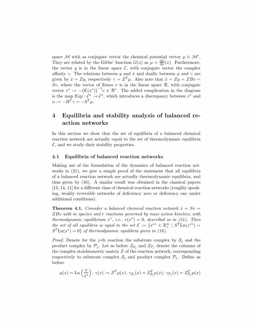
Making use of the formulation of the dynamics of balanced reaction net-works in (21), we give a simple proof of the statement that all equilibriaof a balanced reaction network are actually thermodynamic equilibria, andthus given by (16). A similar result was obtained in the classical papers[13, 14, 11] for a different class of chemical reaction networks (roughly speak-ing, weakly reversible networks of deficiency zero or deficiency one underadditional conditions).

Theorem 4.1. Consider a balanced chemical reaction network x = Sv =ZBv with m species and r reactions governed by mass action kinetics, withthermodynamic equilibrium x∗, i.e., v(x∗) = 0, described as in (21). Thenthe set of all equilibria is equal to the set E := {x∗∗ ∈ R

m+ | S

TLn(x∗∗) =STLn(x∗) = 0} of thermodynamic equilibria given in (16).

Proof. Denote for the j-th reaction the substrate complex by Sj and theproduct complex by Pj. Let as before ZSj

and ZPjdenote the columns of

the complex stoichiometric matrix Z of the reaction network, correspondingrespectively to substrate complex Sj and product complex Pj . Define asbefore

µ(x) = Ln( x

x∗

)

, γ(x) := ZTµ(x), γSj(x) = ZT

Sjµ(x), γPj

(x) = ZTPjµ(x)

Suppose x∗∗ is an equilibrium, i.e., ZBK(x∗)BTExp(

ZTLn(

x∗∗

x∗

))

= 0, orequivalently ZBK(x∗)BTExp

(

ZTµ(x∗∗))

= 0. Then also

µT (x∗∗)ZBK(x∗)BTExp(

ZTµ(x∗∗))

= 0

Denoting the columns of B by b1, · · · , br, we have

BK(x∗)BT =

r∑

j=1

κj(x∗)bjb

Tj

while

µT (x∗∗)Zbj = µT (x∗∗)(

ZPj− ZSj

)

= γTPj(x∗∗)− γTSj

(x∗∗),

bTj Exp(

ZTµ(x∗∗))

= exp(

γTPj(x∗∗)

)

− exp(

γTSj(x∗∗)

)

It follows that

0 = µT (x∗∗)ZBK(x∗)BTExp(

ZTµ(x∗∗))

=∑r

j=1

[

γPj(x∗∗)− γSj

(x∗∗)] [

exp(

γPj(x∗∗)

)

− exp(

γSj(x∗∗)

)]

κj(x∗)

Since the exponential function is a strictly increasing function and κj(x∗) >

0, j = 1, · · · , r, this implies that all terms in the summation are zero andthus

γPj(x∗∗) = γSj

(x∗∗), j = 1, · · · , r

exp(

γPj(x∗∗)

)

= exp(

γSj(x∗∗)

)

, j = 1, · · · , r

which is equivalent to

BTγ(x∗∗) = BTZTµ(x∗∗) = 0, BTExp (γ(x∗∗)) = BTExp(

ZTµ(x∗∗))

= 0

The first equality tells us that x∗∗ ∈ E , and thus a thermodynamical equi-librium (as also follows from the second equality). �

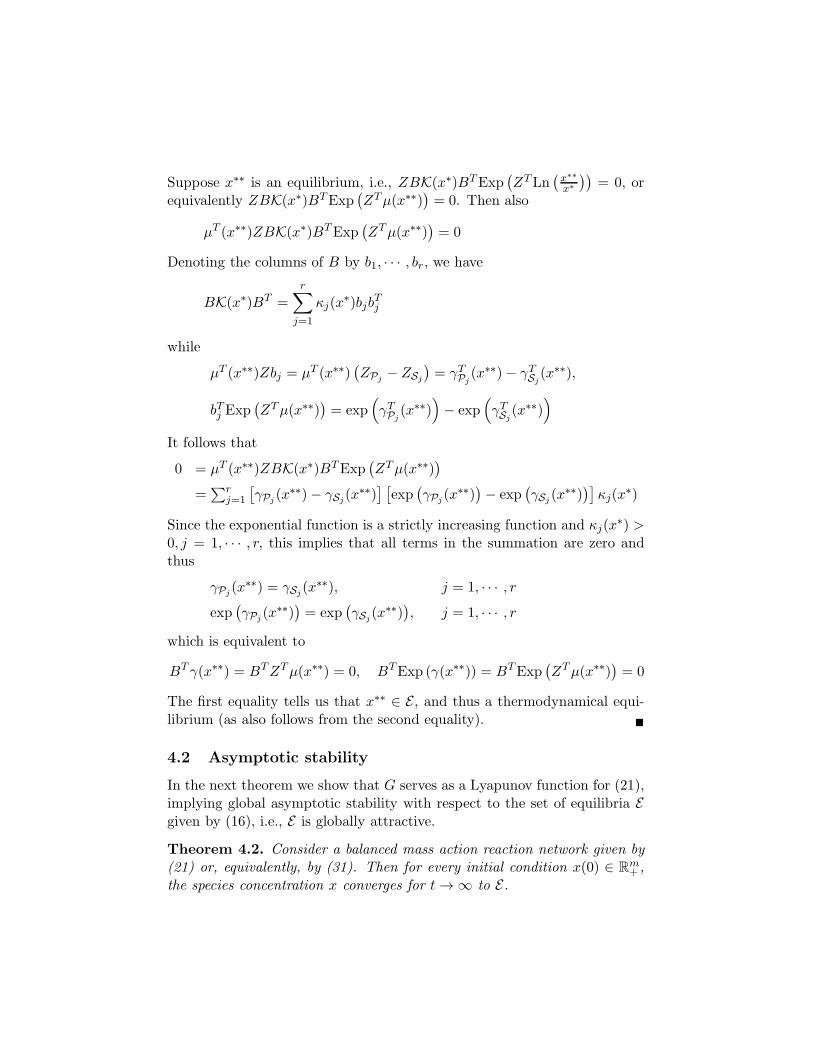
4.2 Asymptotic stability

In the next theorem we show that G serves as a Lyapunov function for (21),implying global asymptotic stability with respect to the set of equilibria Egiven by (16), i.e., E is globally attractive.

Theorem 4.2. Consider a balanced mass action reaction network given by(21) or, equivalently, by (31). Then for every initial condition x(0) ∈ R

m+ ,

the species concentration x converges for t→∞ to E.

Proof. First we prove that the function G in (30) satisfies

G(x∗) = 0, G(x) > 0, ∀x 6= x∗, (33)

and is proper, i.e., for every real c > 0 the set {x ∈ Rm+ | G(x) ≤ c} is

compact. With regard to (33) we first note the following. Let xi and x∗idenote the i-th elements of x and x∗ respectively. From the strict concavityof the logarithmic function

z − 1 ≥ ln(z), ∀z ∈ R+, (34)

with equality if and only if z = 1. Putting z =x∗i

xiin equation (34), we get

x∗i − xi + xi ln

(

xix∗i

)

≥ 0,

with equality if and only if xi = x∗i . This implies that

G(x) =

m∑

i=1

[

x∗i − xi + xi ln

(

xix∗i

)]

≥ 0,

with equality if and only if xi = x∗i , i = 1, · · · ,m. Thus G has a strictminimum at x = x∗ and satisfies (33). Properness of G is readily checked.

Next we will show that G(x) := ∂TG∂x

(x)Sv(x) = dGdt(x) satisfies

G(x) ≤ 0 ∀x ∈ Rm+ , (35)

and

G(x) = 0 if and only if x ∈ E . (36)

As in the proof of Theorem 4.1, let the j-th reaction be between substratecomplex Sj and product complex Pj , and let ZSj

and ZPjdenote the columns

of the complex stoichiometric matrix Z corresponding to complexes Sj andPj . Define as before

µ(x) = Ln( x

x∗

)

, γ(x) := ZTµ(x), γSj(x) = ZT

Sjµ(x), γPj

(x) = ZTPjµ(x)

Then compute12

G(x) = ∂TG∂x

(x)x = −µT (x)ZBK(x∗)BTExp(ZTµ(x))

= −γT (x)BK(x∗)BTExp(γ(x))

=∑r

j=1

[

γPj(x)− γSj

(x)] [

exp(

γPj(x)

)

− exp(

γSj(x)

)]

κj(x∗)

≤ 0 ,

12See the proof of Theorem 4.1 for an analogous reasoning.

(37)

since κj(x∗) > 0 for j = 1, . . . , r, and the exponential function is strictly

increasing. The “if” part in (36) is trivial. For the “only if” part, thesummand in the third line of (37) is zero only if γSj

(x) − γPj(x) = 0 for

every j. This is equivalent to having BTγ(x) = 0. Thus, G(x) = 0 only ifBTγ = BTZTLn

(

xx∗

)

= 0. It follows that G(x) = 0 if and only if x ∈ E .Suppose that the set R

m+ is not forward invariant with respect to (31),

and that xi(t) = 0 for some t and i ∈ {1, · · · ,m}. Without loss of gen-erality assume that the species with concentration xi is taking part in atleast one complex which is involved in a reaction. Let Ci denote the sub-set of complexes which contain xi, i.e., Zi,Ci 6= 0. Then it follows thatExp(ZT

Ciµ(x(t))) = 0 and thus

xi(t) = −ZiBK(x∗)BTExp(ZTµ(x)) > 0,

where Zi is the i-th row vector of Z. This inequality is due to the factthat the terms corresponding to the positive i-th diagonal element of theweighted Laplacian matrix BK(x∗)BT are all zero, while there is at leastone term corresponding to a non-zero, and therefore strictly negative, off-diagonal element of BK(x∗)BT . This implies13 that R

m+ must be forward

invariant.Since G is proper (in R

m+ ) and the state trajectory x(·) remains in R

m+ ,

(35) implies that x(·) is bounded in Rm+ . Therefore, boundedness of x(·),

together with equations (35) and (36), imply that the species concentrationx converges to E by an application of LaSalle’s invariance principle. �

Remark 4.3. A similar reasoning for showing that G ≤ 0 was used in [2],see also [13, 10, 11]; however making use of the convexity of the exponen-tial function instead of the weaker property that the exponential function isincreasing as in our proof. In this respect, it can be noted that Theorem 4.2remains unaltered if we replace the dynamics (21) by any equations of theform (not corresponding anymore to mass action kinetics)

x = −ZBK(x∗)BTF(

ZTLn( x

x∗

))

,

with F : Rc → Rc a mapping F (y1, · · · , yc) = diag(f1(y1), · · · , fc(yc)), where

the functions fi, i = 1, · · · , c, are all monotonously increasing.

13A similar argument can be used directly for the mass action kinetics rate equations.

4.3 Equilibrium concentration corresponding to an initial

concentration

In this section, we show that for every initial concentration vector x0 ∈Rm+ , the solution trajectory of (21) converges to a unique thermodynamic

equilibrium in E . Our reasoning is very similar to the proof of zero-deficiencytheorem provided in [11] and is based on the following proposition in there.Recall from the Introduction that the product x · z ∈ R

m is defined as theelement-wise product (x · z)i = xizi, i = 1, · · · ,m.

Proposition 4.4. Let U be a linear subspace of Rm, and let x∗, x0 ∈ Rm+ .

Then there is a unique element µ ∈ U⊥, such that(

x∗ · Exp(µ)− x0)

∈ U .

Proof. See proof of [11, Proposition B.1, pp. 361-363]. �

Theorem 4.5. Consider the balanced chemical reaction network (21). Thenfor every x0 ∈ R

m+ , there exists a unique x1 ∈ E such that the solution

trajectory of (21) starting from x0 converges for t→∞ to x1. Hence thereexists a surjective map χ : Rm

+ → E that assigns to every initial state itsasymptotic thermodynamic equilibrium14.

Proof. With reference to Proposition 4.4, define U = spanS, and observethat U⊥ = kerST . Let x∗, x0 ∈ R

m+ . Then by Proposition 4.4, there exists

a unique µ ∈ kerST such that x∗ · Exp(µ) − x0 ∈ spanS. Define x1 :=x∗ · Exp(µ) ∈ R

m+ . It follows that STµ = STLn

(

x1

x∗

)

= 0, i.e., x1 ∈ E . Also,since x1−x0 ∈ spanS, x1 ∈ {ξ ∈ R

m | ξ−x0 ∈ spanS} which is an invariantset of the dynamics. Together with Theorem 4.2, the state trajectory withinitial condition x0 converges to the unique equilibrium x1 ∈ E . �

4.4 Relation with consensus dynamics

The form of the equations (10) is reminiscent of consensus dynamics formulti-agent systems with non-symmetric communication. In fact, a stan-dard consensus algorithm in the vector y ∈ R

c can be written as [17]

y = −Lconsy,

where Lcons is the weighted Laplacian matrix of the communication graph.This weighted Laplacian is constructed similarly as in (9), with the differ-ence that ∆ is now defined as the diagonal matrix whose (ρ, ρ)-th element

14The map χ is an analytic function, following a similar argument as used in [23, The-orem 6] which deals with weakly-reversible zero-deficiency chemical networks.

is equal to the sum of the elements of the ρ-th row of A, implying that thesum of the elements of every row of Lcons is zero. Note that in contrast forthe weighted Laplacian L in (9) the sum of the elements of every column iszero15. Seen from this perspective, the equations (21) for balanced chemi-cal reaction networks, exhibiting the symmetric weighted Laplacian matrixBK(x∗)BT , correspond to the consensus algorithm for multi-agent systemswith symmetric communication structure [17].

Finally, Theorem 4.5 is closely related to the property that the asymp-totic consensus value in consensus dynamics is a function of the initial state.In fact, the surjective map χ : Rm

+ → E which assigns to every initial stateits asymptotic equilibrium is similar to the χ-function in the χ-consensusalgorithm of [5].

5 Chemical reaction networks with boundary fluxes

and interconnection of reaction networks

As discussed in Section 2.1, the interaction of a chemical reaction networkwith the environment or another chemical reaction network can be modeledby identifying a vector of boundary chemical species xb ∈ R

b, which is a sub-vector of the vector x of concentrations of all the chemical species in thenetwork. These boundary chemical species are the species that are subjectto inflow or outflow boundary fluxes vb. The natural conjugate vector is (upto the constant RT ) the vector of chemical potentials µb = ST

b µ ∈ Rb of

boundary potentials. Indeed, up to the factor RT , the product µTb vb is equal

to the power entering or leaving the chemical reaction network due to theinflux or efflux of boundary chemical species.

By combining (3) and (21) this leads to the following equations

x = −ZBK(x∗)BTExp(

ZTLn(

xx∗

))

+ Sbvb,

µb = STb Ln

(

xx∗

)

,(38)

which define an input-state-output system with inputs16 vb and outputs µb.Let G be defined by equation (30). Define as before γ(x) := Z⊤Ln

(

xx∗

)

. As

15Of course, another main difference between the two dynamics is the appearance ofthe complex stoichiometric matrix Z on the left of the right-hand side of the differentialequation (10), and the much more involved term Exp

(

ZTLn(x))

instead of simply y (seehowever [5]).

16Note however that the elements of vb can be either inflows or outflows for the network.

an immediate consequence we obtain the following energy balance

d

dtG(x) = −γT (x)BK(x∗)BTExp(γ(x)) + µT

b vb (39)

Furthermore, since the exponential function is increasing it is easily verifiedalong the lines of the proof of Theorem 4.2

(

see in particular (37))

, thatγTKBTExp(γ) ≥ 0, thus showing the passivity property

d

dtG ≤ µT

b vb (40)

5.1 Interconnection of chemical reaction networks

The most basic way of interconnecting chemical reaction networks is throughshared boundary chemical species. Consider for simplicity of notation the in-terconnection of two chemical reaction networks which have all their bound-ary chemical species in common; the generalization to the general case isstraightforward. Let Bi denote the incidence matrix of the complex graph,and Zi the complex stoichiometry matrix of network i = 1, 2. The complexgraph of the interconnected chemical reaction network is the direct union ofthe complex graphs of networks 1 and 2, with incidence matrix B given asthe direct product

B =

[

B1 00 B2

]

(41)

Note that the complex graph of such an interconnected network is not con-nected. In fact, if all the constituent networks are connected then theircomplex graphs are linkage classes of the interconnected network, cf. Sec-tion 3.4.

The complex stoichiometry matrix of the interconnected network is moreinvolved. Permute the chemical species x1, x2 such that

x1 = (x1, xb1), x2 = (xb2, x2), Z1 =

[

Z1

Zb1

]

, Z2 =

[

Zb2

Z2

]

,

where Zb1, Zb2 are matrices with the same number of rows, equal to thenumber of shared boundary species

xb := xb1 = xb2 ∈ Rb

Then the stoichiometry matrix Z of the interconnected network is given as

Z =

Z1 0Zb1 Zb2

0 Z2

(42)

Note that in general the property of zero-deficiency is not maintained underinterconnection. In fact, this was already discussed in Proposition 3.8 inSection 3.4 following [21].

Remark 5.1. It may occur that one or more columns of the matrix Z in(42) are actually the same, corresponding to the case that the two reac-tion networks have shared complexes (by definition only consisting of sharedboundary chemical species; i.e., for which the corresponding columns of Z1

and Z2 are zero). Then one may identify the equal columns in the matrix Z,and thus obtain a reduced network with complex graph consisting of the unionof the complex graphs of the two networks with the vertices corresponding tothe shared complexes being identified. In this case the complex graph of theinterconnected network may still be connected.

The property of ’balancedness’ is not necessarily maintained under inter-connection. Sufficient conditions for this to happen are given in the followingproposition.

Proposition 5.2. The interconnection of two balanced reaction networkswith vectors of equilibrium constants Keq

1 ,Keq2 is again balanced if and only

if there exists (x∗∗1 , x∗∗2 , x∗∗b ) such that

Ln

([

Keq1

Keq2

])

=

[

BT1 Z

T1 0 BT

1 ZTb1

0 BT2 Z

T2 BT

2 ZTb2

]

Ln

x∗∗1x∗∗2x∗∗b

(43)

There exists such a thermodynamic equilibrium for the interconnected net-work if there is a partition {1, · · · , b} = I1

⋃

I2 such that all columns ofBT

1 ZTb1 corresponding to the index set I1 are contained in the image of BT

1 ZT1 ,

and all columns of BT2 Z

Tb2 corresponding to the complementary index set I2

are contained in the image of BT2 Z

T2 .

Proof. By assumption there exist thermodynamic equilibrium points (x∗1, x∗b1)

and (x∗b2, x∗2) of the two individual networks. That means (cf. 14)) that

Ln(Keq1) = B1

[

ZT1 ZT

b1

]

Ln

([

x∗1x∗b1

])

(44)

Ln(Keq2 ) = B2

[

ZT2 ZT

b2

]

Ln

([

x∗2x∗b2

])

(45)

Now define x∗∗b ∈ Rb by taking its i-th component for i ∈ I1 equal to the

i-th component of x∗b2, and for i ∈ I2 equal to the i-th component of x∗b1.Then there exist corresponding x∗∗1 , x∗∗2 such that (43) is satisfied. �

Under the assumptions of Proposition 5.2) it follows that the balancedinterconnected network is given as

˙x1˙x2xb

= −ZB

[

K1(x∗∗1 , x∗∗b ) 00 K2(x

∗∗2 , x∗∗b )

]

BTExp

ZTLn

x1/x∗∗1

x2/x∗∗2

xb/x∗∗b

,

(46)

where B as in (41), Z as in (42), x∗∗1 , x∗∗2 , x∗∗b satisfy (43), and K1(x∗∗1 , x∗∗b )

and K2(x∗∗2 , x∗∗b ) are proportionally related to K1(x

∗1, x

∗1b) and K2(x

∗2, x

∗2b),

respectively, as follows from Proposition 3.6.

5.2 Interconnection arising from port interconnection

The above procedure for interconnection of chemical reaction networks canbe also interpreted as arising from power-port interconnection at the bound-ary chemical species. Recall the formulation (38) of an open chemical reac-tion network with inputs vb being the influx/efflux of the boundary chemicalspecies and µb their chemical potentials. Then the interconnection of twochemical reaction networks (as above under the simplifying assumption thatall boundary chemical species are shared) can be seen to result from thepower-port interconnection constraints

µb1 = µb2, vb1 + vb2 = 0, (47)

expressing that the chemical potentials of the boundary chemical species areequal, while the boundary fluxes of the two networks add up to zero (conser-vation of boundary chemical species). Indeed, the resulting interconnecteddynamics given by the differential-algebraic equations

[

x1

x2

]

= −

[

−Z1B1K1(x∗1)B

T1 Exp(Z

T1 µ1(x1))

Z2B2K2(x∗2)B

T2 Exp(Z

T2 µ2(x2))

]

+

[

I

−I

]

v

0 =[

I −I]

[

µb1(x1)

µb2(x2)

]

with v = vb1 = −vb2 acting as a vector of Lagrange multipliers, can beseen, after elimination of the algebraic constraint µb1(x1) = µb2(x2) and theLagrangian multipliers v, to result in the dynamics

x = −ZBK(x∗1, x∗2)B

TExp(ZTµ(x1, x2))

where x = (x1, x2, xb) denotes the total vector of chemical species (internalspecies of both networks, together with the shared boundary species). Herethe complex stoichiometric matrix Z and incidence matrix B of the intercon-nected network are as above, and where K(x∗1, x

∗2) = diag(K1(x

∗1),K2(x

∗2))

and µ(x1, x2) =

[

µ1(x1)µ2(x2)

]

. Recalling that µTb vb is (modulo the constant RT )

the power provided to the chemical reaction network, this implies that theinterconnection (47) is power-preserving, that is µT

b1vb1 + µTb2vb2 = 0, in line

with the standard way of interconnecting physical networks [19, 18, 20].

6 Model reduction of chemical reaction networks

For many purposes one may wish to reduce the number of dynamical equa-tions of a complex chemical reaction network in such a way that the behaviorof a number of key chemical species is approximated in a satisfactory way.

Furthermore, it is important that the reduced system again allows theinterpretation of a chemical reaction network (but with much less chemi-cal species involved). In fact, most of the approaches to model reductionof large-scale chemical reaction networks aim at doing exactly this: theysimplify the pathways of the chemical reaction network by leaving out in-termediate species or complexes; see e.g. [9, 1], or the standard reduction ofmass action enzymatic reactions to their Michaelis-Menten description [15].

In the following we will propose a model reduction approach which isbased on a reduction of the complex graph. First we recall from [22] the fol-lowing result regarding Schur complements of weighted Laplacian matrices.

Proposition 6.1. Consider a directed graph with vertex set V and withweighted Laplacian matrix L = BK(x∗)BT . Then the Schur complementwith respect to any subset of vertices Vr ⊂ V is well-defined, and is theweighted Laplacian matrix L = BK(x∗)BT of a reduced directed graph withincidence matrix B whose vertex set is equal to V − Vr.

Remark 6.2. Note that the reduced graph defined by B may contain ad-ditional edges between the remaining vertices in V − Vr. Furthermore, theweights of the reduced diagonal weight matrix K(x∗) are in general differentfrom the weights of the original weight matrix K(x∗), and represent equiva-lent balanced reaction constants17.

17In electrical circuit theory the process of reduction of a resistive network to a resistivenetwork with fewer vertices but equivalence resistance is sometimes referred to as Kron

reduction, cf. [16, 8].

This result can be directly applied to the complex graph, yielding areduction of the chemical reaction network by reducing the number of com-plexes. The procedure is as follows. Consider a balanced reaction networkdescribed in the standard form (21)

Σ : x = −ZBK(x∗)BTExp(

ZTLn( x

x∗

))

Reduction will be performed by deleting certain complexes in the com-plex graph, resulting in a reduced complex graph with weighted LaplacianL = BK(x∗)BT . Furthermore, leaving out the corresponding columns ofthe complex stoichiometric matrix Z one obtains a reduced complex stoi-chiometric matrix Z (with as many columns as the remaining number ofcomplexes in the complex graph), leading to the reduced reaction network

Σ : x = −ZBK(x∗)BTExp(

ZTLn( x

x∗

))

, K(x∗) > 0 (48)

Note that Σ is again a balanced chemical reaction network governed by massaction kinetics, with a reduced number of complexes and with, in general,a different set of reactions (edges of the complex graph). Note furthermorethat the thermodynamic equilibrium x∗ of the original reaction network Σis a thermodynamic equilibrium of the reduced network Σ as well.

Furthermore, we can derive the following properties relating Σ and Σ.

Proposition 6.3. Consider the balanced reaction network Σ and its reducedorder model Σ given by (48). Denote their sets of equilibria by E, respectivelyE. Then E ⊂ E . Furthermore, if Σ has deficiency zero then so does Σ.

Proof. Assume that the complex graph is connected; otherwise the sameargument can be repeated for every component (linkage class). Recall from(16) that the set of equilibria E is given as {x∗∗ | LnT (x∗∗)S = LnT (x∗)S},where S = ZB. It follows that E is equivalently represented as

E = {x∗∗ | LnT (x∗∗)ZL = LnT (x∗)ZL},

where L := BK(x∗)BT is the weighted Laplacian matrix of the complexgraph. Now consider a subset Vr of the set of all complexes, which we wishto leave out in the reduced network. After permutation of the complexes wepartition L and Z correspondingly as

L =

[

L11 L12

L21 L22

]

, Z =[

Z1 Z2

]

where Vr corresponds to the last part of the vertices. Then post-multiplythe equations LnT (x∗∗)ZL = LnT (x∗)ZL by the invertible matrix

[

I 0

−L−122 L21 I

]

, (49)

not changing the solution set E . It follows that

E = {x∗∗ | LnT (x∗∗)[

Z1 Z2

]

[

L11 − L12L−122 L21 L12

0 L22

]

=

LnT (x∗)[

Z1 Z2

]

[

L11 − L12L−122 L21 L12

0 L22

]

}

⊂ {x∗∗ | LnT (x∗∗)ZL = LnT (x∗)ZL} = E ,

since Z = Z1 and L = L11 − L12L−122 L21.

For the second statement assume that the full-order network has defi-ciency zero, i.e., kerZ

⋂

imB = 0, or equivalently kerZ⋂

imL = 0. Post-multiplication of L with the matrix in (49) yields

ker[

Z1 Z2

]

⋂

im

[

L11 − L12L−122 L21 L12

0 L22

]

= 0,

which implies ker Z⋂

im L = 0, i.e., zero-deficiency of the reduced-ordernetwork Σ. �

The precise properties of this model reduction approach are currentlyunder investigation. At least the approach seems to have favorable prop-erties for the shortening of linear pathways, leaving out the intermediarycomplexes. Furthermore, in most cases it seems natural not to leave outcomplexes containing boundary chemical species. Note that the model re-duction approach results in the reduction of a number of chemical species inthe reduced network once these chemical species are only contained in thecomplexes that are deleted in the reduction procedure.

6.1 Reversible enzymatic reaction

As a very simple example, let us apply the above procedure to a standardreversible enzymatic reaction represented as

E +X ⇋ I ⇋ E + Y ,

where X,Y denote chemical species, E the enzyme, and I the intermediatespecies (or complex). The three complexes involved are E + X, I,E + Yand we want to leave out the intermediate complex I. Since the transposedstoichiometric matrix ST has full row-rank the Wegscheider conditions (15)are trivially satisfied, guaranteeing the existence of a thermodynamic equi-librium. Denote for later use the concentrations of the species X,Y,E byx, y, e, and their thermodynamic equilibrium concentrations by x∗, y∗, e∗.

Furthermore, denote the balanced reaction constant of the first reversiblereaction by κX , and of the second one by κY . Then the weighted Laplacianmatrix of the complex graph is given by

L =

κX −κX 0−κX κX + κY −κY0 −κY κY

Deletion of the intermediate complex I corresponds to taking the Schurcomplement of L with respect to the second row and column, yielding thereduced weighted Laplacian matrix

L =

[

κ −κ−κ κ

]

,

where the reduced balanced reaction constant κ is computed as

κ :=κXκY

κX + κY

Furthermore, the reduced complex stoichiometric matrix Z expressing theremaining complexes E +X,E + Y in terms of the species X,Y,E is givenby18

Z =

1 00 11 1

It follows that the reduced dynamics (48) is given as

xye

= −

1 00 11 1

[

κ −κ−κ κ

]

Exp

[

1 0 10 1 1

]

ln(

xx∗

)

ln(

yy∗

)

ln(

ee∗

)

=

−110

(

κe∗x∗ ex−

κe∗y∗

ey)

,

18Strictly speaking, the matrix Z should be complemented by a zero row correspond-ing to the chemical species I , which is however not present anymore in the remainingcomplexes.

which is in mass action kinetics form, and has (x∗, y∗, e∗) as a thermo-dynamic equilibrium. Note that in the reduced model the total enzymeconcentration e is preserved (as to be expected).

It is easily checked that the equations for the x, y and e values of thethermodynamic equilibria of the reduced network are the same as for theoriginal network. On the other hand, in contrast with the thermodynamicequilibrium equations for i of the original model, the reduced model allowsany value of i as equilibrium value; in accordance with Proposition 6.3.Furthermore, both networks are trivially zero-deficient.

7 Conclusions

In this paper we have provided a compact, geometric, formulation of thedynamics of mass action chemical reaction networks possessing a thermo-dynamic equilibrium. This formulation clearly exhibits both the structureof the complex graph and the stoichiometry, and furthermore admits a di-rect thermodynamical interpretation. Exploiting this formulation we wereable to recover, for this subclass of mass action kinetics chemical reactionnetworks, some of the results in the fundamental work [14, 13, 10, 11] in asimple and insightful way, without having to rely on the properties of defi-ciency zero or one. Drawing inspiration from [19, 18, 20], we have shown howthe framework leads to an input-state-output formulation of open chemicalreaction networks, and how this may be used for interconnection. Further-more, we have indicated how this formulation, in particular its emphasis onthe Laplacian matrix of the complex graph, may be used for a systematicmodel reduction procedure based on the elimination of certain intermediatecomplexes.

Current research is taking place in a number of directions. We believe thestriking similarity with consensus dynamics can be further exploited. Also,the use of our formulation for the analysis of steady states corresponding tonon-zero (constant) boundary fluxes is under study, taking into account thepossibility of multiple steady states [6]; see also the work [4] on input-outputstability. The ramifications of the new model reduction procedure are beinginvestigated, including the comparison with classical reduction schemes like(reversible) Michaelis-Menten reaction rates; see e.g. [15]. Furthermore, theLaplacian matrix can not only be used for model reduction, but also forother analysis purposes of the complex graph, e.g. for its decompostion [1].Finally, a challenging question is the extension to biochemical reaction net-works, where the reactions are mostly enzymatic reactions, and the amount

of enzymes, through the activity of the gene and protein networks, willdepend on e.g. the concentration of a number of chemical species (metabo-lites). This will lead to the introduction of an additional network structureoriginating from the regulatory, and possibly competing, feedback loops.

References

[1] J. Anderson, Y.-C. Chang, A. Papachristodoulou, ”Model decomposi-tion and reduction tools for large-scale networks in systems biology”,Automatica, 47, pp. 1165–1174, 2011.

[2] D. Angeli, ”A tutorial on chemical reaction network dynamics”, Euro-pean Journal of Control, 15 (3-4), pp. 398–406, 2009.

[3] B. Bollobas, Modern Graph Theory, Graduate Texts in Mathematics184, Springer, New York, 1998.

[4] M. Chaves, ”Input-to-state stability of rate-controlled biochemical re-action networks”, SIAM J. Control Optim., 44(2), pp. 704–727, 2005.

[5] J. Cortes, “Distributed algorithms for reaching consensus on generalfunctions,” Automatica, vol. 44, no. 3, pp. 726-737, 2008.

[6] G. Craciun, M. Feinberg, “Multiple equilibria in complex chemical re-action networks: I. the injectivity property”, SIAM J. Appl. Math.,65(5), pp. 1526–1546, 2006.

[7] P. De Leenheer, E. Sontag, D. Angeli, “A Petri net approach to thestudy of persistence in chemical reaction networks, Mathematical Bio-sciences, 210, pp.: 598 - 618, 2007.

[8] F. Dorfler, F. Bullo, ”Synchronization of power networks: Networkreduction and effective resistance”, in IFAC Workshop on DistributedEstimation and Control in Networked Systems, Annecy, France, Sept.2010, pp. 197202.

[9] G. Farkas, ”Kinetic lumping schemes”, Chem. Eng. Sci., 54, pp. 3909–3915, 1999.

[10] M. Feinberg, “Chemical reaction network structure and the stabilityof complex isothermal reactors -I. The deficiency zero and deficiencyone theorems”, Chemical Engineering Science, 43(10), pp. 2229–2268,1987.

[11] M. Feinberg, “The existence and uniqueness of steady states for a classof chemical reaction networks”, Arch. Rational Mech. Anal., 132, pp.311–370, 1995.

[12] M. Feinberg, “Necessary and sufficient conditions for detailed balancingin mass action systems of arbitrary complexity”, Chemical EngineeringScience, 44(9), pp. 1819–1827, 1989.

[13] F.J.M. Horn, ”Necessary and suffcient conditions for complex balanc-ing in chemical kinetics”, Arch. Rational Mech. Anal., 49, pp. 172–186,1972.

[14] F.J.M. Horn, R. Jackson, “General mass action kinetics”, Arch. Ratio-nal Mech. Anal., 47, pp. 81–116, 1972.

[15] E. Klipp, W. Liebermeister, C. Wierling, A. Kowald, H. Lehrach, R.Herwig, Systems Biology, Wiley-Blackwell, Weinheim, Germany, 2009.

[16] G. Kron, Tensor Analysis of Networks, Wiley, 1939.

[17] R. Olfati-Saber, J.A. Fax, R.M. Murray, “Consensus and cooperationin networked multi-agent systems”, Proceedings of the IEEE, 95, No.1,2007.

[18] J.F. Oster, A.S. Perelson, A. Katchalsky, “Network dynamics: dynamicmodeling of biophysical systems”, Quarterly Reviews of Biophysics,6(1), pp. 1-134, 1973.

[19] J.F. Oster, A.S. Perelson, “Chemical reaction dynamics, Part I: Geo-metrical structure”, Archive for Rational Mechanics and Analysis, 55,pp. 230-273, 1974.

[20] J.F. Oster, A.S. Perelson, ””Chemical reaction networks”, IEEE Cir-cuits Syst. mag, 21(6), pp. 709–721, 1974.

[21] H. G. Othmer, Analysis of Complex Reaction Networks, Lecture Notes,School of Mathematics, University of Minnesota, December 9, 2003.

[22] A.J. van der Schaft, “Characterization and partial synthesis of thebehavior of resistive circuits at their terminals”, Systems & ControlLetters, 59, pp. 423–428, 2010.

[23] E.D. Sontag, ”Structure and stability of certain chemical networks andapplications to the kinetic proofreading model of T-cell receptor signal

transduction”, IEEE Trans. Autom. Control, 46(7), pp. 1028–1047,2001.

[24] R. Wegscheider, ”Uber simultane Gleichgewichte und die Beziehungenzwischen Thermodynamik und Reaktionskinetik homogener Systeme”,Zetschrift fur Physikalische Chemie, pp. 257–303, 1902.