NBER WORKING PAPER SERIES

ON THE LINK BETWEEN THE VOLATILITY AND SKEWNESS OF GROWTH

Geert BekaertAlexander Popov

Working Paper 18556http://www.nber.org/papers/w18556

NATIONAL BUREAU OF ECONOMIC RESEARCH1050 Massachusetts Avenue

Cambridge, MA 02138November 2012

We thank George-Marios Angeletos, Markus Brunnermeier, Francis Diebold, Simon Gilchrist, FrancoisGourio, Bartozs Mackowiak, Kalin Nikolov, and Philippe Weil, as well as seminar participants atthe ECB, for useful discussions. The views expressed do not necessarily reflect those of the EuropeanCentral Bank, the Eurosystem, or the National Bureau of Economic Research.

NBER working papers are circulated for discussion and comment purposes. They have not been peer-reviewed or been subject to the review by the NBER Board of Directors that accompanies officialNBER publications.

© 2012 by Geert Bekaert and Alexander Popov. All rights reserved. Short sections of text, not to exceedtwo paragraphs, may be quoted without explicit permission provided that full credit, including © notice,is given to the source.

On the Link Between the Volatility and Skewness of GrowthGeert Bekaert and Alexander PopovNBER Working Paper No. 18556November 2012, Revised December 2013JEL No. E32,G10,O10

ABSTRACT

In a sample of 110 countries over the period 1960-2009, we document a positive relation betweenthe volatility and skewness of growth in the cross-section. The relation holds regardless of initial levelof economic development and of subsequent long-run growth rate. We argue that this novel stylizedfact is related to two distinct phenomena: sudden growth spurts in mostly emerging markets, and rareand abrupt crises in mostly developed economies. The former phenomenon is driven by industrialization,macroeconomic stabilization, and the exploitation of natural resources. The latter is consistent withrecent theories of financial frictions. The positive relation between volatility and skewness in the cross-sectionis in sharp contrast with a negative relation between the two in panel data with country fixed effectswhich is fully driven by business cycle variation in rich countries.

Geert BekaertGraduate School of BusinessColumbia University3022 Broadway, 411 Uris HallNew York, NY 10027and NBERgb241@columbia.edu

Alexander PopovEuropean Central BankAlexander.Popov@ecb.int

1

I. Introduction

This paper documents a novel stylized fact: in a large cross-section of countries, the

volatility and the skewness of GDP growth are positively correlated over the long run. As a

concrete example, countries in the highest decile in terms of volatility1 exhibit an average

skewness over the 1960-2009 period of 1.51, while the lowest volatility decile exhibits an

average skewness of -0.71. The statistical association between volatility and skewness is

significant and robust to the removal of outliers. It is also robust to sample selection; for

example, it holds for the top and bottom quartile of countries both in terms of 1960 per capita

GDP and in terms of subsequent average long-run growth rates.

This stylized fact regarding the relation between the volatility and skewness of output

growth is not easily reconciled with the predictions of a variety of macro-economic and

development models. For a start, it appears inconsistent with the temporal negative relationship

predicted by the business cycle literature. A large number of papers have empirically established

that business cycles are negatively skewed, with recessions occurring suddenly and being sharp,

whereas booms occur more slowly (see, e.g., Neftci, 1984; Diebold and Rudebusch, 1990;

Hamilton, 1989; Sichel, 1993; and Acemoglu and Scott, 1994). These data features naturally

suggest a temporal negative link between volatility and skewness. Models explaining this type of

behaviour include, for example, Acemoglu and Scott (1997), who relate the business cycle

asymmetry to intertemporal increasing returns to investment, and Zeira (1994), Jovanovic

(2003), and Van Nieuwerburgh and Veldkamp (2006), whose models rely on a learning process

in which either bad signals are more extreme than good signals, or signals are less noisy during

booms. Given the recent interest in differences between business cycles in emerging markets and

developed countries (see e.g. Aguiar and Gopinath, 2007; Garcia-Cicco, Pancrazi, and Uribe,

2010), an interesting question is whether this stylized fact is universal or restricted to the

developed countries for which it has hitherto been documented. We show that in panel data with

country fixed effects, volatility and skewness are indeed temporally negatively correlated.

However, this is fully driven by business cycle variation in industrialized economies. In 1 While in the empirical tests we employ the natural logarithm of the standard deviation of GDP growth, in the text we interchangeably refer to the “volatility” of GDP growth.

2

particular, the relation between volatility and skewness starts to be negative from a GDP per

capita level of $1231 in 2005 dollars, and is only significant for very rich (mostly industrialized

OECD) countries. Hence, development comes with a very unattractive business cycle pattern,

where low growth periods go hand in hand with high real volatility.

Importantly, business cycle models suggest that the mechanisms which generate business

cycle asymmetry are hardwired in the business cycle itself and do not depend on the size of the

volatility-generating shocks. This also applies to the new generation growth-business cycle

model of Comin and Gertler (2006) which uses technological change to generate medium-

frequency oscillations between periods of robust growth and periods of relative stagnation. In

short, business cycle models do not offer a mechanism for the positive cross-sectional

relationship between volatility and skewness observed in the data.

The stylized fact is not fully captured in various development and growth models, either.

For example, Acemoglu and Zilibotti (1997) suggest that under-developed countries, likely

prevalent in our sample, are stuck in an equilibrium with high output variability as indivisibilities

in the production process limits the economy’s ability to diversify idiosyncratic risk. Only when

they experience “lucky draws” do they accumulate enough capital to invest in large indivisible

high-growth projects, at which point the economy takes off and volatility declines due to

diversification. Furthermore, Acemoglu et al. (2003) identify institutions as the key determinant

of the mean and variability of the growth process, and suggest that better institutions come with

higher growth, lower volatility, and less severe contractions. This would suggest a negative

cross-sectional relationship between skewness and volatility. However, we show that the positive

cross-sectional relationship we observe holds for all development levels. The recent theoretical

literature that models regime switching as part of a unified growth theory provides a different

endogenous mechanism for a transition from a “Malthusian” equilibrium (low economic growth

and high population growth) to a “Solowian” equilibrium (high economic growth and low

population growth), one based on human capital accumulation (e.g., Galor and Weil, 2000;

Hansen and Prescott, 2002). While these models suggest that at each point in time, a number of

countries could be operating under both regimes,2 they are primarily concerned with the rate of

2 See Bloom, David, and Jaypee (2003) and Owen, Videras, and David (2009) for empirical support.

3

growth at different stages of development and do not offer explicit predictions for the

relationship between volatility and skewness.

The stylized fact can also be viewed as puzzling from the point of view of traditional

models of financial frictions. For example, Bernanke and Gertler (1989), Bernanke, Gertler, and

Gilchrist (1996), and Kiyotaki and Moore (1997) present models where microeconomic credit

constraints amplify (exogenous) technological shocks. In a world without financial

intermediation, volatility is low and growth skewness is zero as no amplification of shocks takes

place in the absence of leverage. Financial development initially increases volatility by

alleviating the capacity constraints on investment induced by positive technological shocks. As

the financial system develops further, the capacity constraint binds only for large negative

shocks, and as a result, volatility is reduced and the growth process becomes more negatively

skewed.3 Finally, at very high (infinite) levels of financial development the capacity constraint

never binds, reducing volatility further and increasing the skewness of growth. These models of

financial frictions are consistent with a temporally negative relationship between volatility and

skewness. However, they seem hard to reconcile with a cross-sectional pattern where the lowest-

volatility countries are the most negatively skewed and where a number of countries are

characterized by very volatile, very positively skewed growth.

Our short overview strongly suggests that the stylized facts established in this article may

be particularly helpful to distinguish different models of growth, development, and business

cycles. Without formally testing the plethora of models generating predictions for the trade-off

between volatility and skewness, we do offer a simple reconciliation of the empirical facts. First,

for developed countries with sophisticated financial sectors, a positive link between volatility

and skewness may make economic sense from the perspective of models developed to explain

the recent global financial crisis. Following the Great Moderation, characterized by steady

growth and low output volatility, many countries experienced a deep financial crisis, leading to a

sharp decline in output growth. The economics profession has responded by building new

macroeconomic models of endogenous risk with financial frictions. A prime example in this 3 Related to this literature, Ranciere, Tornell, and Westermann (2008) study a model where systemic risk taking in financially liberalized economies with limited contract enforcement, reduces the effective cost of capital and relaxes borrowing constraints. This allows greater investment and generates higher long-term growth, but it raises the probability of a sudden collapse in financial intermediation when a crash occurs.

4

literature is the model by Brunnermeier and Sannikov (2013).4 Their model generates a

“volatility paradox”, where agents respond to a low volatility environment by over-levering and

creating latent endogenous variability which may then lead to a financial crisis. Conceptually,

this model is reminiscent of the work of Minsky (1986) who contends that during good times

(characterized by high growth and low volatility) speculative euphoria leads to a borrowing

bubble, which leads to a financial crisis and a contraction. In such an environment, there is a

natural cross-sectional positive relationship between lagged volatility and skewness, which may

in turn help explain the long-term positive correlation between skewness and volatility, even

though, contemporaneously, the relationship between volatility and skewness is negative because

of business cycle variation. We document direct empirical evidence of this mechanism for the

most financially developed countries. It is possible then for volatility to affect the skewness of

GDP growth if risk taking increases during periods of low volatility, leading to large

macroeconomic contractions in the future.

Such evidence alone would not suffice to explain a cross-sectional positive relationship for

our sample of 110 countries most of which are not industrialized economies. Another piece to the

puzzle is the fact that a considerable number of countries experience sudden growth spurts.

These growth spurts generate positive skewness and come hand in hand with large variability of

growth. For these countries, the temporal relationship between volatility and skewness is

consistent with the long-run relationship. A variety of theoretical models of industrialization and

early development relate such growth spurts to a transition from an agriculture-based to a

manufacturing-based economy as happened during the Industrial Revolution (Murphy, Shleifer,

and Vishny, 1991; Acemoglu and Zilibotti, 1997). While in our data over the 1960-2009 period

there are a number of cases of growth spurts due to industrialization, most of the large and abrupt

expansions we observe are associated with more prosaic developments, like the discovery and

subsequent exploitation of natural resources, or post-war economic recovery.

The paper proceeds as follows. In Section II we study the cross-sectional relationship

between volatility and skewness, whereas Section III focuses on panel data. In Section IV, we

4 Mendoza (2010), He and Krishnamurthy (2012), and Dewachter and Wouters (2012) also present models of endogenous risk in a macroeconomic context.

5

dig deeper into development and financial frictions models that may help explain our results.

Section V provides concluding remarks.

II. The Cross- Sectional Relationship Between Volatility and Skewness

We first study the cross-sectional relationship between the long-term volatility and long-

term skewness of output growth. To compute the two measures of output risk, we use data on

annual output growth from the Penn World Table (PWT) 7.0 for 110 countries that have data on

GDP going back at least to 1960.

Volatility over the full sample ranges between 1.9% for Norway and 24.2% for Equatorial

Guinea. The cross-sectional distribution of volatility is very right-skewed, which is not

surprising. In fact, the skewness of volatility estimates is well documented in the statistics

literature and it is well-known that log-volatility shows a more normal distribution (see

Andersen, Bollerslev, Diebold and Labys, 2003). To avoid that outliers drive the results, we use

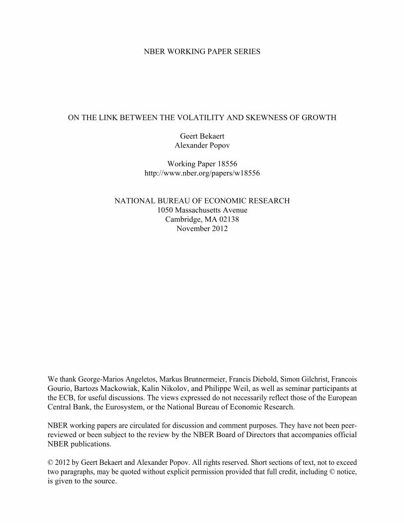
the log of volatility throughout our empirical analysis. Figure 1 plots skewness versus log-

volatility for the 110-country sample and a strong positive relationship is readily apparent.

Table 1, column (1) reports the cross-sectional relationship between the skewness and the

natural logarithm of the standard deviation of GDP growth, calculated over the 1960-2009

period, for the 110 countries in the sample. The estimate of the coefficient in this bivariate

regression is 1.022% and it is significant at the 1% statistical level. The R-squared of the

regression implies that variation in log volatility explains a quarter of the variation in skewness

in the cross-section.

We next wish to establish whether this result is driven by a particular set of countries, or by

a particular time period. Columns (2) and (3) examine whether the relationship is a “rich or poor

country story.” Interestingly, we find that the relationship holds strongly and in a statistically

significant manner in both the lowest and the highest quartile of countries in terms of initial GDP

per capita. Nevertheless, the OLS estimate is almost twice larger for the poorest quartile of

countries relative to the richest quartile of countries, and the R-squared of the regression is 0.42

relative to 0.17. The combined evidence suggests that the positive association between volatility

6

and skewness is stronger for developing countries, but it is not a feature exclusive to developing

countries.

We next split the sample along the growth dimension. We run the main regression on the

countries in the bottom quartile (column (4)) and in the top quartile (column (5)) of the

distribution of average growth over the 1960-2009 period. We thus juxtapose the 28 slowest

growing countries (with an average growth rate of 0.4% over the 50-year period) with the 28

fastest growing countries (with an average growth rate of 4.2%). Strikingly, in both cases the

coefficient of the OLS regression has almost the exact same magnitude. The combined evidence

in columns (2)-(5) thus suggests that our main result is not fully explained by the fact that growth

rates are positively skewed in poor countries, generating a “high growth rate-high volatility”

pattern. Higher volatility is associated with higher skewness at all stages of development and at

all levels of growth.

In columns (6) and (7), we split the sample period in two and re-estimate the cross-

sectional relationship between the skewness and volatility of GDP growth over 1960-1984 and

1985-2009, respectively. The cut-off year corresponds to the beginning of the Great Moderation

(Stock and Watson, 2002), although the second period includes the 2008-09 global financial

crisis. The evidence suggests that the positive association between volatility and skewness is

independent of the period over which the two are measured. However, the relationship is

economically stronger in the post-1984 period, suggesting that GDP growth is more negatively

skewed in a low-volatility environment.

Our results are reminiscent of but different from Ramey and Ramey (1995) who established

that there was a negative trade-off between output growth and volatility. Interestingly, given the

usual utility functions economic agents are endowed with, their stylized fact strongly suggests

high volatility is invariably welfare reducing. Our results, in contrast, suggest that, holding

average growth constant, there may be a true choice between high volatility-high skewness

outcomes and low volatility-low skewness outcomes.

In Table 2, we subject our main stylized fact to a number of data robustness check. First,

we account for the fact that the annual data we are using may not capture properly business cycle

dynamics. In particular, the bust phase may be sharper in annual data. This may systematically

7

bias the results in favour of finding a positive correlation between volatility and skewness if the

busts are sharper in low-volatility countries. We download data on 33 OECD countries from the

STAN Dataset for Industrial Analysis, and re-run our main specification. Column (1) indicates

that the relationship we have uncovered is not due to using less granular data.5

Next, we account for the fact that different updates of the Penn World Table can contain

different real GDP growth series for the same country, despite being derived from similar

underlying data and using almost identical methodologies.6 In some cases, there can be large

differences. For example, according to the 7.0 update that we are using throughout the paper,

Guinea-Bissau recorded a GDP growth rate of 86% in 2005, but according to the 7.1 update the

country grew by 2% in 2005. While such differences do not appear to be systematic, we repeat

the main exercise with data from PWT 7.1. Column (2) indicates that our main result is robust to

this alternative update of PWT. The same is true in column (3) where we calculate volatility and

skewness of GDP growth using PWT 7.0, but we use only 50% of the countries for which the

measure of skewness deviates the least from one version of the Penn Tables to the other.

Finally, the positive association between the volatility and skewness of GDP growth

continues to be statistically and economically significant when we use entirely different data

sources on GDP growth, such as the World Development Indicators (column (4)) and the

International Financial Statistics of the IMF (column (5)).

III. Volatility and Skewness: Fixed Effects Panel Estimates

We now exploit the panel nature of our cross-country dataset. To that end, we calculate

volatility and skewness over reasonably long non-overlapping periods. This allows us to control

for observable time-varying country-specific effects in a model that includes both time- and

country-fixed effects. Specifically, we introduce the following econometric framework:

5 Our results are therefore difficult to reconcile with the reported results in Ordonez (2013). His suggestion that high income countries have more positively skewed output growth than poorer countries is not consistent with either quarterly or annual data. 6 Johnson, Larson, Papageorgiou, and Subramanian (2009) document how the variability of the GDP growth data in different versions of PWT matters for the cross-country growth literature.

8

1 1 ( . .)it it it i t itSkew Ln St dev X

where for each variable we compute its average value over each 5-year period for each country i,

yielding a panel of 1110 observations. itX is a set of time-varying country-specific control

variables to be specified below; i is a matrix of country fixed effects; and t is a matrix of time

fixed effects.

In Table 3, we start with the simplest possible panel regression in which the log standard

deviation of growth is the only regressor and there are country (column (1)) and both country and

time (column (2)) fixed effects. In addition to that, we control for 1-period lagged skewness

(column (3)). Volatility now exerts a negative effect on skewness and this effect is significant at

the 10% level. We confirm this with quarterly data in column (4), for a smaller sub-sample of

(mostly OECD) countries. Here, we have once again calculated the standard deviation and the

skewness of growth over 5-year periods, which in this case yields 20 observations per period.

In columns (5) and (6), analogous to the cross-sectional regression, we split the sample

based on initial GDP per capita. We find that the negative effect is entirely driven by the richer

countries, confirming the result from column (4). This raises the question, at what particular

level of development the negative skewness-volatility relationship becomes apparent. Column

(7) reports the results of a regression where we include the natural logarithm of beginning-of-

period GDP per capita, by itself and interacted with volatility. The coefficient on volatility itself

is now significantly positive but the interaction effect is statistically significantly negative. We

find that the coefficient on volatility turns negative at a per capita GDP level of $1231 (in 2005

dollars), which is at the 28th percentile of the GDP per capita distribution. Rich countries,

controlling for volatility, have significantly lower skewness than poor countries.7

III.A. Recessions and crises

7 This evidence is inconsistent with the predictions laid out in a recent paper by Ordonez (2013). He uses a learning model with endogenous flow of information to argue that financial frictions delay the economy’s recovery after the bust phase. Using quarterly data on (at most) 52 countries, he shows that the skewness of output growth is more negative in less developed economies, a pattern opposite to what we observe in annual data on 110 countries.

9

This evidence has important implications for the calibration of various business cycle

models, especially in emerging markets. Kydland and Zarazaga (2002) and Aguiar and Gopinath

(2007), among others, have suggested that a Real Business Cycle (RBC) model driven by

permanent shocks to productivity can replicate satisfactorily business cycles in developing

countries, in particular the behaviour of output and consumption volatility. Our evidence

suggests that in modelling business cycles in emerging markets, it is important to provide

mechanisms matching higher moments too. In particular, a calibration of RBC models in

emerging markets should be simultaneously mindful of the positive relation between volatility

and skewness over the long-run and of the lack of a negative short-run relation between the

second and third moment of output growth, which is nonetheless prevalent in developed

economies.

What can explain such a “development dependent” relationship between skewness and

volatility? We examine a number of potential channels in Table 4 and discuss them in turn. The

first possibility is simply the asymmetric business cycle variation discussed before when growth

slowdowns or negative growth coincide with high volatility. Aguiar and Gopinath (2007) argue

that in emerging markets trend growth dominates cyclical growth which could explain the lack of

a strong negative relationship for less developed countries. However, Garcia-Cicco, Pancrazi,

and Uribe (2010) now dispute the conclusions in Aguiar and Gopinath (2007) by showing that an

RBC model driven by permanent and transitory productivity shocks captures poorly business

cycle dynamics in two emerging markets, Argentina and Mexico, over 1900-2005. An even

simpler explanation is that crises cause both volatility to increase and skewness to decrease

simultaneously. However, it would be somewhat surprising that developed countries experience

more and more severe crises than do emerging markets. To examine these two hypotheses, we

must measure “crises” and “recessions.” To define a recession, we set a dummy variable equal to

1 if the country experiences negative annual growth at any point during each 5-year period, and

include it in the regression alongside its interaction with the log of the standard deviation of

growth over each 5-year cycle (column (1)). The coefficient on volatility duly turns positive,

whereas the coefficients on the recession dummy and on its interaction with volatility are

10

negative and statistically significant. Hence, the negative association between volatility and

skewness in the full sample is indeed potentially driven by business cycle mechanisms.

III.B. Banking crises and financial development

Next, we use data from Laeven and Valencia (2010) to define a dummy equal to 1 if the

economy is experiencing a systemic banking crisis at any point during each 5-year period, and

include it in the regression together with its interaction with volatility (column (2)). The

coefficients on the variable and on the interaction are negative but (marginally) insignificant,

implying that banking crises do not do fully explain the association between volatility and

skewness in the full sample.

Next, we test for the effect of financial development on the trade-off between volatility and

skewness. In the Kiyotaki and Moore (1997) model of financial frictions, borrowing capacity is a

function of the firm’s net worth and of the state of financial development. Because net worth

fluctuates over the business cycle, real shocks are amplified when the collateral constraint binds,

and whether it does depends on the state of financial intermediation. This model yields three

distinct regimes. For very low levels of financial intermediation, the economy is in autarky as no

borrowing takes place. Because of the absence of leverage, there is no amplification of shocks

and as a result, the growth process is symmetric and characterized by low volatility. Away from

autarky, financial development exerts a non-linear effect on volatility and on skewness. As

financial markets develop initially, economic agents start accumulating leverage. In this case, the

collateral constraint is frequently binding, leading to an amplification of net worth fluctuations

which is manifested in higher output volatility. The more developed the financial system is, the

less frequently the collateral constraint binds. Collateral amplification takes place only when the

negative shocks are sufficiently large, and so the economy is characterized by low volatility and

by negative skewness. This model has a hard time explaining our cross-sectional evidence where

output growth in the highest-volatility countries is very positively skewed. However, as long as

no country in the sample is perfectly financially developed (i.e., the capacity constraint still binds

on the downside), the collateral amplification mechanism can explain the negative temporal

11

correlation between volatility and skewness in the richest countries. We test this story by

including the ratio of private credit to GDP from Beck et al. (2010), on its own and in interaction

with volatility. Column (3) confirms that more financially developed economies have more

negatively skewed business cycles.8 The relationship between volatility and skewness becomes

negative beyond a Private credit / GDP threshold of 0.14 (the 27th percentile of the sample

distribution), suggesting that the negative association between volatility and skewness

documented in Table 2 is driven by business cycle dynamics in relatively financially developed

countries.

III.C. Trade

Next, we investigate the effect of trade openness. Economies more open to trade are in

theory more volatile because they are exposed to terms-of-trade risk (e.g., Rodrik, 1998; Epifani

and Gancia, 2009). We include in the regression a dummy variable equal to 1 if the country is

open to trade at the beginning of each 5-period period, and also an interaction of that variable

with 5-year volatility. Data on trade openness come from Wacziarg and Welch (2008). Column

(4) confirms that trade openness does contribute significantly to the negative skewness of GDP

growth. However, the coefficient on the interaction is (marginally) insignificant, suggesting that

openness to trade is not a crucial determinant of the development-dependent temporal negative

relationship between volatility and skewness.

In column (5), we test for terms-of-trade risk by including the standard deviation of the first

(log) difference of the terms of trade over each respective 5-year period as an independent

variable. We find that terms of trade shocks do not contribute to the positive skewness of growth

rates.

III.D. Government

8 We are therefore puzzled by the claims in Ordonez (2013) which appear contrary to our empirical evidence.

12

We also explore the role of the government sector. Higher government spending can be

associated with a smoother business-cycle because transitory fluctuations are reduced through

automatic stabilisers or discretionary changes in fiscal policy (e.g., Gali, 1994; Fatas and Mihov,

2006). By making recessions milder, government spending may therefore increase the skewness

of growth. Column (6) suggests that government spending increases the skewness of output

growth (albeit insignificantly so), suggesting a more stable business cycle with less pronounced

busts in countries with high government spending. The coefficient on volatility is significantly

negative but the interaction coefficient with government spending is positive and significant,

suggesting that for countries with low government spending, there is a negative trade-off

between volatility and skewness. The interaction effect implies that the association between

volatility and skewness becomes positive beyond a government spending / GDP threshold of

0.18 (the 88th percentile of the distribution). Because government spending excludes social

security, it turns out that the countries exceeding this threshold are actually mostly developing

countries, not the developed countries with mechanisms in place to mitigate the amplitude of the

business cycle. It is therefore also possible that government spending is simply a reverse

indicator of development, just as private credit to GDP and trade openness may also indirectly

rank countries on development status.

III.E. Growth spurts

We now examine the growth spurt mechanism. Various theories provide endogenous

mechanisms for countries to take off and experience growth acceleration after a long period of

underdevelopment characterized by low growth. Some of these theories treat population growth

as fixed (Goodfriend and McDermott, 1995), others propose an explicit mechanism which

considers how population growth and technological growth affect each other (Galor and Weil,

2000; Galor and Moav, 2002). In some models, the economy needs a “lucky draw” to start on an

upward path (Acemoglu and Zilibotti, 1997), and in others, co-ordination is required to achieve

industrialization because no individual sector can break even by industrializing alone (Murphy,

Shleifer, and Vishny, 1989). However, what all these growth theories have in common is a

13

technology-driven transition from a pre-Industrial Revolution equilibrium, characterized by low

GDP growth, to a post-Industrial Revolution equilibrium, characterized by high GDP growth.

These theories have direct implications for our tests: if such growth spurts are large enough (and

thus create volatility), they could induce a large positive temporal correlation between volatility

and skewness. If a sufficient number of countries undergo such episodes, this may account for

the fact that the negative temporal correlation between volatility and skewness that is prevalent

in richer countries is much weaker in the full sample.

To test this prediction, in column (7) we include a variable capturing whether a country is

experiencing a growth spurt during a particular 5-year period. We define a growth spurt using a

dummy variable equal to 1 if the average growth rate over the 5-year period is more than two

standard deviations higher than the sample average, with this average and standard deviation

measured across all countries and time periods. To make sure that we exclude growth spurts

which are due to an outlier in the data potentially reflecting a data error (like Guinea-Bissau’s

86% growth in 2005 according to PWT 7.0), we also require that during this 5-year period, the

country records during at least two years a growth rate which is at least twice higher than the

sample average. We also include the interaction of this variable with volatility. The evidence

confirms the intuition: while volatility and skewness are negatively temporally correlated in the

full sample, the coefficient on the interaction term implies that they become positively correlated

during periods in which the economy is experiencing a growth spurt. Growth spurts themselves

contribute significantly to the positive skewness.

Finally, in column (8) we run a horse race where we include all variables9, as well as their

interactions with volatility, simultaneously in the regression. Tellingly, the only effects that

remain significant are those of recessions, private credit / GDP, and growth spurts. This suggests

that business cycle mechanisms in rich countries and growth spurts in developing countries go a

long way in explaining the development-dependent temporal association between volatility and

skewness.10

9 We exclude the terms-of-trade variable which has too many missing observations. 10 In an unreported regression, we also include GDP per capita and its interaction with volatility in the horse race. Both coefficients are insignificant, implying that the development channels we test in Table 4 explain the development-dependent relationship between volatility and skewness.

14

What is the nature of the growth spurts in our dataset? In traditional models of early

growth, take-off is due to the process of industrialization, i.e., the transition from an economy

based on agriculture to one with a diversified fast-growing manufacturing base. These models

are designed to capture the experience of what are now industrialized countries during the 18th

and 19th century (Galor and Weil, 2000), but they also aim to capture post-WWII developments

which are subsumed in our data period, such as the Big Push in Korea during the 1960s and

1970s (Murphy, Shleifer, and Vishny, 1989). Table 5 lists the growth spurt episodes in our data,

alongside the reason for the rapid growth. From 23 such episodes, 7 can indeed be classified as

Industrial Revolution-type growth spurts: Hong-Kong in 1960-1964, Japan in 1960-1964, Cyprus

in 1965-1969, Malaysia in 1970-1974, Romania in 1975-1979, Singapore in 1970-1974, and

China in 2005-2009. However, the majority of the remaining episodes (13) are related to the

discovery and exploitation of natural resources (mostly oil) and/or a sudden increase in global

demand for such resources or for agricultural products. Three are related to economic

stabilisation and/or liberalization in the wake of political independence or a war.

One subtle distinction that we have not made so far is between growth spurts and “growth

miracles”. While the former are periods of fast growth that may nevertheless be short-lived, the

latter are usually understood as sustained periods of economic growth and convergence in per

capita income. To verify the effect of such growth miracles, we also run a regression

(unreported) including growth miracles in the definition of growth spurts. We define “growth

miracles” as country-specific episodes of at least three consecutive five-year periods with annual

growth higher than 0.05 (the 75th percentile of growth rates in the full sample), and assign a

value of 1 to such episodes. Using this criterion, we add Korea and Taiwan to the sample of

growth spurt countries, resulting in the inclusion of all four “Asian tigers”. The resulting sample

of 21 countries also subsumes the sub-sample of countries which experienced a convergence in

per capita income over the sample period: Botswana and Equatorial Guinea (which moved from

the bottom quartile to the third quartile of per capita GDP) and Korea and Taiwan (which moved

from the bottom quartile to the third quartile of per capita GDP). The main result is robust to this

alternative definition of growth spurt episodes.

15

IV. The Volatility Paradox: Does Low Volatility Breed Negative Skewness?

We are still left with a puzzle. In the cross-section, there is a strong positive association

between the volatility and skewness of growth. In panel data, the relationship is overall negative,

but becomes positive for less developed countries. We documented that asymmetric business

cycles explain the negative coefficient for developed countries. We also showed that growth

spurts in developing countries can explain a temporal positive correlation between volatility and

skewness. How can such patterns lead to the strong positive cross-sectional relationship

documented in Table 1 for all stages of development? Growth spurts explain the positive

relationship in the bottom quartile of countries in terms of GDP per capita. However, the

evidence we have presented does not reconcile the strong negative temporal association between

volatility and skewness with the strong positive long-term association between the two in the top

echelon of countries in terms of per capita wealth (Table 1, column (3)), especially after 1984

(the year of the commonly accepted start of the Great Moderation). If anything, rich countries

with deeper recessions should have a higher long-term volatility than rich countries with less

deep recessions, inducing a negative cross-sectional variation between long-run volatility and

long-run skewness. At the same time, however, some rich countries have experienced large

macroeconomic contractions because they had low volatility for too long, which led to over-

leveraging and a sharp financial crisis. This is a temporal but not a contemporaneous relation

between low volatility and negative skewness that can help explain the positive long-run

association between the two in the cross-section. By populating the high and low quadrant of the

cross-sectional distribution of volatility correctly, the cross-sectional relationship becomes

strongly positive. We explore this “story” now in more detail.

A narrative going back to Minsky (1986) suggests that good (high-growth, low-volatility)

times give rise to speculative investor euphoria, and soon thereafter debts exceed what borrowers

can pay off from their incoming revenues, which in turn leads to a financial crisis. As a result of

the collapse of the speculative borrowing bubble, investors – and especially banks – reduce

credit availability, even to companies that can afford to borrow, and the economy subsequently

contracts. This narrative suggests that past volatility and future skewness can correlate positively.

16

Building on similar models by Bernanke and Gertler (1989), Bernanke, Gertler, and Gilchrist

(1996), and Kiyotaki and Moore (1997), Brunnermeier and Sannikov (2013) formalize this story

through a mechanism in which agents react to an exogenous decline in macroeconomic risk by

accumulating higher leverage. As a result, a low exogenous risk environment is conducive to a

greater build-up of systemic risk. In this setting, instability is higher when aggregate risk is low,

implying that a period of low volatility should be followed by a sharp crisis (a period of negative

skewness), especially in economies whose financial markets are developed enough as to enable a

build-up of leverage beyond the critical threshold. If reaching particular low levels of volatility

was associated with an increased propensity for large, abrupt, and rare macroeconomic

contractions in the future, this could explain a positive link between volatility and skewness at

high levels of financial development.

In Table 6, we test these implications of the Brunnermeier-Sannikov model in a number of

ways. First, we regress the skewness of GDP growth onto the lagged standard deviation of GDP

growth and on lagged private credit / GDP, plus the interaction between the two. In the full

sample, not surprisingly, we do not find any statistically significant coefficient. The

Brunnermeier–Sannikov model is only relevant for economies that have sufficiently developed

financial sectors. In the second column, we focus on the top tertile of the sample in terms of

average private credit / GDP over the 1960-2009 period. Now all three coefficients are

significant at a minimum at the 10% level. At relatively low levels of financial development, low

past volatility is still negatively associated with future skewness; however, at private credit /

GDP levels of more than 1.05, the relationship turns positive. While the threshold may seem

somewhat high, there are 23 countries in the sample that experience private credit / GDP levels

beyond that threshold during at least one 5-year period. These regressions also include country

and time fixed effects and the controls used in Table 4. These tests thus provide strong evidence

that periods of low volatility may be causally linked to future periods of crises (negative

skewness), especially for countries in later stages of financial development.

In the next two columns, we test an alternative specification. In particular, we define a “low

volatility duration” regime, in the following way. We create a variable equal to 1 if the country is

experiencing a 5-year GDP growth volatility of less than 0.013 (the bottom 10th percentile of the

17

overall sample distribution of 5-year volatility). If volatility was also less than 0.013 in the

previous period, we give the variable a value of 1.75 (1 + 0.75), and a value of 2.31 (1.75 + .752)

if two periods ago volatility was also less than 0.013, and so on. As a consequence, we over-

weight longer duration low volatility regimes, decaying the effect by 0.75 per 5 year block.11

Then we interact this variable with private credit / GDP and replicate the regression reported in

the first two columns where instead of volatility we employ this new “low volatility duration”

indicator. Columns (3) and (4) of Table 6 indicate that while the association between volatility

and skewness does not depend on financial development in the full sample, it does, and

significantly so, in the set of countries in the top tertile of the sample in terms of average private

credit / GDP over 1960-2009. The magnitude of the coefficients implies that while prolonged

periods of low volatility are positively associated with GDP growth skewness, the relation turns

negative at private credit / GDP levels of more than 0.98. We note that 26 countries in our

sample experienced at least one 5-year period during which private credit / GDP was beyond that

threshold. In 12 of these, the combination of a period of low volatility and over-the-threshold

levels of domestic credit was followed by a systemic banking crisis, as defined by Laeven and

Valencia (2010).12

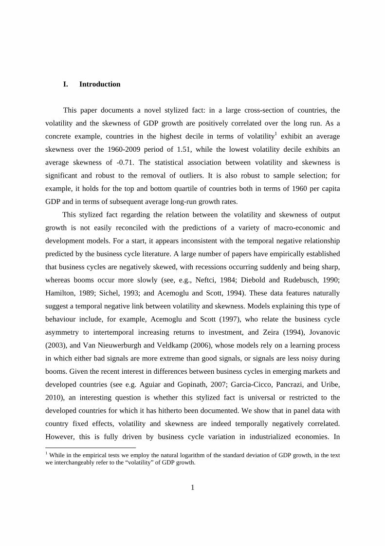
Figures 2 and 3 illustrate the two main mechanisms which are at play in the cross-section in

the long run. The evolution of GDP growth in Equatorial Guinea (Figure 2) is marked by the

discovery of large oil fields in 1996. As a result of their subsequent exploration, Equatorial

Guinea experienced a rapid growth spurt; for example, its GDP tripled between 1996 and 1998.

This development is mapped into the highest growth volatility over 1960-2009 in our sample,

0.242, as well as the third highest skewness, 2.676, although prior to 1996 the country’s

economy was characterized by a symmetric and relatively steady (low) growth process.

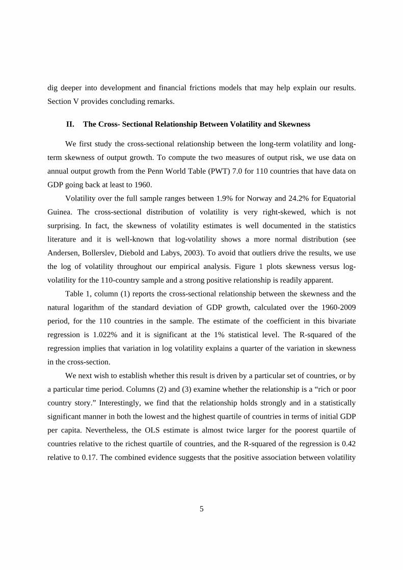
At the opposite end of the development cycle is the UK (Figure 3). Characterized by a low-

volatility growth all the way up to the recent crisis, its economy experienced a very deep

contraction in 2009 following the banking crisis of 2007-08. The resulting skewness of -1.176 is

11 The results are robust to alternative weighting schemes. 12 These countries are: Austria (2008-), Denmark (2008-), France (1998), Japan (1997-1998 and 2008-) Malaysia (1997-1999), Netherlands (2008-), Portugal (2008-), Spain (2008-), Sweden (1991-1995 and 2008-), Switzerland (2008-), the United Kingdom (2008-), and the United States (2008-).

18

one of the lowest in the cross-section, despite the fact that UK’s growth volatility over 1960-

2009 is the fourth lowest at 0.020.

V. Conclusion

In a sample of 110 countries during the 1960-2009 period, volatility and skewness are

temporally negatively correlated in panel data with country fixed effects, but positively

correlated in the cross-section. While the former fact is consistent with rich countries’ business

cycles where volatility is high during recessions, the latter fact is novel and somewhat puzzling.

For example, in a number of business cycle theories the skewness of GDP growth is hardwired in

the business cycle due to learning asymmetries and so is orthogonal to the standard deviation of

the distribution of real shocks (e.g., Van Nieuwerburgh and Veldkamp, 2006). Theories of early

development and industrialization (e.g., Acemoglu and Zilibotti, 1997) do not fully explain the

prevalence of low-volatility low-skewness countries in the sample, and financial accelerator-type

theories (e.g., Bernanke and Gertler, 1989; Kiyotaki and Moore, 1997) have no mechanism for

generating a high-volatility positive-skewness growth profile.

We argue that there are two main forces at play in the cross-section. First, a number of

developing countries experience abrupt economic expansions, which can be short-lived (growth

spurts) or sustained (“growth miracles”). While some are related to industrialization, most are the

outcome of the discovery and exploitation of natural resources, and others are due to

macroeconomic stabilisation following political conflict. Second, a number of low-volatility

countries experience systemic financial crises followed by large contractions, consistent with the

mechanism in Minsky (1986) and Brunnermeier and Sannikov (2013). While such countries

experience the highest volatility during the contractions (explaining the temporally negative

association between volatility and skewness), the relative magnitude of the contraction is

inversely related to the preceding long-term volatility. These two phenomena jointly explain the

co-existence of high-volatility positive-skewness and of low-volatility negative-skewness

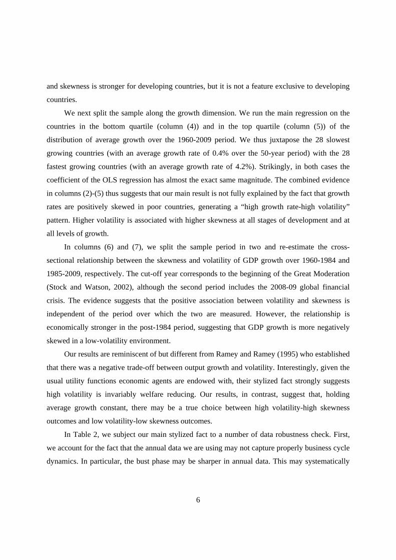
countries in the cross-section. They are illustrated in Figure 4 where the growth spurt countries

occupy the upper right quadrant of the data points, and the financially developed countries that

experience high levels of aggregate private leverage occupy the lower left quadrant.

19

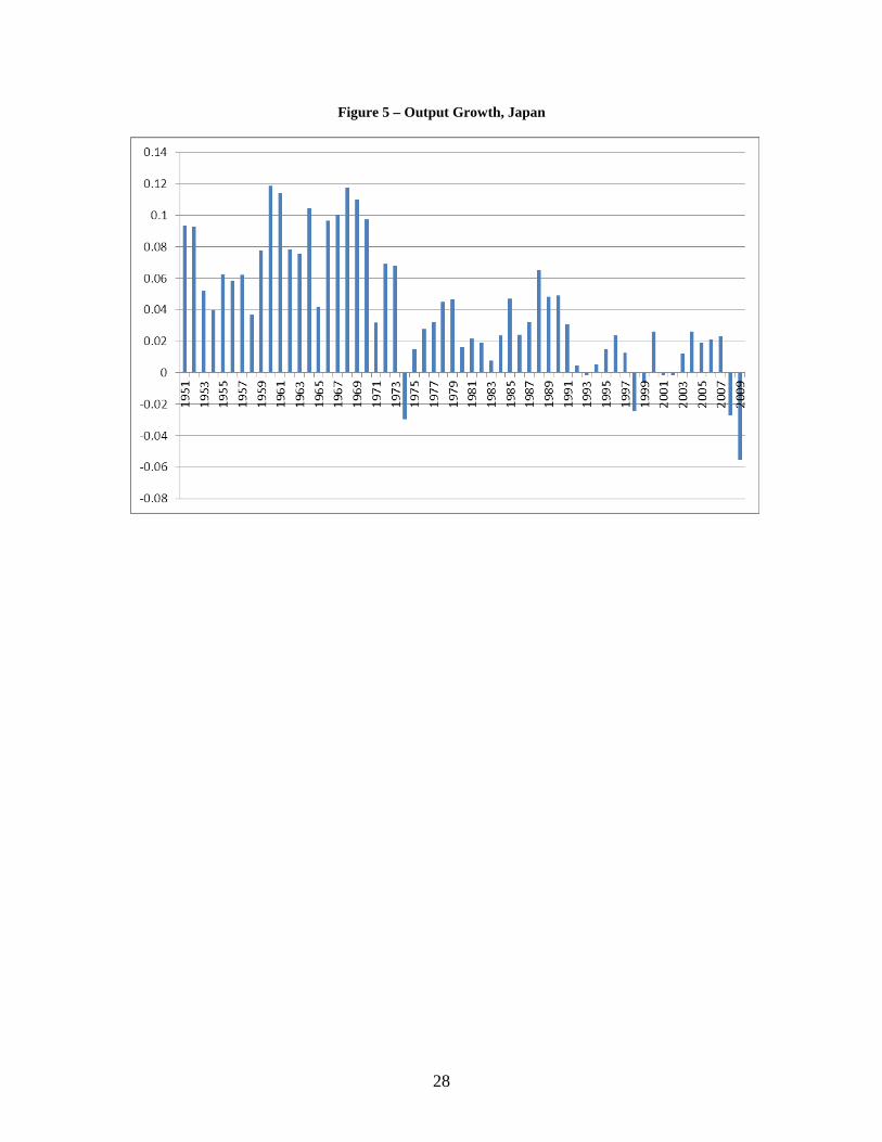
While we invoke two separate mechanisms to explain the positive correlation between

volatility and skewness in the cross-section, our data contains examples of a single country

subject to both mechanisms in the long run. Figure 5 presents the evolution of GDP growth in

Japan between 1950 and 2009. The first period, between 1951 and 1973, is characterized by high

albeit volatile growth, following rapid industrialization in the wake of WWII. The second period,

between 1975 and 2009, is a period of slower economic growth and lower volatility, especially

after 1991. This same period contains two systemic financial crises, the one following the dual

stock market and real estate boom of the 1980s and the global financial crisis of 2008-09. Thus,

Japan illustrates how a country can in a fairly short time period go from an emerging

industrializing economy characterized by high, volatile, positively-skewed growth process to a

low-growth low-volatility industrialized country with a highly developed financial sector13 that

can accumulate excessive debt and cause a systemic crisis. Recent unified growth models

provide an endogenous mechanism for the transition from pre- to post-industrialization based on

the accumulation of knowledge (Galor and Weil, 2000; Hansen and Prescott, 2002). However,

we are not aware of growth models that also capture the “late” stage of development

characterized by low volatility and occasional severe recessions led by financial crises. Our

evidence calls for theoretical endeavors in this direction.

13 After Iceland in 2006 and Cyprus in 2009, Japan in 1998 had the highest ratio of private credit to GDP in our sample, at 2.31.

20

References

Acemoglu, D., and A. Scott, 1994. Asymmetries in the cyclical behavior of UK labor

markets. Economic Journal 104, 1302-1323.

Acemoglu, D., and A. Scott, 1997. Asymmetric business cycles: Theory and time-series

evidence. Journal of Monetary Economics 40, 501-533.

Acemoglu, D., and F. Zilibotti, 1997. Was Prometheus unbound by chance? Risk,

diversification, and growth. Journal of Political Economy 105, 709-751.

Acemoglu, D., Johnson, S., Robinson, J., and Y. Thaicharoen, 2003. Institutional causes,

macroeconomic symptoms: Volatility, crises and growth. Journal of Monetary Economics 50,

49-123.

Aguiar, M., and G. Gopinath, 2007. Emerging market business cycles: The cycle is the

trend. Journal of Political Economy 115, 69-102.

Andersen, T., Bollerslev, T., Diebold, F.X., and P. Labys, 2003. Modelling and forecasting

realized volatility. Econometrica 71, 576-625.

Beck, T., Demirgüç-Kunt, A., and R. Levine, 2010. A new database on financial

development and structure. World Bank Economic Review 14, 597-605.

Bernanke, B., and M. Gertler, 1989. Agency costs, net worth, and business fluctuations.

American Economic Review 79, 14-31.

Bernanke, B., Gertler, M., and S. Gilchrist, 1996. The financial accelerator and the flight to

quality. Review of Economics and Statistics 78, 1-15.

Bloom, D., David, C., and S. Jaypee, 2003. Geography and poverty traps. Journal of

Economic Growth 8, 355-378.

Brunnermeier, M., and Y. Sannikov, 2013. A macroeconomic model with a financial

sector. American Economic Review, forthcoming.

Comin, D., and M. Gertler, 2006. Medium-term business cycles. American Economic

Review 96, 523-550.

Dewachter, H., and R. Wouters, 2012. Endogenous risk in a DSGE model with capital-

constrained financial intermediaries. Mimeo.

21

Diebold, F., and G. Rudebusch, 1990. A non-parametric investigation of duration

dependence in the American business cycle. Journal of Political Economy 98, 596-616.

Epifani, P., and G. Gancia, 2009. Openness, government size, and terms of trade. Review of

Economic Studies 76, 629-668.

Fatah, A., and I. Mihov, 2006. The macroeconomic effects of fiscal rules in the US states.

Journal of Public Economics 90, 101-117.

Galor, O., and D. Weil, 2000. Population, technology, and growth: From Malthusian

stagnation to the demographic transition and beyond. American Economic Review 90, 806-828.

Galor, O., and O. Moav, 2002. Natural selection and the origin of economic growth.

Quarterly Journal of Economics 117, 1133-1191.

Garcia-Cicco, J., Pancrazi, R., and M. Uribe, 2010. Real business cycles in emerging

countries? American Economic Review 100, 2510–2531.

Gali, J., 1994. Government size and macroeconomic stability. European Economic Review

38, 117-132.

Goodfriend, M., and J. McDermott, 1995. Early development. American Economic Review

85, 116-133.

Hamilton, J., 1989. A new approach to the economic analysis of non-stationary time series

and the business cycle. Econometrica 57, 357-384.

Hansen, G., and E. Prescott, 2002. Malthus to Solow. American Economic Review 92,

1205-1217.

He, Z., and A. Krishnamurty, 2012. A macroeconomic framework for quantifying systemic

risk. Mimeo.

Johnson, S., Larson, W., Papageorgiou, C., and A. Subramanian, 2009. Is newer better?

Penn World Table revisions and their impact on growth estimates. NBER Working Paper 15455.

Jovanovic, B., 2006. Asymmetric cycles. Review of Economic Studies 73, 145-162.

Kiyotaki, N., and J. Moore, 1997. Credit cycles. Journal of Political Economy 105, 211-

248.

Kydland, F., and C. Zarazaga, 2002. Argentina’s lost decade. Review of Economic

Dynamics 5, 152-165.

22

Laeven, L., and F. Valencia, 2010. Resolution of banking crises: The good, the bad, and the

ugly. IMF working paper 10/146.

Mendoza, E., 2010. Sudden stops, financial crises, and leverage. American Economic

Review 100, 1941-1966.

Minsky, H, 1986. Stabilizing an Unstable Economy. New Haven: Yale University Press.

Murphy, K., Shleifer, A., and R. Vishny, 1989. Industrialization and the Big Push. Journal

of Political Economy 97, 1003-1026.

Neftci, S., 1984. Are economic time series asymmetric over the business cycle? Journal of

Political Economy 92, 307-328.

Ordonez, G., 2013. The asymmetric effects of financial frictions. Journal of Political

Economy, forthcoming.

Owen, A., Videras, J., and L. Davis, 2009. Do all countries follow the same growth

process? Journal of Economic Growth 14, 265-286.

Ramey, G., and V. Ramey, 1995. Cross-country evidence on the link between volatility and

growth. American Economic Review 85, 1138-1151.

Ranciere, R., A. Tornell, and F. Westermann, 2008. Systemic Crises and Growth.

Quarterly Journal of Economics, 359-406.

Reinhart, C., and K. Rogoff, 2011. From financial crash to debt crisis. American Economic

Review 101, 1676-1706.

Rodrik, D., 1998. Why do more open economies have bigger governments? Journal of

Political Economy 106, 997-1032.

Sachs, J., and A. Warner, 1995. Economic reform and the process of global integration.

Brookings Papers on Economic Activity 1, 1-118.

Sichel, D., 1993. Business cycle asymmetry: a deeper look. Economic Inquiry 31, 224-236.

Stock, J., and M. Watson, 2002. Has the business cycle changed and why? NBER Chapters,

in: NBER Macroeconomics Annual 17, 159-230.

Van Nieuwerburgh, S., and L. Veldkamp, 2006. Learning asymmetries in real business

cycles. Journal of Monetary Economics 53, 753-772.

23

Wacziarg, R., and K. Welch, 2008. Trade liberalization and growth: New evidence. World

Bank Economic Review 22, 187-231.

Welch, I., 1992. Sequential sales, learning, and cascades. Journal of Finance 47, 695-732

Zeira, J., 1994. Informational cycles. Review of Economic Studies 61, 31-44.

24

Figure 1 - Skewness of Output Growth against Log Standard Deviation of Output Growth, 110 Countries, 1960-2009

-20

24

Ske

wne

ss o

f out

put g

row

th, 1

960-

2009

-4 -3.5 -3 -2.5 -2 -1.5Log standard deviation of output growth, 1960-2009

25

Figure 2 - Output Growth, Equatorial Guinea

Growth = 0.098; St. dev. = 0.242; Skewness = 2.676

-0.4

-0.2

0

0.2

0.4

0.6

0.8

1

1.2

1.4

1961

1964

1967

1970

1973

1976

1979

1982

1985

1988

1991

1994

1997

2000

2003

2006

2009

Equatorial Guinea

01

23

-.5 0 .5 1 1.5Equatorial Guinea

kernel = epanechnikov, bandwidth = 0.0529

Kernel distribution of real GDP growth, 1960-2009

26

Figure 3 - Output Growth, United Kingdom

Growth = 0.008; St. dev. = 0.020; Skewness = -1.176

-0.1

-0.08

-0.06

-0.04

-0.02

0

0.02

0.04

0.06

0.08

0.1

1960

1963

1966

1969

1972

1975

1978

1981

1984

1987

1990

1993

1996

1999

2002

2005

2008

United Kingdom

010

2030

-.1 -.05 0 .05 .1United Kingdom

kernel = epanechnikov, bandwidth = 0.0057

Kernel distribution of real GDP growth, 1960-2009

27

Figure 4 - Low Volatility Bank Crisis Countries and Growth Spurt Countries

-20

24

Ske

wne

ss o

f out

put g

row

th, 1

960-

2009

-4 -3.5 -3 -2.5 -2 -1.5Log standard deviation of output growth, 1960-2009

Low-volatility bank crisis countries Growth spurt countriesMiddle countries Fitted values

28

Figure 5 – Output Growth, Japan

29

Table 1 –The Skewness of GDP Growth and the Natural Logarithm of the Standard Deviation of GDP Growth: Cross-Sectional Results

Full sample 1st quartile, initial

development 4th quartile, initial

development 1st quartile,

growth 4th quartile,

growth

1960-1984

1985-2009 (1) (2) (3) (4) (5) (6) (7)

Log (St. dev. GDP growth) 1.022*** 1.398*** 0.684** 1.075*** 1.104*** 0.366** 1.104*** (0.167) (0.307) (0.266) (0.323) (0.163) (0.142) (0.163) Observations 110 28 28 28 28 110 110 R-squared 0.25 0.42 0.17 0.20 0.30 0.06 0.30

Notes: The skewness and the standard deviation of GDP growth are calculated for all countries in the sample for the 1960-2009 period (column (1)-(5)), for the 1960-1984 period (column (6)), and for the 1985-2009 period (column (7)). Data on GDP growth from the 7.0 update of the Penn World Table are used. Initial development quartiles are determined based on GDP per capita in 1960. Growth quartiles are determined based on average GDP growth over the 1960-2009 period. Standard errors are provided in parentheses. *** indicates a p-value less than 0.01, ** indicates a p-value less than 0.05.

30

Table 2 –The Skewness of GDP Growth and the Natural Logarithm of the Standard Deviation of GDP Growth: Cross-Sectional Results from Alternative Data Sources

STAN quarterly

data

PWT 7.1 data PWT 7.0 and

7.1 data

WDI data

IFS data (1) (2) (3) (4) (5)

Log (St. dev. GDP growth) 0.864** 0.803*** 0.797*** 0.688*** 0.522*** (0.428) (0.178) (0.221) (0.221) (0.148) Observations 33 110 55 89 142 R-squared 0.12 0.16 0.18 0.09 0.08

Notes: The skewness and the standard deviation of GDP growth are calculated for all countries in the sample for the 1960-2009 period. In column (1), quarterly data on GDP growth from the STAN Dataset on Industrial Analysis are used to calculate long-run volatility and skewness. In column (2), data on GDP growth are from the 7.1 update of the Penn World Table. In column (3), data on GDP growth are from the 7.0 update of the Penn World Tables, and the top 50% of the countries in terms of the difference in skewness between the 7.0 and the 7.1 update are dropped. In column (4), data on GDP growth are from the World Bank’s World Development Indicators. In column (5), data on GDP growth are from the IMF’s International Financial Statistics. Standard errors are provided in parentheses. *** indicates a p-value less than 0.01, ** indicates a p-value less than 0.05.

31

Table 3 - The Skewness of GDP Growth and the Natural Logarithm of the Standard Deviation of GDP Growth: Panel Regression Results

Full sample Full sample Full sample Quarterly data

1st quartile 4th quartile Full sample

(1) (2) (3) (4) (5) (6) (7)

Log (St. dev. 5-year GDP growth) -0.059* -0.058* -0.064* -0.276* 0.013 -0.213*** 0.512*** (0.034) (0.034) (0.036) (0.165) (0.063) (0.075) (0.199) 1-period lagged 5-year GDP -0.107*** skewness (0.034) Log (GDP per capita) -0.293*** (0.103) Log (5-year output volatility)× Log (GDP per capita) -0.072*** (0.025) Country dummies Yes Yes Yes Yes Yes Yes Yes Period dummies No Yes Yes Yes Yes Yes Yes Observations 1100 1100 990 169 280 280 280 Countries 110 110 110 33 28 28 28 R-squared 0.01 0.03 0.03 0.33 0.01 0.20 0.06

Notes: The skewness and the standard deviation of GDP growth are calculated for all countries in the sample for five-year non-overlapping periods over 1960-2009. Annual data on GDP growth from the 7.0 update of the Penn World Table are used (columns (1)-(3) and columns (5)-(7)). In column (4), quarterly data on GDP growth from the STAN Dataset on Industrial Analysis are used. GDP per capita refers to the country’s per capita GDP in the beginning of each 5 year period. The regressions include country and period fixed effects. In columns (5) and (6), quartiles are determined based on GDP per capita in 1960. Standard errors are provided in parentheses. *** indicates a p-value less than 0.01, * indicates a p-value less than 0.10.

32

Table 4 - The Skewness of GDP Growth and the Natural Logarithm of the Standard Deviation of GDP Growth: Country Heterogeneity

Recession

(1)

Banking crisis (2)

Private credit / GDP

(3)

Trade liberalization

(4)

Terms of trade (5)

Government spending/GDP

(6)

Growth spurt

(7)

Horse race (8)

Log (St. dev. 5-year GDP growth) 0.138** -0.037 0.049 -0.017 -0.145** -0.159*** -0.092*** 0.147 (0.056) (0.036) (0.048) (0.043) (0.072) (0.061) (0.035) (0.098) Recession -0.837*** -0.843*** (0.241) (0.290) Banking crisis -0.391 -0.225 (0.323) (0.333) Private credit / GDP -1.342*** -0.742** (0.334) (0.356) Trade liberalization -0.396* -0.261 (0.232) (0.263) St. dev. (Terms of trade) 6.021 --------- (3.930) Government spending / GDP 2.389 0.940 (1.456) (1.586) Growth spurt 1.775*** 1.301** (0.504) (0.528) Log (St. dev. 5-year GDP growth)× -0.111* -0.124* Recession (0.064) (0.076) Log (St. dev. 5-year GDP growth)× -0.056 -0.018 Banking crisis (0.096) (0.098) Log (St. dev. 5-year GDP growth)× -0.357*** -0.212** Private credit/GDP (0.089) (0.096) Log (St. dev. 5-year GDP growth)× -0.106 -0.023 Trade liberalization (0.065) (0.072) Log (St. dev. 5-year GDP growth)× 1.946* --------- Log (Terms of trade) (1.138) Log (St. dev. 5-year GDP growth)× 0.907** 0.426 Government spending/ GDP (0.453) (0.499) Log (St. dev. 5-year GDP growth)× 0.481** 0.432** Growth spurt (0.202) (0.212) Country dummies Yes Yes Yes Yes Yes Yes Yes Yes Period dummies Yes Yes Yes Yes Yes Yes Yes Yes

33

Notes: The skewness and the standard deviation of GDP growth are calculated for all countries in the sample for five-year non-overlapping periods over 1960-2009. Data on GDP growth from the 7.0 update of the Penn World Table are used. Recession is an indicator variable equal to 1 if the country experiences at least 1 year of negative GDP growth during each respective five-year period. Banking crisis is an indicator variable equal to 1 if the country experiences a systemic banking crisis as defined by Laeven and Valencia (2010) during each respective five-year period. Private credit / GDP is the average of the ratio of credit to the private sector to GDP during each respective 5-year period. Trade liberalization is an indicator variable equal to 1 if the country has liberalized trade according to the Wacziarg and Welch (2008) classification at the beginning of each respective five-year period. St. dev. (Terms of trade) is the standard deviation of the first (log) difference of the terms of trade over each respective 5-year period. Growth spurt is an indicator variable equal to 1 if the country experiences an average growth rate higher than the sample average by two standard deviations or more during each respective five-year period. The threshold corresponds to an average annual growth of 0.095 over five years. All regressions include country and period fixed effects. Standard errors are provided in parentheses. *** indicates a p-value less than 0.01, ** indicates a p-value less than 0.05, * indicates a p-value less than 0.10.

Observations 1100 1100 977 1100 569 1100 1100 977 R-squared 0.05 0.05 0.06 0.05 0.03 0.05 0.09 0.09

34

Table 5 - Growth Spurt Episodes

Country

Period

Average annual GDP growth

GDP skewness, 1960-2009

Event

Botswana 1970-1974 0.194 0.531 In 1966, newly independent Botswana embarks on a program of economic liberalization under Prime Minister (and later President) Khama.

1985-1989 0.100 0.531 Diamonds are discovered. Diamonds now constitute 62% of Botswana’s exports. Chad 2000-2004 0.112 1.132 Oil production starts in 2003. By 2008, oil revenues constitute 41% of GDP. China 2005-2009 0.097 -1.304 The economy of China growth by more than 11.5% annually between 2005 and 2007, fuelled by strong foreign demand for its exports. Republic of the Congo

1970-1974 0.103 0.332 Rapid increase in oil production and exports. 1980-1984 0.097 0.332 Oil production continues to expand. Per capita GDP more than doubles between 1970

and 1984. Cyprus 1965-1969 0.104 -0.283 Rapid transition from agriculture to manufacturing in the wake of gaining

independence from Great Britain. 1975-1979 0.102 -0.283 The economy recovers after the 1974-1975 war during which per capita GDP declined

by 31% in two years. Equatorial Guinea 1995-1999 0.545 2.676 Discovery and subsequent exploration of large oil reserves. As a result, Equatorial

Guinea has emerged as the third-largest oil producer in Sub-Saharan Africa. 2000-2004 0.266 2.676 Gabon 1970-1974 0.113 0.585 Oil was discovered offshore in the early 1970s. At present, the oil sector accounts for 50% of GDP and 80% of exports. Gambia 2005-2009 0.115 1.780 Strong sustained economic growth driven by tourism and agricultural exports. Hong Kong 1960-1964 0.119 0.505 Hong Kong continues the policy of rapid industrialization embarked upon in the 1950s. Japan 1960-1964 0.098 0.383 Rapid industrialization, continuing a trend since the early 1950s. Malawi 1965-1969 0.136 0.726 Rapid economic growth based on the export of agricultural products. Malaysia 1970-1974 0.099 -0.269 Rapid industrialization from a mining- and agriculture-based economy to a multisector economy Mauritania 1960-1964 0.126 2.613 Iron mines start operating in 1963. Morocco 1960-1964 0.109 0.496 The government embarks on a 5-year plan for the development and modernization of the agricultural sector. Nigeria 1970-1974 0.102 0.369 Rapid expansion of oil production. In 2000, oil and gas exports represent more than 98% of export earnings and 83% of government revenues. Romania 1975-1979 0.096 -0.636 Rapid state-enforced industrialization. Singapore 1970-1974 0.102 -0.969 Following separation from Malaysia in 1965, the government adopts a pro-foreign

investment, export-oriented economic policy combined with investment in strategic government-owned companies.

Trinidad and 2005-2009 0.100 0.216 A global demand-driven boom in the production of oil, petrochemicals, and liquefied Tobago natural gas.

35

Zambia 2000-2004 0.150 2.780 Substantial growth in copper exports due to rising world prices. At present, copper and copper products constitutes 69% of Zambia’s exports.

36

Table 6 - The Skewness of GDP Growth and the Natural Logarithm of the Standard Deviation of GDP Growth: Testing for the “Volatility Paradox”

Full sample Top 33%

private credit

Full sample Top 33%

private credit (1) (2) (3) (4) 1-period lagged log (St. dev. 5-year GDP growth)×1-period 0.058 0.201* lagged private credit / GDP (0.087) (0.123) 1-period lagged log (St. dev. 5-year GDP growth) -0.011 -0.211* (0.049) (0.127) Low volatility duration×1-period lagged 0.049 -0.440** private credit / GDP (0.146) (0.210) Low volatility duration -0.022 0.431** (0.106) (0.192) 1-period lagged private credit / GDP 0.334 0.957* 0.030 0.211 (0.371) (0.508) (0.113) (0.164) Country variables Yes Country dummies Yes Period dummies Yes Observations 901 331 977 331 Countries 108 36 108 36 R-squared 0.08 0.19 0.07 0.18

Notes: The skewness of GDP growth, the standard deviation of GDP growth, and the ratio of private sector to GDP are calculated for all countries in the sample for 10 five-year periods over 1960-2009. Low volatility duration refers to the sum of consecutive periods during which the country experiences volatility of GDP growth lower by two standard deviations or more than the sample average. The current period is given a weight of 1, the previous period a weight of 0.75, the one before a weight of 2.31, etc. (see Section IV for details). Data on GDP growth from the 7.0 update of the Penn World Table are used. The regressions include the rest of the explanatory variables from Table 4, as well as country and period fixed effects. Standard errors are provided in parentheses. ** indicates a p-value less than 0.05, * indicates a p-value less than 0.10.

37

Appendix 1 - Description of Variables

Variable Description Standard deviation of GDP growth Standard deviation of the growth rate of GDP. Calculated over the

1960-2009 in the cross-section regressions, or over non-overlapping 5-year periods in the panel regressions. The underlying data on GDP growth (GRGDPCH) come from the World Penn Tables.

Skewness of GDP growth The skewness of the growth rate of GDP. Calculated over the 1960-2009 in the cross-section regressions, or over non-overlapping 5-year periods in the panel regressions. The underlying data on GDP growth (GRGDPCH) come from the World Penn Tables.

Initial GDP per capita GDP per capita (RGDPCH) in 1960, from the Wold Penn Tables, in PPP converted 2005 constant prices.

GDP per capita Average GDP per capita (RGDPCH) for non-overlapping 5-year periods, from the Wold Penn Tables, in PPP converted 2005 constant prices.

Recession A dummy variable equal to 1 if the country experiences a negative growth in at least one year during each non-overlapping 5-year period. The underlying data on GDP growth (GRGDPCH) come from the World Penn Tables.

Banking crisis A dummy equal to 1 if the country experiences a systemic banking crisis during each non-overlapping 5-year period. The underlying data come from Laeven and Valencia (2010)

Private credit / GDP The value of total credits by financial intermediaries to the private sector in each country, excluding credit by central banks. From Beck et al. (2010).

Trade liberalization Terms of trade

A dummy equal to 0 (that is, a country is judged as “closed”) if any of the following five criteria holds: average tariffs are 40% or more; non-tariff barriers cover 40% or more of trade; the black market exchange rate is at least 20% lower than the official exchange rate; a state monopoly exists on major exports; and the economic system is socialist (see Wacziarg and Welch (2008)’s revision of the original Sachs and Warner (1995) classification of trade openness episodes) The percentage ratio of the export unit value indices to the import unit value indices, measured relative to the base year (2000). From the World Bank Development Indicators

Government spending The share of government consumption of PPP converted GDP per capita at current prices. The underlying data (KG) come from the World Penn Tables.

Growth spurt A dummy equal to 1 if over a non-overlapping 5-year period the country is experiencing a) average growth higher than 0.095 (which corresponds to growth higher than the average growth for the sample by two standard deviations), and b) at least two years of high growth (more than twice the sample average). The underlying data on GDP growth (GRGDPCH) come from the World Penn Tables.

38

Appendix 2 - Summary Statistics

Country St. dev. of

GDP growth Skewness of GDP growth

Initial GDP per capita

GDP per capita Recession Banking crisis

Private credit / GDP

Trade liberalization

Government spending

Growth spurt

Algeria 0.082 -1.533 4078.73 4586.25 0.9 0.1 0.308 0.0 0.12 0 Argentina 0.047 -0.360 6243.57 7957.05 0.9 0.5 0.182 0.3 0.08 0 Australia 0.019 -0.721 13116.90 23875.46 0.4 0.0 0.555 0.9 0.10 0 Austria 0.025 0.514 10632.79 23130.55 0.3 0.1 0.753 1.0 0.10 0 Bangladesh 0.039 -1.227 802.07 839.15 0.7 0.1 0.167 0.2 0.02 0 Barbados 0.053 -0.252 7647.78 17739.93 0.8 0.0 0.511 0.8 0.15 0 Belgium 0.023 -0.616 10240.59 22071.37 0.4 0.1 0.429 1.0 0.11 0 Benin 0.057 0.793 801.33 1001.16 0.8 0.2 0.154 0.4 0.10 0 Bolivia 0.036 -2.291 2713.58 3043.50 0.7 0.2 0.252 0.5 0.08 0 Botswana 0.103 0.531 578.04 4047.99 0.8 0.0 0.140 0.6 0.10 0.2 Brazil 0.042 0.053 2581.05 5664.59 0.5 0.1 0.426 0.3 0.11 0 Burkina Faso 0.058 1.364 589.88 662.76 0.9 0.1 0.106 0.2 0.14 0 Burundi 0.076 1.215 258.73 356.28 1.0 0.2 0.104 0.2 0.18 0 Cameroon 0.056 0.128 1241.29 1688.94 0.9 0.3 0.161 0.3 0.06 0 Canada 0.021 -0.911 12987.91 24286.42 0.4 0.0 0.816 1.0 0.10 0 Cape Verde 0.070 -0.471 1052.97 1613.07 0.5 0.1 0.315 0.3 0.13 0 Central African 0.043 -0.234 1073.57 840.03 1.0 0.2 0.103 0.0 0.19 0 Chad 0.088 1.132 818.61 842.15 1.0 0.3 0.076 0.0 0.51 0.1 Chile 0.055 -1.715 3780.41 5990.72 0.8 0.3 0.455 0.6 0.07 0 China 0.060 -1.304 846.79 1931.41 0.5 0.1 0.859 0.0 0.16 0.1 Colombia 0.035 1.427 2478.32 4244.86 0.8 0.3 0.264 0.4 0.05 0 Comoros 0.048 0.744 757.21 1167.24 0.9 0.0 0.123 0.0 0.32 0 Congo, Dem. Rep. 0.131 1.486 1092.26 709.63 1.0 0.3 0.022 0.0 0.06 0 Congo, Rep. 0.077 0.332 791.10 1773.67 0.8 0.0 0.144 0.0 0.11 0.2 Costa Rica 0.033 -1.326 5023.87 7468.50 0.7 0.3 0.246 0.4 0.18 0 Cote d'Ivoire 0.050 0.246 977.11 1417.37 1.0 0.0 0.260 0.0 0.07 0 Cyprus 0.081 -0.283 3335.81 10511.54 0.7 0.0 1.304 1.0 0.09 0.2 Denmark 0.026 -0.196 12122.61 23297.79 0.8 0.1 0.698 1.0 0.10 0 Dominican Republic 0.050 -0.349 2354.83 4584.48 0.6 0.1 0.223 0.3 0.09 0 Ecuador 0.045 -0.006 2806.84 4463.43 0.7 0.4 0.219 0.3 0.07 0 Egypt 0.044 0.801 1036.31 2321.42 0.4 0.1 0.280 0.3 0.11 0 El Salvador 0.034 -1.085 3397.20 4514.40 0.8 0.0 0.304 0.4 0.12 0 Equatorial Guinea 0.242 2.676 567.66 2704.78 0.8 0.1 0.097 0.0 0.16 0.2

39

Ethiopia 0.069 0.575 388.04 435.67 0.7 0.0 0.151 0.2 0.08 0 Fiji 0.059 1.003 1977.48 3276.75 1.0 0.0 0.250 0.0 0.10 0 Finland 0.036 -1.091 9080.45 19815.52 0.3 0.2 0.571 1.0 0.10 0 France 0.020 -0.463 10101.31 21161.19 0.3 0.1 0.803 1.0 0.10 0 Gabon 0.091 0.585 4518.43 10394.44 0.8 0.0 0.143 0.0 0.04 0.1 Gambia 0.072 1.780 958.06 899.49 0.9 0.0 0.156 0.5 0.19 0 Ghana 0.116 0.308 603.04 820.34 0.8 0.1 0.073 0.5 0.12 0 Greece 0.038 -0.130 6181.45 16073.07 0.5 0.1 0.365 1.0 0.09 0 Guatemala 0.026 -0.008 2986.78 4669.33 0.4 0.0 0.168 0.4 0.10 0 Guinea 0.042 -0.553 977.34 863.45 0.9 0.2 0.043 0.4 0.10 0 Guinea-Bissau 0.163 2.674 344.06 461.82 0.9 0.1 0.093 0.4 0.13 0 Haiti 0.044 0.120 1887.87 1775.71 0.9 0.2 0.134 0.0 0.17 0 Honduras 0.036 -0.233 2235.43 2856.93 0.8 0.0 0.296 0.3 0.18 0 Hong Kong 0.053 0.505 3339.60 16661.88 0.5 0.0 1.492 1.0 0.03 0.1 Iceland 0.052 -0.013 10500.92 23493.54 1.0 0.1 0.706 1.0 0.08 0 India 0.035 0.274 711.38 1288.00 0.4 0.1 0.223 0.3 0.11 0 Indonesia 0.046 -1.755 692.51 1876.05 0.4 0.2 0.308 0.8 0.08 0 Iran 0.089 -1.229 4403.94 7197.16 0.7 0.0 0.227 0.0 0.13 0 Ireland 0.038 -0.895 6970.00 17150.76 0.3 0.1 0.659 0.8 0.07 0 Israel 0.039 0.726 7093.35 16181.94 0.7 0.1 0.559 0.5 0.17 0 Italy 0.028 -0.437 8858.11 20113.62 0.4 0.0 0.655 1.0 0.10 0 Jamaica 0.040 0.636 5609.14 7256.12 0.9 0.1 0.237 0.4 0.13 0 Japan 0.041 0.383 5850.43 20382.80 0.5 0.2 1.496 0.9 0.10 0.1 Jordan 0.080 -0.120 2681.55 3676.70 1.0 0.2 0.524 0.9 0.10 0 Kenya 0.036 -0.327 1020.12 1094.20 1.0 0.2 0.245 0.3 0.05 0 Korea 0.045 -1.257 1782.05 9242.75 0.4 0.1 0.492 0.8 0.10 0 Lesotho 0.073 0.335 400.74 780.33 0.9 0.0 0.132 0.0 0.05 0 Luxembourg 0.039 -0.371 17353.40 37006.07 0.5 0.1 1.026 1.0 0.07 0 Madagascar 0.053 0.356 841.97 840.31 1.0 0.1 0.139 0.2 0.08 0 Malawi 0.115 0.726 329.07 600.62 1.0 0.0 0.044 0.0 0.11 0.1 Malaysia 0.048 -0.269 1470.16 5261.45 0.5 0.1 0.707 0.9 0.05 0.1 Mali 0.063 -0.329 541.37 611.97 0.9 0.2 0.164 0.4 0.12 0 Mauritania 0.092 2.613 586.95 1211.78 1.0 0.1 0.219 0.3 0.22 0.1 Mauritius 0.062 -0.603 2208.24 4261.45 0.5 0.0 0.444 0.8 0.07 0 Mexico 0.042 -0.698 4588.56 8242.05 0.7 0.4 0.223 0.4 0.03 0 Morocco 0.063 0.496 736.76 1973.31 0.9 0.1 0.249 0.5 0.04 0.1 Mozambique 0.050 -0.540 357.70 428.79 0.8 0.2 0.148 0.3 0.07 0

40

Namibia 0.055 0.541 2481.49 3432.49 1.0 0.0 0.431 0.0 0.08 0 Nepal 0.030 -0.714 632.24 811.82 0.7 0.1 0.142 0.3 0.09 0 Netherlands 0.021 -0.182 13017.26 24037.63 0.5 0.1 0.901 1.0 0.16 0 New Zealand 0.033 0.682 13802.20 19268.00 0.8 0.0 0.557 0.4 0.10 0 Nicaragua 0.094 -1.011 2546.28 2832.29 0.9 0.2 0.251 0.3 0.21 0 Niger 0.072 -0.366 746.19 624.01 1.0 0.2 0.091 0.3 0.15 0 Nigeria 0.091 0.369 1527.86 1381.29 0.8 0.2 0.117 0.0 0.02 0.1 Norway 0.019 -0.343 12283.61 28642.44 0.2 0.0 0.461 1.0 0.08 0 Pakistan 0.035 -0.628 727.62 1518.41 0.7 0.0 0.241 0.1 0.10 0 Panama 0.051 0.623 2170.94 5009.23 0.7 0.1 0.602 0.2 0.18 0 Papua New Guinea 0.098 3.981 886.96 1727.68 0.7 0.0 0.186 0.0 0.22 0 Paraguay 0.040 0.735 1847.32 3006.74 0.8 0.1 0.196 0.4 0.05 0 Peru 0.058 -1.049 3758.60 4938.39 0.9 0.1 0.171 0.3 0.05 0 Philippines 0.041 -0.240 1314.36 1926.18 0.8 0.4 0.272 0.4 0.06 0 Portugal 0.043 -0.770 4002.81 11744.87 0.5 0.1 0.778 1.0 0.05 0 Puerto Rico 0.041 -0.129 5716.37 15094.00 0.6 0.0 -------- 0.0 0.09 0 Romania 0.061 -0.636 1511.20 5463.41 0.5 0.1 0.134 0.3 0.08 0 Rwanda 0.139 1.301 860.19 755.88 0.9 0.0 0.062 0.0 0.32 0 Senegal 0.048 0.366 1421.40 1262.30 0.9 0.2 0.218 0.0 0.07 0 Seychelles 0.104 0.343 3677.19 10639.28 0.8 0.0 0.195 0.0 0.31 0 Singapore 0.047 -0.969 4299.92 19227.81 0.5 0.0 0.743 0.9 0.09 0.1 South Africa 0.030 -0.512 3849.71 5467.06 0.6 0.0 0.905 0.3 0.06 0 Spain 0.033 0.516 6294.55 16890.80 0.4 0.3 0.822 1.0 0.07 0 Sri Lanka 0.024 -0.369 765.12 1751.23 0.4 0.2 0.189 0.3 0.09 0 Sweden 0.021 -1.159 13322.57 23531.33 0.5 0.3 0.849 1.0 0.11 0 Switzerland 0.024 -1.062 18955.18 29666.87 0.6 0.1 1.289 1.0 0.05 0 Syria 0.092 0.567 1600.01 2748.23 0.9 0.0 0.105 0.0 0.09 0 Taiwan 0.036 -0.781 1826.40 11174.34 0.2 0.0 -------- 0.0 0.18 0 Tanzania 0.045 0.760 481.38 657.20 0.7 0.1 0.089 0.3 0.08 0 Thailand 0.039 -1.283 961.44 3454.02 0.5 0.3 0.655 1.0 0.07 0 Togo 0.067 -0.334 765.23 1020.72 0.8 0.1 0.181 0.0 0.10 0 Trinidad and Tobago 0.072 0.216 6449.94 11359.22 0.7 0.0 0.325 0.3 0.07 0.1 Turkey 0.040 -0.522 3243.48 6011.44 0.9 0.2 0.187 0.4 0.05 0 Uganda 0.051 0.018 655.38 707.63 0.8 0.1 0.062 0.4 0.15 0 United Kingdom 0.020 -1.176 12841.08 21571.85 0.5 0.1 0.770 0.0 0.10 0 United States 0.023 -0.772 15438.08 27701.78 0.6 0.2 1.230 0.0 0.09 0 Uruguay 0.055 -0.609 4753.07 6232.80 0.8 0.4 0.318 0.4 0.06 0

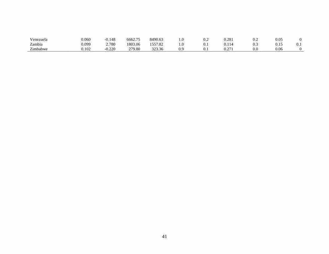
41

Venezuela 0.060 -0.148 6662.75 8490.63 1.0 0.2 0.281 0.2 0.05 0 Zambia 0.099 2.780 1803.06 1557.82 1.0 0.1 0.114 0.3 0.15 0.1 Zimbabwe 0.102 -0.220 279.80 323.36 0.9 0.1 0.271 0.0 0.06 0