On the linear programming bound for linear Lee codes · Delsarte (1973) introduced association...

Tampere University of Technology

On the linear programming bound for linear Lee codes

CitationAstola, H., & Tabus, I. (2016). On the linear programming bound for linear Lee codes. SpringerPlus, 5(1), 1-13.[246]. DOI: 10.1186/s40064-016-1863-8

Year2016

VersionPublisher's PDF (version of record)

Link to publicationTUTCRIS Portal (http://www.tut.fi/tutcris)

Published inSpringerPlus

DOI10.1186/s40064-016-1863-8

CopyrightThis article is distributed under the terms of the Creative Commons Attribution 4.0 International License(http://creativecommons.org/licenses/by/4.0/), which permits unrestricted use, distribution, and reproduction inany medium, provided you give appropriate credit to the original author(s) and the source, provide a link to theCreative Commons license, and indicate if changes were made.

Take down policyIf you believe that this document breaches copyright, please contact [email protected], and we will remove access tothe work immediately and investigate your claim.

Download date:23.07.2018

https://tutcris.tut.fi/portal/en/publications/on-the-linear-programming-bound-for-linear-lee-codes(aff6bc42-ad72-4113-a699-1d8dfb01cc1e).html

https://doi.org/10.1186/s40064-016-1863-8

On the linear programming bound for linear Lee codesHelena Astola* and Ioan Tabus

BackgroundFinding the largest code (in cardinality) with a given length and minimum distance is one of the most fundamental problems in coding theory. The most well-known upper bounds for the Hamming metric are the Hamming bound, Plotkin bound, Singleton bound and Elias bound, and these bounds have been formulated for the Lee metric also, although the expressions are slightly more complicated. Delsarte (1973) introduced association schemes to coding theory to deal with topics involving the inner distribution of a code. An important approach arises from association schemes to the problem of determining the upper bound for the size of a code, namely the linear programming approach. The asymptotically best upper bound in the Hamming metric is the McEliece–Rodemich–Rumsey–Welch bound, see McEliece et al. (1977), which is based on the linear program-ming approach, and gives a substantial improvement to the earlier best upper bound, which is the Elias bound. In the Hamming metric, the distance relations between code-words directly define an association scheme, but in the Lee metric, the distance rela-tions between the Lee-compositions define the association scheme. The Lee association scheme and linear programming bounds for Lee codes have been discussed by Astola (1982a), Solé (1988), and Tarnanen (1982). Generalizing to finite Frobenius rings, the linear programming bound for codes equipped with homogeneous weight, including the Lee weight on Z4, has been studied by Byrne et al. (2007).

Abstract

Based on an invariance-type property of the Lee-compositions of a linear Lee code, additional equality constraints can be introduced to the linear programming problem of linear Lee codes. In this paper, we formulate this property in terms of an action of the multiplicative group of the field Fq on the set of Lee-compositions. We show some useful properties of certain sums of Lee-numbers, which are the eigenvalues of the Lee association scheme, appearing in the linear programming problem of linear Lee codes. Using the additional equality constraints, we formulate the linear programming problem of linear Lee codes in a very compact form, leading to a fast execution, which allows to efficiently compute the bounds for large parameter values of the linear codes.

Keywords: Lee codes, Linear codes, Linear programming bound , Lee-compositions, Lee-numbers

Open Access

© 2016 Astola and Tabus. This article is distributed under the terms of the Creative Commons Attribution 4.0 International License (http://creativecommons.org/licenses/by/4.0/), which permits unrestricted use, distribution, and reproduction in any medium, provided you give appropriate credit to the original author(s) and the source, provide a link to the Creative Commons license, and indicate if changes were made.

RESEARCH

Astola and Tabus SpringerPlus (2016) 5:246 DOI 10.1186/s40064-016-1863-8

*Correspondence: [email protected] Department of Signal Processing, Tampere University of Technology, 33101 Tampere, Finland

http://creativecommons.org/licenses/by/4.0/

http://crossmark.crossref.org/dialog/?doi=10.1186/s40064-016-1863-8&domain=pdf

of 13Astola and Tabus SpringerPlus (2016) 5:246

We denote Znq = {x = [x1, . . . , xn]|xi ∈ {0, 1, . . . , q − 1}} the set of length n vec-

tors having q−ary elements. The Hamming distance between two vectors x, y ∈ Znq is

dH (x, y) = |{i | xi �= yi}|, and penalizes equally any non-zero error between the com-ponents of x and y, being a natural measure for errors in many communication chan-nels. However, in communication channels with phase modulation, where the symbols 0, 1, . . . , q − 1 are transmitted as phases 0, 2πq , . . . , (q − 1) 2πq , the errors are measured as the shortest distance between the symbols along the unit circle and hence we consider in the following the error between two symbols i, j ∈ Zq to be defined as the Lee distance dL(i, j) = min(|i − j|, q − |i − j|), which was introduced by Lee (1958). The Lee distance between two vectors x, y ∈ Z

nq is defined as

The Lee weight of one symbol j ∈ Zq is wL(j) = min(j, q − j) and that of one vector x ∈ Z

nq is wL(x) = dL(0, x). The number of components of the vector x ∈ Z

nq having the

Lee weight equal to i is denoted li(x) and, since li(x) = lq−i(x), only s = ⌊ q2⌋ such num-

bers describe completely the distribution of the Lee weights of the elements of x. This distribution, denoted l(x), is called the Lee-composition of x, defined as:

We denote Lnq = {t0, . . . , tα} = {l(x)|x ∈ Z

nq} the set of distinct Lee-compositions, where

(α + 1) is their number, and we reserve the notation t0 for l(0) = [n, 0, . . . , 0].A code is defined as a subset of vectors of Zn

q. Keeping with the communication scenario, only the codewords belonging to the code C are sent as messages over the communication channel, say the codeword x ∈ C is sent and is corrupted due to com-munication errors, being received as a different vector, z ∈ Z

nq. If the minimum dis-

tance d between all codewords of C is 2e + 1, then all the spheres {y|dL(x, y) ≤ e, x ∈ C} around each codeword x ∈ C are non-intersecting, and the received vector z can be correctly decoded if dL(z, x) ≤ e. When designing codes C, the minimum distance d of the code is imposed as an initial requirement. The goal is then to design a code hav-ing the largest number of codewords, so that one can send reliably as many messages as possible, with the guarantee of correcting errors of Lee weight smaller than or equal to e. Since the problem of designing the largest codes is not solved yet in general, finding upper bounds on the size of the code C for a given d is considered one of the major prob-lems in information theory. For example when new codes are proposed, comparing their size against the known upper bounds allows to prove their optimality if they achieve the upper bounds.

In the case of Lee distance, the constraints that need to be satisfied by an error cor-recting code with a given distance d can be conveniently analyzed using the associa-tion scheme introduced by Delsarte (1973). The scheme has α + 1 relations denoted Kt0 , . . . ,Ktα, where (x, y) belongs to Kti if l(x − y) = ti, with x, y ∈ Z

nq and ti ∈ Ln

q.Introduce the inner distribution of the code C as

dL(x, y) =n

∑

i=1

min(

|xi − yi|, q − |xi − yi|)

.

l(x) = [l0(x), l1(x), . . . , ls(x)].


where |C| denotes the cardinality of the set C, and in particular Bt0 = 1. Hence the desired quantity to be optimized for a code, its cardinality |C|, can be simply expressed in terms of the variables Bti as

The fundamental result of the association scheme introduced by Delsarte (1973) is the formulation of the linear constraints between the variables Bti, using as coefficients the so-called Lee-numbers, which are the eigenvalues of the Lee association scheme. Let ξ = exp(2π

√−1/q). The Lee-number Lt(u) with t,u ∈ Ln

q can be computed as follows: take any vector v having the Lee-composition u = l(v) and compute (see Astola 1982b)

The linear inequality constraints between the variables Bti are then expressed as (see Astola 1982b):

where [nk

]

=(nk

)

2n−k0 for q = 2s + 1, and (nk

)

is the multinomial coefficient ( nk0,...,ks

)

.With these constraints, the cardinality

∑

ti∈LnqBti = |C| of any code can be upper

bounded by solving a linear programming problem, as stated in the following (see Astola 1982b). Let B∗

t , t ∈ {t1, . . . , tα} be an optimal solution of the linear programming problem

where I = {i | l(x) = ti ⇒ wL(x) ≥ d}. Then 1+∑α

i=1 B∗ti is an upper bound to the size

of the code C with the minimum distance d.We have previously shown that in the case of linear Lee codes we can use the follow-

ing sharpening of the linear programming problem (see Astola and Tabus 2015). Let B∗t , t ∈ {t1, . . . , tα} be an optimal solution of the linear programming problem

Bti =1

|C||Kti ∩ C2|, ti ∈ L

nq ,

∑

ti∈Lnq

Bti = |C|.

(1)Lt(u) =∑

x|l(x)=t

(

n∏

i=1

ξ vixi

)

.

α∑

i=1

Bti Lk(ti) ≥ −[

nk

]

,

(2)

maximize

α∑

i=1

Bti

Bti ≥ 0, i ∈ I and Bti = 0, i ∈ {1, . . . ,α}\Iα∑

i=1

Bti Lk(ti) ≥ −[

nk

]

, for all k ∈ Lnq

(3)maximize

α∑

i=1

Bti

Bti ≥ 0, i ∈ I and Bti = 0, i ∈ {1, . . . ,α}\I


where τ (ti) is the set of Lee-compositions that are obtained when the vectors x having the Lee-composition ti are multiplied by all r ∈ Fq\{0}, and I = {i | l(x) = ti ⇒ wL(x) ≥ d} , i.e., the indices of those Lee-compositions corresponding to vectors of Lee weight ≥ d . Then 1+

∑αi=1 B

∗ti is an upper bound to the size of the code C with the minimum dis-

tance d.The above sharpening is based on an invariance-type property of the Lee-compositions

of a linear code. In the Hamming metric, multiplying codewords by a constant does not change the weight of the codewords. However, in the Lee metric, multiplication typically changes the Lee-composition of the codeword and so also usually the Lee weight. With linear codes, since they are linear subspaces of vector spaces, all the multiplied versions of any codeword also belong to the code. The authors have previously shown that there are as many codewords having the Lee-composition of a given codeword x as there are codewords having the Lee-composition of rx that is obtained by multiplication of the given codeword x by some constant r (see Astola and Tabus 2015).

In this paper, we formulate this property of Lee-compositions of a linear Lee code in terms of an action of the multiplicative group of the field Fq on the set of Lee-compo-sitions. This formulation gives theoretical tools for studying the Lee-compositions and linear Lee-codes. For simplicity, we let q be prime, Fn

q = {x | xi ∈ Fq , i = 1, . . . , n}. In addition, we show some useful properties of certain sums of Lee-numbers. Using the equality constraints introduced by Astola and Tabus (2015) and the properties of cer-tain sums of Lee-numbers, we may compact the set of variables and linear constraints in the linear programming problem, and perform all computations with rational numbers. Compacting the problem leads to a faster execution, which allows to efficiently compute the bounds for large parameter values.

The group actionIn the paper by Astola and Tabus (2015), a mapping τ (t) that maps the Lee-composition t into the set of Lee-compositions, which are obtained from t by multiplication of vec-tors having the Lee-composition t by all r ∈ {1, . . . , q − 1}, was defined in the following way:

where

The mapping of the Lee-compositions can be formulated in terms of a group action.

(4)Bti = Btj for all tj ∈ τ (ti)

(5)

α∑

i=1

Bti Lk(ti) ≥ −[

nk

]

, for all k ∈ Lnq

τ (t) ={[

tπr (0)(x), tπr (1)(x), . . . , tπr (s)(x)]

| t = l(x),πr(i) = |k|,kr ≡ i mod q,−s ≤ k ≤ s, 1 ≤ r ≤ q − 1

}

,

πr(i) = |k| such that rk ≡ i mod q and − s ≤ k ≤ s.


Definition 1 If G is a group and X is a set, then a group action ϕ of G on X is a function

that satisfies the following conditions for all x ∈ X:

1. ϕ(e, x) = x, where e is the identity element of G (identity).2. ϕ(g ,ϕ(h, x)) = ϕ(gh, x) for all g , h ∈ G (compatibility).For notational reasons, denote in the following the set of Lee-compositions Ln

q as {ρ(0), . . . , ρ(α)}. Now, let us define the function ϕ as follows. Denote by F∗

q the multiplica-tive group of the field Fq.

where

where

Lemma 1 The function ϕ is a group action of F∗q, where q is prime, on the set

{ρ(0), . . . , ρ(α)} of Lee-compositions.

Let us show that the above function ϕ is in fact a group action. Clearly the identity property is satisfied as

The compatibility property requires that ϕ(r1,ϕ(r2, ρ(i))) = ϕ(r1 · r2, ρ(i)), where r1, r2 ∈ F

∗q. Let us write

Then,

Now,

Therefore, we need to show that πr1(πr2(l))= πr1·r2(l).

Now,

ϕ : G × X → X

ϕ : F∗q ×

{

ρ(0), . . . , ρ(α)}

→{

ρ(0), . . . , ρ(α)}

,

ϕ(r, ρ(i)) =[

ρ(i)0 , ρ(i)

πr(1), . . . , ρ(i)

πr(s)

]

= ρ(j),

πr(l) = |k| such that rk ≡ l mod q and − s ≤ k ≤ s, r ∈ F∗q .

ϕ(1, ρ(i)) =[

ρ(i)0 , ρ

(i)1 , . . . , ρ(i)

s

]

= ρ(i).

ϕ(r2, ρ(i)) =

[

ρ(i)0 , ρ(i)

πr2(1), . . . , ρ(i)

πr2(s)

]

.

ϕ(r1, (ϕ(r2, ρ(i))) =

[

ρ(i)0 , ρ(i)

πr1

(

πr2(1)

) , . . . , ρ(i)πr1

(

πr2(s)

)

]

.

ϕ(r1 · r2, ρ(i)) =[

ρ(i)0 , ρ(i)

πr1 ·r2(1), . . . , ρ(i)

πr1·r2(s)

]

.

πr2(l) = |k1| such that r2k1 ≡ l mod q, −s ≤ k1 ≤ s,

πr1(πr2(l)) = |k2| such that r1k2 ≡ |k1| mod q, −s ≤ k2 ≤ s,

πr1r2(l) = |k3| such that r1r2k3 ≡ l mod q, −s ≤ k3 ≤ s.


We need to prove that |k2| = |k3|.

Proof We have two cases. If 1 ≤ k1 ≤ s we have

and since q is prime and −s ≤ k2, k3 ≤ s it must be that k2 = k3.If −s ≤ k1 < 0 we have

and since q is prime and −s ≤ k2, k3 ≤ s it must be that |k2| = |k3|. �

The action of F∗q on the set of Lee-compositions partitions the set into equivalence

classes, which are called orbits. So, the orbit of an element ρ(i) is

Clearly there is a correspondence between τ (ti) and the orbits Orb(ρ(i)), i.e., the sets τ (t) are the orbits of the above group action. Therefore, the theory of group actions can be used for studying the Lee-compositions and the linear programming problem, e.g., for the compact problem that we introduce in this paper, the orbit-counting theorem (see, for instance, Burnside 1897) can be used for determining the complexity of the problem as the number of orbits equals the number of variables in the compact problem.

Properties of certain sums of Lee‑numbersIn this section we study certain sums of Lee-numbers, where the Lee-numbers are taken over Lee-compositions belonging to a given orbit. We show that this type of a sum is rational as opposed to the Lee-numbers, which in many cases are irrational numbers, and that it satisfies certain equality constraints.

Since the values of the coefficients of the inner distribution are equal for all composi-tions in τ (ti), we will have in (5) sums of the form

Therefore, for each coefficient Bti we are computing a sum of Lee-numbers, where the Lee-numbers are taken over the Lee-compositions belonging to τ (ti).

Let us introduce the following lemma.

Lemma 2 Let τ (ti) = {ti1 , . . . , tiu}. Then the sum

is a rational number.

Proof First, we want to change each term Lk(ti) into Lti(k). There is the following rela-tionship between the Lee-numbers Lk(t) and Lt(k) (see Astola 1982b):

r1k2 ≡ k1 mod q ⇒ r2k1r1k2 ≡ k1l mod q ⇒ r2r1k2 ≡ l mod q,

r1k2 ≡ −k1 mod q ⇒ r2k1r1k2 ≡ −k1l mod q ⇒ r2r1(−k2) ≡ l mod q,

Orb(ρ(i)) ={

ϕ

(

r, ρ(i))

: r ∈ F∗q

}

.

Bti ·(

Lk(ti1)+ Lk(ti2)+ · · · + Lk(tiu))

.

(6)Lk(ti1)+ Lk(ti2)+ · · · + Lk(tiu),

(7)

[

nt

]

Lk(t) =[

nk

]

Lt(k),


where the coefficient [nt

]

corresponds to the number of vectors in Fnq for which the Lee-

composition is t (see Astola 1982b). Hence, we can write (6) as

Now, we notice that since all ti belong to the same τ, they are permutations of each other. This means that the coefficients

[nti

]

are all equal and (6) takes the form

where [nk

]

/[ nti1

]

= 1 if k ∈ τ (ti), and a rational number otherwise.Now, using Eq. (1), we can write the sum in parentheses above as

where u is the cardinality of τ (ti) and l(v) = k.Since the Lee-numbers Lti(k) correspond to compositions according to τ, then for each

vector x, the sum in (8) includes all the vectors rx, where r ∈ {1, . . . , q − 1}. Also, each vec-tor can only have one Lee-composition and thus can appear in only one of the sums in (8).

We may now rearrange and group the terms in (8) as

This forms a partition of the set of vectors having a Lee-composition in τ (ti), since the relation R defined as (x, y) ∈ Rx iff x = ry, r ∈ {1, . . . , q − 1} is clearly an equivalence relation.

Therefore, we can group the sum into m parts, each having q − 1 terms. We now take one such part:

and write it as

If v · xi = 0 it equals q − 1, otherwise, we have a sum of the form

So (8) is a sum of the form m1(q − 1)+m2(−1), where m1 and m2 are integers ≥ 0 such that m = m1 +m2.

Furthermore, we notice that when we look at the sums

[

nk

]

/

[

nti1

]

Lti1 (k)+[

nk

]

/

[

nti2

]

Lti2 (k)+ · · · +[

nk

]

/

[

ntiu

]

Ltiu (k).

[

nk

]

/

[

nti1

]

(

Lti1 (k)+ Lti2 (k)+ · · · + Ltiu (k))

,

(8)

Lti1 (k)+ Lti2 (k)+ · · · + Ltiu (k)

=∑

x|l(x)=ti1

(

n∏

i=1

ξ vixi

)

+∑

x|l(x)=ti2

(

n∏

i=1

ξ vixi

)

+ · · · +∑

x|l(x)=tiu

(

n∏

i=1

ξ vixi

)

(

ξ v·x1 + ξ v·2x1 + · · · + ξ v·(q−1)x1)

+(

ξ v·x2 + ξ v·2x2 + · · · + ξ v·(q−1)x2)

+ · · ·

ξ v·xi + ξ v·2xi + · · · + ξ v·(q−1)xi ,

ξ v·xi + ξ2(v·xi) + · · · + ξ (q−1)(v·xi).

ξ + ξ2 + · · · + ξq−1 = −1.

�

(9)

Lki1(ti1)+ Lki1

(ti2)+ · · · + Lki1(tiu),

Lki2(ti1)+ Lki2

(ti2)+ · · · + Lki2(tiu),

...

Lkiu′(ti1)+ Lkiu′

(ti2)+ · · · + Lkiu′(tiu),


where u is the cardinality of τ (ti) and u′ is the cardinality of τ (ki), they all turn out be equal.

Lemma 3 For ti1 , . . . , tiu ∈ τ (ti) and ki, ki′ ∈ τ (ki),

Proof First, we transform these sums using (7) into sums of the following form

Now we notice that since the Lee-compositions ki and ki′ both belong to τ (ki), the coefficients in front of the sums are all equal. What remains to show is that the sums (Lti1 (ki)+ Lti2 (ki)+ · · · + Ltiu (ki)) and (Lti1 (ki′)+ Lti2 (ki

′)+ · · · + Ltiu (ki′)) are equal. To show this, we rearrange both sums as we did in the previous proof to obtain sums of the following form. For the first sum we have

where l(v) = ki and l(xi) = ti.Now, since the Lee-compositions ki and ki′ belong to τ (ki), we obtain the vectors hav-

ing the Lee-composition ki′ from the vectors having the Lee-composition ki by multipli-cation by some r. Therefore, for the second sum we have

Now

since if v · xi = 0, they are both equal to q − 1, and otherwise each exponent is distinct. Therefore, the sums are equal. �

The compact linear programming problemThe additional equalities for linear Lee codes in (4) can be used for compacting the set of linear constraints in the linear programming problem of linear Lee codes. We enforce (3) by replacing all variables Btj for tj ∈ τ (ti) with a single variable γi, so that γi = Btj for all tj ∈ τ (ti).

We notice that by replacing the α variables Bt1 , . . . ,Btα of the linear programming problem with the set of variables γ1, . . . , γκ, where κ is the number of orbits, i.e., the number of different sets τi, we are eliminating the equality constraints from the sharp-ened linear programming problem. Let us denote by ϒ a matrix, where we have listed all the Lee-numbers as

Lki(ti1)+ Lki(ti2)+ · · · + Lki(tiu) = Lki′ (ti1)+ Lki′ (ti2)+ · · · + Lki′ (tiu).

[

nki

]

/

[

nti1

]

(

Lti1 (ki)+ Lti2 (ki)+ · · · + Ltiu (ki))

,

[

nki′

]

/

[

nti1

]

(

Lti1 (ki′)+ Lti2 (ki

′)+ · · · + Ltiu (ki′))

.

(

ξ v·x1 + ξ2(v·x1) + · · · + ξ (q−1)v·x1)

+(

ξ v·x2 + ξ2(v·x2) + · · · + ξ (q−1)v·x2)

+ · · · ,

(

ξ rv·x1 + ξ r2(v·x1) + · · · + ξ r(q−1)v·x1)

+(

ξ rv·x2 + ξ r2(v·x2) + · · · + ξ r(q−1)v·x2)

+ · · · .

ξ v·xi + ξ2(v·xi) + · · · + ξ (q−1)v·xi = ξ rv·xi + ξ r2(v·xi) + · · · + ξ r(q−1)v·xi ,


Let A be an α × κ matrix of the form

where the number of rows inside each partition corresponds to the cardinalities of the sets τi.

We introduce the vector γ = (γ0, γ1, . . . , γκ) and formulate the linear programming problem equivalent to (3):

where I = {i | ∀t ∈ τi : l(x) = t ⇒ wL(x) ≥ d}, i.e., the indices of those sets τi, where all Lee-compositions correspond to vectors of Lee weight ≥ d.

The cardinalities |τi| appear in the criterion of the problem since the initial criterion expressed in terms of the variables Bt1 , . . . ,Btα is 1TB, where 1 is the all one vector and B = [Bt1 , . . . ,Btα ]T, and the criterion in the new variables is 1TAγ, where the new vector of coefficients, 1TA, will have as elements the size of the partitions of A, which are equal to the cardinalities of the sets τi.

Additionally we notice that the matrix U = ϒA can be seen to have the partition structure similar to that of A,

ϒ =

Lk0(t0) Lk0(t1) · · · Lk0(tα)Lk1(t0) Lk1(t1) · · · Lk1(tα)

.... . .

...

Lkα (t0) Lkα (t1) · · · Lkα (tα)

A =

1 0 0 0 · · · 0

0 1 0 0 · · · 0

0 1 0 0 · · · 0

0 1 0 0 · · · 0

0 1 0 0 · · · 0

0 0 1 0 · · · 0

0 0 1 0 · · · 0

· · ·0 0 0 0 · · · 1

,

maximize

κ∑

i=1

|τi|γi

γ0 = 1 and γi ≥ 0, i ∈ I and γi = 0, i ∈ {1, . . . ,α}\IϒAγ ≥ 0,

U = ϒA = ϒ

1 0 0 0 · · · 0

0 1 0 0 · · · 0

0 1 0 0 · · · 0

0 1 0 0 · · · 0

0 1 0 0 · · · 0

0 0 1 0 · · · 0

0 0 1 0 · · · 0

· · ·0 0 0 0 · · · 1

=

�1,1 �1,2 �1,3 �1,4 · · · �1,κ

�2,1 �2,2 �2,3 �2,4 · · · �2,κ

�2,1 �2,2 �2,3 �2,4 · · · �2,κ

�2,1 �2,2 �2,3 �2,4 · · · �2,κ

�2,1 �2,2 �2,3 �2,4 · · · �2,κ

�3,1 �3,2 �3,3 �3,4 · · · �3,κ

�3,1 �3,2 �3,3 �3,4 · · · �3,κ

· · ·�κ ,1 �κ ,2 �κ ,3 �κ ,4 · · · �κ ,κ

= A�


where the matrix � = [�]i,j is κ × κ and the rows in a partition correspond to the Lee-compositions belonging to the same set τi. Inside a partition the rows of the matrix U are identical, due to Lemma 3, since the columns of U inside a partition have the following elements

where |τki | = u′ and |τti | = u. This leads to a repeated inequality constraint. In order to remove this redundancy, we select from the matrix U only one row per partition block, keeping thus only the non-redundant inequalities. This is just the matrix �, and we may replace the inequality constraints ϒAγ ≥ 0 with �γ ≥ 0. In addition, due to Lemma 2, each element of � is a rational number, and the Lee-numbers can be computed recur-sively with integers using the recursive formula given by Astola and Tabus (2013). Hence, we can perform all computations using integers instead of irrationals.

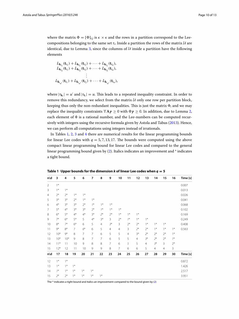
In Tables 1, 2, 3 and 4 there are numerical results for the linear programming bounds for linear Lee codes with q = 5, 7, 13, 17. The bounds were computed using the above compact linear programming bound for linear Lee codes and compared to the general linear programming bound given by (2). Italics indicates an improvement and * indicates a tight bound.

Lki1(ti1)+ Lki1

(ti2)+ · · · + Lki1(tiu),

Lki2(ti1)+ Lki2

(ti2)+ · · · + Lki2(tiu),

...

Lkiu′(ti1)+ Lkiu′

(ti2)+ · · · + Lkiu′(tiu),

Table 1 Upper bounds for the dimension k of linear Lee codes when q = 5

The * indicates a tight bound and italics an improvement compared to the bound given by (2)

n\d 3 4 5 6 7 8 9 10 11 12 13 14 15 16 Time [s]

2 1* 0.007

3 1* 1* 0.013

4 2* 2* 1* 1* 0.026

5 3* 3* 2* 1* 1* 0.041

6 4* 3* 3* 2* 1* 1* 1* 0.068

7 5* 4* 3* 3* 2* 1* 1* 1* 0.102

8 6* 5* 4* 4* 3* 2* 2* 1* 1* 1* 0.169

9 7* 6* 5* 5 4* 3* 3 2* 1* 1* 1* 0.249

10 8* 7* 6* 6 5 4 3* 3 2* 2* 1* 1* 1* 0.408

11 9* 8* 7 6* 6 5 4 4 3 2* 2* 1* 1* 1* 0.563

12 10* 9* 8 7 7 6 5 5 4 3* 2* 2* 2* 1*

13 10* 10* 9 8 7 7 6 5 5 4 3* 2* 2* 1*

14 11* 11 10 9 8 8 7 6 5 5 4 3* 3 2*

15 12* 12 11 10 9 9 8 7 6 6 5 4 4 3

n\d 17 18 19 20 21 22 23 24 25 26 27 28 29 30 Time [s]

12 1* 1* 0.872

13 1* 1* 1* 1.426

14 1* 1* 1* 1* 1* 2.517

15 2* 2* 1* 1* 1* 1* 3.951


In Tables 1, 2, 3 and 4, the computation time is also shown for each n. When com-puting the sharpened linear programming bound by giving additional equality con-straints to the linear programming solver, more computation time is required for given parameters than with the general linear programming problem given by (2), since the



n\d 3 4 5 6 7 8 9 10 11 12 13 14 15 16 Time [s]

2 1* 0.009

3 2* 1* 1* 1* 0.028

4 2* 2* 2* 1* 1* 0.047

5 3* 3* 2* 2* 1* 1* 1* 0.098

6 4* 4* 3* 3* 2* 2* 1* 1* 1* 1* 0.212

7 5* 5* 4* 4 3* 3 2* 2* 1* 1* 1* 0.420

8 6* 5* 5* 4* 4* 4 3* 3 2* 2* 1* 1* 1* 0.816

9 7* 6* 6 5* 5 4* 4 3* 3 3 2* 1* 1* 1*

10 8* 7* 7 6* 6 5 5 4 4 3* 3 2* 2* 1*

11 9* 8* 8 7 6* 5 5 5 5 4 4 3 3 2*

12 10* 9* 8* 8 7 7 6 6 5 5 4 4 3 3

13 11* 10* 9* 9 8 8 7 7 6 6 5 5 4 4

14 12* 11* 10* 10 9 9 8 8 7 7 6 6 5 5

15 13* 12* 11* 11 10 10 9 9 8 7 7 6 6 5

n\d 17 18 19 20 21 22 23 24 25 26 27 28 29 30 Time [s]

9 1* 1* 1.621

10 1* 1* 1* 2.959

11 2* 2 1* 1* 1* 6.406

12 3 2* 2 1* 1* 1* 1* 1* 17.580

13 3 3 2* 2* 2 1* 1* 1* 1* 31.983

14 4 4 3 3 2* 2* 2 1* 1* 1* 1* 67.885

15 5 5 4 4 3 3 2* 2* 1* 1* 1* 1* 1* 1* 173.448



n\d 3 4 5 6 7 8 9 10 11 12 13 14 15 16 Time [s]

2 1* 1* 1* 0.038

3 2* 1* 1* 1* 1* 1* 1 0.107

4 3* 2* 2* 2* 2* 1* 1* 1* 1* 1* 1 0.487

5 4* 3* 3* 3 2* 2* 2* 2 1* 1* 1* 1* 1* 1

6 5* 4* 4* 3* 3* 3* 3 2* 2* 2* 2 1* 1* 1*

7 5* 5* 5 4* 4* 4 3* 3* 3* 3 2* 2* 2* 2*

8 6* 6* 6 5* 5 5 4* 4 4 3* 3* 3 3 2*

n\d 17 18 19 20 21 22 23 24 25 26 27 28 29 30 Time [s]

5 1 2.288

6 1* 1* 1* 1* 1* 11.508

7 2 1* 1* 1* 1* 1* 57.325

8 2* 2* 2* 2 2 1* 1* 1* 1* 1* 300.543


linear programming solver is given a larger set of overall constraints. However, using the compact problem introduced in this paper reduces the computation time significantly, since there are less variables and constraints and all computations can be performed with rational numbers. For example, on an Apple iMac 5K (late 2014) with Intel Core i7 (I7-4790K), 32 gigabytes of memory, and a 64-bit operating system OS X Yosemite, and using the linprog linear programming solver of Matlab, for q = 17 and n = 5, com-puting the regular linear programming bounds took approximately 17 min and comput-ing the sharpened bounds by using additional equality constraints took over 5 h. When using the compact problem, the computation time was less than 20 s, including compu-tation of the new sets of constraints from the Lee-numbers according to the sets τ (t), which is a significant improvement and makes it possible to compute the bounds for larger parameter values in a reasonable time. The Lee-numbers were computed sepa-rately, and computing them recursively for q = 17 and n = 2, . . . , 6 took approximately 1 min.

The obtained bounds can be used for identifying optimal codes. Consider the bound for k given in Table 4 with q = 17, n = 5 and d = 7, which is 2. This means that the maxi-mum number of codewords in a linear code with these parameters is at most 289. The code having the generator matrix

is a [5, 2]-code with the minimum distance 7 and has 172 = 289 codewords, therefore, it is an optimal linear code for the above parameters.

ConclusionsIn this paper, we formulated the invariance-type property of Lee-compositions intro-duced by Astola and Tabus (2015) in terms of an action of the multiplicative group of the field Fq on the set of Lee-compositions. This formulation is useful in the theoretical study of Lee-compositions and linear Lee codes. In addition, we have shown some useful properties of certain sums of Lee-numbers that appear in the constraints of the linear programming problem of linear Lee codes. Based on the equality constraints and these properties, we constructed a more compact linear programming problem for linear Lee codes, leading to a fast execution and allowing all computations to be performed using

G =[

1 0 5 0 4

0 1 16 15 10

]


The ∗ indicates a tight bound and italics an improvement compared to the bound given by (2)

n\d 3 4 5 6 7 8 9 10 11 12 13 14 15 16 Time [s]

2 1* 1* 1* 0.043

3 2* 2* 1* 1* 1* 1* 1* 0.276

4 3* 2* 2* 2* 2* 2* 1* 1* 1* 1* 1* 1* 1* 2.271

5 4* 3* 3* 3* 2* 2* 2* 2* 2* 2 1* 1* 1* 1*

6 5* 4* 4* 4* 3* 3* 3* 3 2* 2* 2* 2* 2* 2*

n\d 17 18 19 20 21 22 23 24 25 26 27 28 29 30 Time [s]

5 1* 1* 1* 19.117

6 1* 1* 1* 1* 1* 1* 1* 1* 188.785


integers. This leads in practice to having available upper bounds for codes with param-eters higher than available up to now.Authors’ contributionsBoth authors read and approved the final manuscript.

Competing interestsThe authors declare that they have no competing interests.

Received: 29 October 2015 Accepted: 16 February 2016

ReferencesAstola H, Tabus I (2013) Bounds on the size of Lee-codes. In: 8thInternational symposium on image and signal processing

and analysis,Trieste, Italy, pp 464–469Astola H, Tabus I (2015) Sharpening the linear programming bound for linear Lee-codes. Electron Lett 51(6):492–494.

doi:10.1049/el.2014.4300Astola J (1982a) The Lee-scheme and bounds for Lee-codes. Cybern Syst 13(4):331–343. doi:10.1080/01969728208927711Astola J (1982b) The theory of Lee-codes. Lappeenranta University of Technology, Department of Physics and Mathemat-

ics, Research Report 1/1982Burnside W (1897) Theory of groups of finite order. Cambridge University Press, CambridgeByrne E, Greferath M, O’Sullivan ME (2007) The linear programming bound for codes over finite Frobenius rings. Des

Codes Cryptogr 42(3):289–301Delsarte P (1973) An algebraic approach to the association schemes of coding theory. Philips research reports: Supple-

ments 10Lee CY (1958) Some properties of nonbinary error-correcting codes. IRE Trans Inf Theory 4(2):77–82McEliece R, Rodemich E, Rumsey H, Welch L (1977) New upper bounds on the rate of a code via the Delsarte–MacWil-

liams inequalities. IEEE Trans Inf Theory 23(2):157–166Solé P (1988) The Lee association scheme. In: Cohen G, Godlewski P (eds) Coding theory and applications. Lecture notes

in Computer science, vol 311. Springer, Berlin, pp 45–55. doi:10.1007/3-540-19368-5_5Tarnanen H (1982) An approach to constant weight and Lee codes by using the methods of association schemes.

Publications of University of Turku: Annales universitatis turkuensis. Series A I: Astronomica-chemica-physica-mathe-matica. University of Turku, Turku

http://dx.doi.org/10.1049/el.2014.4300

http://dx.doi.org/10.1080/01969728208927711

http://dx.doi.org/10.1007/3-540-19368-5_5

On the linear programming bound for linear Lee codes · Delsarte (1973) introduced association...

Documents

Transcript of On the linear programming bound for linear Lee codes · Delsarte (1973) introduced association...