1

On the linear convergence of distributedoptimization over directed graphs

Chenguang Xi, and Usman A. Khan†

Abstract—This paper develops a fast distributed algorithm,termed DEXTRA, to solve the optimization problem when nagents reach agreement and collaboratively minimize the sum oftheir local objective functions over the network, where the com-munication between the agents is described by a directed graph.Existing algorithms solve the problem restricted to directedgraphs with convergence rates of O(ln k/

√k) for general convex

objective functions and O(ln k/k) when the objective functionsare strongly-convex, where k is the number of iterations. We showthat, with the appropriate step-size, DEXTRA converges at alinear rate O(τk) for 0 < τ < 1, given that the objective functionsare restricted strongly-convex. The implementation of DEXTRArequires each agent to know its local out-degree. Simulationexamples further illustrate our findings.

Index Terms—Distributed optimization; multi-agent networks;directed graphs.

I. INTRODUCTION

Distributed computation and optimization have gained greatinterests due to their widespread applications in, e.g., large-scale machine learning, [1, 2], model predictive control, [3],cognitive networks, [4, 5], source localization, [6, 7], resourcescheduling, [8], and message routing, [9]. All of these applica-tions can be reduced to variations of distributed optimizationproblems by a network of agents when the knowledge ofobjective functions is distributed over the network. In par-ticular, we consider the problem of minimizing a sum ofobjectives,

∑ni=1 fi(x), where fi : Rp → R is a private

objective function at the ith agent of the network.There are many algorithms to solve the above problem in a

distributed manner. A few notable approaches are DistributedGradient Descent (DGD), [10, 11], Distributed Dual Averag-ing (DDA), [12], and the distributed implementations of theAlternating Direction Method of Multipliers (ADMM), [13–15]. The algorithms, DGD and DDA, are essentially gradient-based, where at each iteration a gradient-related step is cal-culated, followed by averaging over the neighbors in the net-work. The main advantage of these methods is computationalsimplicity. However, their convergence rate is slow due tothe diminishing step-size, which is required to ensure exactconvergence. The convergence rate of DGD and DDA witha diminishing step-size is shown to be O( ln k√

k), [10]; under

a constant step-size, the algorithm accelerates to O( 1k ) at

the cost of inexact convergence to a neighborhood of theoptimal solution, [11]. To overcome such difficulties, some

†C. Xi and U. A. Khan are with the Department of Electrical and Com-puter Engineering, Tufts University, 161 College Ave, Medford, MA 02155;chenguang.xi@tufts.edu, khan@ece.tufts.edu. This work hasbeen partially supported by an NSF Career Award # CCF-1350264.

alternate approaches include the Nesterov-based methods,e.g., Distributed Nesterov Gradient (DNG) with a conver-gence rate of O( ln k

k ), and Distributed Nesterov gradient withConsensus iterations (DNC), [16]. The algorithm, DNC, canbe interpreted to have an inner loop, where information isexchanged, within every outer loop where the optimization-step is performed. The time complexity of the outer loopis O( 1

k2 ) whereas the inner loop performs a substantial O(ln k)information exchanges within the kth outer loop. Therefore,the equivalent convergence rate of DNC is O( ln k

k2 ). Both DNGand DNC assume the gradient to be bounded and Lipschitzcontinuous at the same time. The discussion of convergencerate above applies to general convex functions. When theobjective functions are further strongly-convex, DGD andDDA have a faster convergence rate of O( ln k

k ), and DGDwith a constant step-size converges linearly to a neighborhoodof the optimal solution. See Table I for a comparison of relatedalgorithms.

Other related algorithms include the distributed implemen-tation of ADMM, based on augmented Lagrangian, whereat each iteration the primal and dual variables are solved tominimize a Lagrangian-related function, [13–15]. Comparingto the gradient-based methods with diminishing step-sizes, thistype of method converges exactly to the optimal solution witha faster rate of O( 1

k ) owing to the constant step-size; andfurther has a linear convergence when the objective functionsare strongly-convex. However, the disadvantage is a highcomputation burden because each agent needs to optimize asubproblem at each iteration. To resolve this issue, Decentral-ized Linearized ADMM (DLM), [17], and EXTRA, [18], areproposed, which can be considered as a first-order approxima-tion of decentralized ADMM. DLM and EXTRA converge at alinear rate if the local objective functions are strongly-convex.All these distributed algorithms, [10–19], assume the multi-agent network to be an undirected graph. In contrast, literatureconcerning directed graphs is relatively limited. The challengelies in the imbalance caused by the asymmetric informationexchange in directed graphs.

We report the papers considering directed graphs here.Broadly, there are three notable approaches, which are allgradient-based algorithms with diminishing step-sizes. Thefirst is called Gradient-Push (GP), [20–23], which combinesgradient-descent and push-sum consensus. The push-sum al-gorithm, [24, 25], is first proposed in consensus problems toachieve average-consensus1 in a directed graph, i.e., with acolumn-stochastic matrix. The idea is based on computing

1See [26–29], for additional information on average-consensus problems.

2

the stationary distribution of the column-stochastic matrixcharacterized by the underlying multi-agent network andcanceling the imbalance by dividing with the right eigen-vector of the column-stochastic matrix. Directed-DistributedGradient Descent (D-DGD), [30, 31], follows the idea ofCai and Ishii’s work on average-consensus, [32], where anew non-doubly-stochastic matrix is constructed to reachaverage-consensus. The underlying weighting matrix containsa row-stochastic matrix as well as a column-stochastic ma-trix, and provides some nice properties similar to doubly-stochastic matrices. In [33], where we name the methodWeight-Balancing-Distributed Gradient Descent (WB-DGD),the authors combine the weight-balancing technique, [34],together with gradient-descent. These gradient-based meth-ods, [20–23, 30, 31, 33], restricted by the diminishing step-size, converge relatively slow at O( ln k√

k). Under strongly-

convex objective functions, the convergence rate of GP canbe accelerated to O( ln k

k ), [35]. We sum up the existing first-order distributed algorithms and provide a comparison in termsof speed, in Table I, including both undirected and directedgraphs. In Table I, ‘I’ means DGD with a constant step-sizeis an Inexact method, and ‘C’ represents that DADMM has amuch higher Computation burden compared to other first-ordermethods.

Algorithms General Convex strongly-convex

undirected

DGD (αk) O( ln k√k) O( ln k

k)

DDA (αk) O( ln k√k) O( ln k

k)

DGD (α) (I) O( 1k) O(τk)

DNG (αk) O( ln kk

)

DNC (α) O( ln kk2

)

DADMM (α) (C) O(τk)

DLM (α) O(τk)

EXTRA (α) O( 1k) O(τk)

directed

GP (αk) O( ln k√k) O( ln k

k)

D-DGD (αk) O( ln k√k) O( ln k

k)

WB-DGD (αk) O( ln k√k) O( ln k

k)

DEXTRA (α) O(τk)

TABLE I: Convergence rate of first-order distributed optimization algorithmsregarding undirected and directed graphs.

In this paper, we propose a fast distributed algorithm, termedDEXTRA, to solve the corresponding distributed optimizationproblem over directed graphs. We assume that the objectivefunctions are restricted strongly-convex, a relaxed versionof strong-convexity, under which we show that DEXTRAconverges linearly to the optimal solution of the problem.DEXTRA combines the push-sum protocol and EXTRA. Thepush-sum protocol has been proven useful in dealing withoptimization over digraphs, [20–23], while EXTRA workswell in optimization problems over undirected graphs witha fast convergence rate and a low computation complexity.By integrating the push-sum technique into EXTRA, we showthat DEXTRA converges exactly to the optimal solution witha linear rate, O(τk), when the underlying network is directed.Note that O(τk) is commonly described as linear and it should

be interpreted as linear on a log-scale. The fast convergencerate is guaranteed because DEXTRA has a constant step-size compared with the diminishing step-size used in GP,D-DGD, or WB-DGD. Currently, our formulation is limitedto restricted strongly-convex functions. Finally, we note thatan earlier version of DEXTRA, [36], was used in [37] todevelop Normalized EXTRAPush. Normalized EXTRAPushimplements the DEXTRA iterations after computing the righteigenvector of the underlying column-stochastic, weightingmatrix; this computation requires either the knowledge ofthe weighting matrix at each agent, or, an iterative algorithmthat converges asymptotically to the right eigenvector. Clearly,DEXTRA does not assume such knowledge.

The remainder of the paper is organized as follows. Sec-tion II describes, develops, and interprets the DEXTRA al-gorithm. Section III presents the appropriate assumptions andstates the main convergence results. In Section IV, we presentsome lemmas as the basis of the proof of DEXTRA’s conver-gence. The main proof of the convergence rate of DEXTRAis provided in Section V. We show numerical results inSection VI and Section VII contains the concluding remarks.

Notation: We use lowercase bold letters to denote vectorsand uppercase italic letters to denote matrices. We denoteby [x]i, the ith component of a vector, x. For a matrix, A,we denote by [A]i, the ith row of A, and by [A]ij , the (i, j)thelement of A. The matrix, In, represents the n × n identity,and 1n and 0n are the n-dimensional vector of all 1’s and0’s. The inner product of two vectors, x and y, is 〈x,y〉. TheEuclidean norm of any vector, x, is denoted by ‖x‖. We definethe A-matrix norm, ‖x‖2A, of any vector, x, as

‖x‖2A , 〈x, Ax〉 = 〈x, A>x〉 = 〈x, A+A>

2x〉,

where A is not necessarily symmetric. Note that the A-matrix norm is non-negative only when A + A> is PositiveSemi-Definite (PSD). If a symmetric matrix, A, is PSD, wewrite A � 0, while A � 0 means A is Positive Definite (PD).The largest and smallest eigenvalues of a matrix A are denotedas λmax(A) and λmin(A). The smallest nonzero eigenvalueof a matrix A is denoted as λmin(A). For any f(x), ∇f(x)denotes the gradient of f at x.

II. DEXTRA DEVELOPMENT

In this section, we formulate the optimization problem anddescribe DEXTRA. We first derive an informal but intuitiveproof showing that DEXTRA pushes the agents to achieveconsensus and reach the optimal solution. The EXTRA algo-rithm, [18], is briefly recapitulated in this section. We deriveDEXTRA to a similar form as EXTRA such that our algorithmcan be viewed as an improvement of EXTRA suited to the caseof directed graphs. This reveals the meaning behind DEXTRA:Directed EXTRA. Formal convergence results and proofs areleft to Sections III, IV, and V.

Consider a strongly-connected network of n agents com-municating over a directed graph, G = (V, E), where Vis the set of agents, and E is the collection of orderedpairs, (i, j), i, j ∈ V , such that agent j can send informationto agent i. Define N in

i to be the collection of in-neighbors,

3

i.e., the set of agents that can send information to agent i.Similarly, N out

i is the set of out-neighbors of agent i. We allowbothN in

i andN outi to include the node i itself. Note that in a di-

rected graph when (i, j) ∈ E , it is not necessary that (j, i) ∈ E .Consequently, N in

i 6= N outi , in general. We focus on solving

a convex optimization problem that is distributed over theabove multi-agent network. In particular, the network of agentscooperatively solve the following optimization problem:

P1 : min f(x) =

n∑i=1

fi(x),

where each local objective function, fi : Rp → R, is convexand differentiable, and known only by agent i. Our goal is todevelop a distributed iterative algorithm such that each agentconverges to the global solution of Problem P1.

A. EXTRA for undirected graphs

EXTRA is a fast exact first-order algorithm that solveProblem P1 when the communication network is undirected.At the kth iteration, agent i performs the following update:

xk+1i =xki +

∑j∈Ni

wijxkj −

∑j∈Ni

wijxk−1j

− α[∇fi(xki )−∇fi(xk−1

i )], (1)

where the weights, wij , form a weighting matrix, W = {wij},that is symmetric and doubly-stochastic. The collection W ={wij} satisfies W = θIn + (1 − θ)W , with some θ ∈ (0, 1

2 ].The update in Eq. (1) converges to the optimal solution ateach agent i with a convergence rate of O( 1

k ) and convergeslinearly when the objective functions are strongly-convex. Tobetter represent EXTRA and later compare with DEXTRA,we write Eq. (1) in a matrix form. Let xk, ∇f(xk) ∈ Rnpbe the collections of all agent states and gradients at time k,i.e., xk , [xk1 ; · · · ;xkn], ∇f(xk) , [∇f1(xk1); · · · ;∇fn(xkn)],and W , W ∈ Rn×n be the weighting matrices collectingweights, wij , wij , respectively. Then, Eq. (1) can be repre-sented in a matrix form as:

xk+1 = [(In +W )⊗ Ip]xk − (W ⊗ Ip)xk−1

− α[∇f(xk)−∇f(xk−1)

], (2)

where the symbol ⊗ is the Kronecker product. We now stateDEXTRA and derive it in a similar form as EXTRA.

B. DEXTRA Algorithm

To solve the Problem P1 suited to the case of directedgraphs, we propose DEXTRA that can be described as follows.Each agent, j ∈ V , maintains two vector variables: xkj , zkj ∈Rp, as well as a scalar variable, ykj ∈ R, where k is thediscrete-time index. At the kth iteration, agent j weights itsstates, aijxkj , aijykj , as well as aijxk−1

j , and sends these toeach of its out-neighbors, i ∈ N out

j , where the weights, aij ,and, aij ,’s are such that:

aij =

> 0, i ∈ N outj ,

0, otw.,

n∑i=1

aij = 1,∀j, (3)

aij =

θ + (1− θ)aij , i = j,

(1− θ)aij , i 6= j,∀j, (4)

where θ ∈ (0, 12 ]. With agent i receiving the information

from its in-neighbors, j ∈ N ini , it calculates the state, zki , by

dividing xki over yki , and updates xk+1i and yk+1

i as follows:

zki =xkiyki, (5a)

xk+1i =xki +

∑j∈N in

i

(aijx

kj

)−∑j∈N in

i

(aijx

k−1j

)− α

[∇fi(zki )−∇fi(zk−1

i )], (5b)

yk+1i =

∑j∈N in

i

(aijy

kj

). (5c)

In the above, ∇fi(zki ) is the gradient of the function fi(z)at z = zki , and ∇fi(zk−1

i ) is the gradient at zk−1i , respectively.

The method is initiated with an arbitrary vector, x0i , and

with y0i = 1 for any agent i. The step-size, α, is a positive

number within a certain interval. We will explicitly discussthe range of α in Section III. We adopt the conventionthat x−1

i = 0p and ∇fi(z−1i ) = 0p, for any agent i, such

that at the first iteration, i.e., k = 0, we have the followingiteration instead of Eq. (5),

z0i =

x0i

y0i

, (6a)

x1i =

∑j∈N in

i

(aijx

0j

)− α∇fi(z0

i ), (6b)

y1i =

∑j∈N in

i

(aijy

0j

). (6c)

We note that the implementation of Eq. (5) needs each agentto have the knowledge of its out-neighbors (such that it candesign the weights according to Eqs. (3) and (4)). In a morerestricted setting, e.g., a broadcast application where it maynot be possible to know the out-neighbors, we may use aij =|N out

j |−1; thus, the implementation only requires each agentto know its out-degree, [20–23, 30, 31, 33].

To simplify the proof, we write DEXTRA, Eq. (5), in a ma-trix form. Let, A = {aij} ∈ Rn×n, A = {aij} ∈ Rn×n, be thecollection of weights, aij , aij , respectively. It is clear that bothA and A are column-stochastic matrices. Let xk, zk,∇f(xk) ∈Rnp, be the collection of all agent states and gradients attime k, i.e., xk , [xk1 ; · · · ;xkn], zk , [zk1 ; · · · ; zkn], ∇f(xk) ,[∇f1(xk1); · · · ;∇fn(xkn)], and yk ∈ Rn be the collection ofagent states, yki , i.e., yk , [yk1 ; · · · ; ykn]. Note that at time k,yk can be represented by the initial value, y0:

yk = Ayk−1 = Aky0 = Ak · 1n. (7)

Define a diagonal matrix, Dk ∈ Rn×n, for each k, such thatthe ith element of Dk is yki , i.e.,

Dk = diag(yk)

= diag(Ak · 1n

). (8)

Given that the graph, G, is strongly-connected and the cor-responding weighting matrix, A, is non-negative, it follows

4

that Dk is invertible for any k. Then, we can write Eq. (5) inthe matrix form equivalently as follows:

zk =([Dk]−1 ⊗ Ip

)xk, (9a)

xk+1 =xk + (A⊗ Ip)xk − (A⊗ Ip)xk−1

− α[∇f(zk)−∇f(zk−1)

], (9b)

yk+1 =Ayk, (9c)

where both of the weight matrices, A and A, are column-stochastic and satisfy the relationship: A = θIn + (1 − θ)Awith some θ ∈ (0, 1

2 ]. From Eq. (9a), we obtain for any k

xk =(Dk ⊗ Ip

)zk. (10)

Therefore, Eq. (9) can be represented as a single equation:(Dk+1 ⊗ Ip

)zk+1 =

[(In +A)Dk ⊗ Ip

]zk

− (ADk−1 ⊗ Ip)zk−1 − α[∇f(zk)−∇f(zk−1)

]. (11)

We refer to the above algorithm as DEXTRA, since Eq. (11)has a similar form as EXTRA in Eq. (2) and is designed tosolve Problem P1 in the case of directed graphs. We state ourmain result in Section III, showing that as time goes to infinity,the iteration in Eq. (11) pushes zk to achieve consensus andreach the optimal solution in a linear rate. Our proof in thispaper will based on the form, Eq. (11), of DEXTRA.

C. Interpretation of DEXTRA

In this section, we give an intuitive interpretation onDEXTRA’s convergence to the optimal solution; the formalproof will appear in Sections IV and V. Since A is column-stochastic, the sequence,

{yk}

, generated by Eq. (9c), satisfieslimk→∞ yk = π, where π is some vector in the span of A’sright-eigenvector corresponding to the eigenvalue 1. We alsoobtain that D∞ = diag (π). For the sake of argument, letus assume that the sequences,

{zk}

and{xk}

, generated byDEXTRA, Eq. (9) or (11), also converge to their own lim-its, z∞ and x∞, respectively (not necessarily true). Accordingto the updating rule in Eq. (9b), the limit x∞ satisfies

x∞ =x∞ + (A⊗ Ip)x∞ − (A⊗ Ip)x∞

− α [∇f(z∞)−∇f(z∞)] , (12)

which implies that [(A− A)⊗ Ip]x∞ = 0np, or x∞ = π⊗ufor some vector, u ∈ Rp. It follows from Eq. (9a) that

z∞ =(

[D∞]−1 ⊗ Ip

)(π ⊗ u) = 1n ⊗ u, (13)

where the consensus is reached. The above analysis revealsthe idea of DEXTRA, which is to overcome the imbalanceof agent states occurred when the graph is directed: both x∞

and y∞ lie in the span of π; by dividing x∞ over y∞, theimbalance is canceled.

Summing up the updates in Eq. (9b) over k from 0 to ∞,we obtain that

x∞ = (A⊗ Ip)x∞ − α∇f(z∞)−∞∑r=0

[(A−A

)⊗ Ip

]xr;

note that the first iteration is slightly different as shown inEqs. (6). Consider x∞ = π⊗u and the preceding relation. Itfollows that the limit, z∞, satisfies

α∇f(z∞) = −∞∑r=0

[(A−A

)⊗ Ip

]xr. (14)

Therefore, we obtain that

α (1n ⊗ Ip)>∇f(z∞) = −[1>n

(A−A

)⊗ Ip

] ∞∑r=0

xr = 0p,

which is the optimality condition of Problem P1 consideringthat z∞ = 1n ⊗ u. Therefore, given the assumption thatthe sequence of DEXTRA iterates,

{zk}

and{xk}

, havelimits, z∞ and x∞, we have the fact that z∞ achievesconsensus and reaches the optimal solution of Problem P1.In the next section, we state our main result of this paper andwe defer the formal proof to Sections IV and V.

III. ASSUMPTIONS AND MAIN RESULTS

With appropriate assumptions, our main result states thatDEXTRA converges to the optimal solution of Problem P1linearly. In this paper, we assume that the agent graph, G,is strongly-connected; each local function, fi : Rp → R, isconvex and differentiable, and the optimal solution of ProblemP1 and the corresponding optimal value exist. Formally, wedenote the optimal solution by u ∈ Rp and optimal valueby f∗, i.e.,

f∗ = f(u) = minx∈Rp

f(x). (15)

Let z∗ ∈ Rnp be defined as

z∗ = 1n ⊗ u. (16)

Besides the above assumptions, we emphasize some otherassumptions regarding the objective functions and weightingmatrices, which are formally presented as follows.

Assumption A1 (Functions and Gradients). Each privatefunction, fi, is convex and differentiable and satisfies thefollowing assumptions.(a) The function, fi, has Lipschitz gradient with the con-

stant Lfi , i.e., ‖∇fi(x)−∇fi(y)‖ ≤ Lfi‖x−y‖, ∀x,y ∈Rp.

(b) The function, fi, is restricted strongly-convex2 with re-spect to point u with a positive constant Sfi , i.e., Sfi‖x−u‖2 ≤ 〈∇fi(x)−∇fi(u),x− u〉, ∀x ∈ Rp, where u isthe optimal solution of the Problem P1.

Following Assumption A1, we have for any x,y ∈ Rnp,

‖∇f(x)−∇f(y)‖ ≤ Lf ‖x− y‖ , (17a)

Sf ‖x− z∗‖2 ≤ 〈∇f(x)−∇f(z∗),x− z∗〉 , (17b)

where the constants Lf = maxi{Lfi}, Sf = mini{Sfi}, and∇f(x) , [∇f1(x1); · · · ;∇fn(xn)] for any x , [x1; · · · ;xn].

2There are different definitions of restricted strong-convexity. We use thesame as the one used in EXTRA, [18].

5

Recall the definition of Dk in Eq. (8), we formally denotethe limit of Dk by D∞, i.e.,

D∞ = limk→∞

Dk = diag (A∞ · 1n) = diag (π) , (18)

where π is some vector in the span of the right-eigenvectorof A corresponding to eigenvalue 1. The next assumption isrelated to the weighting matrices, A, A, and D∞.

Assumption A2 (Weighting matrices). The weighting matri-ces, A and A, used in DEXTRA, Eq. (9) or (11), satisfy thefollowing.

(a) A is a column-stochastic matrix.(b) A is a column-stochastic matrix and satisfies A = θIn +

(1− θ)A, for some θ ∈ (0, 12 ].

(c) (D∞)−1A+ A> (D∞)

−1 � 0.

One way to guarantee Assumption A2(c) is to design theweighting matrix, A, to be diagonally-dominant. For example,each agent j designs the following weights:

aij =

1− ζ(|N outj | − 1), i = j,

ζ, i 6= j, i ∈ N outj ,

,

where ζ is some small positive constant close to zero. Thisweighting strategy guarantees the Assumption A2(c) as weexplain in the following. According to the definition of D∞

in Eq. (18), all eigenvalues of the matrix, 2(D∞)−1 =(D∞)−1In + I>n (D∞)−1, are greater than zero. Since eigen-values are a continuous functions of the corresponding matrixelements, [38, 39], there must exist a small constant ζ suchthat for all ζ ∈ (0, ζ) the weighting matrix, A, designed bythe constant weighting strategy with parameter ζ, satisfies thatall the eigenvalues of the matrix, (D∞)−1A + A>(D∞)−1,are greater than zero. In Section VI, we show DEXTRA’sperformance using this strategy.

Since the weighting matrices, A and, A, are designed to becolumn-stochastic, they satisfy the following.

Lemma 1. (Nedic et al. [20]) For any column-stochasticmatrix A ∈ Rn×n, we have

(a) The limit limk→∞[Ak]

exists and limk→∞[Ak]ij

= πi,where π = {πi} is some vector in the span of the right-eigenvector of A corresponding to eigenvalue 1.

(b) For all i ∈ {1, · · · , n}, the entries[Ak]ij

and πi satisfy∣∣∣[Ak]ij− πi

∣∣∣ < Cγk, ∀j,

where we can have C = 4 and γ = (1− 1nn ).

As a result, we obtain that for any k,∥∥Dk −D∞∥∥ ≤ nCγk. (19)

Eq. (19) implies that different agents reach consensus in alinear rate with the constant γ. Clearly, the convergence rateof DEXTRA will not exceed this consensus rate (becausethe convergence of DEXTRA means both consensus andoptimality are achieved). We will show this fact theoreticallylater in this section. We now denote some notations to simplify

the representation in the rest of the paper. Define the followingmatrices,

M = (D∞)−1A, (20)

N = (D∞)−1(A−A), (21)

Q = (D∞)−1(In +A− 2A), (22)P = In −A, (23)

L = A−A, (24)

R = In +A− 2A, (25)

and constants,

d = maxk

{‖Dk‖

}, (26)

d− = maxk

{‖(Dk)−1‖

}, (27)

d−∞ = ‖(D∞)−1‖. (28)

We also define some auxiliary variables and sequences. Letq∗ ∈ Rnp be some vector satisfying

[L⊗ Ip]q∗ + α∇f(z∗) = 0np; (29)

and qk be the accumulation of xr over time:

qk =

k∑r=0

xr. (30)

Based on M , N , Dk, zk, z∗, qk, and q∗, we further define

G =

M> ⊗ IpN ⊗ Ip

,tk =

(Dk ⊗ Ip)zk

qk

, t∗ =

(D∞ ⊗ Ip) z∗

q∗

. (31)

It is useful to note that the G-matrix norm, ‖a‖2G, of anyvector, a ∈ R2np, is non-negative, i.e., ‖a‖2G ≥ 0, ∀a. This isbecause G+G> is PSD as can be shown with the help of thefollowing lemma.

Lemma 2. (Chung. [40]) Let LG denote the Laplacian matrixof a directed graph, G. Let U be a transition probability matrixassociated to a Markov chain described on G and s be theleft-eigenvector of U corresponding to eigenvalue 1. Then,

LG = In −S1/2US−1/2 + S−1/2U>S1/2

2,

where S = diag(s). Additionally, if G is strongly-connected,then the eigenvalues of LG satisfy 0 = λ0 < λ1 < · · · < λn.

Considering the underlying directed graph, G, and let theweighting matrix A, used in DEXTRA, be the correspondingtransition probability matrix, we obtain that

LG =(D∞)1/2(In −A>)(D∞)−1/2

2

+(D∞)−1/2(In −A)(D∞)1/2

2. (32)

Therefore, we have the matrix N , defined in Eq. (21), satisfy

N +N> = 2θ (D∞)−1/2 LG (D∞)

−1/2, (33)

6

where θ is the positive constant in Assumption A2(b).Clearly, N+N> is PSD as it is a product of PSD matrices anda non-negative scalar. Additionally, from Assumption A2(c),note that M + M> is PD and thus for any a ∈ Rnp, italso follows that ‖a‖2M>⊗Ip ≥ 0. Therefore, we conclude thatG+G> is PSD and for any a ∈ R2np,

‖a‖2G ≥ 0. (34)

We now state the main result of this paper in Theorem 1.

Theorem 1. Define

C1 = d−(d ‖(In +A)‖+ d

∥∥∥A∥∥∥+ 2αLf

),

C2 =

(λmax

(NN>

)+ λmax

(N +N>

))2λmin (L>L)

,

C3 = α(nC)2

[C2

1

2η+ (d−∞d

−Lf )2

(η +

1

η

)+Sfd2

],

C4 = 8C2

(Lfd

−)2 ,C5 = λmax

(M +M>

2

)+ 4C2λmax

(R>R

),

C6 =Sfd2 − η − 2η(d−∞d

−Lf )2

2,

C7 =1

2λmax

(MM>

)+ 4C2λmax

(A>A

),

∆ = C26 − 4C4δ

(1

δ+ C5δ

),

where η is some positive constant satisfying that 0 < η <Sf

d2(1+(d−∞d−Lf )2), and δ < λmin(M+M>)/(2C7) is a positive

constant reflecting the convergence rate.Let Assumptions A1 and A2 hold. Then with proper step-

size α ∈ [αmin, αmax], there exist, 0 < Γ <∞ and 0 < γ < 1,such that the sequence

{tk}

defined in Eq. (31) satisfies∥∥tk − t∗∥∥2

G≥ (1 + δ)

∥∥tk+1 − t∗∥∥2

G− Γγk. (35)

The constant γ is the same as used in Eq. (19), reflecting theconsensus rate. The lower bound, αmin, of α satisfies αmin ≤α, where

α ,C6 −

√4

2C4δ, (36)

and the upper bound, αmax, of α satisfies αmax ≥ α, where

α , min

{ηλmin

(M +M>

)2(d−∞d−Lf )2

,C6 +

√4

2C4δ

}. (37)

Proof. See Section V.

Theorem 1 is the key result of this paper. We will show thecomplete proof of Theorem 1 in Section V. Note that Theorem1 shows the relation between ‖tk − t∗‖2G and ‖tk+1 − t∗‖2Gbut we would like to show that zk converges linearly to theoptimal point z∗, which Theorem 1 does not show. To thisaim, we provide Theorem 2 that describes a relation between‖zk − z∗‖2 and ‖zk+1 − z∗‖2.

In Theorem 1, we are given specific bounds on αmin andαmax. In order to ensure that the solution set of step-size,

α, is not empty, i.e., αmin ≤ αmax, it is sufficient (but notnecessary) to satisfy

α =C6 −

√4

2C4δ≤ηλmin

(M +M>

)2(d−∞d−Lf )2

≤ α, (38)

which is equivalent to

η ≥

(Sf2d2 −

√∆)/ (2C4δ)

λmin(M+M>)

2L2f (d−∞d−)2

+1+2(d−∞d−Lf )2

4C4δ

. (39)

Recall from Theorem 1 that

η ≤ Sf

d2(1 + (d−∞d−Lf )2). (40)

We note that it may not always be possible to find solutionsfor η that satisfy both Eqs. (39) and (40). The theoreticalrestriction here is due to the fact that the step-size boundsin Theorem 1 are not tight. However, the representation of αand α imply how to increase the interval of appropriate step-sizes. For example, it may be useful to set the weights to in-crease λmin

(M +N>

)/(2d∞−d

−)2 such that α is increased.We will discuss such strategies in the numerical experimentsin Section VI. We also observe that in reality, the range ofappropriate step-sizes is much wider. Note that the values of αand α need the knowledge of the network topology, which maynot be available in a distributed manner. Such bounds are notuncommon in the literature where the step-size is a function ofthe entire topology or global objective functions, see [11, 18].It is an open question on how to avoid the global knowledgeof network topology when designing the interval of α.

Remark 1. The positive constant δ in Eq. (35) reflects theconvergence rate of ‖tk − t∗‖2G. The larger δ is, the faster‖tk−t∗‖2G converges to zero. As δ < λmax(M+M>)/(2C7),we claim that the convergence rate of ‖tk − t∗‖2G can not bearbitrarily large.

Based on Theorem 1, we now show the r-linear convergencerate of DEXTRA to the optimal solution.

Theorem 2. Let Assumptions A1 and A2 hold. With the samestep-size, α, used in Theorem 1, the sequence, {zk}, generatedby DEXTRA, converges exactly to the optimal solution, z∗,at an r-linear rate, i.e., there exist some bounded constants,T > 0 and max

{1

1+δ , γ}< τ < 1, where δ and γ are

constants used in Theorem 1, Eq. (35), such that for any k,∥∥(Dk ⊗ Ip)zk − (D∞ ⊗ Ip) z∗

∥∥2 ≤ Tτk.

Proof. We start with Eq. (35) in Theorem 1, which is definedearlier in Eq. (31). Since the G-matrix norm is non-negative.recall Eq. (34), we have ‖tk − t∗‖2G ≥ 0, for any k. Defineψ = max

{1

1+δ , γ}

, where δ and γ are constants in Theorem1. From Eq. (35), we have for any k,∥∥tk − t∗

∥∥2

G≤ 1

1 + δ

∥∥tk−1 − t∗∥∥2

G+ Γ

γk−1

1 + δ,

≤ ψ∥∥tk−1 − t∗

∥∥2

G+ Γψk,

≤ ψk∥∥t0 − t∗

∥∥2

G+ kΓψk.

7

For any τ satisfying ψ < τ < 1, there exists a constant Ψsuch that ( τψ )k > k

Ψ , for all k. Therefore, we obtain that

∥∥tk − t∗∥∥2

G≤ τk

∥∥t0 − t∗∥∥2

G+ (ΨΓ)

k

Ψ

(ψ

τ

)kτk,

≤(∥∥t0 − t∗

∥∥2

G+ ΨΓ

)τk. (41)

From Eq. (31) and the corresponding discussion, we have∥∥tk − t∗∥∥2

G=∥∥(Dk ⊗ Ip

)zk − (D∞ ⊗ Ip) z∗

∥∥2

M>

+∥∥qk − q∗

∥∥2

N.

Since N +N> is PSD, (see Eq. (33)), it follows that∥∥(Dk ⊗ Ip)zk − (D∞ ⊗ Ip) z∗

∥∥2M+M>

2

≤∥∥tk − t∗

∥∥2

G.

Noting that M +M> is PD (see Assumption A2(c)), i.e., alleigenvalues of M +M> are positive, we obtain that∥∥(Dk ⊗ Ip

)zk − (D∞ ⊗ Ip) z∗

∥∥2λmin(M+M>)

2 Inp

≤∥∥(Dk ⊗ Ip

)zk − (D∞ ⊗ Ip) z∗

∥∥2M+M>

2

.

Therefore, we have that

λmin(M +M>)

2

∥∥(Dk ⊗ Ip)zk − (D∞ ⊗ Ip) z∗

∥∥2

≤∥∥tk − t∗

∥∥2

G.

≤(∥∥t0 − t∗

∥∥2

G+ ΨΓ

)τk.

By letting

T = 2‖t0 − t∗‖2G + ΨΓ

λmin(M +M>),

we obtain the desired result.

Theorem 2 shows that the sequence, {zk}, converges at an r-linear rate to the optimal solution, z∗, where the convergencerate is described by the constant, τ . During the derivation of τ ,we have τ satisfying that γ ≤ max{ 1

1+δ , γ} < τ < 1. Thisimplies that the convergence rate (described by the constant τ )is bounded by the consensus rate (described by the constantγ). In Sections IV and V, we present some basic relations andthe proof of Theorem 1.

IV. AUXILIARY RELATIONS

We provide several basic relations in this section, whichwill help in the proof of Theorem 1. For the proof, we willassume that the sequences updated by DEXTRA have only onedimension, i.e., p = 1; thus zki , xki ∈ R,∀i, k. For xki , z

ki ∈

Rp being p-dimensional vectors, the proof is the same forevery dimension by applying the results to each coordinate.Therefore, assuming p = 1 is without the loss of generality.Let p = 1 and rewrite DEXTRA, Eq. (11), as

Dk+1zk+1 =(In +A)Dkzk − ADk−1zk−1

− α[∇f(zk)−∇f(zk−1)

]. (42)

We first establish a relation among Dkzk, qk, D∞z∗, and q∗,recall the notation and discussion after Lemma 1).

Lemma 3. Let Assumptions A1 and A2 hold. In DEXTRA, thequadruple sequence {Dkzk,qk, D∞z∗,q∗} obeys, for any k,

R(Dk+1zk+1 −D∞z∗

)+ A

(Dk+1zk+1 −Dkzk

)=− L

(qk+1 − q∗

)− α

[∇f(zk)−∇f(z∗)

], (43)

recall Eqs. (20)–(30) for notation.

Proof. We sum DEXTRA, Eq. (42), over time from 0 to k,

Dk+1zk+1 = ADkzk − α∇f(zk)− Lk∑r=0

Drzr.

By subtracting LDk+1zk+1 on both sides of the precedingequation and rearranging the terms, it follows that

RDk+1zk+1+A(Dk+1zk+1 −Dkzk

)= −Lqk+1−α∇f

(zk).

(44)Note that D∞z∗ = π, where π is some vector in the spanof the right-eigenvector of A corresponding to eigenvalue 1.Since Rπ = 0n, we have

RD∞z∗ = 0n. (45)

By subtracting Eq. (45) from Eq. (44), and noting that Lq∗+α∇f(z∗) = 0n, Eq. (29), we obtain the desired result.

Recall Eq. (19) that shows the convergence of Dk to D∞ ata geometric rate. We will use this result to develop a relationbetween

∥∥Dk+1zk+1 −Dkzk∥∥ and

∥∥zk+1 − zk∥∥, which is in

the following lemma. Similarly, we can establish a relationbetween

∥∥Dk+1zk+1 −D∞z∗∥∥ and

∥∥zk+1 − z∗∥∥.

Lemma 4. Let Assumptions A1 and A2 hold and recall theconstants d and d− from Eqs. (26) and (27). If zk is bounded,i.e., ‖zk‖ ≤ B <∞, then(a)

∥∥zk+1 − zk∥∥ ≤ d− ∥∥Dk+1zk+1 −Dkzk

∥∥+2d−nCBγk;(b)

∥∥zk+1 − z∗∥∥ ≤ d− ∥∥Dk+1zk+1 −D∞z∗

∥∥+d−nCBγk;(c)

∥∥Dk+1zk+1 −D∞z∗∥∥ ≤ d∥∥zk+1 − z∗

∥∥+ nCBγk;

where C and γ are constants defined in Lemma 1.

Proof. (a)∥∥zk+1 − zk∥∥ =

∥∥∥(Dk+1)−1 (

Dk+1) (

zk+1 − zk)∥∥∥ ,

≤∥∥∥(Dk+1

)−1∥∥∥ ∥∥Dk+1zk+1 −Dkzk +Dkzk −Dk+1zk

∥∥ ,≤ d−

∥∥Dk+1zk+1 −Dkzk∥∥+ d−

∥∥Dk −Dk+1∥∥ ∥∥zk∥∥ ,

≤ d−∥∥Dk+1zk+1 −Dkzk

∥∥+ 2d−nCBγk.

Similarly, we can prove (b). Finally, we have∥∥Dk+1zk+1 −D∞z∗∥∥

=∥∥Dk+1zk+1 −Dk+1z∗ +Dk+1z∗ −D∞z∗

∥∥ ,≤ d

∥∥zk+1 − z∗∥∥+

∥∥Dk+1 −D∞∥∥ ‖z∗‖ ,

≤ d∥∥zk+1 − z∗

∥∥+ nCBγk.

The proof is complete.

Note that the result of Lemma 4 is based on the prerequisitethat the sequence {zk} generated by DEXTRA at kth iterationis bounded. We will show this boundedness property (for allk) together with the proof of Theorem 1 in the next section.

8

The following two lemmas discuss the boundedness of ‖zk‖for a fixed k.

Lemma 5. Let Assumptions A1 and A2 hold and recall tk,t∗, and G defined in Eq. (31). If ‖tk − t∗‖2G is bounded bysome constant F for some k, i.e.,‖tk − t∗‖2G ≤ F , we have‖zk‖ be bounded by a constant B for the same k, defined asfollow,∥∥zk∥∥ ≤ B ,

√√√√ 2(d−)2F

λmin

(M+M>

2

) + 2(d−)2 ‖D∞z∗‖2, (46)

where d−, M are constants defined in Eq. (27) and (20).

Proof. We follow the following derivation,

1

2

∥∥zk∥∥2 ≤ (d−)2

2

∥∥Dkzk∥∥2,

≤ (d−)2∥∥Dkzk −D∞z∗

∥∥2+ (d−)2 ‖D∞z∗‖2 ,

≤ (d−)2

λmin

(M+M>

2

) ∥∥Dkzk −D∞z∗∥∥2

M>+ (d−)2 ‖D∞z∗‖2 ,

≤ (d−)2

λmin

(M+M>

2

) ∥∥tk − t∗∥∥2

G+ (d−)2 ‖D∞z∗‖2 ,

≤ (d−)2F

λmin

(M+M>

2

) + (d−)2 ‖D∞z∗‖2 ,

where the third inequality holds due to M+M> being PD (seeAssumption A2(c)), and the fourth inequality holds becauseN -matrix norm has been shown to be nonnegative (see Eq.(33)). Therefore, it follows that

∥∥zk∥∥ ≤ B for B defined inEq. (46), which is clearly <∞ as long as F <∞.

Lemma 6. Let Assumptions A1 and A2 hold and recall thedefinition of constant C1 from Theorem 1. If ‖zk−1‖ and ‖zk‖are bounded by a same constant B, we have that ‖zk+1‖ isalso bounded. More specifically, we have ‖zk+1‖ ≤ C1B.

Proof. According to the iteration of DEXTRA in Eq. (42), wecan bound Dk+1zk+1 as∥∥Dk+1zk+1

∥∥ ≤ ∥∥(In +A)Dk∥∥∥∥zk∥∥+

∥∥∥ADk−1∥∥∥ ∥∥zk−1

∥∥+ αLf

∥∥zk∥∥+ αLf∥∥zk−1

∥∥ ,≤[d ‖(In +A)‖+ d

∥∥∥A∥∥∥+ 2αLf

]B,

where d is the constant defined in Eq. (26). Accordingly, wehave zk+1 be bounded as follow,∥∥zk+1

∥∥ ≤ d− ∥∥Dk+1zk+1∥∥ = C1B. (47)

V. MAIN RESULTS

In this section, we first give two propositions that providethe main framework of the proof. Based on these propositions,we use induction to prove Theorem 1. Proposition 1 claims thatfor all k ∈ N+, if ‖tk−1 − t∗‖2G ≤ F1 and ‖tk − t∗‖2G ≤ F1,for some bounded constant F1, then, ‖tk − t∗‖2G ≥ (1 +δ)‖tk+1 − t∗‖2G − Γγk, for some appropriate step-size.

Proposition 1. Let Assumptions A1 and A2 hold, and recallthe constants C1, C2, C3, C4, C5, C6, C7, ∆, δ, and γ fromTheorem 1. Assume ‖tk−1−t∗‖2G ≤ F1 and ‖tk−t∗‖2G ≤ F1,for a same bounded constant F1. Let the constant B be afunction of F1 as defined in Eq. (46) by substituting F withF1, and we define Γ as

Γ =C3B2. (48)

With proper step-size α, Eq. (35) is satisfied at kth iteration,i.e., ∥∥tk − t∗

∥∥2

G≥ (1 + δ)

∥∥tk+1 − t∗∥∥2

G− Γγk,

where the range of step-size is given in Eqs. (36) and (37) inTheorem 1.

Proof. See Appendix A.

Note that Proposition 1 is different from Theorem 1 in that:(i) it only proves the result, Eq. (35), for a certain k, notfor all k ∈ N+; and, (ii) it requires the assumption that‖tk−1 − t∗‖2G ≤ F1, and ‖tk − t∗‖2G ≤ F1, for somebounded constant F1. Next, Proposition 2 shows that for allk ≥ K, where K is some specific value defined later, if‖tk−t∗‖2G ≤ F , and ‖tk−t∗‖2G ≥ (1+δ)‖tk+1−t∗‖2G−Γγk,we have that ‖tk+1 − t∗‖2G ≤ F .

Proposition 2. Let Assumptions A1 and A2 hold, and recallthe constants C1, C2, C3, C4, C5, C6, C7, ∆, δ, and γ fromTheorem 1. Assume that at kth iteration, ‖tk−t∗‖2G ≤ F2, forsome bounded constant F2, and ‖tk−t∗‖2G ≥ (1+δ)‖tk+1−t∗‖2G − Γγk. Then we have that∥∥tk+1 − t∗

∥∥2

G≤ F2 (49)

is satisfied for all k ≥ K, where K is defined as

K =

logr

δλmin

(M+M>

2

)2α(d−)2C3

. (50)

Proof. See Appendix B.

A. Proof of Theorem 1

We now formally state the proof of Theorem 1.

Proof. Define F = max1≤k≤K{‖tk− t∗‖2G}, where K is theconstant defined in Eq. (50). The goal is to show that Eq. (35)in Theorem 1 is valid for all k with the step-size being in therange defined in Eqs. (36) and (37).

We first prove the result for k ∈ [1, ...,K]: Since∥∥tk − t∗∥∥2

G≤ F , ∀k ∈ [1, ...,K], we use the result of

Proposition 1 to have

‖tk − t∗‖2G ≥ (1 + δ)‖tk+1 − t∗‖2G − Γγk, ∀k ∈ [1, ...,K].

Next, we use induction to show Eq. (35) for all k ≥ K.For F defined above:(i) Base case: when k = K, we have the initial relations that∥∥tK−1 − t∗

∥∥2

G≤ F, (51a)∥∥tK − t∗

∥∥2

G≤ F, (51b)

9

‖tK − t∗‖2G ≥ (1 + δ)‖tK+1 − t∗‖2G − ΓγK . (51c)

(ii) We now assume that the induction hypothesis is true atthe kth iteration, for some k ≥ K, i.e.,∥∥tk−1 − t∗

∥∥2

G≤ F, (52a)∥∥tk − t∗

∥∥2

G≤ F, (52b)

‖tk − t∗‖2G ≥ (1 + δ)‖tk+1 − t∗‖2G − Γγk, (52c)

and show that this set of equations also hold for k + 1.(iii) Given Eqs. (52b) and (52c), we obtain ‖tk+1−t∗‖2G ≤ Fby applying Proposition 2. Therefore, by combining ‖tk+1 −t∗‖2G ≤ F with (52b), we obtain that ‖tk+1 − t∗‖2G ≥ (1 +δ)‖tk+2 − t∗‖2G − Γγk+1 by Proposition 1. To conclude, weobtain that∥∥tk − t∗

∥∥2

G≤ F, (53a)∥∥tk+1 − t∗

∥∥2

G≤ F, (53b)

‖tk+1 − t∗‖2G ≥ (1 + δ)‖tk+2 − t∗‖2G − Γγk+1. (53c)

hold for k + 1.By induction, we conclude that this set of equations holds

for all k, which completes the proof.

VI. NUMERICAL EXPERIMENTS

This section provides numerical experiments to study theconvergence rate of DEXTRA for a least squares problemover a directed graph. The local objective functions in theleast squares problems are strongly-convex. We compare theperformance of DEXTRA with other algorithms suited tothe case of directed graph: GP as defined by [20–23], andD-DGD as defined by [30]. Our second experiment verifiesthe existence of αmin and αmax, such that the proper step-size α is between αmin and αmax. We also consider variousnetwork topologies and weighting strategies to see how theeigenvalues of network graphs effect the interval of step-size, α. Convergence is studied in terms of the residual

re =1

n

n∑i=1

∥∥zki − u∥∥ ,

where u is the optimal solution. The distributed least squaresproblem is described as follows.

Each agent owns a private objective function, hi = Hix +ni, where hi ∈ Rmi and Hi ∈ Rmi×p are measured data, x ∈Rp is unknown, and ni ∈ Rmi is random noise. The goal is toestimate x, which we formulate as a distributed optimizationproblem solving

min f(x) =1

n

n∑i=1

‖Hix− hi‖ .

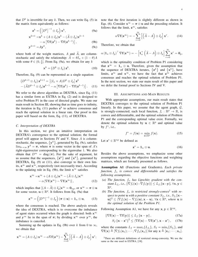
We consider the network topology as the digraph shown inFig. 1. We first apply the local degree weighting strategy, i.e.,to assign each agent itself and its out-neighbors equal weightsaccording to the agent’s own out-degree, i.e.,

aij =1

|N outj |

, (i, j) ∈ E . (54)

According to this strategy, the corresponding network parame-ters are shown in Fig. 1. We now estimate the interval of appro-priate step-sizes. We choose Lf = maxi{2λmax(H>i Hi)} =0.14, and Sf = mini{2λmin(H>i Hi)} = 0.1. We set η =0.04 < Sf/d

2, and δ = 0.1. Note that η and δ are estimatedvalues. According to the calculation, we have C1 = 36.6 and

C2 = 5.6. Therefore, we estimate that α =ηλmin(M+M>)

2L2f (d−∞d−)2

=

0.26, and α <Sf/(2d

2)−η/22C2δ

= 9.6 × 10−4. We thus pickα = 0.1 ∈ [α, α] for the following experiments.

23 1

56 47

10 89

Fig. 1: Strongly-connected but non-balanced digraphs and network parameters.

Our first experiment compares several algorithms suitedto directed graphs, illustrated in Fig. 1. The comparison ofDEXTRA, GP, D-DGD and DGD with weighting matrix beingrow-stochastic is shown in Fig. 2. In this experiment, weset α = 0.1, which is in the range of our theoretical valuecalculated above. The convergence rate of DEXTRA is linearas stated in Section III. G-P and D-DGD apply the same step-size, α = α√

k. As a result, the convergence rate of both is

sub-linear. We also consider the DGD algorithm, but with theweighting matrix being row-stochastic. The reason is that in adirected graph, it is impossible to construct a doubly-stochasticmatrix. As expected, DGD with row-stochastic matrix doesnot converge to the exact optimal solution while other threealgorithms are suited to directed graphs.

0 500 1000 1500 200010

−10

10−8

10−6

10−4

10−2

100

k

Residual

DGD with Row−Stochastic MatrixGPD−DGDDEXTRA

Fig. 2: Comparison of different distributed optimization algorithms in a leastsquares problem. GP, D-DGD, and DEXTRA are proved to work when thenetwork topology is described by digraphs. Moreover, DEXTRA has a linearconvergence rate compared with GP and D-DGD.

According to the theoretical value of α and α, we are able toset available step-size, α ∈ [9.6×10−4, 0.26]. In practice, this

10

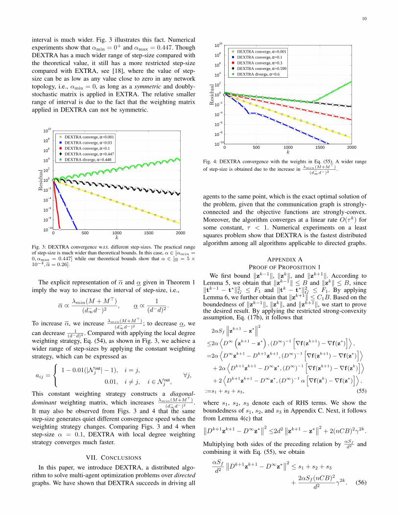
interval is much wider. Fig. 3 illustrates this fact. Numericalexperiments show that αmin = 0+ and αmax = 0.447. ThoughDEXTRA has a much wider range of step-size compared withthe theoretical value, it still has a more restricted step-sizecompared with EXTRA, see [18], where the value of step-size can be as low as any value close to zero in any networktopology, i.e., αmin = 0, as long as a symmetric and doubly-stochastic matrix is applied in EXTRA. The relative smallerrange of interval is due to the fact that the weighting matrixapplied in DEXTRA can not be symmetric.

0 500 1000 1500 200010

−10

10−8

10−6

10−4

10−2

100

102

104

106

108

1010

k

Residual

DEXTRA converge, α=0.001DEXTRA converge, α=0.03DEXTRA converge, α=0.1DEXTRA converge, α=0.447DEXTRA diverge, α=0.448

Fig. 3: DEXTRA convergence w.r.t. different step-sizes. The practical rangeof step-size is much wider than theoretical bounds. In this case, α ∈ [αmin =0, αmax = 0.447] while our theoretical bounds show that α ∈ [α = 5 ×10−4, α = 0.26].

The explicit representation of α and α given in Theorem 1imply the way to increase the interval of step-size, i.e.,

α ∝λmin(M +M>)

(d−∞d−)2, α ∝

1

(d−d)2.

To increase α, we increase λmin(M+M>)

(d−∞d−)2; to decrease α, we

can decrease 1(d−d)2 . Compared with applying the local degree

weighting strategy, Eq. (54), as shown in Fig. 3, we achieve awider range of step-sizes by applying the constant weightingstrategy, which can be expressed as

aij =

1− 0.01(|N outj | − 1), i = j,

0.01, i 6= j, i ∈ N outj ,

∀j,

This constant weighting strategy constructs a diagonal-dominant weighting matrix, which increases λmin(M+M>)

(d−∞d−)2.

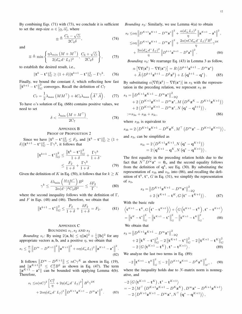
It may also be observed from Figs. 3 and 4 that the samestep-size generates quiet different convergence speed when theweighting strategy changes. Comparing Figs. 3 and 4 whenstep-size α = 0.1, DEXTRA with local degree weightingstrategy converges much faster.

VII. CONCLUSIONS

In this paper, we introduce DEXTRA, a distributed algo-rithm to solve multi-agent optimization problems over directedgraphs. We have shown that DEXTRA succeeds in driving all

0 500 1000 1500 200010

−10

10−8

10−6

10−4

10−2

100

102

104

106

108

1010

k

Residual

DEXTRA converge, α=0.001DEXTRA converge, α=0.1DEXTRA converge, α=0.3DEXTRA converge, α=0.599DEXTRA diverge, α=0.6

Fig. 4: DEXTRA convergence with the weights in Eq. (55). A wider rangeof step-size is obtained due to the increase in λmin(M+M>)

(d−∞d−)2.

agents to the same point, which is the exact optimal solution ofthe problem, given that the communication graph is strongly-connected and the objective functions are strongly-convex.Moreover, the algorithm converges at a linear rate O(τk) forsome constant, τ < 1. Numerical experiments on a leastsquares problem show that DEXTRA is the fastest distributedalgorithm among all algorithms applicable to directed graphs.

APPENDIX APROOF OF PROPOSITION 1

We first bound ‖zk−1‖, ‖zk‖, and ‖zk+1‖. According toLemma 5, we obtain that ‖zk−1‖ ≤ B and ‖zk‖ ≤ B, since‖tk−1 − t∗‖2G ≤ F1 and ‖tk − t∗‖2G ≤ F1. By applyingLemma 6, we further obtain that ‖zk+1‖ ≤ C1B. Based on theboundedness of ‖zk−1‖, ‖zk‖, and ‖zk+1‖, we start to provethe desired result. By applying the restricted strong-convexityassumption, Eq. (17b), it follows that

2αSf

∥∥∥zk+1 − z∗∥∥∥2

≤2α⟨D∞

(zk+1 − z∗

), (D∞)−1

[∇f(zk+1)−∇f(z∗)

]⟩,

=2α⟨D∞zk+1 −Dk+1zk+1, (D∞)−1

[∇f(zk+1)−∇f(z∗)

]⟩+ 2α

⟨Dk+1zk+1 −D∞z∗, (D∞)−1

[∇f(zk+1)−∇f(zk)

]⟩+ 2

⟨Dk+1zk+1 −D∞z∗, (D∞)−1 α

[∇f(zk)−∇f(z∗)

]⟩,

:=s1 + s2 + s3, (55)

where s1, s2, s3 denote each of RHS terms. We show theboundedness of s1, s2, and s3 in Appendix C. Next, it followsfrom Lemma 4(c) that∥∥Dk+1zk+1 −D∞z∗

∥∥2 ≤2d2∥∥zk+1 − z∗

∥∥2+ 2(nCB)2γ2k.

Multiplying both sides of the preceding relation by αSfd2 and

combining it with Eq. (55), we obtain

αSfd2

∥∥Dk+1zk+1 −D∞z∗∥∥2 ≤ s1 + s2 + s3

+2αSf (nCB)2

d2γ2k. (56)

11

By plugging the related bounds from Appendix C (s1 fromEq. (83), s2 from Eq. (84), and s3 from Eq. (92)) in Eq. (56),it follows that∥∥tk − t∗

∥∥2

G−∥∥tk+1 − t∗

∥∥2

G

≥∥∥Dk+1zk+1 −D∞z∗

∥∥2α2

[Sf

d2−η−2η(d−∞d−Lf )2

]In− 1

δ In+Q

+∥∥Dk+1zk+1 −Dkzk

∥∥2

M>− δ2MM>−α(d−∞d−Lf )2

η In

− α(nC)2

[C2

1

2η+ (d−∞d

−Lf )2

(η +

1

η

)+Sfd2

]B2γk

−∥∥q∗ − qk+1

∥∥2δ2NN

> . (57)

In order to derive the relation that∥∥tk − t∗∥∥2

G≥ (1 + δ)

∥∥tk+1 − t∗∥∥2

G− Γγk, (58)

it is sufficient to show that the RHS of Eq. (57) is no less thanδ∥∥tk+1 − t∗

∥∥2

G−Γγk. Recall the definition of G, tk, and t∗

in Eq. (31), we have

δ∥∥tk+1 − t∗

∥∥2

G− Γγk =

∥∥Dk+1zk+1 −D∞z∗∥∥2

δM>

+∥∥q∗ − qk+1

∥∥2

δN− Γγk. (59)

Comparing Eqs. (57) with (59), it is sufficient to prove that∥∥Dk+1zk+1 −D∞z∗∥∥2α2

[Sf

d2−η−2η(d−∞d−Lf )2

]In− 1

δ In+Q−δM>

+∥∥Dk+1zk+1 −Dkzk

∥∥2

M>− δ2MM>−α(d−∞d−Lf )2

η In

+ Γγk − α(nC)2

[C2

1

2η+ (d−∞d

−Lf )2

(η +

1

η

)+Sfd2

]B2γk

≥∥∥q∗ − qk+1

∥∥2

δ(NN>

2 +N) . (60)

We next aim to bound ‖q∗ − qk+1‖2δ(NN

>2 +N)

in terms of

‖Dk+1zk+1−D∞z∗‖ and ‖Dk+1zk+1−Dkzk‖, such that itis easier to analyze Eq. (60). From Lemma 3, we have∥∥q∗ − qk+1

∥∥2

L>L

=∥∥L (q∗ − qk+1

)∥∥2,

=∥∥∥R(Dk+1zk+1 −D∞z∗) + α[∇f(zk+1)−∇f(z∗)]

+ A(Dk+1zk+1 −Dkzk) + α[∇f(zk)−∇f(zk+1)]∥∥∥2

,

≤4(∥∥Dk+1zk+1 −D∞z∗

∥∥2

R>R+ α2L2

f

∥∥zk+1 − z∗∥∥2)

+ 4(∥∥Dk+1zk+1 −Dkzk

∥∥2

A>A+ α2L2

f

∥∥zk+1 − zk∥∥2),

≤∥∥Dk+1zk+1 −D∞z∗

∥∥2

4R>R+8(αLfd−)2In

+∥∥Dk+1zk+1 −Dkzk

∥∥2

4A>A+8(αLfd−)2In

+ 24(αnCd−Lf

)2B2γk. (61)

Since that λ(N+N>

2

)≥ 0, λ

(NN>

)≥ 0, λ

(L>L

)≥ 0,

and λmin

(N+N>

2

)= λmin

(NN>

)= λmin

(L>L

)= 0 with

the same corresponding eigenvector, we have∥∥q∗ − qk+1∥∥2

δ(NN>

2 +N) ≤ δC2

∥∥q∗ − qk+1∥∥2

L>L, (62)

where C2 is the constant defined in Theorem 1. By combiningEqs. (61) with (62), it follows that∥∥q∗ − qk+1

∥∥2

δ(NN>

2 +N) ≤ δC2

∥∥q∗ − qk+1∥∥2

L>L,

≤∥∥Dk+1zk+1 −D∞z∗

∥∥2

δC2(4R>R+8(αLfd−)2In)

+∥∥Dk+1zk+1 −Dkzk

∥∥2

δC2(4A>A+8(αLfd−)2In)

+ 24δC2

(αnCd−Lf

)2B2γk. (63)

Consider Eq. (60), together with (63). Let

Γ =C3B2, (64)

where C3 is the constant defined in Theorem 1, such thatall “γk items” in Eqs. (60) and (63) can be canceled out. Inorder to prove Eq. (60), it is sufficient to show that the LHSof Eq. (60) is no less than the RHS of Eq. (63), i.e.,∥∥Dk+1zk+1 −D∞z∗

∥∥2α2

[Sf

d2−η−2η(d−∞d−Lf )2

]In− 1

δ In+Q−δM>

+∥∥Dk+1zk+1 −Dkzk

∥∥2

M>− δ2MM>−α(d−∞d−Lf )2

η In

≥∥∥Dk+1zk+1 −D∞z∗

∥∥2

δC2(4R>R+8(αLfd−)2In)

+∥∥Dk+1zk+1 −Dkszk

∥∥2

δC2(4A>A+8(αLfd−)2In) . (65)

To satisfy Eq. (65), it is sufficient to have the following tworelations hold simultaneously,

α

2

[Sfd2− η − 2η(d−∞d

−Lf )2

]− 1

δ− δλmax

(M +M>

2

)≥δC2

[4λmax

(R>R

)+ 8(αLfd

−)2], (66a)

λmin

(M +M>

2

)− δ

2λmax

(MM>

)− α(d−∞d

−Lf )2

η

≥δC2

[4λmax

(A>A

)+ 8(αLfd

−)2]. (66b)

where in Eq. (66a) we ignore the termλmin(Q+Q>)

2 due toλmin

(Q+Q>

)= 0. Recall the definition

C4 = 8C2

(Lfd

−)2 , (67)

C5 = λmax

(M +M>

2

)+ 4C2λmax

(R>R

), (68)

C6 =Sfd2 − η − 2η(d−∞d

−Lf )2

2, (69)

∆ = C26 − 4C4δ

(1

δ+ C5δ

). (70)

The solution of step-size, α, satisfying Eq. (66a), is

C6 −√

∆

2C4δ≤ α ≤ C6 +

√∆

2C4δ, (71)

where we set

η <Sf

d2(1 + (d−∞d−Lf )2), (72)

to ensure the solution of α contains positive values. In orderto have δ > 0 in Eq. (66b), the step-size, α, is sufficient tosatisfy

α ≤ηλmin

(M +M>

)2(d−∞d−Lf )2

. (73)

12

By combining Eqs. (71) with (73), we conclude it is sufficientto set the step-size α ∈ [α, α], where

α ,C6 −

√4

2C4δ, (74)

and

α , min

{ηλmin

(M +M>

)2(d−∞d−Lf )2

,C6 +

√4

2C4δ

}, (75)

to establish the desired result, i.e.,

‖tk − t∗‖2G ≥ (1 + δ)‖tk+1 − t∗‖2G − Γγk. (76)

Finally, we bound the constant δ, which reflecting how fast∥∥tk+1 − t∗∥∥2

Gconverges. Recall the definition of C7

C7 =1

2λmax

(MM>

)+ 4C2λmax

(A>A

). (77)

To have α’s solution of Eq. (66b) contains positive values, weneed to set

δ <λmin

(M +M>

)2C7

. (78)

APPENDIX BPROOF OF PROPOSITION 2

Since we have ‖tk − t∗‖2G ≤ F2, and ‖tk − t∗‖2G ≥ (1 +δ)‖tk+1 − t∗‖2G − Γγk, it follows that

∥∥tk+1 − t∗∥∥2

G≤∥∥tk − t∗

∥∥2

G

1 + δ+

Γγk

1 + δ,

≤ F2

1 + δ+

Γγk

1 + δ. (79)

Given the definition of K in Eq. (50), it follows that for k ≥ K

γk ≤δλmin

(M+M>

2

)B2

2α(d−)2C3B2≤ δF2

Γ, (80)

where the second inequality follows with the definition of Γ,and F in Eqs. (48) and (46). Therefore, we obtain that∥∥tk+1 − t∗

∥∥2

G≤ F2

1 + δ+

δF2

1 + δ= F2. (81)

APPENDIX CBOUNDING s1, s2 AND s3

Bounding s1: By using 2〈a,b〉 ≤ η‖a‖2 + 1η‖b‖

2 for anyappropriate vectors a,b, and a positive η, we obtain that

s1 ≤α

η

∥∥∥D∞ −DK+1∥∥∥2 ∥∥∥zK+1

∥∥∥2 + αη(d−∞Lf )2∥∥∥zK+1 − z∗

∥∥∥2 .(82)

It follows∥∥D∞ −DK+1

∥∥ ≤ nCγK as shown in Eq. (19),and ‖zK+1‖2 ≤ C2

1B2 as shown in Eq. (47). The term

‖zK+1 − z∗‖ can be bounded with applying Lemma 4(b).Therefore,

s1 ≤α(nC)2[C2

1

η+ 2η(d−∞d

−Lf )2

]B2γ2K

+ 2αη(d−∞d−Lf )

2∥∥∥DK+1zK+1 −D∞z∗

∥∥∥2 . (83)

Bounding s2: Similarly, we use Lemma 4(a) to obtain

s2 ≤αη∥∥∥DK+1zK+1 −D∞z∗

∥∥∥2 + α(d−∞Lf )2

η

∥∥∥zK+1 − zk∥∥∥2 ,

≤αη∥∥∥DK+1zK+1 −D∞z∗

∥∥∥2 + 2α(nCd−∞d−Lf )

2B2

ηγ2K

+2α(d−∞d

−Lf )2

η

∥∥∥Dk+1zk+1 −Dkzk∥∥∥2 . (84)

Bounding s3: We rearrange Eq. (43) in Lemma 3 as follow,

α[∇f(zk)−∇f(z∗)

]= R

(Dk+1zk+1 −D∞z∗

)+ A

(Dk+1zk+1 −Dkzk

)+ L

(qk+1 − q∗

). (85)

By substituting α[∇f(zk)−∇f(z∗)] in s3 with the represen-tation in the preceding relation, we represent s3 as

s3 =∥∥DK+1zK+1 −D∞z∗

∥∥2

−2Q

+ 2⟨DK+1zK+1 −D∞z∗,M

(DKzK −DK+1zK+1

)⟩+ 2

⟨DK+1zK+1 −D∞z∗, N

(q∗ − qk+1

)⟩,

:=s3a + s3b + s3c, (86)

where s3b is equivalent to

s3b = 2⟨DK+1zK+1 −DKzK ,M>

(D∞z∗ −DK+1zK+1

)⟩,

and s3c can be simplified as

s3c = 2⟨DK+1zK+1, N

(q∗ − qK+1

)⟩= 2

⟨qK+1 − qK , N

(q∗ − qK+1

)⟩.

The first equality in the preceding relation holds due to thefact that N>D∞z∗ = 0n and the second equality followsfrom the definition of qk, see Eq. (30). By substituting therepresentation of s3b and s3c into (86), and recalling the defi-nition of tk, t∗, G in Eq. (31), we simplify the representationof s3,

s3 =∥∥DK+1zK+1 −D∞z∗

∥∥2

−2Q

+ 2⟨tK+1 − tK , G

(t∗ − tK+1

)⟩. (87)

With the basic rule⟨tK+1 − tK , G

(t∗ − tK+1

)⟩+⟨G(tK+1 − tK

), t∗ − tK+1

⟩=∥∥∥tK − t∗

∥∥∥2G−∥∥∥tK+1 − t∗

∥∥∥2G−∥∥∥tK+1 − tK

∥∥∥2G, (88)

We obtain that

s3 =∥∥DK+1zK+1 −D∞z∗

∥∥2

−2Q

+ 2∥∥tK − t∗

∥∥2

G− 2

∥∥tK+1 − t∗∥∥2

G− 2

∥∥tK+1 − tK∥∥2

G

− 2⟨G(tK+1 − tK

), t∗ − tK+1

⟩. (89)

We analyze the last two terms in Eq. (89):

−2∥∥∥tK+1 − tK

∥∥∥2G≤− 2

∥∥∥DK+1zK+1 −DKzK∥∥∥2M>

, (90)

where the inequality holds due to N -matrix norm is nonneg-ative, and

−2⟨G(tK+1 − tK

), t∗ − tK+1

⟩=− 2

⟨M>

(DK+1zK+1 −DKzK

), D∞z∗ −DK+1zK+1

⟩− 2

⟨DK+1zK+1 −D∞z∗, N>

(q∗ − qK+1

)⟩,

13

≤δ∥∥DK+1zK+1 −DKzK

∥∥2

MM>+ δ

∥∥q∗ − qK+1∥∥2

NN>

+2

δ

∥∥DK+1zK+1 −D∞z∗∥∥2, (91)

for some δ > 0. By substituting Eqs. (90) and (91) intoEq. (89), we obtain that

s3 ≤2∥∥tK − t∗

∥∥2

G− 2

∥∥tK+1 − t∗∥∥2

G+∥∥q∗ − qK+1

∥∥2

δNN>

+∥∥DK+1zK+1 −D∞z∗

∥∥22δ In−2Q

+∥∥DK+1zK+1 −DKzK

∥∥2

−2M>+δMM>. (92)

REFERENCES[1] V. Cevher, S. Becker, and M. Schmidt, “Convex optimization for

big data: Scalable, randomized, and parallel algorithms for big dataanalytics,” IEEE Signal Processing Magazine, vol. 31, no. 5, pp. 32–43,2014.

[2] S. Boyd, N. Parikh, E. Chu, B. Peleato, and J. Eckstein, “Distributedoptimization and statistical learning via the alternating direction methodof multipliers,” Foundation and Trends in Maching Learning, vol. 3, no.1, pp. 1–122, Jan. 2011.

[3] I. Necoara and J. A. K. Suykens, “Application of a smoothing techniqueto decomposition in convex optimization,” IEEE Transactions onAutomatic Control, vol. 53, no. 11, pp. 2674–2679, Dec. 2008.

[4] G. Mateos, J. A. Bazerque, and G. B. Giannakis, “Distributed sparselinear regression,” IEEE Transactions on Signal Processing, vol. 58, no.10, pp. 5262–5276, Oct. 2010.

[5] J. A. Bazerque and G. B. Giannakis, “Distributed spectrum sensing forcognitive radio networks by exploiting sparsity,” IEEE Transactions onSignal Processing, vol. 58, no. 3, pp. 1847–1862, March 2010.

[6] M. Rabbat and R. Nowak, “Distributed optimization in sensor networks,”in 3rd International Symposium on Information Processing in SensorNetworks, Berkeley, CA, Apr. 2004, pp. 20–27.

[7] U. A. Khan, S. Kar, and J. M. F. Moura, “Diland: An algorithm fordistributed sensor localization with noisy distance measurements,” IEEETransactions on Signal Processing, vol. 58, no. 3, pp. 1940–1947, Mar.2010.

[8] C. L and L. Li, “A distributed multiple dimensional qos constrainedresource scheduling optimization policy in computational grid,” Journalof Computer and System Sciences, vol. 72, no. 4, pp. 706 – 726, 2006.

[9] G. Neglia, G. Reina, and S. Alouf, “Distributed gradient optimizationfor epidemic routing: A preliminary evaluation,” in 2nd IFIP in IEEEWireless Days, Paris, Dec. 2009, pp. 1–6.

[10] A. Nedic and A. Ozdaglar, “Distributed subgradient methods for multi-agent optimization,” IEEE Transactions on Automatic Control, vol. 54,no. 1, pp. 48–61, Jan. 2009.

[11] K. Yuan, Q. Ling, and W. Yin, “On the convergence of decentralizedgradient descent,” arXiv preprint arXiv:1310.7063, 2013.

[12] J. C. Duchi, A. Agarwal, and M. J. Wainwright, “Dual averaging fordistributed optimization: Convergence analysis and network scaling,”IEEE Transactions on Automatic Control, vol. 57, no. 3, pp. 592–606,Mar. 2012.

[13] J. F. C. Mota, J. M. F. Xavier, P. M. Q. Aguiar, and M. Puschel, “D-ADMM: A communication-efficient distributed algorithm for separableoptimization,” IEEE Transactions on Signal Processing, vol. 61, no. 10,pp. 2718–2723, May 2013.

[14] E. Wei and A. Ozdaglar, “Distributed alternating direction method ofmultipliers,” in 51st IEEE Annual Conference on Decision and Control,Dec. 2012, pp. 5445–5450.

[15] W. Shi, Q. Ling, K Yuan, G Wu, and W Yin, “On the linearconvergence of the admm in decentralized consensus optimization,”IEEE Transactions on Signal Processing, vol. 62, no. 7, pp. 1750–1761,April 2014.

[16] D. Jakovetic, J. Xavier, and J. M. F. Moura, “Fast distributed gradientmethods,” IEEE Transactions on Automatic Control, vol. 59, no. 5, pp.1131–1146, 2014.

[17] Q. Ling and A. Ribeiro, “Decentralized linearized alternating directionmethod of multipliers,” in IEEE International Conference on Acoustics,Speech and Signal Processing. IEEE, 2014, pp. 5447–5451.

[18] W. Shi, Q. Ling, G. Wu, and W Yin, “Extra: An exact first-orderalgorithm for decentralized consensus optimization,” SIAM Journal onOptimization, vol. 25, no. 2, pp. 944–966, 2015.

[19] A. Mokhatari, Q. Ling, and A. Ribeiro, “Network newton,” http://www.seas.upenn.edu/∼aryanm/wiki/NN.pdf, 2014.

[20] A. Nedic and A. Olshevsky, “Distributed optimization over time-varyingdirected graphs,” IEEE Transactions on Automatic Control, vol. PP, no.99, pp. 1–1, 2014.

[21] K. I. Tsianos, S. Lawlor, and M. G. Rabbat, “Push-sum distributed dualaveraging for convex optimization,” in 51st IEEE Annual Conferenceon Decision and Control, Maui, Hawaii, Dec. 2012, pp. 5453–5458.

[22] K. I. Tsianos, The role of the Network in Distributed Optimization Al-gorithms: Convergence Rates, Scalability, Communication/ComputationTradeoffs and Communication Delays, Ph.D. thesis, Dept. Elect. Comp.Eng. McGill University, 2013.

[23] K. I. Tsianos, S. Lawlor, and M. G. Rabbat, “Consensus-baseddistributed optimization: Practical issues and applications in large-scalemachine learning,” in 50th Annual Allerton Conference on Communi-cation, Control, and Computing, Monticello, IL, USA, Oct. 2012, pp.1543–1550.

[24] D. Kempe, A. Dobra, and J. Gehrke, “Gossip-based computation of ag-gregate information,” in 44th Annual IEEE Symposium on Foundationsof Computer Science, Oct. 2003, pp. 482–491.

[25] F. Benezit, V. Blondel, P. Thiran, J. Tsitsiklis, and M. Vetterli, “Weightedgossip: Distributed averaging using non-doubly stochastic matrices,” inIEEE International Symposium on Information Theory, Jun. 2010, pp.1753–1757.

[26] A. Jadbabaie, J. Lim, and A. S. Morse, “Coordination of groupsof mobile autonomous agents using nearest neighbor rules,” IEEETransactions on Automatic Control, vol. 48, no. 6, pp. 988–1001, Jun.2003.

[27] R. Olfati-Saber and R. M. Murray, “Consensus problems in networksof agents with switching topology and time-delays,” IEEE Transactionson Automatic Control, vol. 49, no. 9, pp. 1520–1533, Sep. 2004.

[28] R. Olfati-Saber and R. M. Murray, “Consensus protocols for networksof dynamic agents,” in IEEE American Control Conference, Denver,Colorado, Jun. 2003, vol. 2, pp. 951–956.

[29] L. Xiao, S. Boyd, and S. J. Kim, “Distributed average consensuswith least-mean-square deviation,” Journal of Parallel and DistributedComputing, vol. 67, no. 1, pp. 33 – 46, 2007.

[30] C. Xi, Q. Wu, and U. A. Khan, “Distributed gradient descent overdirected graphs,” arXiv preprint arXiv:1510.02146, 2015.

[31] C. Xi and U. A. Khan, “Distributed subgradient projection algorithmover directed graphs,” arXiv preprint arXiv:1602.00653, 2016.

[32] K. Cai and H. Ishii, “Average consensus on general strongly connecteddigraphs,” Automatica, vol. 48, no. 11, pp. 2750 – 2761, 2012.

[33] A. Makhdoumi and A. Ozdaglar, “Graph balancing for distributedsubgradient methods over directed graphs,” to appear in 54th IEEEAnnual Conference on Decision and Control, 2015.

[34] L. Hooi-Tong, “On a class of directed graphswith an application totraffic-flow problems,” Operations Research, vol. 18, no. 1, pp. 87–94,1970.

[35] A. Nedic and A. Olshevsky, “Distributed optimization of strongly convexfunctions on directed time-varying graphs,” in IEEE Global Conferenceon Signal and Information Processing, Dec. 2013, pp. 329–332.

[36] C. Xi and U. A. Khan, “On the linear convergence of distributedoptimization over directed graphs,” arXiv preprint arXiv:1510.02149,2015.

[37] J. Zeng and W. Yin, “Extrapush for convex smooth decentralizedoptimization over directed networks,” arXiv preprint arXiv:1511.02942,2015.

[38] G. W. Stewart, “Matrix perturbation theory,” 1990.[39] R. Bhatia, Matrix analysis, vol. 169, Springer Science & Business

Media, 2013.[40] F. Chung, “Laplacians and the cheeger inequality for directed graphs,”

Annals of Combinatorics, vol. 9, no. 1, pp. 1–19, 2005.