On the Impact of Real-Time Information...

1

On the Impact of Real-Time Information on

Field Service Scheduling

Ioannis Petrakis, Christian Hass, Martin Bichler 1

Department of Informatics, TU München, Germany

Mobile phone operators need to plan and schedule field force personnel for maintenance and repair

tasks on mobile phone base stations across the country on a daily basis. In this paper, we will

introduce the field force scheduling problem with priorities. Motivated by the rising popularity of

mobile field force management solutions, we compare online and offline heuristics as well as hybrids

to solve the problem. The results help understand the benefits of dynamic scheduling based on real-

time position information as compared to traditional daily offline planning.

Keywords: Routing ; Heuristics; Real-time

1 Introduction

Arguably, one of the most important planning problems in many large service organizations is the

allocation of employees to tasks. This problem comes in many variants, such as project scheduling,

staff scheduling, and rostering [18], [9], [42]. The assignment of the field workforce to tasks that are

spatially distributed is different, because the planner needs to take into account travel times and

routing constraints.

In this paper, we will focus on a particular task assignment problem, which arises when the mobile

workforce has to accomplish spatially distributed tasks with different priorities, deadlines, and skill

requirements. As a real-world example, we will use the daily planning problem of a European mobile

phone provider. The operator has almost 20,000 mobile phone base stations, which require

maintenance and irregular upgrades or need to be repaired immediately in the event of a failure.

Several hundred engineers carry out these tasks. Each day, the engineers start at their home location,

1 Contact author: Ioannis Petrakis, Department of Informatics, TU München, Boltzmannstr. 3, 85748 Garching, Tel.: +49-89-289-17530, Fax: +49-89-289-17535, [email protected]

2

complete around three to five tasks, and return to their home. Each task requires a specific skill, and

each engineer possesses a number of skills. Tasks also have deadlines and priorities, which depend on

the nature of the task (e.g., service-affecting disturbances have high priority compared to regular

maintenance). Every morning the scheduler assigns tasks to field engineers and suggests a route for

the day, which may be later modified. We will refer to this problem as field service scheduling with

priorities (FSSP).

The planning problem has similarities with different types of vehicle routing problems (VRP), such as

the Multi-Depot Vehicle Routing Problem (MDVRP) ([4]) or the Pickup and Delivery Problem (PDP)

[39]. These problems are NP-hard and can only be solved exactly for rather small instances, as has

been shown in experimental analyses ([23],[24],[1]). The FSSP has a number of notable differences to

the MDVRP. For example, in each depot only one vehicle (engineer) is located; the same vehicle must

be routed each day, resulting in exactly one route for each vehicle and day; the customers (tasks)

require skills and have deadlines and associated penalties for violating these deadlines; there are no

truck load capacities for each vehicle, but service and travel times as well as hard overtime limits need

to be considered instead. Some of these differences have a profound impact on the design of specific

algorithms to solve the problem.

Priorities and deadlines do not only influence the design of an offline algorithm for the planning stage

each morning. Urgent tasks arising during the day need to be allocated to a field engineer as soon as

possible, which causes deviations from the planned schedule. Overall, the computational complexity

of the planning problem and the stochastic nature of travel times and service times for individual tasks

remains a challenge for respective optimization and decision support systems in industry.

IT solutions have significantly changed field service scheduling. Mobile devices and GPS lead to real-

time data about the location of field force engineers. Having a mobile solution integrated with

automated task assignment enables dynamic route scheduling throughout the day, as engineers can be

reassigned or rerouted. Software for field service management, also referred to as mobile workforce

optimization, combines mobile technology with dynamic scheduling and assignment of tasks [29].

Apart from the manual allocation of tasks to mobile engineers, respective software typically provides

3

rule-based heuristics to automatically route engineers and schedule their tasks. Unfortunately, little is

published on dispatching rules and algorithms used for respective dynamic scheduling solutions. In

most combinatorial optimization problems, dynamic aspects are not very well studied [39]. However,

there have been a number of proposals in the academic literature to handle dynamism in traditional

VRPs, ranging from simple assignment rules to solving the planning problem repeatedly (see Section

2).

In this work, we suggest and analyze static (offline) and dynamic (online) algorithms to solve the

FSSP. Offline algorithms generate static routes once a day in the morning, whereas online algorithms

can process new tasks arriving throughout the day immediately and update routing schedules in real

time. Some of these heuristics are adapted from successful algorithmic approaches to related VRPs.

While different algorithmic approaches will lead to different results, the analysis will provide a better

understanding of the benefits of mobile field service management solutions with dynamic scheduling.

From a managerial point of view, this should provide evidence whether the introduction of dynamic

scheduling solutions lead to significant cost savings or not. The experimental analysis is based on real-

world data of a European mobile phone provider, but we conjecture that the situation is representative

for other mobile phone providers or other industries with distributed repair and maintenance tasks such

as in the utilities industries. The degree of dynamism, i.e., the frequency with which new tasks arrive

throughout the day, will be a treatment variable in the experiments.

We will first provide a succinct formal problem description of this planning problem in the

telecommunication industry. Unfortunately, standard branch-and-cut approaches can only solve very

small instances of the problem, as is the case for most large VRPs. Therefore, we will suggest

heuristics for the FSSP that can be used to solve the problem statically every morning or dynamically

throughout the day, if the tasks are not known a priori. Several heuristics are based on those which

have recently been applied successfully for related VRPs. Finally, we will provide the results of an

experimental evaluation based on real-world data, in which we compare static, dynamic, and hybrid

scheduling approaches, allowing us to evaluate the relative efficiency of these approaches. While there

are differences among different algorithmic approaches, the main differences stem from the

4

availability of real-time information throughout the day. We will further analyze the robustness of our

results and of the different heuristics with respect to different treatments, such as different proportions

of urgent tasks or arrival rates.

In contrast to existing literature in vehicle routing, our primary goal is not to develop new algorithmic

approaches to solving the problem, but to get an understanding of the efficiency gains of dynamic

scheduling made possible by real-time availability of location information about field force engineers

as compared to static scheduling at fixed time intervals without such information available. While

different scheduling algorithms will lead to somewhat different results, we conjecture that the

differences between static and dynamic scheduling will be on the same order of magnitude in similar

applications.

The managerial impact of dynamic or static scheduling is substantial. Already in our base scenario the

total costs (travel times and deadline penalties) were 2.68 times higher than the costs of the online

heuristic. In contrast, for the hybrid heuristic, which imitates a human dispatcher scheduling manually

throughout the day, costs were 44% higher than those of the online heuristic in the base scenario.

These numbers can change depending on the number of new tasks arriving every day, the number of

engineers, and the deadline penalties, which is why we describe a number of different scenarios in our

experimental evaluation. Nevertheless, given that the operation of field force personnel causes costs in

the order of millions of dollars annually for any telecom operator, this decision has significant

managerial impact. We show that the savings in operational costs through online scheduling can be

substantial, when compared with a pure offline planning solution. A skilled human dispatcher can

reduce this cost difference significantly, however.

2 Related Literature

The FSSP is related to the class of vehicle routing problems (VRP) [7]. A number of variants have

been developed over time. In the Multi-Depot Vehicle Routing Problem (MDVRP) a company has

several depots from which it may serve customers. The objective is to minimize the vehicle fleet and

the sum of travel times. The total demand for commodities has to be served from several depots. The

MDVRP, in particular the version with time windows, has a number of similarities to the FSSP, where

5

the depots are the home locations of engineers and the customers are the tasks in the mobile base

stations.

2.1 Multi-Depot VRPs

There are a number of computational results on the MDVRP often based on benchmark problems [17].

For example, exact solutions have been proposed by [1]. Only instances with 200 customers and five

depots could be solved within six hours. Many different heuristic approaches and metaheuristics have

been used for the MDVRP, but a detailed review of the different approaches would be beyond the

scope of this article. It should be noted, however, that tabu search algorithms are responsible for many

good solutions of the benchmark instances mentioned above [4]. More recently, [32] suggested a

rather general heuristic for different types of VRPs. These types of VRPs are transformed into a

general model and solved using the adaptive large neighborhood search method [37], [38].

MDVRPTW is an extension of the MDVRP which allows for time windows. There has been much

less research on this problem compared to the general MDVRP. Tabu search has also led to good

results for the MDVRPTW [5]. A number of recent advances have been made based on variable

neighborhood search heuristics [34], [33].

While there are similarities, there are also a number of differences between FSSP and the

MDVRPTW. In MDVRPTW all customers need to be visited and the objective is to minimize the

vehicle fleet and travel time. In FSSP, an engineer tries to visit as many tasks as possible (weighted by

priority) on the same day with a given fixed number of engineers. All tasks that could not be

completed on the same day will be rescheduled with new tasks the next day. In the MDVRPTW the

time windows (TW) are binding as they typically correspond to opening hours or time slots agreed

with the customer. A schedule visiting a customer outside a time window is infeasible. In FSSP there

are no fixed time windows for visiting a base station, but there are penalties for being late. This is

sometimes referred to as “soft time windows” in VRPTWs. In MDVRPTW the vehicles may have to

wait at the customer’s location for the start of the time window. This cannot occur in FSSP as the tasks

can be accomplished as soon as they arise and are reported. Other differences are that in FSSP there is

only a single vehicle in each depot or home location and there are no load constraints on the vehicle.

6

In contrast, skill sets of different drivers (engineers) need to be considered. Finally, one needs to

consider service times for different tasks, which is not always an issue in VRPs. For the design of

heuristics these differences matter.

2.2 Dynamic VRPs

The dynamic version of the FSSP is a main concern of this paper. Most of the existing VRP research

has been focused on problems of a deterministic and static nature. The increasing role of real-time

information on traffic network conditions have all led to a rise in the number of freight and fleet

management systems that are operating under dynamic conditions. In dynamic and stochastic routing

models, decisions must be made before all information needed is known. Some of the models deal

with a priori optimization in which a solution is generated for stochastic problems prior to the receipt

of information regarding the realization of its random elements. The general approach is to generate an

a priori solution that has the least cost in an expected sense. Other approaches involve making

decisions and observing outcomes on a continuous, rolling horizon. [11] report that very few cases of

commercial routing software with dynamic routing are known and most are focused on the design of

static routes. Designing a real-time routing algorithm depends to a large extent on the degree of

dynamism of the problem as defined by [28].

There has been some work on dynamic versions of the VRPs (DVRP) [25] with and without the

consideration of time windows but not specifically on the dynamic MDVRP. Algorithms can be

broadly divided into simple policies or rules, insertion procedures, and metaheuristics. [25] evaluate

simple policies such as First Come First Serve or Nearest Neighbor policies based on [2] in a dynamic

or partially dynamic setting. Insertion procedures insert new tasks in the best position of the current

routes on the basis of a rolling horizon [36] or double horizon [31]. More recent work is based on

metaheuristics, where a sequence of static VRPs is solved [16]. A survey of different types of DVRPs

and solution concepts can be found in [12]. While the basic problem is different to the FSSP, some

approaches to addressing the dynamism can be applied here as well.

7

2.3 Field Workforce Scheduling by British Telecom and Commercial Off-the-Shelf Software

British Telecom (BT) has reported on a field workforce scheduling project [26],[27]. They had to

schedule 20,000 engineers and the rule-based scheduling applications from various vendors were not

able to address the scale and the complexity of the requirements. BT therefore developed a heuristic

based on constraint-based reasoning and simulated annealing. They reported a saving of $150 million

per annum on engineer, and controller, and other workforce-related costs, such as vehicles, equipment,

tools, training, and administration. Unfortunately, little has been published on the details of the

algorithms and the respective experimental results. Also, the BT problem focused on engineers with

customer interaction and therefore has a number of characteristics that are beyond the FSSP. For

example, some tasks needed to be completed within an agreed-upon time window, as access to

customer premises may be granted only to certain individuals at certain times. Furthermore, task

duration depended on the engineer’s experience and skills. Also, some tasks had to be sequenced in

time or had to be performed in parallel.

As indicated in the introduction, nowadays there are several commercial software packages focusing

on field service management [29], but little is known about the dispatching rules and algorithms used.

A notable exception is IBM/Ilog Dispatcher, which is based on constraint programming [19]. While

constraint programming is a powerful approach to generating many good feasible solutions, we aim

for a single “best” proposal every morning in the offline setting.

3 The Field Service Scheduling with Priorities Problem

The FSSP can be described as follows: A number of n spatially distributed tasks must be served

exactly once by one of m engineers. Engineers have one shift and accomplish one tour per day. They

start their tours from their particular home bases, visit locations to fulfill particular tasks, and return

back home. Each tour has a soft and a hard time limit. Soft time limits cause additional costs

(overtime), whereas hard time limits must not be broken. The assignment of a task to an engineer is

only possible if the engineer has a certain skill required by the task. Each task has a duration (service

time) and its service must begin prior to its due date (deadline), otherwise penalty costs are charged

8

(deadline penalties). The priority of a task is reflected by its “penalty factor”; hence the deadline

penalties of a task are calculated by the time of delay multiplied by its penalty factor.

The goal of the FSSP is to minimize the sum of the following three goals:

1. Transportation costs measured by the total travel time (in minutes),

2. Deadline penalties, measured by the sum over all delayed tasks’ deadline penalties (delay time

in minutes multiplied by the penalty factor),

3. Overtime costs, measured by the total overtime (in minutes).

All three goals have minutes as the unit of measure. The delay time of high-priority tasks is however

multiplied by a penalty factor greater than one to account for the fact that violation of these deadlines

is less preferable to the mobile phone provider compared to additional travel time. There is a large

body of literature on multi-objective optimization, and several ways how the objective function could

be designed. The objective function introduced below was designed according to practical

considerations.

We now formalize the Field Service Scheduling with Priorities (FSSP) as a mixed integer program in

order to provide a succinct formal description of the problem. Our problem formulation assumes full

information setting (i.e. the service times of the tasks and their report dates are known in advance).

Hence the solution represents the ex-post optimal solution. We consider a multigraph � = ��, ��,

where the vertex set is divided into two disjoint subsets � = ��, �. Set � = �0,1, . . − 1� represents

the locations of the engineers’ homes. The set of engineers coincides with the set � as each engineer

has his own home location. Set = �0,1, . . � − 1� represents the tasks’ locations. � denotes the set of

days. � = �(�, �)�,�� with �, � ∈ �, � ∈ �, � ∈ � and � ≠ � is the arc set and �� = �� the travel time

from � to �. We assume symmetric and Euclidean distances among different locations. �� !�

denotes a

soft time limit of a tour in hours. If the soft limit is exceeded, overtime is calculated. �#$%& defines a

hard time limit of a tour. Its violation is not allowed by any means. ' = �(), (*, . . (+$,� denotes the

whole skill set and '� ⊆ ' the skill set of engineer k. The skill required by task i is (�. Let (�,� = 1 if

and only if (� ∈ '�, that is if and only if the engineer k possesses the skill that task i requires,

otherwise (�,� = 0. Symbol .�, � ∈ denotes the penalty factor of task i and /�, � ∈ , denotes the

9

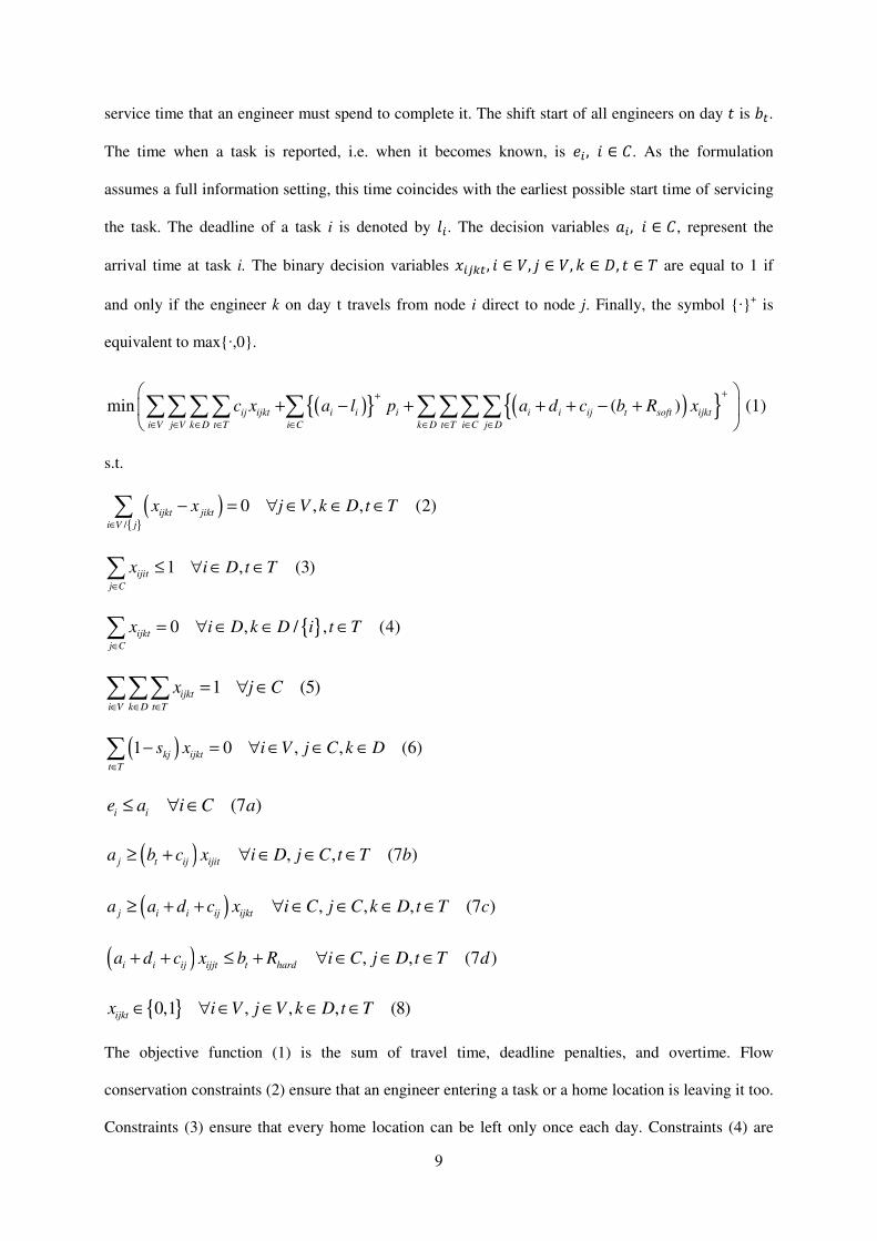
service time that an engineer must spend to complete it. The shift start of all engineers on day � is 0�.

The time when a task is reported, i.e. when it becomes known, is 1� , � ∈ . As the formulation

assumes a full information setting, this time coincides with the earliest possible start time of servicing

the task. The deadline of a task i is denoted by 2�. The decision variables 3�, � ∈ , represent the

arrival time at task i. The binary decision variables 4��, � ∈ �, � ∈ �, � ∈ �, � ∈ � are equal to 1 if

and only if the engineer k on day t travels from node i direct to node j. Finally, the symbol {·}+ is

equivalent to max{·,0}.

( ){ } ( ){ }min ( ) (1)ij ijkt i i i i i ij t soft ijkt

i V j V k D t T i C k D t T i C j D

c x a l p a d c b R x++

∈ ∈ ∈ ∈ ∈ ∈ ∈ ∈ ∈

+ − + + + − +

∑∑∑∑ ∑ ∑∑∑∑

s.t.

( ){ }/

0 , , (2)ijkt jikt

i V j

x x j V k D t T∈

− = ∀ ∈ ∈ ∈∑

1 , (3)ijit

j C

x i D t T∈

≤ ∀ ∈ ∈∑

{ }0 , / , (4)ijkt

j C

x i D k D i t T∈

= ∀ ∈ ∈ ∈∑

1 (5)ijkt

i V k D t T

x j C∈ ∈ ∈

= ∀ ∈∑∑∑

( )1 0 , , (6)kj ijkt

t T

s x i V j C k D∈

− = ∀ ∈ ∈ ∈∑

(7 )i i

e a i C a≤ ∀ ∈

( ) , , (7 )j t ij ijita b c x i D j C t T b≥ + ∀ ∈ ∈ ∈

( ) , , , (7 )j i i ij ijkta a d c x i C j C k D t T c≥ + + ∀ ∈ ∈ ∈ ∈

( ) , , (7 )i i ij ijjt t harda d c x b R i C j D t T d+ + ≤ + ∀ ∈ ∈ ∈

{ }0,1 , , , (8)ijktx i V j V k D t T∈ ∀ ∈ ∈ ∈ ∈

The objective function (1) is the sum of travel time, deadline penalties, and overtime. Flow

conservation constraints (2) ensure that an engineer entering a task or a home location is leaving it too.

Constraints (3) ensure that every home location can be left only once each day. Constraints (4) are

10

necessary for the assignment of engineers to their homes. Constraints (5) ensure that each task is

visited exactly once. Constraints (6) are the skill constraints. Constraints (7a) ensure that the arrival

time at a task will be after the task has been reported. Constraints (7b) and (7c) ensure that the arrival

time of an engineer at task j is after his departure time from his previous location plus the travel time

from the previous location to task j. Constraints (7d) ensure that the duration of a tour doesn’t exceed a

predefined amount. Separate sub-tour elimination constraints are not necessary since the calculation of

arrival times (constraints 7a–d) provide comparable functionality as node-potential-based sub-tour

elimination constraints, initially proposed by [30] for the Traveling Salesman Problem and used by

[22] for the Multi-Depot Vehicle Routing Problem. Constraints (8) impose binary values for the flow

variables 4��. This problem formulation has similarities to the multi-depot vehicle routing problem

[3], [6], [4].

Note that the formulation can be easily transformed into a MIP. The objective function can be

rewritten without the symbol {·}+ and the multiplication of decision variables in the third summand.

For this, we introduce auxiliary variables 5�, � ∈ and 6�� , � ∈ �, � ∈ � for the delay time of a task and

the overtime of an engineer on a given day respectively.

min (1')ij ijkt i i kt

i V j V k D t T i C k D t T

c x z p o∈ ∈ ∈ ∈ ∈ ∈ ∈

+ +

∑∑∑∑ ∑ ∑∑

(9)

( ) , (10)

0 (11)

0 , (12)

i i i

i i ij t soft ijjt jt

i C

i

jt

a l z i C

a d c b R x o j D t T

z i C

o j D t T

∈

≤ − ∀ ∈

+ + − − ≤ ∀ ∈ ∈

≥ ∀ ∈

≥ ∀ ∈ ∈

∑

The non-linear constraints (7c) and (7d) can be easily linearized too, since 4�� is binary [8]. Let 7 be

a large constant. Then (7c) and (7d) can be rewritten as:

(1 ) , , , (7 ')i i ij j ijkta d c a x M i C j C k D t T c+ + − ≤ − ∀ ∈ ∈ ∈ ∈

(1 ) , , (7 ')i i ij t hard ijjta d c b R x M i C j D t T d+ + − − ≤ − ∀ ∈ ∈ ∈

11

We have implemented the formulation with CPLEX 12.2, but could only solve some problems with up

to 3 engineers and 12 tasks in about an hour. But we also found instances of same size which caused

“out of memory” exceptions. We used an Apple iMac Core i7 2.93 GHz, model end of 2010.

4 Heuristics for the FSSP

Due to limited scalability of exact branch-and-cut approaches and the tight time limits for scheduling

which is performed every morning, we will now focus on heuristics to solve the FSSP. Several of

these heuristics are inspired by successful approaches to solving VRPs. We distinguish three types:

offline, online, and hybrid heuristics. Offline (or static) heuristics create a plan only once in the

morning and do not change it during the day. Online (or dynamic) heuristics assign the tasks

dynamically throughout the day. Hybrid heuristics combine both approaches. An initial plan is created

in the morning which can be changed during the day, but only if urgent tasks arise. Task duration and

the arrival of new tasks over time are the stochastic elements of FSSP which heuristics need to

consider. We work with estimates of service times and travel times rather than modeling the problem

as a stochastic optimization problem.

We have implemented a number of custom algorithms based on successful heuristics for the TSP and

VRP problems and also customized meta-heuristics for the FSSP, in order to find out if some

approaches dominate others. Our implementation is available upon request.

4.1 Objective function used in the heuristics

Every heuristic which compares costs incurred by the different candidate solutions (i.e., sets of routes)

it generates, uses the objective function presented above as the evaluation function with a main

adjustment. This is necessitated by the fact that, unlike classic VRPs, in FSSP the solution of each

heuristic must be evaluated on a daily basis, as routes are generated daily. In contrast to other VRPs

there is no constraint that every task must be visited. Therefore, solutions to a heuristic might just

postpone all tasks and thus minimize travel and overtime costs. However, field force engineers are

available and the planner should try to use their time efficiently each day. In this paper, we will

introduce costs for tasks that remain unassigned each day, so-called unassignment costs. These costs

12

are added to the evaluation function. Details on the individual parameters for our experiments will be

specified in Section 5.

4.2 Least Insertion Costs (LIC) and Conditional Least Insertion Costs (CLIC)

Tour-building insertion heuristics have been widely used for VRPs [40]. The next task to be assigned

is selected by means of a selection criterion, while the insertion criterion determines the best position

for insertion [41]. Our insertion heuristic for the FSSP, Least Insertion Costs (LIC), sorts the tasks

according to their due dates (selection criterion) and inserts them one by one in the position where the

insertion costs are minimal (insertion criterion). Let 8�9 denote the insertion costs defined as the

additional costs incurred by inserting task t between two adjacent nodes in engineer e’s route in the

best position. The best position is the one where the additional costs are minimal over all possible

insertion positions within the route of engineer e. Possible insertion positions are between two

adjacent nodes. We set 8�9 = ∞ if task t cannot be inserted in the route of e (due to skill or overtime

constraints). The task t is inserted in the route of the best engineer: e∗ = argmin (e) (8�9). The costs

of a route are calculated by using the evaluation function described in Section 4.1.

Conditional Least Insertion Costs (CLIC) is a variant of LIC, whereby the prefix “Conditional” refers

to the fact that it ignores a task from the actual daily planning if its unassignment costs are lower than

its actual insertion costs to the best possible route. Thus, the visit of a task will be postponed until the

day when an engineer passes close enough to the task or the task becomes urgent. In contrast, without

this condition, LIC assigns tasks whenever it is possible.

4.3 Opportunity Costs (OC, aka Regret – 3)

The OC heuristic, based on Ropke and Pisinger’s k-Regret algorithm [38], sorts the tasks in

descending order according to their opportunity costs and sequentially inserts them at their lowest-cost

insertion position, like LIC. Opportunity costs (regret measures) try to predict what will be lost if a

given task is not immediately inserted within its best route [35] and in the simplest case they are equal

to the difference in insertion costs between the second best and the best route. Note that each route is

assigned to an engineer, which means that opportunity costs are also a measure to be decided among

engineers. A generalized regret measure considering every alternative, e.g. not only the difference

13

between the second best and the best route but also between the third best and the best route, has been

used by Potvin and Rousseau for the VRPTW [35]. We implemented a variant of this regret measure

which considers differences between the three best engineers, since in our FSSP instances the tasks

can in most cases be assigned to one of the three best engineers: OC(t) = ∑ (8�# −G

HIJ 8�*), where 8�

#

denotes the insertion costs of task t to the route of its h-best engineer (an engineer has one route per

day). Considering more than three would weaken the “opportunity costs” notion of the measure. If 8�G

or 8�J are infinite, our heuristic does not consider them, but adds a constant value such that all tasks

with fewer available engineers have higher opportunity costs and thus are preferred. The reason is that

these tasks are more “constrained” and if their assignment is postponed, it may become impossible to

assign all of them.

The original k-Regret heuristic was designed for VRP problems without due dates and penalty costs.

Hence, we extended our heuristic to take these FSSP-specific properties into account. Our algorithm

divides all tasks into three sets according to their due dates, and then applies a separate run of the

default OC algorithm on each of them. During the first run only the most urgent tasks with a deadline

of less than 24 hours are considered. The second run processes tasks with a deadline expiring during

the next two days. Finally all remaining tasks are considered.

4.4 Heuristic Based on the Linear Assignment Problem (LAP)

The nonlinear generalized assignment problem has been used by VRP heuristics for clustering

purposes. After the clustering phase, the routing phase constructs routes by solving the TSP in each

cluster [10]. Our heuristic follows a new approach: It uses the well-known linear version of the

assignment problem2 to directly construct routes instead of the two-phase approach, which is not

applicable to the FSSP without extensive modifications (due to multiple depots, priorities, and skills).

In each iteration the LAP is efficiently solved using the Hungarian Algorithm [21] and each engineer

is assigned maximally one task. Afterwards, his current position is updated according to his assigned

task’s position. The costs of an assignment of a task to an engineer are set to the travel time between

the current position of the engineer and the position of the task. If an engineer doesn’t possess the skill

2 To underline this and avoid confusions with the assignment problem solved in Fisher and Jaikumar 1981, we call our heuristic Linear Assignment Problem instead of Assignment Problem.

14

to perform a task or his overtime after the assignment exceeds the limit of 30 minutes, costs are set to

infinity. The tasks are classified in due-date time intervals (e.g., 4 hours, 10 hours, 1 day, 3 days, all)

with the first one consisting of tasks of utmost urgency. During the first run only tasks having a due

date ending in four hours are considered. During the second run tasks of the second interval are

considered and so on. The granularity of the due-date time intervals directly influences to which extent

the deadlines vs. the travel times are optimized.

4.5 Hybrid Heuristic (HOC)

As a mixture between offline and online heuristics, we implemented a hybrid one which simulates the

behavior of a dispatcher, who plans routes in the morning and schedules urgent tasks on demand

throughout the day. This resembles the process in many companies: i) The dispatcher interferes only

when new urgent tasks emerge. Urgent tasks are those with a due date within 24 hours; ii) the

dispatcher can request the current position of an engineer; iii) the dispatcher always tries to assign

incoming urgent tasks to the closest engineer possessing the required skill; iv) if overtime restrictions

are violated, the dispatcher will postpone other tasks from the engineer’s schedule to the next day. For

initial routes HOC is based on the OC algorithm, due to the fact that OC outperformed other heuristics

without time-consuming post-optimization.

4.6 Post-Optimization: Variable Neighborhood Search (VNS)

Each heuristic that constructs tentative routes can additionally apply post-optimization to further

improve the solution. Post-optimization can be conducted on the initial schedule in the morning and

whenever the routes change in an online setting. We implemented a Variable Neighborhood Search

(VNS) [15], as there are a number of positive results in the recent literature [34]. For example, VNS

outperformed all other methods in an analysis of MDVRPTW, which is closely related to FSSP. The

use of a variety of neighborhoods enables a wide exploration of the search space and requires much

fewer parameters than for example tabu search [13],[14].

We implemented three types of the VNS which differ in the level of randomness regarding the search:

basic VNS, Variable Neighborhood Descent (VND), and Reduced VNS (RVNS). As RVNS has

shown to be better than the other VNS types on almost every simulation run, we will only report on

15

RVNS in this paper. During the “shaking” step of each iteration, RVNS randomly chooses a neighbor.

But in contrast to basic VNS, no local search is applied (hence the name Reduced VNS) and the move

is carried out if it leads to an improvement. This virtue proved to be decisive for our FSSP instances,

making RVNS the best post-optimization variant.

We now provide a succinct description of RVNS and comment on our concrete implementation for the

FSSP. As already mentioned, RVNS uses a variety of neighborhoods. A neighborhood of solution x

contains every solution reachable by the unique application of one operator on x. An operator

prescribes one or more moves to be applied on one or more routes of a solution. A move can be the

deletion of a task of a route, the insertion of a (previously unassigned) task to a route, or the relocation

or the swapping of tasks on an inter-route basis, i.e. between different routes and not within a single

route. K�(4) denotes the k-th neighborhood of the solution x (� = 1. . �+$,).

We implemented 15 neighborhoods, which are described in Appendix A. Their ordering can affect the

performance of the search [20]. The ordering which performed best in our experiments is based on the

Initialization:

Select the set of the neighborhood structures LM, M = N, … , MPQR which will be used in the

search

Find an initial solution R

Choose a stopping condition (e.g. maximum total running time, maximum time since last

improvement, maximum iterations, etc.)

Repeat the following until the stopping condition is met:

Set M = N

Until M = MPQR repeat the following steps:

Shaking: Generate a point RS at random from the neighborhood LM(R)

Move or not. If RS is better than the incumbent R, set R = RS and M = N; otherwise

set M = M + N

Figure 4-1: RVNS following Hansen et al. [15]

16

success rate of the neighborhoods and their size. When routes and tasks need to be selected in order to

generate a new solution, only routes and tasks located in close vicinity are considered. By the

calculation of distances between routes or a route and a task location, the center of gravity of the

routes is used. The center of gravity coordinates of a route are defined as the average coordinates of

the nodes it includes (the start and end-node are considered as two separate nodes although they

coincide). After the successful move from one solution to another, the TSP is solved to further

improve the affected routes. Note that the TSP uses the objective function outlined in Section 4.1. Our

implementation of RVNS stops after either the maximum running time or the maximum time since the

last improvement is reached.

4.7 Online Heuristics

All heuristics can operate both in offline and online modus. In the online mode though, adjustments

are necessary in order to dynamically handle new incoming tasks. Tentative routes are generated every

morning and updated through the day when a new task is reported. Firstly, the online heuristics try to

insert the new task in its lowest-cost insertion position. If this is impossible, for example because these

routes cannot be extended any more within a day, the online heuristics try to replace another task with

this one. This is only done if costs actually decrease. Hence, when the new task is urgent, it is very

likely to be exchanged with a non-urgent one. If a heuristic also implements the RVNS post-

optimization, the routes which are affected from the insertion of the new task as well as further routes

in close proximity are post-optimized for a limited amount of time. Considering further non-affected

routes is meaningful since the VNS prescribes inter-route neighborhoods and does not merely

optimize each route separately.

5 Research Design and Data

In this section we report on the design of experiments based on a dataset from our mobile phone

provider. The dataset contains the locations of 19,258 base stations, where tasks may emerge, and the

home locations of 177 technicians. We used travel time estimates between two locations based on the

Euclidean distance multiplied by an estimated average speed of 50 km/h, which has also been used by

17

our industry partner in the past. The service times were stochastic and heuristics worked with the

expected value.

The tasks in the dataset were classified in four categories determined by their nature and the given

service level agreements on which their due dates, priorities, and time windows are based (see Table

5-1). The time windows indicate when the tasks can be reported.3

Task Category Due Date Penalty

Factor

Time Window # Tasks

(I) service-affecting incident 4 h 10 00:00 – 24:00 5%

(II) non-service-affecting incident 24 h 5 00:00 – 24:00 45%

(III) service-affecting planned work 7 days 10 08:30 – 16:00 14%

(IV) non-service-affecting planned work

7 days 1 08:30 – 16:00 36%

Table 5-1: Task categories

There are also five types of skills. Tasks require a particular skill, while engineers possess particular

skills (Figure 5-1).

Figure 5-1: Skill distribution among task categories and engineers

Skill 0 is required by all tasks which are incidents. The remaining skills concern planned work like

integration or maintenance.

This led to the following independent variables in our experiments:

i) Position of the tasks and their report dates,

3 These time windows should not be confused with the time windows specified in classic VRPs, which state the earliest and latest possible time of visit of a task.

Skill 0

Skill 0

Skill 1

Skill 1Skill 2

Skill 3

Skill 3Skill 4

0% 20% 40% 60% 80% 100%

(I)

(II)

(III)

(IV)

Skill distribution among task

categories

Skill 0

Skill 1

Skill 2

Skill 3

Skill 4

0% 20% 40% 60% 80% 100%

Skill distribution among

engineers

18

ii) The mean and standard deviation of workload, which is defined by the number of tasks

per engineer and day, and is normally distributed,

iii) The mean and standard deviation of the duration of tasks which is normally distributed

and

iv) The percentage of high priority tasks which belong to category I (high priority).

Based on these independent variables we defined eight treatment combinations or scenarios and

conducted 20 repetitions with each of them (Table 5-2). The task positions and their arrival times are

chosen randomly for each repetition and all other parameters are fixed in a scenario. One repetition

simulates 14 days with new tasks throughout the day, but is extended up to 30 days until all tasks of

the first two weeks are finished.

Scenario # tasks 4 σσσσ # tasks 5 task duration σσσσ task duration Cat. I tasks6 Description

0 4 50 90 min 15 min 5% Base scenario

1 5 50 90 min 15 min 5% Increased workload

2A 4 50 90 min 1 min 5% More certainty about task duration

2B 4 50 90 min 30 min 5% Less certainty about task duration

3 4 150 90 min 15 min 5% Higher variance of tasks per day

4A 4 50 90 min 15 min 20% Increased urgent high priority tasks

4B 4 50 90 min 15 min 40% Increased urgent high priority tasks

5 8 50 30 min 15 min 5 % More tasks but lower task duration

Table 5-2: Independent variables in different scenarios (values different from base scenario underlined)

Scenario-0 (Base scenario): The base scenario describes the parameters that could also be found in

the data set of our industry partner. All 177 engineers are involved. Their shifts last from 08:00 am to

4:30 pm and during one day each worker has an average of four tasks to complete. The duration of the

tasks is drawn from a normal distribution with a mean of 90 minutes and a standard deviation of 15

minutes. Therefore, the targeted utilization level of the engineers is 71% (90min x 4 / 8,5h). The

4 Average number of tasks per engineer and day. 5 σ means standard deviation of a normally distributed variable. 6 Cat. I tasks are urgent tasks with high priority.

19

number of tasks is normally distributed with a standard deviation of 50 tasks (~7%). The percentages

of tasks belonging to each category can be found in Table 4-1.

Scenario-1 (Increased workload): To analyze the characteristics of the heuristics under high

workload, we increased the average number of tasks per engineer and day to five tasks. The targeted

utilization level is 88%. The spatial distribution of the tasks has a significant impact on the utilization.

Scenario-2A (Low variability of task duration): The standard deviation for drawing the real task

duration is set to one minute, instead of 15 minutes in the base scenario. In other words, task duration

is very predictable.

Scenario-2B (High variability of task duration): In contrast to Scenario-2A, the deviation of the

service time is now increased to 30 minutes.

Scenario-3 (High variance of the number of tasks per day): In this scenario the variance of the

number of tasks per day is increased (standard deviation of 150 tasks). It can happen that the engineers

cannot be fully occupied one day due to a lack of available tasks and another day they may not be able

to keep up with the workload. Such fluctuations can happen if operators want to carry out a large

number of technical updates on the base stations in one period, or due to weather conditions.

Scenario-4A (20% urgent tasks with high priority): The percentage of high priority tasks (service-

affecting incidents) is increased from 5% to 20%. Thus the degree of dynamism of the scenario

increases drastically, as more tasks are reported during the day and require immediate attention. This is

a very relevant scenario for the mobile phone operator as the percentage of disturbances may increase

drastically due to weather or other conditions.

Scenario-4B (40% urgent tasks with high priority): The percentage of high priority tasks is further

increased to 40%.

Scenario-5 (More tasks but shorter service time): This scenario differs substantially from the others

as it contains many more tasks with shorter service durations. The number of tasks per day is doubled

and the service duration reduced to 30 minutes. The targeted utilization level is only 47% while the

distance to be covered by the engineers increases. We want to understand if the results of the initial

20

scenarios carry over to workforce scheduling problems, where each traveling employee completes

many short tasks per day.

To calculate the unassignment costs in our experiments, we assume that each unassigned task will be

visited in 24 hours (which may lead to additional deadline penalties) and cause 100 minutes of

additional travel time. These values could be further optimized by using past data, e.g. by calculating

the average additional travel time per task. Additionally, if the overtime of a route exceeds 30 minutes,

the costs of the routes are set to infinity in order to avoid routes with larger overtime. Of course, the

final overtime after executing a plan may exceed 30 minutes due to the fact that the real task duration

deviates from the estimate.

6 Results

To evaluate our computational results we use the objective function introduced in Section 3. In

addition to the objective function values, we report on travel time and deadline penalties individually

when appropriate. The calculation of deadline penalties is based on the delay and category of each task

(see Section 3). We tested dozens of heuristics and heuristic combinations (e.g. next neighbor

algorithms with different proximity measures which consider both spatial distance and deadlines or

only one of them, cluster first route second algorithms, and RVNS, VNS, VND with different

parameters and different initial solutions such as OC, LAP, etc.), but due to space restrictions we

report only on the results of the best ones. The net computation time needed to run the presented

experiments was 1660 hours on eight identical PCs (Intel Core 2, 2.67GHz, 4GB).

6.1 Overall Comparison: Online vs. Offline vs. Hybrid

Firstly, we note that there are dominance relationships among the heuristics across all repetitions in the

sense that the rank of each particular heuristic stays mostly the same from repetition to repetition (the

corresponding diagram can be found in Appendix B). This observation underpins the robustness of the

results.

21

Table 6-1 provides an overview of the average values of the offline heuristics in the base scenario and

Table 6-2 of the online and hybrid heuristics. The unit of measure is minutes, as explained in Section

3.

Table 6-1: Offline heuristics’ averages on the base scenario

Table 6-2: Online and hybrid heuristics’ averages on

the base scenario

Offline heuristics lead to much higher costs (i.e. objective function values) than the online heuristics.

The costs of the hybrid heuristic are close to the costs of the online heuristics. Compared to the best

offline heuristic, HOC incurs only 39% of its costs and dominates it in every metric, including running

times (see Appendix C). The largest part of the costs in offline heuristics, around 80% on average, is

due to deadline penalties, which cannot be avoided because new and urgent tasks emerging throughout

the day could not be considered immediately. In contrast, online heuristics incur much lower penalties

and hence the largest part of their costs is due to travel time. Although one could expect travel time to

increase in online heuristics, as deadlines of urgent tasks need to be considered, the travel times of OC,

LAP, and LIC are even lower in the online setting of the base scenario.

We will now compare the best online heuristic, OCnRVNS7, the best offline heuristic, which is again

OCnRVNS, and the hybrid heuristic, HOC. The comparison is conducted on the base scenario and on

scenarios 4A and 4B, where the percentage of urgent high priority tasks (category I) increases. This

change should have a considerable impact on the comparison between the offline, hybrid, and the

online heuristics.

7 RVNS with OC as start solution.

Heuristic Obj. function value Travel time Penalties

OCnRVNS 1,660,387 247,921 1,391,598

OC 1,702,559 282,729 1,393,506

CLIC 1,756,122 333,360 1,391,620

LAP 1,799,679 379,067 1,400,126

LIC 1,813,992 382,308 1,396,385

Heuristic Obj.function Travel time Penalties

OCnRVNS 451,900 248,027 186,128

LICnRVNS 452,629 252,616 182,231

OC 498,557 274,609 203,923

LAP 546,295 367,659 162,445

LIC 582,115 351,028 211,044

HOC 649,475 245,707 388,621

22

Figure 6-1: Objective function of best online, best offline, and hybrid heuristic

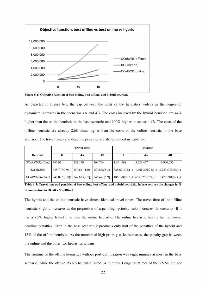
As depicted in Figure 6-1, the gap between the costs of the heuristics widens as the degree of

dynamism increases in the scenarios 4A and 4B. The costs incurred by the hybrid heuristic are 44%

higher than the online heuristic in the base scenario and 100% higher in scenario 4B. The costs of the

offline heuristic are already 2.68 times higher than the costs of the online heuristic in the base

scenario. The travel times and deadline penalties are also provided in Table 6-3.

Heuristic

Travel time Penalties

0 4A 4B 0 4A 4B

OCnRVNS(offline) 247,921 253,179 264,764 1,391,598 5,529,457 10,900,636

HOC(hybrid) 245,707(0.9↓) 250,641(1.0↓) 250,868(5.3↓) 388,621(72.1↓) 1,461,296(73.6↓) 3,223,505(70.6↓)

OCnRVNS(online) 248,027 (0.0↑) 247,633(2.2↓) 246,471(6.9↓) 186,128(86.6↓) 697,929(87.9↓) 1,478,210(86.4↓)

Table 6-3: Travel time and penalties of best online, best offline, and hybrid heuristic. In brackets are the changes in %

in comparison to OCnRVNS(offline).

The hybrid and the online heuristic have almost identical travel times. The travel time of the offline

heuristic slightly increases as the proportion of urgent high-priority tasks increases. In scenario 4B it

has a 7.5% higher travel time than the online heuristic. The online heuristic has by far the lowest

deadline penalties. Even in the base scenario it produces only half of the penalties of the hybrid and

13% of the offline heuristic. As the number of high priority tasks increases, the penalty gap between

the online and the other two heuristics widens.

The runtime of the offline heuristics without post-optimization was eight minutes at most in the base

scenario, while the offline RVNS heuristic lasted 64 minutes. Longer runtimes of the RVNS did not

0

2,000,000

4,000,000

6,000,000

8,000,000

10,000,000

12,000,000

0 4A 4B

Objective function, best offline vs best online vs hybrid

OCnRVNS(offline)

HOC(hybrid)

OCnRVNS(online)

improve the results significantly. The online heuristics without post

minutes and the online RVNS heuristics 172 minutes (that is about 12 minutes per simulated day

analysis simulating 14 days). All

We will now examine the performance of the offline and online heuristics separately.

6.2 Offline Heuristics in the B

Figure 6-2 illustrates the performance of the offline heuristics on the base scenario with regar

component of the objective function. The percentages,

of each heuristic’s objective function value from the value of the best offline heuristic.

Figure 6-2: Offline heuristics, base scenario

The best heuristic is the one with post

optimization (OC). Their lower costs are mainly due to their shorter travel times, although the travel

time accounts for only 20% of the total costs. The de

heuristic to heuristic; the worst heuristic

one. This also demonstrates the difficult

without knowledge about future tasks

OCnRVNS (2.54%), which is ascribed only to

8 The deviation is computed with the following formula:

23

improve the results significantly. The online heuristics without post-optimization

minutes and the online RVNS heuristics 172 minutes (that is about 12 minutes per simulated day

All running times can be found in Appendix C.


Base Scenario

2 illustrates the performance of the offline heuristics on the base scenario with regar

the objective function. The percentages, to the right of the bars, represent the deviation


: Offline heuristics, base scenario

The best heuristic is the one with post-optimization (OCnRVNS) followed by its version without post


time accounts for only 20% of the total costs. The deadline penalties do not vary significantly from

heuristic to heuristic; the worst heuristic with respect to penalties deviates only 0

difficulty of further decreasing deadline penalties in the offline world

without knowledge about future tasks and leads to a low improvement of the total cost from OC to

54%), which is ascribed only to the decrease in travel time.

The deviation is computed with the following formula: /1U�3��6�(V1WX�(�� V� � $Y9%$Z9

optimization lasted at most 30

minutes and the online RVNS heuristics 172 minutes (that is about 12 minutes per simulated day in an


2 illustrates the performance of the offline heuristics on the base scenario with regard to each

the bars, represent the deviation8


optimization (OCnRVNS) followed by its version without post-


adline penalties do not vary significantly from

penalties deviates only 0.61% from the best

deadline penalties in the offline world

and leads to a low improvement of the total cost from OC to

$Y9%$Z9�#�[ \]^_` $Y9%$Z9�#`�

\]^_` $Y9%$Z9�#`�

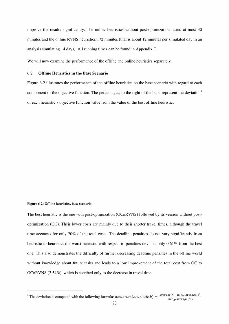
6.3 Comparison of Offline H

In the following we analyze whether the results of the base scenario carry over to other scenarios.

Table 6-3 compares the performance of the heuristics as deviation from the best ones (marked as

0.00%) in each scenario.

Deviations of objective function 0

LIC 9.25%

CLIC 5.77%

OC 2.54%

OCnRVNS 0.00%

LAP 8.39%

Table 6-3: Deviations (in %) from best heuristic, offline heuristics, all scenarios

OCnRVNS always performs best followed either by the OC or the CLIC. Note that the ranking of the

heuristics OCnRVNS > OC > CLIC >

in all scenarios except 1 and 4B, where OC < CLIC. CLIC always

the usage of unassignment costs. This is important, since unassignment costs

in the post-optimization.

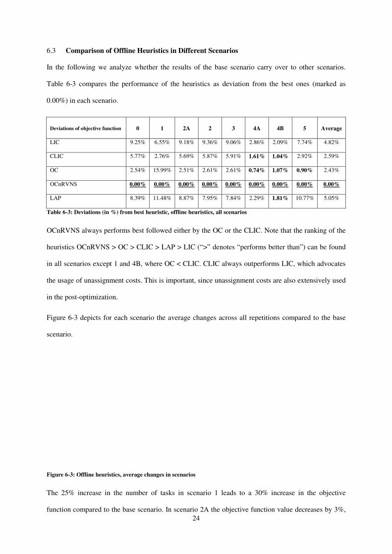
Figure 6-3 depicts for each scenario the average changes across all repetitions compared to the base

scenario.

Figure 6-3: Offline heuristics, average changes in scenarios

The 25% increase in the number of tasks in

function compared to the base scenario. In scenario 2A the objective function value decreases by 3%,

24

Heuristics in Different Scenarios

whether the results of the base scenario carry over to other scenarios.

3 compares the performance of the heuristics as deviation from the best ones (marked as

1 2A 2 3 4A 4B

25% 6.55% 9.18% 9.36% 9.06% 2.86% 2.09%

77% 2.76% 5.69% 5.87% 5.91% 1.61% 1.04%

54% 15.99% 2.51% 2.61% 2.61% 0.74% 1.07%

00% 0.00% 0.00% 0.00% 0.00% 0.00% 0.00%

39% 11.48% 8.87% 7.95% 7.84% 2.29% 1.81%

3: Deviations (in %) from best heuristic, offline heuristics, all scenarios


CLIC > LAP > LIC (“>” denotes “performs better than”) can be found

1 and 4B, where OC < CLIC. CLIC always outperforms LIC

. This is important, since unassignment costs are also

for each scenario the average changes across all repetitions compared to the base

3: Offline heuristics, average changes in scenarios

increase in the number of tasks in scenario 1 leads to a 30% increase in the objective


whether the results of the base scenario carry over to other scenarios.

3 compares the performance of the heuristics as deviation from the best ones (marked as

4B 5 Average

09% 7.74% 4.82%

04% 2.92% 2.59%

07% 0.90% 2.43%

00% 0.00% 0.00%

81% 10.77% 5.05%


“performs better than”) can be found

LIC, which advocates

are also extensively used

for each scenario the average changes across all repetitions compared to the base

increase in the objective


which is due to savings produced by the lower variance of the

2B, the objective function increases

per day leads to a 3% increase in total costs. When the volume of very urgent tasks (deadlines in

hours) increases to 20% and 40% (instead of 5%) in

function values increase by 237% and 548% respectively. This is a result of the fact that tasks with

short deadlines cannot be considered immediately when planning tasks offline every morning. Finally,

in scenario 5 the objective function value increases on average 81% due to the difficulty

time the increased number of tasks (96% increase in deadline penalties). Travel time only increases by

30%.

6.4 Online Heuristics

Figure 6-4 depicts the performance of the online heuristics relative to each other in the base scenario 0.

Figure 6-4: Online heuristics, base scenario

Two groups of heuristics can be identified. The first group consists of heuristics with post

optimization, which dominate the second group of

heuristic of the second group and deviates about 10% from the first group.

optimization in the online world is

2.54%). In contrast to the offline setting, online heuristics optimize routes not only in the morning but

during the whole day.

25

produced by the lower variance of the task duration. In contrast, in scenario

B, the objective function increases by 3%. In scenario 3 the stronger variance in the number of tasks

per day leads to a 3% increase in total costs. When the volume of very urgent tasks (deadlines in

hours) increases to 20% and 40% (instead of 5%) in scenarios 4A and 4B respectively, the objective



nario 5 the objective function value increases on average 81% due to the difficulty

increased number of tasks (96% increase in deadline penalties). Travel time only increases by

4 depicts the performance of the online heuristics relative to each other in the base scenario 0.

4: Online heuristics, base scenario

Two groups of heuristics can be identified. The first group consists of heuristics with post

the second group of heuristics without post-optimization. OC is the best

heuristic of the second group and deviates about 10% from the first group. The contribution of post

optimization in the online world is therefore four times higher than in the offline world (

. In contrast to the offline setting, online heuristics optimize routes not only in the morning but

task duration. In contrast, in scenario

3%. In scenario 3 the stronger variance in the number of tasks

per day leads to a 3% increase in total costs. When the volume of very urgent tasks (deadlines in four

scenarios 4A and 4B respectively, the objective



nario 5 the objective function value increases on average 81% due to the difficulty of handling in

increased number of tasks (96% increase in deadline penalties). Travel time only increases by

4 depicts the performance of the online heuristics relative to each other in the base scenario 0.

Two groups of heuristics can be identified. The first group consists of heuristics with post-

optimization. OC is the best

he contribution of post-

n the offline world (10.32% vs.

. In contrast to the offline setting, online heuristics optimize routes not only in the morning but

26

Interestingly, the quality of the start solution has little impact on the final solution when using post-

optimization. The two RVNS heuristics yield almost the same results although the starting solution of

OC is better than the starting solution of LIC.

With respect to travel time, the best heuristics are again the ones with the RVNS post-optimization and

the best one of the remaining heuristics is the OC. The worst heuristic is LAP due to its due-time

intervals that put an emphasis on deadlines. This is the reason why this heuristic has the lowest

deadline penalties.

6.5 Comparison of Online Heuristics in Different Scenarios

Again, we compare the robustness of the results by analyzing scenarios 1 to 5. Table 6-4 shows the

performance of the heuristics in terms of deviation from the best result.

Deviations of

objective

function 0 1 2A 2B 3 4A 4B 5 Average

LAP 20.89% 4.61% 32.04% 3.36% 10.32% 5.04% 9.34% 25.81% 10.83%

LIC 28.81% 49.56% 33.64% 15.77% 22.00% 23.90% 24.82% 9.88% 25.83%

OC 10.32% 18.97% 8.80% 3.09% 6.95% 9.98% 7.20% 10.22% 8.88%

OCnRVNS 0.00% 0.85% 0.00% 2.67% 0.00% 0.00% 0.00% 0.00% 0.00%

LICnRVNS 0.16% 0.00% 2.00% 0.00% 0.28% 2.84% 1.01% 1.18% 0.67%

Table 6-4: Deviations (in %) from best heuristic, online heuristics, all scenarios

In the online setting, the best heuristics are always the ones with post-optimization, whereby

OCnRVNS achieves the best result in all but two scenarios. The best heuristic without post-

optimization on average is the OC, as in the offline setting.

Figure 6-5 depicts for each scenario the average changes across all heuristics and repetitions compared

to the base scenario.

Figure 6-5: Online heuristics, average changes in scenarios

In scenario 1 the number of tasks increases by 25% and le

objective function value due to the high increase in deadline penalties. In scenario 2A the objective

function value decreases by 13% while in 2B it increases

offline heuristics. Hence, the accurate prediction of the task duration is more important in an online

setting. The reason is presumably that in the online world the information ab

task, which is revealed upon task completion,

the tour. In scenario 3, the stronger variance of the

scenarios 4A and 4B, which prescribe

respectively. These numbers are much lower than in the offline setting. In scenario 5, the objective

function value stays almost the same

online heuristics can handle scenarios with many more tasks of short duration much better.

7 Conclusions

Maintenance and repair jobs at base stations of

problem in the telecom industry. This problem

case of vehicle routing problems

field service scheduling solutions are available

about the location of each engineer and allow for dynamic scheduling

27

average changes in scenarios

In scenario 1 the number of tasks increases by 25% and leads to an average increase of 62


3% while in 2B it increases by 18%. These values were higher than with

, the accurate prediction of the task duration is more important in an online

setting. The reason is presumably that in the online world the information about the real duration of a

, which is revealed upon task completion, can be exploited by adjusting the remaining schedule of

the tour. In scenario 3, the stronger variance of the number of tasks leads to an increase of 4%. In

prescribe more high priority tasks, total costs increase


stays almost the same, whereas in the offline setting it increases by


base stations of mobile phone operators lead to a widespread

. This problem has not been described in the literature, but is

vehicle routing problems as can be found in other service industries as well

scheduling solutions are available on the market which provide real

about the location of each engineer and allow for dynamic scheduling of tasks throughout the day

ads to an average increase of 62% in the


%. These values were higher than with

, the accurate prediction of the task duration is more important in an online

out the real duration of a

can be exploited by adjusting the remaining schedule of

tasks leads to an increase of 4%. In

increase by 106% and 273%


by 81%. Therefore, the


a widespread planning

has not been described in the literature, but is a special

as well. Nowadays, mobile

ovide real-time information

of tasks throughout the day. In

28

this paper, we want to understand the efficiency gains of having this information available as

compared to daily offline scheduling every morning, which is a widespread practice.

For this purpose, we first defined the field service scheduling problem with priorities (FSSP) as a

mixed integer program and described its relation to other vehicle routing and planning problems. FSSP

has similarities to the Multi-Depot Vehicle Routing Problem with Time Windows, but also distinct

differences which have an impact on the design and the performance of the heuristics in solving the

problem. We introduced a variety of offline and online heuristics for this new problem, which are

based on successful approaches to other vehicle routing problems. These algorithms were evaluated

based on a real-world data set and on different scenarios in order to understand the robustness of the

results.

The best heuristics were the ones adding the post-optimization heuristic Reduced Variable

Neighborhood Search (RVNS), which outperformed other post-optimization routines (such as basic

VNS and VND). The contribution of RVNS was also significant in the online world, where deadline

penalties were lower. RVNS improved the best heuristic (OC) by more than 10% and other heuristics

such as LIC by more than 25%. The results were robust against modifications of the base scenario.

The best offline and online heuristics were compared to each other and to a hybrid heuristic. The

results of this comparison indicate that online heuristics lead to substantially lower costs than pure

offline heuristics, which is also due to the deadline penalties in our objective function. Even without

such penalties the differences are significant. Travel times are often also lower when using online

heuristics.

Interestingly, the hybrid heuristic achieves considerably lower total costs than the offline heuristics. It

is close to the costs of online heuristics, especially when the degree of dynamism is low. The hybrids

simulate the planning process in companies where all routes are planned in the morning, but a

dispatcher assigns urgent tasks. This indicates that if a skilled dispatcher is available in a company

which plans the routes once a day and assigns urgent jobs throughout the day, the savings in travel and

overtime costs might be lower and an operator needs to weigh the investment and maintenance costs

for the mobile workforce management solution and the costs of manual intervention. In mobile

29

workforce management systems, the effort of the human dispatchers will be much reduced, as urgent

tasks are handled and assigned automatically. Note that additional costs for introducing and

maintaining mobile field service scheduling systems or manual dispatching have not been considered

in this paper as they tend to vary considerably and we only focus on efficiency gains in routing the

engineers. These costs are typically known in at the time of deciding between a mobile field service

scheduling and a manual dispatching solution. Our study can help calculating each business case by

providing estimates of the efficiency gains of one system over the other.

8 References

[1] R. Baldacci, A. Mingozzi, A unified exact method for solving different classes of vehicle

routing problems, Mathematical Programming, Vol.120, (2009) 347-380.

[2] D. Bertsimas, G. Van Ryzin, A Stochastic and Dynamic Vehicle Routing Problem in the

Euclidean Plane, Operations Research, Vol.39, (1991) 601-615.

[3] L. Bodin, A. Assad, M. Ball, Routing and Scheduling of Vehicles and Crews - The State of the

Art, Computers and Opertions Research, Special Issue, Vol. 10, No. 2, (1983) 63-212.

[4] J.-F. Cordeau, M. Gendreau, G. Laporte, A Tabu Search Heuristic for Periodic and Multi-

Depot Vehicle Routing Problems, Networks, Vol. 30, (1997) 105-119.

[5] J.F. Cordeau, G. Laporte, A. Mercier, An Improved Tabu Search Algorithm for the

Handling of Route Duration Constraints in Vehicle Routing Problems with Time Windows,

Journal of the Operational Research Society, Vol.55, (2004) 542-546.

[6] T.G. Crainic, G. Laporte, Fleet Management and Logistics, (Kluwer Academic Publishers,

1998).

[7] G.B. Dantzig, J.H. Ramser, The Truck Dispatching Problem, Management Science, Vol.6,

(1959) 80-91.

[8] J. Desrosiers, Y. Dumas, M.M. Solomon and F. Soumis, Time Constrained Routing and

Scheduling, in: T.L.M. Ball M.O., C.L. Monma, G.L. Nemhauser Ed. Handbooks in Operations

Research and Management Science 8: Network Routing, (Elsevier Science Publishers,

Amsterdam, 1995), pp. 35–139.

[9] A.T. Ernst, H. Jiang, M. Krishnamoorthy, D. Sier, Staff scheduling and rostering: A review

of applications, methods and models, European Journal of Operational Research, Vol.153,

(2004) 3-27.

[10] M. Fisher, M. Jaikumar, A Generalized Assignment Heuristic for Vehicle Routing,

Networks, Vol. 11, (1981) 109-124.

[11] T. Flatberg, G. Hasle, O. Kloster, E.J. Nilssen, A. Riise, Dynamic and Stochastic Vehicle

Routing in Practice, in: Dynamic Fleet Management, (Springer. Operations Research /

Computer Science Interfaces, 2007), pp. 45-68.

[12] G. Ghiani, F. Guerriero, Real-time vehicle routing: Solution concepts, algorithms and

parallel computing strategies, European Journal of Operational Research, Vol.15, (2003) 1-11.

[13] F. Glover, Tabu Search — Part I, ORSA Journal on Computing, Vol.1, (1989) 190-206.

[14] F. Glover, Tabu Search — Part II, ORSA Journal on Computing, (1990) 4-32.

30

[15] P. Hansen, N. Mladenovic, Variable Neighborhood Search: Principles and Applications,

Journal of Operational Research, Vol. 130, (2001) 449–467.

[16] F.T. Hanshar, B.M. Mobuki-Berman, Dynamic vehicle routing using genetic algorithms,

Applied Intelligence, Vol. 27, (2007) 89-99.

[17] HEC Montreal, www.hec.ca/chairedistributique/data, (2010).

[18] C. Heimerl, R. Kolisch, Scheduling and staffing multiple projects with a multi-skilled

workforce, OR Spectrum, (2009) 1-26.

[19] P. Hofstedt, A. Wolf, Einführung in die Constraint-Programmierung, (Springer, Berlin,

Heidelberg, 2007).

[20] B. Hu, G.R. Raidl, Variable neighborhood descent with self-adaptive neighborhood-

ordering, in: Proceedings of the 7th EU/MEeting on Adaptive, Self-Adaptive, and Multi-Level

Metaheuristics, (Malaga, Spain, 2006).

[21] H.W. Kuhn, The Hungarian method for the assignment problem, in: Naval Research

Logistic Quarterly, Vol.2, (1955), pp. 83-97.

[22] R.V. Kulkarni, P.R. Bhave, Integer programming formulations of vehicle routing problems,

European Journal of Operational Research, Vol.20, (1985) 58-67.

[23] G. Laporte, Y. Nobert, D. Arpin, Optimal solutions to capacitated multidepot vehicle

routing problems, Congressus Numerantium, 44(1984) 283-292.

[24] G. Laporte, Y. Nobert, S. Taillefer, Solving a family of multi-depot vehicle routing and

allocation problems, Transportation Science, 22(1988) 161-172.

[25] A. Larsen, O. Madsen, M. Solomon, Partially Dynamic Vehicle Routing - Models and

Algorithms, Journal of the Operational Research Society, Vol.38, (2002) 637-646.

[26] D. Lesaint, C. Voudouris, N. Azarmi, "Dynamic Workforce Scheduling for British

Telecommunications plc., Interfaces, Vol.30, (2000) 45-56.

[27] D. Lesaint, C. Voudouris, N. Azarmi, I. Alletson, B. Laithwaite, Field Workforce

Scheduling, BT Technology, Vol.21, (2003) 23-26.

[28] K. Lund, O. Madsen, J.M. Rygaard, Vehicle routing problems with varying degrees of

dynamism, Insititute of Mathematical Modelling, Technical University of Denmark, (1996).

[29] M. Maoz, Magic Quadrant for Field Sevice Management, Gartner Research, (2008).

[30] C.E. Miller, A.W. Tucker, R.A. Zemlin, Integer Programming Formulation, Journal of the

ACM, Vol. 7, (1960) 326-329.

[31] S. Mitrovic-Minic, R. Krishnamurti, G. Laporte, The double-horizon heuristic for the

dynamic pickup and delivery problem with time windows, Transportation Science, Vol.38,

(2004) 669-685.

[32] D. Pisinger, S. Ropke, A general heuristic for vehicle routing problems, Computers &

Operations Research, Vol.34, (2007) 2403-2435.

[33] M. Polacek, S. Benkner, K. Doerner, R.F. Hartl, A Cooperative and Adaptive Variable

Neighborhood Search for the Multi Depot Vehicle Routing Problem with Time Windows,

Business Research, Vol. 1, (2008) 207-218.

[34] M. Polacek, R.F. Hartl, K. Doerner, A variable neighborhood search for the multi depot

vehicle routing problem with time windows, Journal of Heuristics, Vol. 10, (2004) 613-627.

[35] J.Y. Potvin, J.M. Rousseau, A parallel route building algorithm for the vehicle routing and

scheduling problem with time windows, European Journal of Operational Research, Vol. 66

(1993) 331-340.

31

[36] H. Psaraftis, Dynamic vehicle routing problems, in: Vehicle Routing: Methods and Studies,

(Elsevier, North-Holland, 1988), pp. 223-248.

[37] S. Ropke, D. Pisinger, A unified heuristic for a large class of vehicle routing problems with

backhauls, European Journal of Operational Research, Vol.171, (2004) 750-775.

[38] S. Ropke, D. Pisinger, An Adaptive Large Neighborhood Search Heuristic for the Pickup

and Delivery Problem with Time Windows, Transportation Science, (2006) 455-472.

[39] M. Savelsbergh, M. Sol, The General Pickup and Delivery Problem, Transportation

Science, Vol.29, (1995) 17-29.

[40] M. Solomon, Algorithms for the Vehicle Routing and Scheduling Problems with Time

Window, Operations Research, Vol. 35, (1987) 254-265.

[41] A. Van Breedam, A parametric analysis of heuristics for the vehicle routing problem with

side-constraints, European Journal of Operational Research, Vol. 137, (2002) 348-370.

[42] M.C. Wu, S.H. Sun, A project scheduling and staff assignment model considering learning

effects, International Journal of Advanced Manufacturing Technology, Vol.28, (2006) 1190-

1195.

Appendix A: Neighborhoods in RVNS

Our neighborhoods are divided into two large categories, depending on whether they are allowed to

change the status of a task from unrouted (i.e. not yet planned in a route) to routed (and vice versa) or

not. The first category is labeled “UR” (Unrouted, Routed) and the second with “IR” (Inter-Route). In

the following table A-1, the neighborhoods together with their size are listed (m denotes the number of

unassigned tasks considered, k the number of tasks in a route, and R1, R2, R3 denote routes). As

already mentioned, the routes considered by a neighborhood are selected randomly. As a first

exemplary calculation of the size, consider the neighborhood UR1_Insert_1. We have m unassigned

tasks which can be inserted at k possible positions. Hence its size is O(k x m).

UR1_Insert_1 insert one unrouted task to R1 O(k x m)

UR1_Remove_1 remove a routed task from R1 O(k)

UR1_Swap_1 remove a routed task from R1 and insert an unrouted task to R1

O(k2 x m)9

UR1_Swap_2 remove two routed tasks from R1 and insert two unrouted tasks to R1

O(2k3 x m2) 10

UR1_Swap_21 remove one routed task from R1 and insert two unrouted tasks to R1

O(2k2 x m2)

9 Note that the insertion position of the unrouted task must not be the position of the task to be removed. This holds for every neighborhood where tasks are swapped. 10 Exemplary calculation: Selection of two routed tasks costs O(k2), selection of two unrouted tasks O(m2), then the two unrouted tasks are inserted O(k+k) (the insertions occur sequentially and each one costs O(k)), all together O(k2 x m2 x 2k) = O(k3 x m2).

UR1_Swap_12 remove two routed tasks from R1 and insert one unrouted task to R1

UR2_Relocate_1 insert an unrouted task to R1, move a task from R1 to R2

UR2_Swap_1 insert an unrouted task to R1, move a task from R1 to R2, remove a task from R2

IR2_Relocate_1 move a task from R1 to R2

IR2_Swap_1 move a task from R1 to R2 and a task from R2 to R1

IR2_Relocate_2 move two tasks from R1 to R2

IR2_Swap_2 move two tasks from R1 to R2 and two tasks from R2 to R1

IR2_Swap_12 move one task from R1to R2 and two tasks from R2 to R1

IR3_Relocate_1 move a task from R1 to R2 and a task from R2 to R3

IR3_Swap_1 move a task from R1 to R2, a task from R2 to R3 and a task from R3 to R1

Table A-1: Neighborhoods

Appendix B: Performance of all

Repetitions of B

The intention of the plot (Figure B

repetitions of the base scenario. It can be observed

mostly the same from repetition to repetition

heuristics, which perform very similar

setting.

Figure B-1: 20 Repetitions of the base scenario

32

remove two routed tasks from R1 and insert one unrouted

insert an unrouted task to R1, move a task from R1 to R2

insert an unrouted task to R1, move a task from R1 to R2, remove a task from R2

move a task from R1 to R2

move a task from R1 to R2 and a task from R2 to R1

move two tasks from R1 to R2

move two tasks from R1 to R2 and two tasks from R2 to R1

move one task from R1to R2 and two tasks from R2 to R1

move a task from R1 to R2 and a task from R2 to R3

move a task from R1 to R2, a task from R2 to R3 and a task from R3 to R1

: Performance of all Heuristics on the

Base Scenario

igure B-1) is to analyze the robustness of the results across the 20

repetitions of the base scenario. It can be observed that the rank of each particular heuristic stays

repetition to repetition. Most line intersections are due to the two RVNS

which perform very similarly since the initial solution (OC or LIC) is not decisive in our

1: 20 Repetitions of the base scenario

remove two routed tasks from R1 and insert one unrouted O(k3 x m)

O(k2 x m)

insert an unrouted task to R1, move a task from R1 to R2, O(k3 x m)

O(k2)

O(k3)

O(k2)

O(k5)

O(k4)

O(k3)

move a task from R1 to R2, a task from R2 to R3 and a task O(k4)

euristics on the Twenty

the robustness of the results across the 20

the rank of each particular heuristic stays

intersections are due to the two RVNS

since the initial solution (OC or LIC) is not decisive in our

33

Appendix C: Additional results

Heuristic Std dev Std dev / Average

LAP (on) 31,400.24 5.75%

LIC (off) 127,853.66 7.05%

LAP (off) 132,033.26 7.34%

CLIC (off) 131,761.42 7.50%

OC (off) 131,070.84 7.70%

OCnRVNS (off) 132,190.58 7.96%

LIC(on) 49,805.58 8.56%

OC (on) 43,973.62 8.82%

HOC (hybrid) 64,269.35 9.90%

LICnRVNS (on) 44,840.36 9.91%

OCnRVNS (on) 46,701.98 10.33%

Table C-1: Standard deviation of all heuristics on the base scenario

OFFLINE – Objective function values for each scenario

0 1 2A 2B 3 4A 4B 5

LIC 1,813,992 2,257,012 1,758,251 1,876,891 1,866,873 5,970,392 11,422,207 3,263,036

LAP 1,799,679 2,361,475 1,753,234 1,852,671 1,846,094 5,937,132 11,390,898 3,354,722

CLIC 1,756,122 2,176,706 1,701,998 1,817,065 1,813,062 5,897,958 11,305,291 3,117,120

OC 1,702,559 2,456,980 1,650,788 1,761,002 1,756,526 5,847,359 11,309,059 3,055,724

OCnRVNS 1,660,387 2,118,231 1,610,398 1,716,263 1,711,830 5,804,237 11,188,785 3,028,546

Table C-2: Objective function of offline heuristics, all scenarios

OFFLINE – Travel time for each scenario

0 1 2A 2B 3 4A 4B 5

LIC 382,308 487,821 349,444 408,839 389,188 380,982 374,273 528,046

LAP 379,067 458,718 346,922 405,325 380,298 363,227 367,693 592,356

CLIC 333,360 442,204 300,376 359,746 346,132 332,510 327,945 387,706

OC 282,729 346,002 249,803 308,715 288,068 287,246 291,985 312,936

OCnRVNS 247,921 312,679 214,509 273,636 253,983 253,179 264,764 293,120

Table C-3: Travel time of offline heuristics, all scenarios

OFFLINE – Deadline penalties for each scenario

0 1 2A 2B 3 4A 4B 5

LIC 1,396,385 1,721,016 1,396,385 1,396,385 1,440,989 5,553,505 11,011,214 2,727,676

GAP 1,400,126 1,868,803 1,400,126 1,400,126 1,443,501 5,553,361 10,999,760 2,754,530

CLIC 1,391,620 1,688,576 1,391,620 1,391,620 1,433,280 5,534,046 10,946,035 2,726,658

OC 1,393,506 2,071,790 1,393,506 1,393,506 1,440,335 5,533,596 10,990,071 2,725,656

OCnRVNS 1,391,598 1,768,874 1,391,432 1,391,451 1,434,469 5,529,457 10,900,636 2,725,213

Table C-4: Deadline penalties of offline heuristics, all scenarios

OFFLINE – Overtime for each scenario

0 1 2A 2B 3 4A 4B 5

LIC 35,298 48,175 12,422 71,666 36,696 35,905 36,721 7,314

LAP 20,486 33,955 6,186 47,220 22,295 20,545 23,445 7,836

CLIC 31,142 45,927 10,002 65,699 33,650 31,403 31,311 2,756

OC 26,324 39,188 7,478 58,781 28,124 26,518 27,002 17,132

OCnRVNS 20,868 36,679 4,457 51,175 23,379 21,602 23,386 10,213

Table C-5: Overtime of offline heuristics, all scenarios

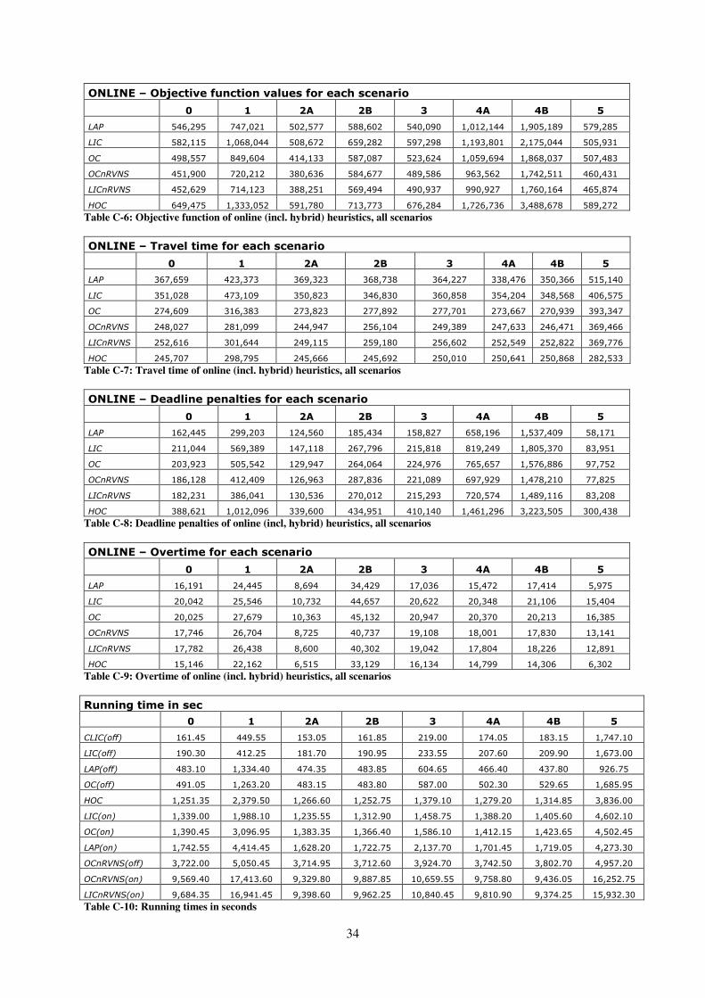
34

ONLINE – Objective function values for each scenario

0 1 2A 2B 3 4A 4B 5

LAP 546,295 747,021 502,577 588,602 540,090 1,012,144 1,905,189 579,285

LIC 582,115 1,068,044 508,672 659,282 597,298 1,193,801 2,175,044 505,931

OC 498,557 849,604 414,133 587,087 523,624 1,059,694 1,868,037 507,483

OCnRVNS 451,900 720,212 380,636 584,677 489,586 963,562 1,742,511 460,431

LICnRVNS 452,629 714,123 388,251 569,494 490,937 990,927 1,760,164 465,874

HOC 649,475 1,333,052 591,780 713,773 676,284 1,726,736 3,488,678 589,272

Table C-6: Objective function of online (incl. hybrid) heuristics, all scenarios

ONLINE – Travel time for each scenario

0 1 2A 2B 3 4A 4B 5

LAP 367,659 423,373 369,323 368,738 364,227 338,476 350,366 515,140

LIC 351,028 473,109 350,823 346,830 360,858 354,204 348,568 406,575

OC 274,609 316,383 273,823 277,892 277,701 273,667 270,939 393,347

OCnRVNS 248,027 281,099 244,947 256,104 249,389 247,633 246,471 369,466

LICnRVNS 252,616 301,644 249,115 259,180 256,602 252,549 252,822 369,776

HOC 245,707 298,795 245,666 245,692 250,010 250,641 250,868 282,533

Table C-7: Travel time of online (incl. hybrid) heuristics, all scenarios

ONLINE – Deadline penalties for each scenario

0 1 2A 2B 3 4A 4B 5

LAP 162,445 299,203 124,560 185,434 158,827 658,196 1,537,409 58,171

LIC 211,044 569,389 147,118 267,796 215,818 819,249 1,805,370 83,951

OC 203,923 505,542 129,947 264,064 224,976 765,657 1,576,886 97,752

OCnRVNS 186,128 412,409 126,963 287,836 221,089 697,929 1,478,210 77,825

LICnRVNS 182,231 386,041 130,536 270,012 215,293 720,574 1,489,116 83,208

HOC 388,621 1,012,096 339,600 434,951 410,140 1,461,296 3,223,505 300,438

Table C-8: Deadline penalties of online (incl, hybrid) heuristics, all scenarios

ONLINE – Overtime for each scenario

0 1 2A 2B 3 4A 4B 5

LAP 16,191 24,445 8,694 34,429 17,036 15,472 17,414 5,975

LIC 20,042 25,546 10,732 44,657 20,622 20,348 21,106 15,404

OC 20,025 27,679 10,363 45,132 20,947 20,370 20,213 16,385

OCnRVNS 17,746 26,704 8,725 40,737 19,108 18,001 17,830 13,141

LICnRVNS 17,782 26,438 8,600 40,302 19,042 17,804 18,226 12,891

HOC 15,146 22,162 6,515 33,129 16,134 14,799 14,306 6,302

Table C-9: Overtime of online (incl. hybrid) heuristics, all scenarios

Running time in sec

0 1 2A 2B 3 4A 4B 5

CLIC(off) 161.45 449.55 153.05 161.85 219.00 174.05 183.15 1,747.10

LIC(off) 190.30 412.25 181.70 190.95 233.55 207.60 209.90 1,673.00

LAP(off) 483.10 1,334.40 474.35 483.85 604.65 466.40 437.80 926.75

OC(off) 491.05 1,263.20 483.15 483.80 587.00 502.30 529.65 1,685.95

HOC 1,251.35 2,379.50 1,266.60 1,252.75 1,379.10 1,279.20 1,314.85 3,836.00

LIC(on) 1,339.00 1,988.10 1,235.55 1,312.90 1,458.75 1,388.20 1,405.60 4,602.10

OC(on) 1,390.45 3,096.95 1,383.35 1,366.40 1,586.10 1,412.15 1,423.65 4,502.45

LAP(on) 1,742.55 4,414.45 1,628.20 1,722.75 2,137.70 1,701.45 1,719.05 4,273.30

OCnRVNS(off) 3,722.00 5,050.45 3,714.95 3,712.60 3,924.70 3,742.50 3,802.70 4,957.20

OCnRVNS(on) 9,569.40 17,413.60 9,329.80 9,887.85 10,659.55 9,758.80 9,436.05 16,252.75

LICnRVNS(on) 9,684.35 16,941.45 9,398.60 9,962.25 10,840.45 9,810.90 9,374.25 15,932.30

Table C-10: Running times in seconds

35

Remark on Table C-10: The running time of the online heuristics depends on how long the operations

regarding a new incoming task last. For the insert operation we allowed at most two seconds and for

the possible swap operation four seconds (see Section 4.7). The post-optimization routine, used by two

of the online heuristics, was in this case restricted to the affected route and routes in close proximity

and lasted two seconds. Hence the online handling of a new task lasted at most eight seconds.

On the Impact of Real-Time Information...

Documents

Transcript of On the Impact of Real-Time Information...