On the Growth of the ServicesSector

Satya P.Das‡ and Anuradha SahaIndian Statistical Institute - Delhi Centre

Current Version: October 2011

Abstract

It aims at explaining why/how the services sector may grow faster thanmanufacturing. It develops a two-sector, closed-economy model, having amanufacturing sector and a services sector. Accumulation of human capitalserves as the basis of growth. The analysis focuses on business services,although household services are considered. It is argued that differencesin returns to scale between the two sectors and employment frictions inmanufacturing underlie how the growth rate of the services sector maybe higher. Conditions behind how within the services sector the businessservices sub-sector may grow faster than household services are identified.

JEL Classification: J24; L60; L80; O41Keywords: Business services; Household services; Manufacturing; Re-turns to scale, Employment frictions; Economic growth

‡Corresponding author: Indian Statistical Institute – Delhi Centre, 7 S.J.S.Sansanwal Marg, New Delhi 110016, India; E-mail: das@isid.ac.in

1 Introduction

To understand the growth process, the coarsest disaggregation of a macro econ-omy typically contains the industrial or the manufacturing sector, and, agricul-ture. The former is viewed as the modern sector upon which hinges the overallgrowth of the economy, while the latter is considered as the traditional, primarysector catering to the most primary need for existence – food. Starting from Lewis(1954), there are numerous two-sector models, e.g., Uzawa (1961), Matsuyama(1992) and Hayashi and Prescott (2008), among many others.

The experience of many economies in the post WWII era has become increas-ingly divorced from this traditional depiction of an economy. Over years, it is theservices sector that has overtaken manufacturing as the ‘leading’ or the largestsector of a modern economy. In many countries, it now constitutes more than50% of the GDP, and, moreover, still growing faster than manufacturing.

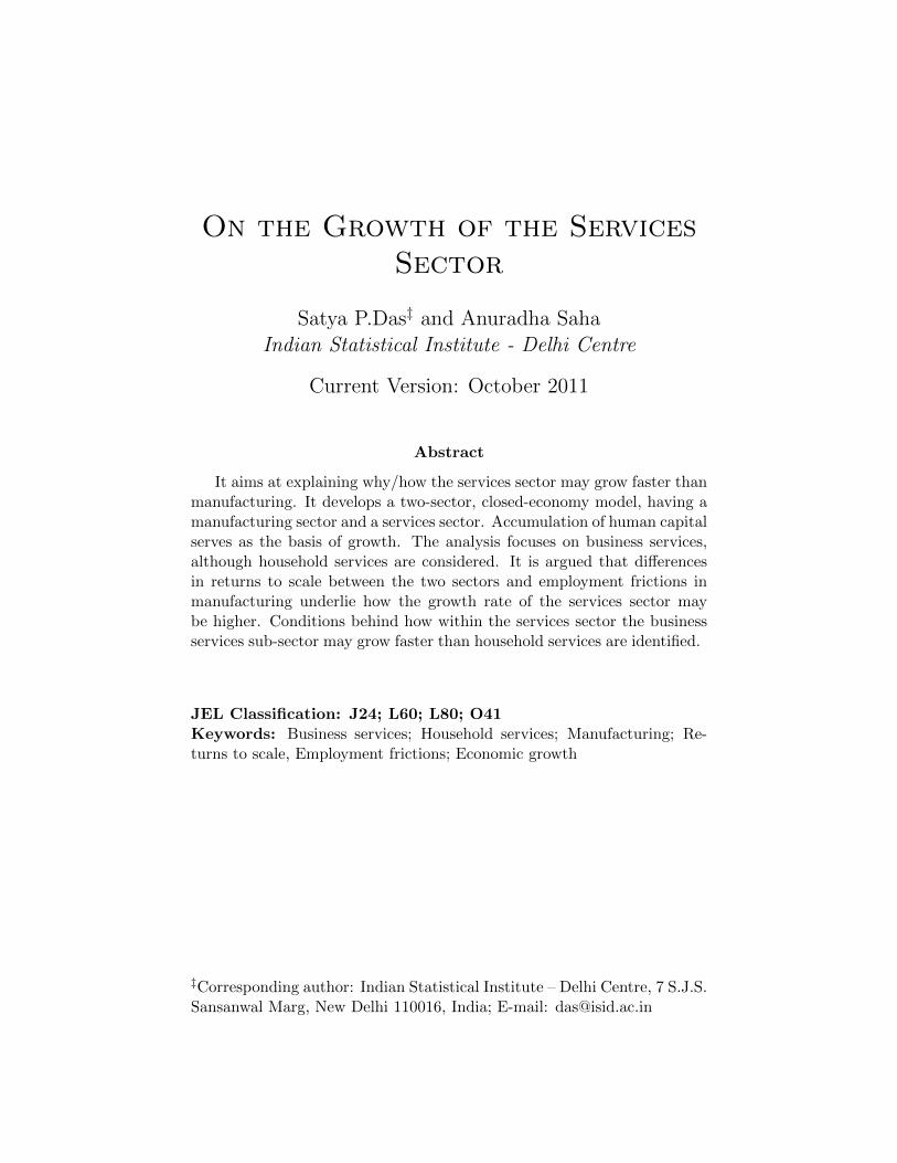
Figure 1 depicts the dynamics of sectoral composition of the economies ofU.S., U.K. and Japan into manufacturing, services and agriculture. By 1970 theservice sector constituted at least 50% of GDP of these countries and over time,its share has been growing – implying that the service sector is growing fasterthan the other two.

Table 1: Compounded Annual Growth Rates (%): Manufacturing and Services

1970-90 1990-2006 1970-2006

Country Manuf. Services Manuf. Services Manuf. ServicesUS 1.8 3.9 2.2 3.6 2.0 3.6UK -0.5 3.1 0.9 3.9 0.2 3.4

Japan 3.9 4.2 0.6 1.6 2.2 2.8Source: EU KLEMS1

Table 1 lists the annual compound growth rates of the manufacturing sectorand the services sector in the same three countries over 1970-2006. It is clearthat the latter has out-paced the former.

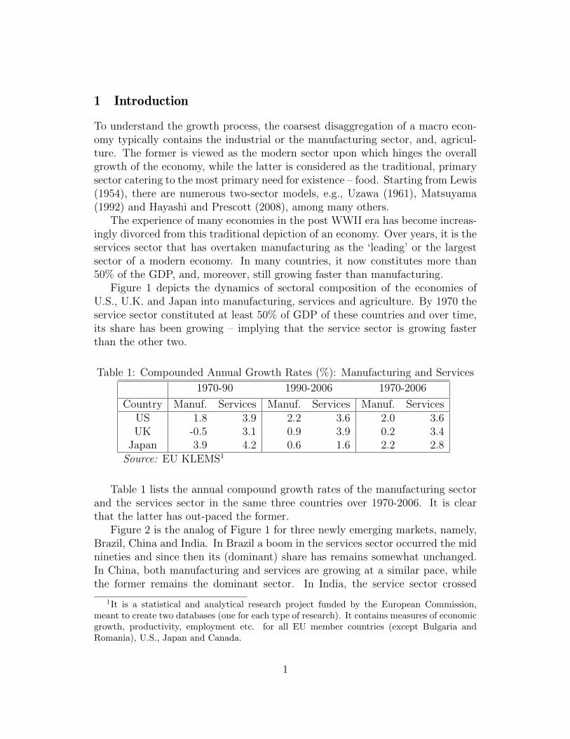
Figure 2 is the analog of Figure 1 for three newly emerging markets, namely,Brazil, China and India. In Brazil a boom in the services sector occurred the midnineties and since then its (dominant) share has remains somewhat unchanged.In China, both manufacturing and services are growing at a similar pace, whilethe former remains the dominant sector. In India, the service sector crossed

1It is a statistical and analytical research project funded by the European Commission,meant to create two databases (one for each type of research). It contains measures of economicgrowth, productivity, employment etc. for all EU member countries (except Bulgaria andRomania), U.S., Japan and Canada.

1

Figure 1: Share of Manufacturing, Services and Agriculture in real GDP: 1970-2006; Source: World Development Indicators, World Bank

2

Figure 2: Share of Manufacturing, Services and Agriculture in real GDP: 1970-2006; Source: World Development Indicators, World Bank

3

50%-share around 2000, and, has been growing faster than manufacturing andagriculture.

Buera and Kaboski (2009) emphasize that the growth of services is driven bythat of consumer services. In 2000, services formed 80% of household consump-tion in US while in the same year the services sector’s share was just over 45%in the value-added. Services in consumption have shown a slightly higher growthin the period 1950-2000 than services in value added.2

Eichengreen and Gupta (2009) present an empiricial study of the growth ofservices along with per capita income across sixty countries from 1950-2005. Theyidentify two waves of growth in this sector, one in countries with low level of percapita GDP and the second with higher levels of per capita GDP. The secondjump in the services is due to growth of services that are receptive to applicationsof information technology and are increasingly tradable across borders.

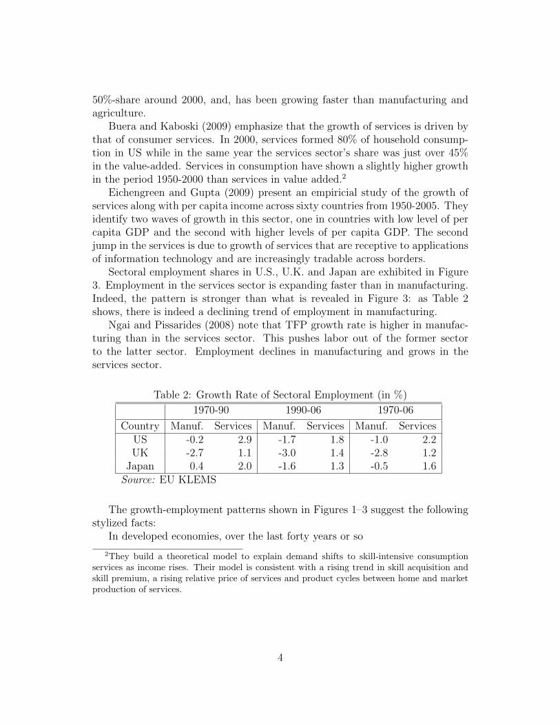
Sectoral employment shares in U.S., U.K. and Japan are exhibited in Figure3. Employment in the services sector is expanding faster than in manufacturing.Indeed, the pattern is stronger than what is revealed in Figure 3: as Table 2shows, there is indeed a declining trend of employment in manufacturing.

Ngai and Pissarides (2008) note that TFP growth rate is higher in manufac-turing than in the services sector. This pushes labor out of the former sectorto the latter sector. Employment declines in manufacturing and grows in theservices sector.

Table 2: Growth Rate of Sectoral Employment (in %)

1970-90 1990-06 1970-06

Country Manuf. Services Manuf. Services Manuf. ServicesUS -0.2 2.9 -1.7 1.8 -1.0 2.2UK -2.7 1.1 -3.0 1.4 -2.8 1.2

Japan 0.4 2.0 -1.6 1.3 -0.5 1.6Source: EU KLEMS

The growth-employment patterns shown in Figures 1–3 suggest the followingstylized facts:

In developed economies, over the last forty years or so

2They build a theoretical model to explain demand shifts to skill-intensive consumptionservices as income rises. Their model is consistent with a rising trend in skill acquisition andskill premium, a rising relative price of services and product cycles between home and marketproduction of services.

4

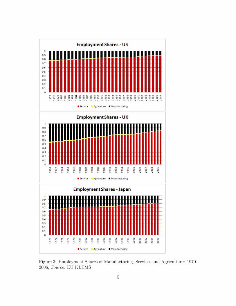
Figure 3: Employment Shares of Manufacturing, Services and Agriculture: 1970-2006; Source: EU KLEMS

5

Fact 1. The services sector has been growing faster than manufacturing.

Fact 2. Employment in the services sector has grown while that in the man-ufacturing has fallen.

Comparing the sectoral output and employment growth rates from Tables 1and 2,

Fact 3: Output growth rates exceed employment growth rates in both man-ufacturing and services.3

There are various kinds of services. National accounts of most countries haveroughly classified services into: Wholesale and Retail Trade; Hotels and Restau-rants; Transport, Storage, Post and Telecommunications; Finance, Insurance,Real Estate and Business Services; Community, Social and Personal Service; Elec-tricity, Gas and Water Supply; Construction. It is not true that all sub-sectors ofthe service sector have grown uniformly. We can broadly classify various servicesinto two types: business services and non-business (or other) services.

While non-business services constitute the lion’s share in the sector, as Figure4 illustrates, in the U.S., U.K. and Japan it is the business service sub-sectorwhich is growing faster. Table 3 records the share of this sub-sector at threepoints of time. Over the span of thirty-seven years, its share has nearly or morethan doubled in the three countries.

Table 3: Share of Business Services (% of Total Services)

Country 1970 1990 2007

US 6.65 11.27 14.77UK 8.64 12.96 17.04

Japan 4.50 9.11 13.92

Source: EU KLEMS

From Table 3, we may deduce

3That is, output per worker has increased in both sectors.

6

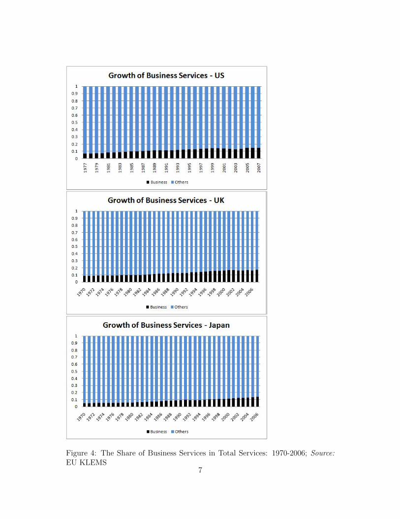
Figure 4: The Share of Business Services in Total Services: 1970-2006; Source:EU KLEMS

7

Fact 4: Business services have grown faster than non-business services.

It is worth-noting that he business services data in Table 3 and Figure 4includes outsourcing activities. Hence some critics have pointed that the growthof business services might just be an ‘accounting’ phenomenon. The tasks whichwere performed in-house by the manufacturing firms are now bought from servicefirms. However, the growth of business services does not seem to be primarilydriven by outsourcing. According to Kox and Rubalcaba (2007), outsourcing canexplain only a small part of the growth of business services. There are reasonsbehind this.

First, the IT revolution in the 1970s led to application of technology in novelways which itself led to creation of new services (such as internet, market researchand consultancy). Second, as Beyers and Lindahl (1996) have found the need forspecialized knowledge is by far the most important factor behind the demand forproducer services.4 Third, as observed by Kox (2001), the services rendered bythe business services suppliers are superior to the prior in-house service activitiesof the outsourcing firm.5

Not only the relative output and employment between manufacturing andservices sectors have been changing over time, relative price movements have alsooccurred. Figure 5 plots the trend in the price of business services and totalservices relative to manufacturing in the U.S., U.K. and Japan. Thus,

Fact 5: The price of services relative to manufacturing has been rising.

The objective of this paper is to provide a rationale behind some of the abovestylized facts.

There are a number of studies, attributing the rising share of services in GDPto preferences changes accompanying economic development. In the long run,the argument goes, the rise in real income shifts demand from agricultural goodsto manufacturing goods and then to services.6

The manufacturing sector outgrowing the agricultural sector is understand-able in terms of the preference-shift hypothesis. But the services sector outpacingmanufacturing does not seem to be adequately explained by this hypothesis, since

4This also explains why the growth of business services began post late 1960s and not before.5Raa and Wolff (2000) find that the use of business services had led to higher total factor

productivity growth in manufacturing - clearly indicating the additional benefit of businessservices over in-house services. Kox and Rubalcaba (2007) find that in Europeon Union businessservices has generated knowledge and productivity spillovers in other industries.

6See, for example, Smith (2001), Fisher (1933).

8

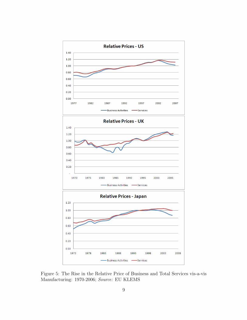
Figure 5: The Rise in the Relative Price of Business and Total Services vis-a-visManufacturing: 1970-2006; Source: EU KLEMS

9

the argument is applicable to consumer services, not business services. It is notobvious how a derived sector like business services may grow faster than the‘parent’ sector, manufacturing.

It has been argued that as a manufacturing firm grows in size it may prefernot to hire employees for menial and conventional tasks and thus outsource thesejobs to some service firms; see Goodman and Steadman (2002). The reasonbehind this has to do with labor problems associated with a large labor force,such as large scale shirking, lack of effective supervision and paperwork. BeepTechnologies, for example, quotes in its website a case of a computer chip makerhiring a staffing company to monitor and manage all of its non-exempt hiring.There is another case of a university hiring an information technology companyto manage its entire desktop, PCs and computer network. Note that a small firmor organization would have found it more economical to do these tasks in-houserather outsource them.

Even in a scenario where there are no labor ‘problems’ as such, some believethat it may be simply inefficient to employ workers than to buy the relevantservices. Quinn (2000) writes that in current times the only way of stayingahead in business is by outsourcing innovation, as innovation calls for a complexknowledge which only a broad network of specialists can offer. Leading companieshave lowered innovation costs and risks by 60 to 90 per cent while similarlydecreasing cycle times.7

The preceding argument alludes to some notions of labor congestion or frictionin the manufacturing sector.

The main purpose of this paper is to build a simple theoretical model that isindependent of the service-oriented relative demand shift, although we do considerit. Specifically, two mechanisms are explored, both hinging on the existence ofsome fundamental differences in technologies of producing manufacturing andservices.

The first assumes that returns to scale are less in manufacturing than in theservices sector. If so, it is easy to see how the latter may grow faster than theformer. Suppose that services are produced by one input, labor, and, industry-level output in the services sector is related one-to-one with labor employmentin that sector – that is, there are constant-returns in producing services at theindustry level. In contrast, let manufacturing output vary with labor and businessservices under a decreasing-returns technology. Suppose that in the steady stateemployment in both sectors grows at the same rate. It follows immediatelythat labor employment and service output would grow at the same rate, whilemanufacturing output would grow at a lesser rate. The implication is that a

7Cycle times refer to the total time it takes to complete one batch or shift of some specifiedmanufacturing and allied operations.

10

sector, namely services, whose existence is derived from demand by another, thatis, manufacturing, can grow faster.

Our second ‘story’ allows labor frictions in manufacturing, which leads tothe outcome that employment in manufacturing grows slower than that in theservices sector and therefore manufacturing grows at the lower rate.

To place this paper in its perspective, the following may be noted.

1. Our analysis abstracts from TFP changes in both manufacturing and ser-vices. Thus, the ranking of growth rates of intra-sector employment andoutput (Fact 3) is not our focus.

2. Any model to adequately explain the recent surge of the service sector musttake into account the role of IT services – particularly in the services sector.But we abstract from that, and, thus, the model is purported to providesome understanding of how and why the services sector grew faster thanmanufacturing before the advent of the IT revolution.

3. There is no denying that the service-oriented relative demand shift has con-siderable explaining power behind higher growth of the services sector as awhole. As mentioned earlier, we do incorporate it in our analysis.

The paper is organized as follows. Section 2 develops our basic model thatfeatures differences in returns to scale. There are two sectors, one producing amanufacturing good with the help of labor and business services and the otherbusiness services with the help of labor only. Employment frictions in manufac-turing are introduced in Section 3. Section 4 considers a more general technologyin the services sector, allowing for manufacturing as an input. Consumptionservices are introduced in Section 5, where it is assumed that the demand forconsumption services has unitary elasticity with respect to income. In Section6, preferences are defined such that the income elasticity of demand for servicesexceeds one, and, hence, there is a relative demand shift towards consumptionservices as income expands are examined. This section examines the ramificationsof this toward sectoral growth processes. Section 7 concludes the paper.

2 The Basic Model: Difference in Returns to Scale

The source of growth per se is not our central concern. How growth ratesmay differ across sectors is our focus. In what follows, a simple human-capital-accumulation based growth story will be developed.

We consider a closed economy having two sectors: manufacturing and ser-vices. The former produces a homogeneous good – which is the numeraire – ina perfectly competitive market. Following Eswaran and Kotwal (2002) and Mat-suyama (2010) the service-sector output is differentiated, produced in a monop-

11

olistically competitive market. Services are used as inputs in the manufacturingsector; they are not consumed by households.

The core assumption is that manufacturing is subject to diminishing-returnsto scale, while increasing returns prevail at the firm level in the services sector.More generally, higher returns to scale in the services sector – not necessarilyincreasing returns in that sector and decreasing-returns in manufacturing – wouldimply higher growth in the services sector.

Such differences in returns to scale have empirical support.There are numerous empirical studies on returns to scale in various industries,

especially in manufacturing. For the U.S. economy, Basu et al. (2006) presentreturns to scale estimates for twenty-one manufacturing industries, which areupdated from the earlier study by Basu and Fernald (1997). For manufacturing asa whole, there is evidence of decreasing returns for gross output (less so for value-added), while there are increasing returns to scale for durable manufacturingand decreasing returns of non-durable manufacturing. For Philippines, evidenceof mildly decreasing returns to scale in manufacturing is found by Yamagata(2000). For developing countries in general, Tybout (2000) reports constant ormildly increasing returns.8

Relatively fewer estimates that are available on returns to scale in the ser-vices sector indicate increasing returns. For the U.S., Basu et al. (2006) reportscale elasticities for transportation, communication, trade and a service basketincluding health, education, legal services, automotive repair, hotel business etc.,which generally exceed unity. Scale economies are also found for retail trade inIsrael (Ofer (1973)), banking and finance in the U.S. (McAllister and McManus(1993)) and hospital industry in the U.S. (Berry (1967) and Wilson and Carey(2004)).

8By using data on trade flows and factor content relations, Antweiler and Trefler (2002)estimate cost price equations and indirectly infer scale elasticities of industries in the manu-facturing sector. The methodology permits to test whether returns to scale are constant orincreasing, when the same industry is pooled across trading countries. Increasing-returns arefound in about one-third of industries in the sample, constant-returns in another one-third andfor the remaining it is inconclusive. There are no service industries in their sample.

12

2.1 The Manufacturing Sector

A manufacturing firm uses two variable inputs, labor and services, and returns toscale are diminishing. Implicitly, a fixed factor is present, which earns profits.9,10

Normalizing the fixed input to unity, let

qmt = Lαmtqβst, α, β > 0, α + β < 1, (1)

be the production function, where Lmt is labor in effective units (to be clear later)and qst is a composite of business services. At any time there are Nt varieties ofservice inputs and

qst =

(∫ Nt

0

qσ−1σ

it di

) σσ−1

, σ > 1,

where qit is the amount used of service variety i and σ is the elasticity of substi-tution between any two service inputs.

Following the adaptation by Ciccone and Matsuyama (1996) of the standardDixit-Stiglitz consumption demand system to demand for intermediates, we cal-culate the price of the composite service input - which is the price at whichthe total expenditure on all individual services equals the expenditure on thecomposite service input, i.e., pstqst =

∫ Nt0pitqitdi. The composite price has the

expression

pst =

(∫ Nt

0

p−(σ−1)it di

)− 1σ−1

. (2)

Under symmetry,qstpst = Ntqitpit. (3)

We can further use (2) to write the demand for each service input as

qit =

(pitpst

)−σqst. (4)

Profit maximization yields the standard first order conditions:

αLα−1mt q

βst = wt (5)

βLαmtqβ−1st = pst, (6)

9We may interpret the fixed factor as land. Indeed, in recent decades land has becomea major issue in manufacturing. Acquiring land for establishing or expanding manufactur-ing is getting increasingly costly and growing environmental regulations have led to stringentlimitations for the use of acquired land towards industrial activities.

10In his two-sector growth model Matsuyama (1992) also assumed decreasing returns tech-nology for manufacturing.

13

where wt is the wage rate.Labor is measured in efficiency units and it grows over time. The growth

process will be specified later, but, at the moment it is to be noted that wt is thewage rate per such efficiency unit, not earnings per worker per unit of time; see,for instance, Jung and Mercenier (2010).

2.2 The Services Sector

A service provider supplies a unique brand. The production technology of anyservice is of the simple Dixit-Stiglitz-Krugman kind that is linear and satisfiesincreasing-returns:

qit = Lit − 1,

where the fixed labor requirement has been normalized to unity. Firm i faces thedemand function (4). One obtains the standard constant-mark-up condition:

pitwt

=σ

σ − 1. (7)

Together with the zero-profit condition, the employment and output producedby each firm are fixed by technology and preference parameters:

Lit = σ; qit = qt = σ − 1. (8)

It follows that total employment as well as total output in the services sector isone to one related with the number of varieties or firms, Nt. In this sense, thissector exhibits constant-returns in the aggregate.

Further, we have

qst = Nσσ−1

t qt = Nσσ−1

t (σ − 1). (9)

Note that qst > Ntqt, implying productivity gains in manufacturing from use ofservice varieties.11

2.3 General Equilibrium

Using the last expression the manufacturing output equals

qmt = Nβσσ−1

t Lαmt(σ − 1)β. (10)

We can state the first-order condition (5) as

αqmtLmt

= wt. (11)

11See Ethier (1982), Romer (1987) and Matsuyama (2010).

14

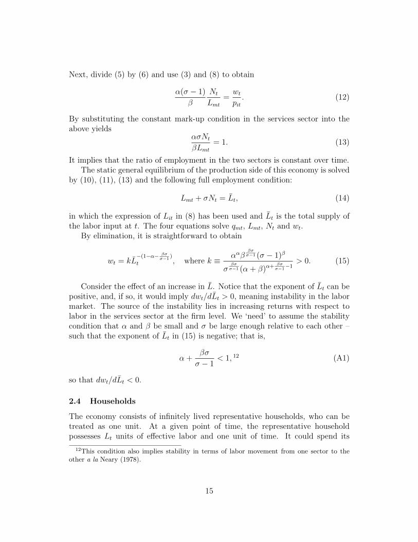
Next, divide (5) by (6) and use (3) and (8) to obtain

α(σ − 1)

β

Nt

Lmt=wtpit. (12)

By substituting the constant mark-up condition in the services sector into theabove yields

ασNt

βLmt= 1. (13)

It implies that the ratio of employment in the two sectors is constant over time.The static general equilibrium of the production side of this economy is solved

by (10), (11), (13) and the following full employment condition:

Lmt + σNt = Lt, (14)

in which the expression of Lit in (8) has been used and Lt is the total supply ofthe labor input at t. The four equations solve qmt, Lmt, Nt and wt.

By elimination, it is straightforward to obtain

wt = kL−(1−α− βσ

σ−1)

t , where k ≡ ααββσσ−1 (σ − 1)β

σβσσ−1 (α + β)α+ βσ

σ−1−1

> 0. (15)

Consider the effect of an increase in L. Notice that the exponent of Lt can bepositive, and, if so, it would imply dwt/dLt > 0, meaning instability in the labormarket. The source of the instability lies in increasing returns with respect tolabor in the services sector at the firm level. We ‘need’ to assume the stabilitycondition that α and β be small and σ be large enough relative to each other –such that the exponent of Lt in (15) is negative; that is,

α +βσ

σ − 1< 1, 12 (A1)

so that dwt/dLt < 0.

2.4 Households

The economy consists of infinitely lived representative households, who can betreated as one unit. At a given point of time, the representative householdpossesses Lt units of effective labor and one unit of time. It could spend its

12This condition also implies stability in terms of labor movement from one sector to theother a la Neary (1978).

15

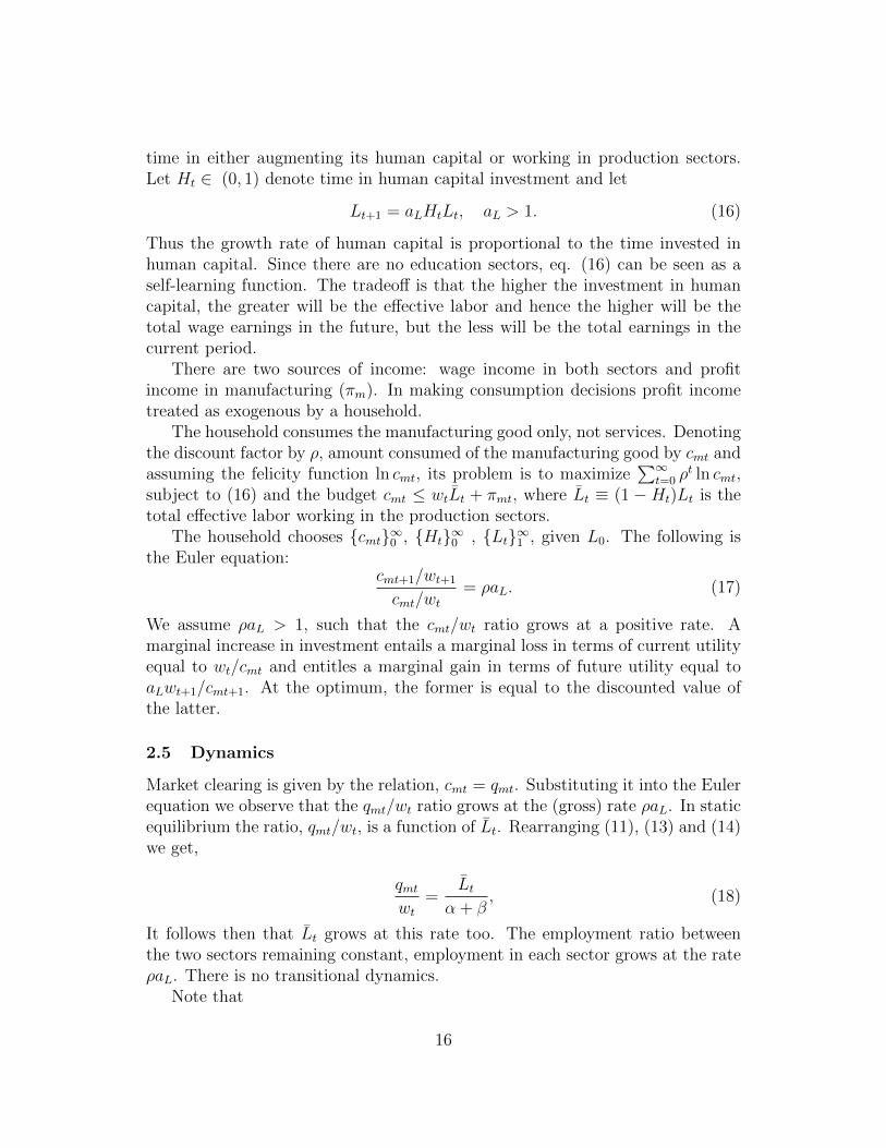
time in either augmenting its human capital or working in production sectors.Let Ht ∈ (0, 1) denote time in human capital investment and let

Lt+1 = aLHtLt, aL > 1. (16)

Thus the growth rate of human capital is proportional to the time invested inhuman capital. Since there are no education sectors, eq. (16) can be seen as aself-learning function. The tradeoff is that the higher the investment in humancapital, the greater will be the effective labor and hence the higher will be thetotal wage earnings in the future, but the less will be the total earnings in thecurrent period.

There are two sources of income: wage income in both sectors and profitincome in manufacturing (πm). In making consumption decisions profit incometreated as exogenous by a household.

The household consumes the manufacturing good only, not services. Denotingthe discount factor by ρ, amount consumed of the manufacturing good by cmt andassuming the felicity function ln cmt, its problem is to maximize

∑∞t=0 ρ

t ln cmt,subject to (16) and the budget cmt ≤ wtLt + πmt, where Lt ≡ (1 −Ht)Lt is thetotal effective labor working in the production sectors.

The household chooses cmt∞0 , Ht∞0 , Lt∞1 , given L0. The following isthe Euler equation:

cmt+1/wt+1

cmt/wt= ρaL. (17)

We assume ρaL > 1, such that the cmt/wt ratio grows at a positive rate. Amarginal increase in investment entails a marginal loss in terms of current utilityequal to wt/cmt and entitles a marginal gain in terms of future utility equal toaLwt+1/cmt+1. At the optimum, the former is equal to the discounted value ofthe latter.

2.5 Dynamics

Market clearing is given by the relation, cmt = qmt. Substituting it into the Eulerequation we observe that the qmt/wt ratio grows at the (gross) rate ρaL. In staticequilibrium the ratio, qmt/wt, is a function of Lt. Rearranging (11), (13) and (14)we get,

qmtwt

=Lt

α + β, (18)

It follows then that Lt grows at this rate too. The employment ratio betweenthe two sectors remaining constant, employment in each sector grows at the rateρaL. There is no transitional dynamics.

Note that

16

1. Essentially, the statics and the dynamics of the macro economy are disjoint.The static effects of an exogenous increase in L map one to one into whathappens over time.

2. Neither of the production sectors contributes to the basis of long-run growth– which is driven by the technology of human capital accumulation and thediscount factor.

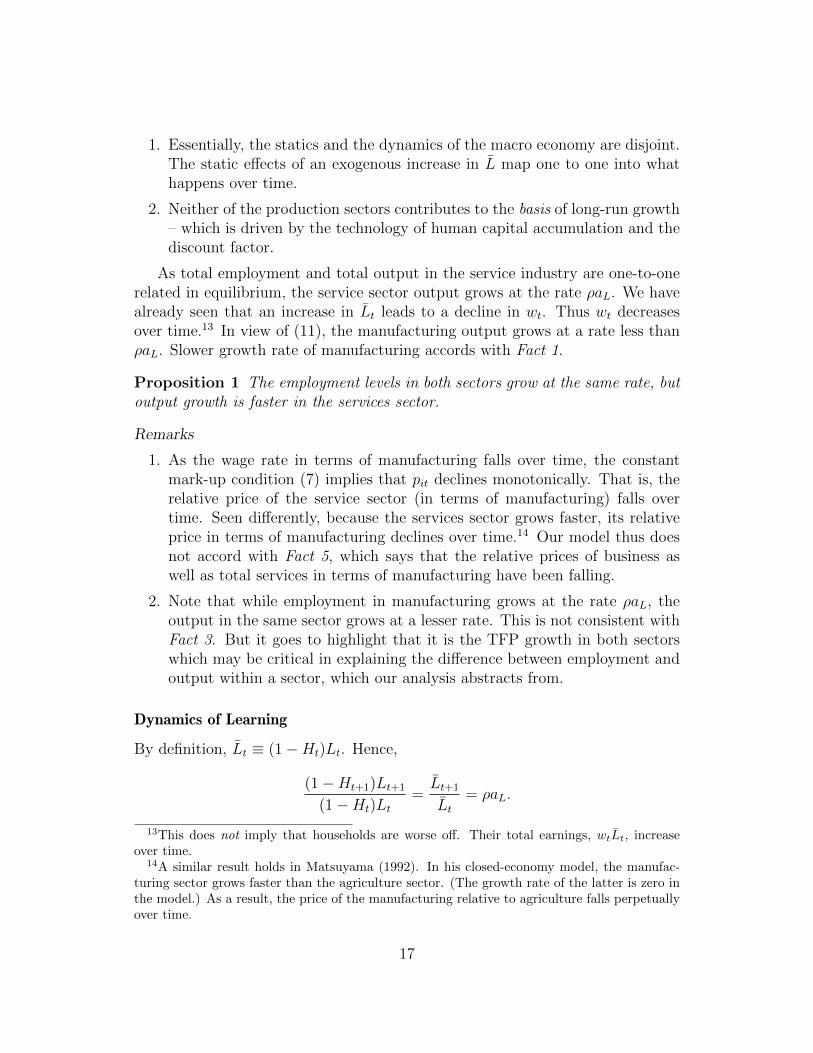
As total employment and total output in the service industry are one-to-onerelated in equilibrium, the service sector output grows at the rate ρaL. We havealready seen that an increase in Lt leads to a decline in wt. Thus wt decreasesover time.13 In view of (11), the manufacturing output grows at a rate less thanρaL. Slower growth rate of manufacturing accords with Fact 1.

Proposition 1 The employment levels in both sectors grow at the same rate, butoutput growth is faster in the services sector.

Remarks

1. As the wage rate in terms of manufacturing falls over time, the constantmark-up condition (7) implies that pit declines monotonically. That is, therelative price of the service sector (in terms of manufacturing) falls overtime. Seen differently, because the services sector grows faster, its relativeprice in terms of manufacturing declines over time.14 Our model thus doesnot accord with Fact 5, which says that the relative prices of business aswell as total services in terms of manufacturing have been falling.

2. Note that while employment in manufacturing grows at the rate ρaL, theoutput in the same sector grows at a lesser rate. This is not consistent withFact 3. But it goes to highlight that it is the TFP growth in both sectorswhich may be critical in explaining the difference between employment andoutput within a sector, which our analysis abstracts from.

Dynamics of Learning

By definition, Lt ≡ (1−Ht)Lt. Hence,

(1−Ht+1)Lt+1

(1−Ht)Lt=Lt+1

Lt= ρaL.

13This does not imply that households are worse off. Their total earnings, wtLt, increaseover time.

14A similar result holds in Matsuyama (1992). In his closed-economy model, the manufac-turing sector grows faster than the agriculture sector. (The growth rate of the latter is zero inthe model.) As a result, the price of the manufacturing relative to agriculture falls perpetuallyover time.

17

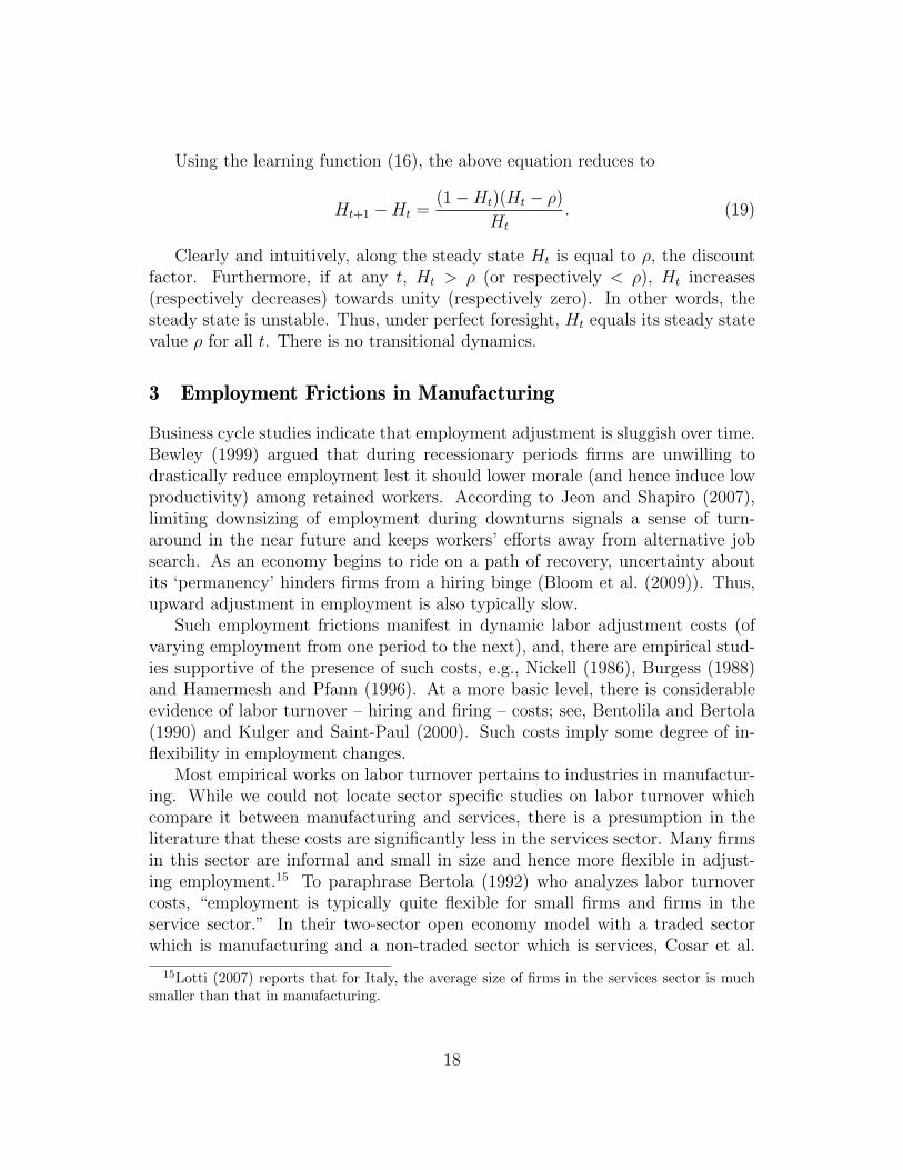
Using the learning function (16), the above equation reduces to

Ht+1 −Ht =(1−Ht)(Ht − ρ)

Ht

. (19)

Clearly and intuitively, along the steady state Ht is equal to ρ, the discountfactor. Furthermore, if at any t, Ht > ρ (or respectively < ρ), Ht increases(respectively decreases) towards unity (respectively zero). In other words, thesteady state is unstable. Thus, under perfect foresight, Ht equals its steady statevalue ρ for all t. There is no transitional dynamics.

3 Employment Frictions in Manufacturing

Business cycle studies indicate that employment adjustment is sluggish over time.Bewley (1999) argued that during recessionary periods firms are unwilling todrastically reduce employment lest it should lower morale (and hence induce lowproductivity) among retained workers. According to Jeon and Shapiro (2007),limiting downsizing of employment during downturns signals a sense of turn-around in the near future and keeps workers’ efforts away from alternative jobsearch. As an economy begins to ride on a path of recovery, uncertainty aboutits ‘permanency’ hinders firms from a hiring binge (Bloom et al. (2009)). Thus,upward adjustment in employment is also typically slow.

Such employment frictions manifest in dynamic labor adjustment costs (ofvarying employment from one period to the next), and, there are empirical stud-ies supportive of the presence of such costs, e.g., Nickell (1986), Burgess (1988)and Hamermesh and Pfann (1996). At a more basic level, there is considerableevidence of labor turnover – hiring and firing – costs; see, Bentolila and Bertola(1990) and Kulger and Saint-Paul (2000). Such costs imply some degree of in-flexibility in employment changes.

Most empirical works on labor turnover pertains to industries in manufactur-ing. While we could not locate sector specific studies on labor turnover whichcompare it between manufacturing and services, there is a presumption in theliterature that these costs are significantly less in the services sector. Many firmsin this sector are informal and small in size and hence more flexible in adjust-ing employment.15 To paraphrase Bertola (1992) who analyzes labor turnovercosts, “employment is typically quite flexible for small firms and firms in theservice sector.” In their two-sector open economy model with a traded sectorwhich is manufacturing and a non-traded sector which is services, Cosar et al.

15Lotti (2007) reports that for Italy, the average size of firms in the services sector is muchsmaller than that in manufacturing.

18

(2010) assume positive turnover costs in manufacturing, while the services sectoris assumed to be frictionless.

The objective of this section is show that employment adjustment problemsin manufacturing (relative to services) would imply higher growth rate of outputand employment in the services sector compared to manufacturing. This goes toexplain Fact 1, and, (partly) Fact 2.

However, for modeling convenience, instead of allowing for turnover costs ex-plicitly, we modify the technology of the manufacturing sector which would implyinflexibility in employment variation. That is, as output expands there is propor-tionately less employment of labor and as output declines there is proportionatelymore employment of labor.

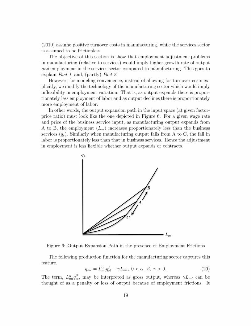
In other words, the output expansion path in the input space (at given factor-price ratio) must look like the one depicted in Figure 6. For a given wage rateand price of the business service input, as manufacturing output expands fromA to B, the employment (Lm) increases proportionately less than the businessservices (qs). Similarly when manufacturing output falls from A to C, the fall inlabor is proportionately less than that in business services. Hence the adjustmentin employment is less flexible whether output expands or contracts.

qs

Lm

A

B

C

Figure 6: Output Expansion Path in the presence of Employment Frictions

The following production function for the manufacturing sector captures thisfeature.

qmt = Lαmtqβst − γLmt, 0 < α, β, γ > 0. (20)

The term, Lαmtqβst, may be interpreted as gross output, whereas γLmt can be

thought of as a penalty or loss of output because of employment frictions. It

19

means that the output loss does not result only from loss of labor time due tofrictions (for example, there may be a loss of material property).

Furthermore, as we shall see, for the purpose of stability in the labor market,we would ‘need’ to continue with our assumption of decreasing returns to scalein manufacturing, i.e., α + β < 1.

Notice that the production function (20) is non-homothetic, while the returnsto scale are less than unity. Hence, the elasticity of input substitution is variable.Particularly, cost minimization would imply that in response to a proportionateincrease in labor and composite service input costs, the proportional reduction inlabor employment is less than that in the employment of the composite serviceinput. Likewise, in the face of a proportional decrease in input prices, labor em-ployment is increased less than proportionately compared to the service input.In this sense, γ is the measure of labor employment friction or inflexibility inmanufacturing.

Remarks

1. Specification (20) allows for negative marginal product for labor in manu-facturing – which can be interpreted as a strong congestion effect (whereasdiminishing but positive returns for any level of employment may be seenas a situation of weak congestion effect). But, profit maximization wouldimply that in equilibrium the marginal returns to labor must be positive.16

However, the possibility of negative returns has implications for equilibriumwhere the returns are positive.

2. Bruno (1968) had advocated such a production function (with the restrictionof α and β summing to unity) as belonging to a class of variable elasticityof substitution production functions. It was called the constant marginalshare production function.

The first-order condition with respect to labor now is αLα−1mt q

βst = wt+γ. The

l.h.s. is equal to the marginal product of labor in producing the gross output,while the r.h.s. can be interpreted as the effective marginal cost of labor. Thefirst-order condition with respect to the service input remains as in the basicmodel. Dividing the two first-order conditions,

αqstβLmt

=wt + γ

pst.

Unlike in the basic model, if wt and pst decline proportionately, the ratio of qst

16Interestingly, for a large public-sector conglomerate in India – SAIL (Steel Authority ofIndia Limited) – in the steel industry, Das and Sengupta (2004) found evidence of negativemarginal product of the managerial workforce.

20

to Lmt rises. This underlies why the growth rate of employment in manufacturingwill be less than that in the services sector.

Using (8), the analogs of (10), (11) and (13) are:

qmt = Nβσσ−1

t Lαmt(σ − 1)β − γLmt (21)αqmtLmt

= wt + (1− α)γ (22)

ασ

β

Nt

Lmt=wt + γ

wt. (23)

The very last equation reflects that the ratio of employment between the twosectors is not time-invariant. We may express it as

NtLitLmt

=β

α· wt + γ

wt, (23′)

which says that ratio of employment in the two sectors is proportional to theratio of effective marginal costs of hiring labor in the two sectors.

These equations along with the full-employment condition (14) characterizethe static equilibrium of the economy. By appropriate substitutions, the followingsolution equation for the wage rate is obtained:

wt + γ(wt+γwt

) βσσ−1

= α(σ − 1)β(β

ασ

) βσσ−1

(L

1 + βαwt+γwt

)−(1−α− βσσ−1

)

. (24)

Implicitly, wt = w(Lt). It is easily verified that the condition (A1) ensuresstability in the labor market, i.e., dw(Lt)/dLt < 0.

The household’s problem remains unchanged qualitatively. The Euler equa-tion is the same. Using the manufacturing market clearing condition qmt = cmt,the ratio, qmt/wt grows at the rate ρaL.

If we substitute (22) and the first-order condition (23) into the full-employmentequation (14), we have

qmtwt

=Lt

α + β

[1 +

γα(1− α− β)

αw(Lt) + β(w(Lt) + γ)

]. (25)

The r.h.s. is monotonically increasing in Lt. Hence Lt increases with qmt/wt.As the latter increases over time, Lt rises (without bound) and wt falls over time.

It is easy to establish from (21) - (23) that, under the stability condition (A1),both qmt and Lmt are negatively related to wt. Hence both grow over time. Inparticular, in view of (23), as wt decreases with time, Nt grows faster than Lmt.

21

That is, employment growth is higher in the services sector. This is main pointof this section.

Dividing (22) by (23) gives

qmtNt

=σ

β· wt[wt + (1− α)γ]

wt + γ.

The r.h.s. declines over time as the wage rate falls. Hence, qmt/Nt ratio falls,implying that the growth rate of qmt is less than that of Nt. Since the output ofthe service sector is one to one related to Nt,

Proposition 2 In the presence of employment frictions in manufacturing, thegrowth rates of output and employment in the services sector are respectivelyhigher than those of output and employment in the manufacturing sector.

Finally, we note that the dynamics of human capital investment, Ht, is dif-ferent from the basic model. It is not equal to ρ for all t. In Appendix 1 it isproved that Ht declines monotonically towards ρ.

4 Manufacturing as an Input in the Production of Services

Production of services typically uses products, tools and equipment from manu-facturing – both in the form of durable capital and intermediates. For instance,transportation services use capital goods like vehicles. Financial services exten-sively require computers and modern tools of information technology. Almostall services use a variety of “consumables” produced in the manufacturing sector.However, physical capital accumulation is beyond the scope our analysis. In whatfollows, we assume that service production requires labor, and, manufacturing asan intermediate good.

The central implication of the dependence of technology of producing serviceson manufacturing goods as inputs is a ‘locomotive’ effect: it tends to slow downthe growth rate of the services sector.

Let the production function in the services sector be extended as

qit = Lηitq′1−ηmt − 1, 0 < η < 1,

where q′mt is the manufacturing input. The following two equations are the costminimizing and the mark-up conditions (equivalently the two profit-maximizingconditions):

wt =η

1− ηq′mtLit

, (26)

pitwt

=σ

η(σ − 1)

(q′mtLit

)−(1−η)

. (27)

22

The former implies that the higher the magnitude of η, the smaller is the shareof manufacturing in the services sector. The latter implies that the mark-up isnot constant.

The zero-profit condition, together with the production function and the lasttwo equations, yields

Lηitq′1−ηmt = σ. (28)

Thus the firm-level output is time-invariant, equal to σ − 1 (as before). The lastthree equations imply

Lit =ση1−η

(1− η)1−ηw−(1−η)t (29)

pitwt

=Lit

η(σ − 1). (30)

A manufacturing firm’s problem is same as in the earlier models. For sim-plicity, we abstract from labor friction in manufacturing and thus take (1) as themanufacturing production function. Relations (10), (11) and (12) continue tohold. Substituting (30) into (12) gives

α

βη

NtLitLmt

= 1. (31)

An immediate implication is that employment in both sectors grows at the samerate.

The static general equilibrium is essentially characterized by (10), (11), (29),(31) and the full employment condition

Lmt +NtLit = L. (32)

Given Lt, these five equations determine qmt, Lmt, Nt, Lit and wt. Appendix 2proves that that condition (A1) guarantees stability in the labor market.

Once these variables are solved, eqs. (28) and (30) respectively solve q′mt andthe relative price pit. The manufacturing market clearing condition is

qmt = cmt +Ntq′mt, (33)

which essentially determines cmt.The household optimization problem remains same. The same Euler equation

results. The ratio cmt/wt grows at the rate of ρaL.We also show in Appendix 2 that effective labor supply, Lt, also grows at the

rate of ρaL. As Lt increases, (a) the wage rate falls over time, and, (b) in viewof (31), in both sectors employment grows at the same rate.17

17What is different from the case where manufacturing products are not used input in serviceproduction is that the service sector output is not one-to-one related with employment in thatsector.

23

As in the previous models, the service sector output grows faster than that ofmanufacturing sector. To see this, we substitute (29) in (31) and eliminate Lit,and then use the resulting equation to substitute for Lmt in (11). The resultantrelation is:

qmt(σ − 1)Nt

=σ

(σ − 1)βηη(1− η)1−ηwηt .

As wt falls, the ratio qmt/Nt rises, implying that the services sector grows faster.The intuition behind this finding is that falling wages make the service sectormore labor intensive over time, as seen from (26). In Appendix 2 it is derivedthat the individual sectoral growth rates are:

qmt+1

qmt= (ρaL)

1−1−α− βσ

σ−1

1−(1−η) βσσ−1

Nt+1

Nt

= (ρaL)1−

(1−η)(1−α− βσσ−1)

1−(1−η) βσσ−1 .

(34)

Observe that the growth rates of both sectors are increasing η. Hence, thesmaller the magnitude of η, i.e., the larger the share of manufacturing in theservices output, the smaller are the growth rates. Intuitively, as a slower growingsector’s output is used as input in the faster growing sector, the growth rate ofthe latter is pulled down, which, in turn, pulls down the growth rate in the formersector.

We also see that the difference between the growth rates is increasing in η. Asmaller η means a narrower gap between the growth rates.

Proposition 3 The higher the share of manufacturing in the services sector, theslower are the growth rates of both sectors and the less is the difference betweenthem.

In what follows, we revert back to the earlier scenario where labor friction ispresent in manufacturing and the manufacturing good is not used in the produc-tion of services.

5 Services for Households

While business services have been the faster growing component within the basketof services, services consumed by households hold a larger share. In this section,we introduce household or consumer services and examine the growth of themanufacturing sector vis-a-vis business services and household services.

We first consider the case of pure business and and pure consumer services– that is, services that are demanded mostly by businesses and those demanded

24

predominantly by households (such as education, personal care and health). Inother words, business and household services are different. Next we analyze thecase where same services are demanded by both businesses and households (likeretail trade, transport and communication and financial intermediation).

Unlike Buera and Kaboski (2009) however, we abstract from the trade-offbetween home and market production of consumption services and assume thatall such services are provided by the market.

5.1 Pure Household and Pure Business Services

We assume that firms in the services sector specialize in either business or house-hold services. In other words, there are two sub-sectors. The behavior of the busi-ness service providers is the same as before. Let the household service providersface similar increasing-returns linear technology. The fixed-cost component orthe variable cost coefficient (or both) may differ from those providing businessservices. For algebraic simplicity however, we use the same production function:qhit = Lhit − 1.

Households derive utility from the manufacturing good as well as consumptionservices. Let the felicity function be Ut = λ ln cmt + (1− λ) ln chst, λ ∈ (0, 1). Herechst is a composite of services demanded by the representative household and hasthe expression

chst =

(∫ Nht

0

chitσh−1

σh di

) σh

σh−1

, σh > 1, (35)

where cit is the consumption of any particular service i.The household’s problem is to maximize

∑∞t=0 ρ

tUt, subject to the learningfunction (16) and the budget cmt+phstcst ≤ wtLt+πmt, where phst is the compositeprice of consumer services.

The relation between the composite and the individual components of con-sumer services is:

phst =

(∫ Nht

0

phit−(σh−1)

di

)− 1

σh−1

. (36)

The dichotomy between the static and the dynamic components of the house-hold optimization problem is obvious. The static part yields

λ

1− λchstcmt

=1

phst, (37)

where chit = chst

(phitphst

)−σh. (38)

25

A consumer service provider faces the demand function (38) and treats chst andphst parametrically. In turn, it implies a constant mark-up first-order condition ofprofit maximization:

phitwt

=σh

σh − 1. (39)

This implies symmetry, and, together with the zero-profit condition, leads toa time-invariant level of employment and output at the firm level:

Lhit = σh; qht ≡ qhit = σh − 1. (40)

Using symmetry, the mark-up condition (39), the expressions in (40) and thatchit = qht in equilibrium, the service basket demanded by households and its pricehave the following expressions:

chst = Nht

σh

σh−1 cit = Nht

σh

σh−1 (σh − 1) (41)

phst = Nht

− 1

σh−1pit =σh

σh − 1Nht

− 1

σh−1wt. (42)

The situation of the manufacturing sector is same as in the previous model.Eqs. (21)-(23) continue to hold. Substituting (41), (42) and the manufacturinggood market clearing condition cmt = qmt into the first-order condition (37) leadsto the analog of (23) for the household sector:

λ

1− λσhNh

t

qmt=

1

wt. (43)

Finally, we have the full-employment condition:

Lmt + σNt + σhNht = Lt. (44)

It includes employment in the sub-sector producing household services.Eqs. (21)-(23) together with (43) and (44) constitute the static production

system of the economy. They determine five variables: wage, employment andoutput in manufacturing and the number of firms in the two service (sub) sectors.Appendix 3 shows that the labor market is stable under our regularity assumption(A1).

The dynamic part of the household optimization is essentially same as in thebasic model. The ratio of total household expenditure to the wage rate grows atρaL. Since the expenditure on manufacturing constitutes a constant fraction (λ)of total household expenditure, the Euler equation (17) continues to hold.

It is proved in Appendix 3 that as the ratio qmt/wt rises over time, Lt grows,wt declines and manufacturing output rises over time.

26

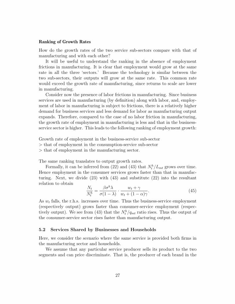
Ranking of Growth Rates

How do the growth rates of the two service sub-sectors compare with that ofmanufacturing and with each other?

It will be useful to understand the ranking in the absence of employmentfrictions in manufacturing. It is clear that employment would grow at the samerate in all the three ‘sectors.’ Because the technology is similar between thetwo sub-sectors, their outputs will grow at the same rate. This common ratewould exceed the growth rate of manufacturing, since returns to scale are lowerin manufacturing.

Consider now the presence of labor frictions in manufacturing. Since businessservices are used in manufacturing (by definition) along with labor, and, employ-ment of labor in manufacturing is subject to frictions, there is a relatively higherdemand for business services and less demand for labor as manufacturing outputexpands. Therefore, compared to the case of no labor friction in manufacturing,the growth rate of employment in manufacturing is less and that in the business-service sector is higher. This leads to the following ranking of employment growth:

Growth rate of employment in the business-service sub-sector> that of employment in the consumption-service sub-sector> that of employment in the manufacturing sector.

The same ranking translates to output growth rates.Formally, it can be inferred from (22) and (43) that Nh

t /Lmt grows over time.Hence employment in the consumer services grows faster than that in manufac-turing. Next, we divide (23) with (43) and substitute (22) into the resultantrelation to obtain

Nt

Nht

=βσhλ

σ(1− λ)· wt + γ

wt + (1− α)γ. (45)

As wt falls, the r.h.s. increases over time. Thus the business-service employment(respectively output) grows faster than consumer-service employment (respec-tively output). We see from (43) that the Nh

t /qmt ratio rises. Thus the output ofthe consumer-service sector rises faster than manufacturing output.

5.2 Services Shared by Businesses and Households

Here, we consider the scenario where the same service is provided both firms inthe manufacturing sector and households.

We assume that any particular service producer sells its product to the twosegments and can price discriminate. That is, the producer of each brand in the

27

services sector has a single production function and acts like a discriminatingmonopolist, while the market is monopolistically competitive.

The mark-up equations (7) and (39) continue to hold. Let qt and qht denotethe amount sold to manufacturing firms and households by any individual serviceprovider. The mark-up equations and the zero-profit condition imply

1

σ − 1qt +

1

σh − 1qht = 1. (46)

Hence, the equilibrium firm-level output is not time-invariant.Relations pertaining to the manufacturing sector and households are un-

changed. We bring in the variable qt into (21)-(23) and variable qht into (43),and, write them as

qmt = Lαmt(Ntqt)βN

1σ−1

t − γLmt (47)

ασ

β(σ − 1)Ntqt =

Lmt(wt + γ)

wt(48)

λσh

(1− λ)(σh − 1)Ntq

ht =

qmtwt

. (49)

The labor market clearing condition now reads as:

Nt(qt + qht + 1) + Lmt = Lt. (50)

The production side of the static general equilibrium is given by (22), thefirst-order condition with respect to labor in manufacturing, and the last fiveequations. They determine six variables: qt, q

ht , qmt, Nt, Lmt and wt. Appendix

4 shows that under the condition (A1) the labor market is stable.Since the household optimization problem is unchanged, the Euler equation

remains same and thus qmt/wt grows at the gross rate of ρaL. Appendix 4 alsoproves that as this ratio grows, L grows, the wage rate falls, and manufacturingoutput expands over time.

From (49) it follows that that consumer services grow faster than the manufac-turing output. Eqs. (22), (48) and (49) yield the following relation on intra-firmallocation of output:

qtqht

=βλ(σ − 1)σh

(1− λ)σ(σh − 1)· wt + γ

wt + γ(1− α). (51)

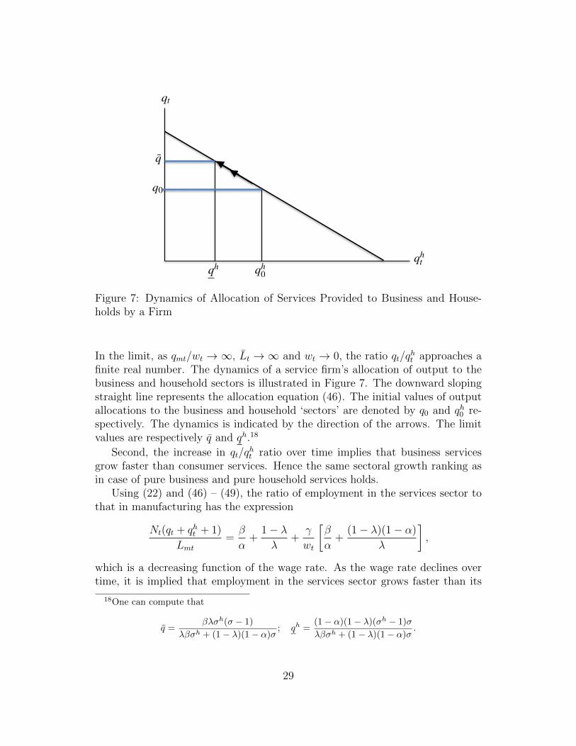
The wage rate falling over time has two implications. First, there is a substi-tution away from service provision to households towards businesses. But firmsdo not tend towards completely specializing in providing service to businesses.

28

qt

qht

q

qh

q0

qh0

Figure 7: Dynamics of Allocation of Services Provided to Business and House-holds by a Firm

In the limit, as qmt/wt →∞, Lt →∞ and wt → 0, the ratio qt/qht approaches a

finite real number. The dynamics of a service firm’s allocation of output to thebusiness and household sectors is illustrated in Figure 7. The downward slopingstraight line represents the allocation equation (46). The initial values of outputallocations to the business and household ‘sectors’ are denoted by q0 and qh0 re-spectively. The dynamics is indicated by the direction of the arrows. The limitvalues are respectively q and qh.18

Second, the increase in qt/qht ratio over time implies that business services

grow faster than consumer services. Hence the same sectoral growth ranking asin case of pure business and pure household services holds.

Using (22) and (46) – (49), the ratio of employment in the services sector tothat in manufacturing has the expression

Nt(qt + qht + 1)

Lmt=β

α+

1− λλ

+γ

wt

[β

α+

(1− λ)(1− α)

λ

],

which is a decreasing function of the wage rate. As the wage rate declines overtime, it is implied that employment in the services sector grows faster than its

18One can compute that

q =βλσh(σ − 1)

λβσh + (1− λ)(1− α)σ; qh =

(1− α)(1− λ)(σh − 1)σ

λβσh + (1− λ)(1− α)σ.

29

counterpart in manufacturing.Combining scenarios analyzed in this section and the previous section,

Proposition 4 In cases of both pure-business-cum-pure-consumption servicesand same services shared by business and households, the output of the businessservices grows faster than that of the consumer services, which, in turn, growsfaster than the manufacturing output. The growth of employment in the servicessector is higher than that in manufacturing.

Note that Proposition 4 accords with Fact 4, to the extent that consumptionservices represents non-business services.

6 Service-Oriented Relative Demand Shift

The relative rise of the service sector in the post-WWII era has been largelyattributed to the hypothesis that as real income rises the consumer demand forservices rises more than proportionately, i.e., the income elasticity of demand forhousehold services exceeds one; see, for example Eichengreen and Gupta (2009),among others.

In the presence of such a preference structure, the main implication of theensuing analysis is that, by itself, such preference shift implies not only a highergrowth rate of output in the services sector compared to manufacturing, but –less obviously so – a higher growth rate of employment in the consumer servicessector as well.

Let the household’s felicity function be

Ut = λ ln cmt + (1− λ) ln(chst + δ), λ ∈ (0, 1), δ > 0.

The presence of the parameter δ, an index of ‘non-essentiality’ of the servicesbasket in consumption, implies income elasticity of the consumer services basketto be greater than unity. Static optimization has the first-order condition

λ

1− λchst + δ

cmt=

1

phst. (52)

In the production side, we assume that business and household services aredifferent and provided by different service providers; hence the production side isthe same as in Section 5.1.

Substituting the market-clearing condition cmt = qmt as well as chst and phstfrom (41) and (42) respectively into (52) gives the analog of (43):

λ

1− λ ·σhNh

t + δσh

σh−1Nht− 1

σh−1

qmt=

1

wt. (53)

30

Earlier equations pertaining to the manufacturing sector, namely, (21) – (23),together with the full-employment condition (44), and eq. (53) solve the pro-duction side of the static general equilibrium. However, given qmt and wt, (53)implies multiple solutions of Nh

t .If preferences were homothetic, i.e. δ were zero, in view of the log-linear utility

function, the marginal utility of purchasing power (MUPP) from consuming theservices basket (the ratio of marginal utility to phst) is inversely related to totalexpenditure on it. Under symmetry, total expenditure varies directly with thenumber of varieties, Nh

t . Hence an increase in Nht would lead to a monotonic de-

cline in MUPP of services. However, with δ > 0 as an indicator of non-essentialityof services, in value terms, δphst measures how “inessential” the services basket is.The MUPP from service consumption now decreases with total expenditure onservices as well as δphst . Under symmetry, as Nh

t increases, the former increaseslinearly and MUPP tends to fall. But, since phst tends to decline with Nh

t , anincrease in Nh

t makes the services basket less inessential and MUPP tends torise. Overall, an increase in the number of varieties has a non-monotonic effecton MUPP from consuming services. This is the source of multiple solutions ofNht from eq. (53).

We express (53) as

qmtwt

= G(Nht ) ≡ λ

1− λ

[σhNh

t +δσh

(σh − 1)Nht

1

σh−1

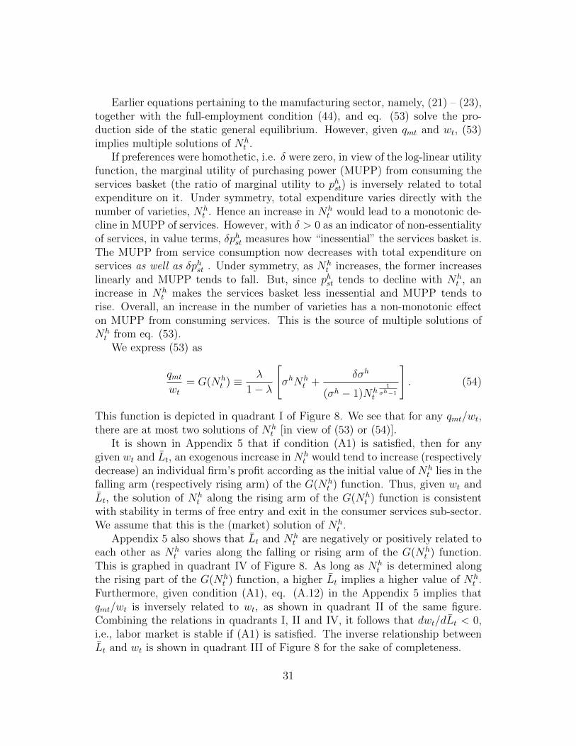
]. (54)

This function is depicted in quadrant I of Figure 8. We see that for any qmt/wt,there are at most two solutions of Nh

t [in view of (53) or (54)].It is shown in Appendix 5 that if condition (A1) is satisfied, then for any

given wt and Lt, an exogenous increase in Nht would tend to increase (respectively

decrease) an individual firm’s profit according as the initial value of Nht lies in the

falling arm (respectively rising arm) of the G(Nht ) function. Thus, given wt and

Lt, the solution of Nht along the rising arm of the G(Nh

t ) function is consistentwith stability in terms of free entry and exit in the consumer services sub-sector.We assume that this is the (market) solution of Nh

t .Appendix 5 also shows that Lt and Nh

t are negatively or positively related toeach other as Nh

t varies along the falling or rising arm of the G(Nht ) function.

This is graphed in quadrant IV of Figure 8. As long as Nht is determined along

the rising part of the G(Nht ) function, a higher Lt implies a higher value of Nh

t .Furthermore, given condition (A1), eq. (A.12) in the Appendix 5 implies thatqmt/wt is inversely related to wt, as shown in quadrant II of the same figure.Combining the relations in quadrants I, II and IV, it follows that dwt/dLt < 0,i.e., labor market is stable if (A1) is satisfied. The inverse relationship betweenLt and wt is shown in quadrant III of Figure 8 for the sake of completeness.

31

G(Nht )

Nht

S1 S2

qmt

wt

1

wt

qmtwt

III

I

Lt

IV

II

L∗

Nh∗

Figure 8: Solution of Nht and Negative Relationship Between wt and Lt

32

6.1 Dynamics

The nature of dynamic tradeoff for the household is the same. By substitutingthe first-order condition (52) into the budget constraint and eliminating chst, itcan be derived that the ratio cmt/wt grows at the rate ρaL. Hence qmt/wt alsogrows at this rate. From Figure 8, we observe that Nh

t rises and wt falls overtime.

Notice from quadrant II of Figure 8 that if wt is very high, qmt/wt is very smalland it may not intersect G(Nh

t ) in quadrant I. So for an equilibrium to exist, thewage rate should not be too high. For this to hold, we see from quadrant IIIthat Lt must exceed L∗. We presume that L0 is sufficiently large such thatL0 > L∗, and, thus Lt > L∗ for all t. The dynamics of other variables rests onthis assumption.

Output Growth Rates

The relation between the manufacturing sector and the business service firmshas not changed from the model in section 5.1. So, just as in that model thebusiness services output expands more rapidly than manufacturing output (from(22) and (23)). We observe from (53) that as long as wt falls and Nh

t rises overtime, the ratio Nh

t /qmt increases. That is, consumer services also rise faster thanmanufacturing output. Thus, both sub-sectors in the services sector grow fasterthan manufacturing. However, growth rates cannot be unambiguously rankedbetween the two sub-sectors, because, on one hand, business services tend togrow faster than consumption services due labor frictions in manufacturing, and,on the other hand, because of the relative demand shift towards consumptionservices, consumption-service production would tend to grow faster than businessservices.19

Employment Growth Rates

Because of labor frictions in manufacturing, it is obvious that employment inbusiness services grows faster than manufacturing employment. To compare con-

19Algebraically, if we divide (23) with (53) and substitute (22) into the resultant relation, weobtain

Nt

Nht

=βσhλ

σ(1− λ)· wt + γ

wt + (1− α)γ

1 +

δ

(σh − 1)Nht

σh

σh−1

.

The ranking depends on the magnitude of δ, which measures the shift in relative demandtowards consumer services. The ratio Nt/N

ht increases or decreases and thus the growth rate

of the business sub-sector exceeds or falls short of that of the consumer services sub-sector asδ is below or above a threshold.

33

sumer service sub-sector employment with manufacturing employment, we rear-range (22), (23) and (53) to get

Nht

Lmt

σh +

σhδ

σh − 1

1

Nht

σh

σh−1

=

1− λλα

[1 +

(1− α)γ

wt

]. (55)

Falling wages and rising Nht imply that employment in consumer services also

grows faster than in manufacturing sector. Notice that this ranking holds evenwhen γ = 0. The reasoning is as follows. As wt falls, it tends to lower the price ofthe composite service basket. In the presence of relative demand shift preference,the ratio of spending on consumer services to manufacturing increases, which is ademand shift effect. In both sectors, the respective household spending, equal tototal revenues, is proportional to labor costs. Hence the ratio of total labor costin the consumer services sub-sector to that in manufacturing, equal to ratio ofrespective employment levels, increases. Thus, over time as wt falls, employmentin the consumer services sub-sector grows faster than that in manufacturing.

Similar to output growth, employment growth rates in the consumer serviceand business service sub-sectors cannot be ranked however.

In summary

Proposition 5 In the presence of income-induced relative demand shift towardsconsumer services, the output growth rates as well as employment growth ratesin business and consumer services sub-sectors cannot be ranked, but both growthrates in each sub-sector exceeds those in manufacturing.

7 Concluding Remarks

In the post WWII world economy the services sector has grown consistently fasterthan manufacturing. In many countries the share of the services sector in GDPnow stands well above 50%. This phenomenon has been mainly attributed to arelative demand shift towards consuming services as real income rises. We havetaken the position that while this may be very well true it seems inadequate toexplain the growth of business services in particular.

Our analysis began with business services and consumption services were in-troduced later. We believe this has enabled us to uncover other factors (thana relative demand shift towards consumption services) behind the rise of theservices sector relative to manufacturing. One is higher returns to scale in theservices sector compared to manufacturing and the other is the prevalence ofemployment frictions in manufacturing (relative to services).

34

From the perspective of growth theory, our analysis is an example of unbal-anced growth, which has not been formally examined as intensively as balancedgrowth.

There are several stylized facts on employment and growth patterns as well asrelative price movements in the two industries. By abstracting from TFP growth,the general goal of our analysis is to understand inter-sectoral – rather than intra-sectoral – differences in the growth rates of employment and output. Factoring inTFP growth would surely enhance our understanding of growth processes acrossthe two sectors. Major productivity improvements have been recorded not just inmanufacturing but also in the services sector. The so-called Baumol’s disease (seeBaumol (1967)) has been “cured” or has not struck. (see Triplett and Bosworth(2003)).

Also, our models are unable to explain in particular the increase in the priceof services relative to manufacturing. A prevalent explanation lies in the produc-tivity increase in manufacturing compared to services; see, for example, Baumol(1967) and Alcala and Ciccone (2004) among others. Perhaps a dynamic modelincorporating some features of Matsuyama (2009), a static model which consid-ers the impact of productivity gains in manufacturing on sectoral employmentand outputs, will be useful. However, Triplett and Bosworth (2003) has notedthat the TFP growth in the services sector is no less than that in manufacturing.This seems to weaken the productivity differential argument behind the relativeprice increase of service goods. There are other explanations as well. Similar tothe current paper, Klyuev (2004) has developed a two-sector model of growth.However, the basis of growth in his model is capital accumulation. There are twomobile factors: capital and labor. The critical assumption is that manufacturingis more capital-intensive that the services sector. The Rybczinski effect impliesan increase in the relative output of the manufacturing sector at given prices. Ina closed economy it translates into an increase in the relative price of the servicessector (but a lower growth rate of the services sector). Buera and Kaboski (2009)argue that as the services sector becomes more skill intensive, the unit cost ofproviding services rises, pushing up the relative price of services. A more realisticgrowth analysis must accommodate some mechanism behind such shifts in therelative price of services.

We have incorporated a very simple source of growth, in which there is nospecific role played by either of the production sectors. The static implications ofan increase in overall resources available to an economy map directly to growthrates. It is worth exploring the implications of accumulation of physical capital,which consists of manufacturing good. To understand the so-called second waveof burgeoning share of the services sector in an aggregate economy would requirefeaturing computer capital and IT infrastructure.

Last but not least, whereas our analysis is confined to a closed economy, it is

35

important to introduce international trade – in both goods and services – whichwould permit to analyze the growth of the services sector in the context of theglobal economy.

36

Appendix 1

It refers to Section 3. We analyze the dynamics of Ht. In the presence of employ-ment frictions in manufacturing, the dynamics of Ht, human capital investment,is different from the basic model. It is not t equal to ρ for all t. It will beshown that under further restrictions Ht monotonically increases over time andapproach toward ρ.

Log differentiating (25) gives

qmtwt

= Lt[1 + Ψ(Lt)], where Ψ(Lt) ≡ −γα(1− α− β)Ltw

′(Lt)

((α + β)w(Lt) + βγ)(w(Lt) + (1− α)γ),

where the hat represents proportional change.

Using qmtwt

= ρaL − 1, the above equation can be expressed as

gLt ≡Lt+1

Lt= 1 +

ρaL − 1

1 + Ψ(Lt). (A.1)

In the basic model, γ = 0 and thus Ψ(·) was equal to zero for all t (sincew′(Lt) < 0). Here, it is positive for all t. However, as t→∞, Lt →∞. In viewof (24), both w(Lt) and Ltw

′(Lt) approach zero. Therefore, Ψ(Lt) → 0 and thegrowth rate of Lt becomes asymptotic to ρaL.

Lemma 1: Ψ is hump-shaped in Lt.

Proof: From (24) we get the inverse relationship Lt = L(wt), where L′(wt) < 0.We use it to get Ψ(Lt) ≡ G(wt). Define Ω(w) ≡ 1/G(wt). It may be checked thatΩ(·)→∞, as wt → 0 or∞. Further, Ω′′(wt) > 0. This implies that Ω(wt) is a U-shaped function in wt. Let w?t be the critical wt which minimizes Ω(·). It followsthat G(wt) attains maximum at w∗t . Since Ψ = G, Ψ(Lt) attains maximum atL(w∗t ). Thus Ψ(Lt) is hump-shaped in Lt.

We use Lt ≡ (1−Ht)Lt, the learning function (16) and (A.1) to get

∆Ht ≡ Ht+1 −Ht = (1−Ht)

(1− gLt/aL

Ht

)

= (1−Ht)

[1− 1

HtaL·(

1 +ρaL − 1

1 + Ψ(Lt)

)].

(A.2)

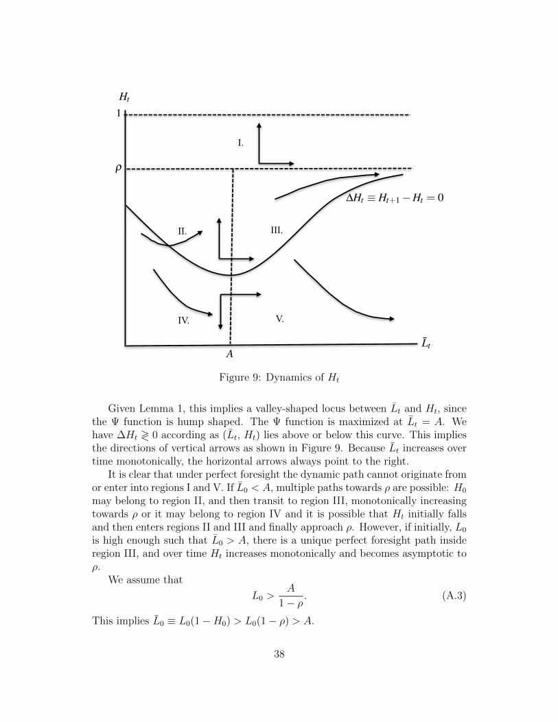
Figure 9 depicts the relation ∆Ht = 0 in the (Lt, Ht) space where Ht < 1 andLt ≥ 0. In view of (A.2), ∆Ht = 0 yields

Ht =1

aL

[1 +

ρaL − 1

1 + Ψ(Lt)

].

37

Ht

Lt

ρ

∆Ht ≡ Ht+1 −Ht = 0

I.

II. III.

IV. V.

A

1

Figure 9: Dynamics of Ht

Given Lemma 1, this implies a valley-shaped locus between Lt and Ht, sincethe Ψ function is hump shaped. The Ψ function is maximized at Lt = A. Wehave ∆Ht ≷ 0 according as (Lt, Ht) lies above or below this curve. This impliesthe directions of vertical arrows as shown in Figure 9. Because Lt increases overtime monotonically, the horizontal arrows always point to the right.

It is clear that under perfect foresight the dynamic path cannot originate fromor enter into regions I and V. If L0 < A, multiple paths towards ρ are possible: H0

may belong to region II, and then transit to region III, monotonically increasingtowards ρ or it may belong to region IV and it is possible that Ht initially fallsand then enters regions II and III and finally approach ρ. However, if initially, L0

is high enough such that L0 > A, there is a unique perfect foresight path insideregion III, and over time Ht increases monotonically and becomes asymptotic toρ.

We assume that

L0 >A

1− ρ. (A.3)

This implies L0 ≡ L0(1−H0) > L0(1− ρ) > A.

38

Under this assumption (and perfect foresight), Ht and Lt are positively re-lated, i.e., Lt ≡ Λ(Ht), where Λ′ > 0; thus

Lt =Λ(Ht)

1−Ht

.

The r.h.s. is monotonic with respect to Ht. Hence, given L0, H0 is determineduniquely.

In summary, under the assumption (A.3), Ht increases over time approachingρ, while Lt and Lt grow without bound.

Appendix 2

It refers to Section 4, which analyzes the case where the manufacturing good isused in producing services.

Stability in the Labor Market

We solve the system of equations (10), (11), (29), (31) and (32) to obtain thefollowing relationship between wage rate and labor supply

w1−(1−η) βσ

σ−1

t = a0L−(1−α− βσ

σ−1)

t (A.4)

where a0 ≡ α

(α

α + βη

)−(1−α)(βηη(1− η)1−η

(α + βη)σ

) βσσ−1

> 0.

It is readily seen in (A.4) that if the condition (A1) holds, dwt/dLt < 0, sothat the labor market is stable.

Dynamics of Lt,wt,qmt and Nt

We derive the closed form expressions of the growth rates of these variables, whichare constant over time.

The ratio of employment in the two sectors being constant (from (31)), thelabor market clearing condition (32) implies

Lmt =α

α + βηLt. (A.5)

Substituting (11), (26), (31) and (A.5) into the manufacturing market clearingcondition (33) yields

cmtwt

=1− β + βη

α + βηLt. (A.6)

39

We know from the Euler equation that cmt/wt grows at ρaL. Hence in viewof (A.4) and (A.6),

Lt+1

Lt= ρaL;

wt+1

wt= (ρaL)

−1−α− βσ

σ−1

1−(1−η) βσσ−1 .

Next, by substituting (A.6) into (A.5) and (A.4), we express Lmt and wt interms of the ratio cmt/wt. In turn, substituting those expressions into (11), weget

qmt = b0

(cmtwt

)1−1−α− βσ

σ−1

1−(1−η) βσσ−1 , where (A.7)

b0 ≡1

1− β + βη

[d0

(α + βη

1− β + βη

)−(1−α− βσσ−1)

] 1

1−(1−η) βσσ−1

> 0.

Noting again that cmt/wt grows at ρaL, (A.7) implies

qmt+1

qmt= (ρaL)

1−1−α− βσ

σ−1

1− (1−η)βσσ−1 .

Just as the growth rate of manufacturing output was calculated, we substitute(29), (A.4) and (A.6) into (31) to get,

Nt = b1

(cmtwt

)1−(1−η)(1−α− βσ

σ−1)1− (1−η)βσ

σ−1 , where (A.8)

b1 ≡βηη(1− η)1−ηc1−η

0

σ· (1− β + βη)1−η

α + βη> 0.

As output per firm is constant, the services-sector output grows at the samerate as its number of firms. (A.8) implies

Nt+1

Nt

= (ρaL)1−

(1−η)(1−α− βσσ−1)

1− (1−η)βσσ−1 .

Appendix 3

It refers to Section 5.1, which analyzes the case where business and consumptionservices are produced by different firms.

40

Stability in the Labor Market

Solving the static system of equations ((21)-(23), (43) and (44)) we obtain

h(wt) = c4L−(1−α− βσ

σ−1)t , where (A.9)

h(wt) ≡(c2 +

γc3

wt

)−(1−α− βσσ−1)

wβσσ−1

t (wt + γ)1− βσσ−1 and

c2 ≡ 1+β

α+

1− λλα

> 0; c3 ≡β

α+

(1− λ)(1− α)

λα> 0; c4 ≡ α(σ−1)β

(β

ασ

) βσσ−1

> 0.

Log-differentiating (A.9) implies dwt/dLt < 0 if (A1) is met.

Dynamics of Lt,wt,qmt and Nt

Closed form solutions of the growth rates of these variables do not exist, but wecharacterise how these variables change over time.

Eqs. (22)-(23), (43)-(44) together yield

qmtwt

=Lt

(α+β)w(Lt)+βγ

w(Lt)+(1−α)γ+ 1−λ

λ

, (A.10)

where, in view of (A.9), the wage rate is an implicit function of Lt. The r.h.s. of(A.10) is monotonically increasing in Lt. Hence qmt/wt is an increasing functionof Lt. The Euler equation implies that qmt/wt grows over time; hence Lt alsorises, and it follows from the stability of labor markets that wt declines withtime.

Substituting (A.9) into (A.10) we obtain the following relationship betweenmanufacturing output and wages:

qmt =c4

α[wt + γ(1− α)]w

−βσσ−1

1−α− βσσ−1

t (wt + γ)−

1− βσσ−1

1−α− βσσ−1 .

Log-differentiating the above, it is straightforward to derive that dqmt/dwt <0. As the wage rate falls, the manufacturing output rises over time. Further themanufacturing firm’s optimization conditions (22) and (23) imply that Nt growsand its growth rate is greater than that of qmt.

Appendix 4

This refers to Section 5.2, which examines the case where the same serviceprovider sells its services to households and businesses in the manufacturing sec-tor.

41

Stability in the Labor Market

The static system (Eqs. (22), (47)-(50)) of this economy is solved to yield

g(wt) = d3L−(1−α− βσ

σ−1)t , where (A.11)

g(wt) ≡wβt (wt + γ)1−β

(d1 + γd2

wt

) βσ−1(c2 + γc3

wt

)1−α− βσσ−1

d1 ≡β

ασ+

1− λασhλ

> 0; d2 ≡β

ασ+

(1− λ)(1− α)

ασhλ> 0; d3 ≡ α

(β(σ − 1)

ασ

)β

It can be derived that g′(wt) > 0. Hence dwt/dLt < 0 and the labor marketis stable if condition (A1) is met.

Dynamics of Lt,wt,qmt and Nt

We follow the same steps as in Appendix 3. From (A.11), implicitly, wt = w(Lt).By substituting (22) and (47)-(49) into (50) we obtain,

qmtwt

=Lt

(α+β)w(Lt)+βγ

wt(Lt)+(1−α)γ+ 1−λ

λ

.

The above expression is the exact relation which was derived in the case ofpure business and household services and is stated in (A.10). Hence as before,Lt grows over time with qmt/wt. In view of (A.11), wt falls with time.

Next, we substitute (A.11) into (A.10). It gives

qmt = w− β

1−α− βσσ−1

t (wt + γ)− 1−β

1−α− βσσ−1

(d1 +

d2

wt

) βσ−1

1−α− βσσ−1

wt + (1− α)γ

αd1−α− βσ

σ−1

3

.

The r.h.s. decreases with wt. Hence qmt increases over time. Moreover, from(22) and (23) we get that Nt grows and it grows faster than qmt.

Appendix 5

It refers to Section 6.

42

Free Entry and Exit Stability analysis in Consumer Services Sub-Sector

Substituting (22) and (23) into the manufacturing production function (21) givesqmt as a function of wt:

qm(wt) = αα(σ−1)β(β

σ

) βσσ−1

w−

βσσ−1

1−α− βσσ−1

t (wt+γ)−

1− βσσ−1

1−α− βσσ−1 [wt+(1−α)γ]. (A.12)

It can be checked that if condition (A1) holds, dqmt/dwt < 0. Hence qmt/wtdecreases with wt, as shown in quadrant II of Figure 8.

Next we substitute (41) and (42) into (52) and obtain,

qhit = qhi (wt−, Nh

t?

) ≡ 1− λλ·

σ

h − 1

σhNht

·qmt(wt

−)

wt− δ

Nht

σh

σh−1

.

Using the above expression and the price-markup condition for consumer services,the profit of a consumer service firm i can be expressed as

πhit ≡ πhit(wt−, Nh

t?

) =wtq

hi (wt, N

ht )

σh − 1− wt,

where we have used that qit = Lit − 1.Stability of entry and exit processes requires ∂πhit/∂N

ht < 0. By using Samuel-

son’s correspondence principle, we shall prove that stability is ensured if and onlyif in Figure 8, the solution of Nh

t lies in the rising part of the G(Nht ) function.

In equilibrium, πhit(wt, Nht ) = 0. Differentiating it,

dNht

dwt= − ∂πhit/∂wt

∂πhit/∂Nht

.

We know ∂πit/∂wt < 0. Hence the signs of dNht /dwt and ∂πhit/∂N

ht must be

the same. Now turn to Figure 8. If the solution of Nht is at a point such as S1

(respectively S2), dNht /dwt > (<) 0. It implies ∂πhit/∂N

ht > (<) 0 and thus free

entry-exit equilibrium is unstable (respectively stable).Therefore, stability-consistent solution of Nh

t must lie on the rising arm ofG(Nh

t ) in Figure 8.

Relationship between Lt and Nht

The system of equations describing the economy at a given point in time are(21)-(23), (44) and (53). We solve this system to get the following relationshipbetween Nh

t and Lt:

γ

[κ2Lt − f(Nh

t )

k(Nht )− Lt

+ 1

]= κ3

[κ0Lt − κ1f(Nh

t )]−(1−α) [

h(Nht )− κ1Lt

] βσσ−1

43

where

f(Nht ) ≡ σh

1− λ

[(λβ + (1− λ)(1− α))Nh

t +βλδ

(σh − 1)Nht

1

σh−1

]

h(Nht ) ≡ σh

(1− λ)(1− α− β)

[Nht +

λδ

(σh − 1)Nht

1

σh−1

]

k(Nht ) ≡ σhλ

1− λ

[Nht +

δ(α + β)(1− α)

(σh − 1)Nht

1

σh−1

]

κ0 ≡1− α

1− α− β ; κ1 ≡1

1− α− β ; κ2 ≡ 1− α; κ3 ≡ α

(β

σ

) βσσ−1

(σ − 1)β

and κ0, κ1, κ2 and κ3 are all positive. Nh∗t is the critical point at which G(Nh

t )attains minimum.

It is easy to check that when Nht ≷ Nh∗

t , f ′(Nht ) ≷ 0, h′(Nh

t ) ≷ 0 andk′(Nh

t ) ≷ 0. Hence, an increase in Lt is associated with decrease (or increase) inNht according as Nh

t < Nh∗ (or (Nht > Nh∗). This relation between Lt and Nh

t isshown in quadrant IV of Figure 8.

44

References

Alcala, Fransisco and Antonio Ciccone (2004), “Trade and Productivity,” Quar-terly Journal of Economics, Vol. 119, No. 2, pp. 613–646.

Antweiler, Werner and Daniel Trefler (2002), “Increasing Returns and All That:A View of Trade,” American Economic Review, Vol. 92, No. 1, pp. 93–119.

Basu, Susanto and John G. Fernald (1997), “Returns to Scale in U.S. Production:Estimates and Implications,” Journal of Political Economy, Vol. 105, No.2, pp. 249–283.

Basu, Susanto, John G. Fernald, and Miles Kimball (2006), “Are TechnologyImprovements Contrationary?” American Economic Review, Vol. 96, No.5, pp. 1418–1448.

Baumol, William J. (1967), “Macroeconomics of Unbalanced Growth: TheAnatomy of Urban Crises,” American Economic Review, Vol. 57, No. 3,pp. 415–426.

Bentolila, Samuel and Giuseppe Bertola (1990), “Firing Costs and Labour De-mand: How Bad is Eurosclerosis,” Review of Economic Studies, Vol. 57,No. 3, pp. 381–402.

Berry, Ralph E., Jr. (1967), “Returns to Scale in the Production of HospitalServices,” Health Services Research, Vol. 2, No. 2, pp. 123–139.

Bertola, Giuseppe (1992), “Labor Turnover Costs and Average Labor Demand,”Journal of Labor Economics, Vol. 10, pp. 389–411.

Bewley, Truman F. (1999), Why Wages Don’t Fall during a Recession, Cam-bridge, Massachusetts: Harvard University Press.

Beyers, William B. and David P. Lindahl (1996), “Explaining the Demand forProducer Services: Is Cost-Driven Externalization the Major Factor?” Pa-pers in Regional Science, Vol. 75, No. 3, pp. 351–374.

Bloom, Nicholas, Max Floetotto, and Nir Haimovich (2009), “Really Uncer-tain Business Cycles,” http://econ.duke.edu/uploads/assets/People/

Jaimoivch/BFJ_1.pdf.

Bruno, Michael (1968), “Estimation of Factor Contribution to Growth underStructural Disequilibrium,” International Economic Review, Vol. 9, pp. 49–62.

Buera, Francisco J. and Joseph P. Kaboski (2009), “The Rise of the ServiceEconomy.” NBER Working Paper No. 14822.

Burgess, Simon (1988), “Employment Adjustment in Manufacturing,” EconomicJournal, Vol. 98, No. 81-103.

45

Ciccone, Antonio and Kimoniri Matsuyama (1996), “Start Up Costs and Pe-cuniary Externalities as Barriers to Economic Development,” Journal ofDevelopment Economics, Vol. 49, pp. 33–59.

Cosar, A. Kerem, Nezih Guner, and James Tybout (2010), “Firm Dynamics, JobTurnover, and Wage Distributions in an Open Economy,” mimeo.

Das, Sanghamitra and Ramprasad Sengupta (2004), “Projection Pursuit Regres-sion and Disaggregate Productivity Effects: The Case of the Indian BlastFurnaces,” Journal of Applied Econometrics, Vol. 19, No. 3, pp. 397–418.

Eichengreen, Barry and Poonam Gupta (2009), “The Two Waves of Service Sec-tor Growth.” NBER Working Paper No. 14968.

Eswaran, Mukesh and Ashok Kotwal (2002), “The Role of the Service Sector inthe Process of Industrialization,” Journal of Development Economics, Vol.68, pp. 401–420.

Ethier, Wilfred (1982), “National and International Returns to Scale in the Mod-ern Theory of International Trade,” American Economic Review, Vol. 72,pp. 389–405.

Fisher, Allan G. B. (1933), “Capital and the Growth of Knowledge,” EconomicJournal.

Goodman, Bill and Reid Steadman (2002), “Services: Business Demand RivalsConsumer Demand in Driving Job Growth,” Monthly Labor Review, Vol.125, No. 4, pp. 3–16.

Hamermesh, Daniel S. and G.A. Pfann (1996), “Adjustment Costs in FactorDemand,” Journal of Economic Literature, Vol. 34, No. 3, pp. 1264–1292.

Hayashi, Fumio and Edward C. Prescott (2008), “The Depressing Effect of Agri-cultural Institutions on the Pre-War Japanese Economy,” Journal of Polit-ical Economy, Vol. 116, pp. 573–632.

Jeon, Don-Shin and Joel Shapiro (2007), “Downsizing and Job Insecurity,” Jour-nal of the European Economic Association, Vol. 5, No. 5, pp. 1043–1063.

Jung, Jaewon and Jean Mercenier (2010), “Routinization-Biased TechnicalChange, Globalization and Labor Market Polarization: Does Theory Fitthe Facts?”. Mimeo.

Klyuev, Vladimir (2004), “Evolution of the Relative Price of Goods and Servicesin a Neoclassical Model of Capital Accumulation.” IMF Working PaperWP/01/207.

Kox, Henk L.M. (2001), “Sources of Structural Growth in Business Ser-vices.” CPB Research Memorandum No. 12, The Hague. Available athttp://www.cpb.nl/eng/pub/cpbreeksen/memorandum/12/memo12.pdf.

46

Kox, Henk L.M. and Luis Rubalcaba (2007), “Analysing the Contribution ofBusiness Services to European Economic Growth.” MPRA Paper 2003,University Library of Munich, Germany.

Kulger, Adrianana D. and Gilles Saint-Paul (2000), “Hiring and Firiing Costs,Ad- verse Selection and Long-term Unemployment.” Working Paper, Uni-versitat Pompeu Fabra.

Lewis, Arthur (1954), “Economic Development with Unlimited Supplies of La-bor,” The Manchester School, pp. 131–199, May.

Lotti, Francesca (2007), “Firm Dynamics in Manufacturing and Services: A Bro-ken Mirror?” Industrial and Corporate Change, Vol. 16, No. 3, pp. 347–369.

Matsuyama, Kimoniri (1992), “Agricultural Productivity, Comparative Advan-tage and Economic Growth,” Journal of Economic Theory, Vol. 58, pp.317–334.

(2009), “Structural Change in an Interdependent World: A Global Viewof Manufacturing Decline,” Journal of the European Economic Association,Vol. 7, No. 2-3, pp. 478–486.

(2010), “Endogenous Ranking and Equilibrium Lorenz Curve Across (ex-ante) Identical Countries.” mimeo.

McAllister, Patrick H. and Douglas McManus (1993), “Resolving the Scale Effi-ciency Puzzle in Banking,” Journal of Banking and Finance, Vol. 17, No.2-3, pp. 389–405.

Neary, J. Peter (1978), “Dynamic Stability and Factor Market Distortions,”American Economic Review, Vol. 68, No. 4, pp. 671–682.

Ngai, L. Rachel and Christopher A. Pissarides (2008), “Trends in Hours andEconomic Growth,” Review of Economic Dynamics, Vol. 11, No. 2, pp.239–256.

Nickell, Stephen (1986), “Dynamic Models of Labor Demand,” in Orley Ashen-felter and R. Leyard eds. Handbook of Labor Economics, Volume I.

Ofer, Gur (1973), “Returns to Scale,” Retail Trade, Vol. 19, No. 4, pp. 363–384.

Quinn, James B. (2000), “Outsourcing Innovation: The New Engine of Growth,”Sloan Management Review, Vol. 41, No. 4, pp. 13–28.

Raa, Thijs ten and Edward N. Wolff (2000), “Outsourcing of Services and the Pro-ductivity Recovery in U.S. Manufacturing in the 1980s and 1990s,” Journalof Productivity Analysis, Vol. 16, No. 2, pp. 149–165.

Romer, Paul (1987), “Growth Based Increasing Retusn due to Specialization,”American Economic Review, Vol. 77, pp. 56–62.

47

Smith, Adam. (Edited by C. J. Bullock) (2001), Wealth of Nations. Vol. X. TheHarvard Classics, New York: P.F. Collier and Son, 1909–14.

Triplett, Jack E. and Barry P. Bosworth (2003), “Productivity MeasurementIssues in Services Industries: “Baumol’s Disease” Has Been Cured,” NewYork FED Economic Policy Review, Vol. 9, pp. 23–33.

Tybout, James (2000), “Manufacturing Firms in Developing Countries: How WellDo They Do, and Why?” Journal of Economic Literature, Vol. 38, No. 1,pp. 11–44.

Uzawa, Hirofumi (1961), “On a Two-Sector Model of Economic Growth,” Reviewof Economic Studies, Vol. 29, No. 1, pp. 40–47.

Wilson, Paul and Kathleen Carey (2004), “Nonparametric Analysis of Returnsto Scale in the U.S. Hospital Industry,” Journal of Applied Econometrics,Vol. 19, No. 4, pp. 505–524.

Yamagata, Tatsufumi (2000), “Procyclical Productivity and Returns-to-Scale inPhilippine Manufacturing,” Asian Economic Journal, Vol. 14, pp. 389–414.

48