Acta Appl Math manuscript No.(will be inserted by the editor)

On the Geometry of Point-Plane Constraints on Rigid-BodyDisplacements

J.M. Selig

Received: date / Accepted: date

Abstract In this paper the rigid-body displacements that transform apoint in such a waythat it remains on a particular plane are studied. These setsof rigid displacements are re-ferred to as point-plane constraints and are given by the intersection of the Study quadricof all rigid displacements with another quadric in 7-dimensional projective space. The setof all possible point-plane constraints comprise a Segre variety. Two different classes ofproblems are investigated. First instantaneous kinematics, for a given rigid motion there arepoints in space which, at some instant, have no torsion or have no curvature to some order.The dimension and degrees of these varieties are found by very simple computations. Thecorresponding problems for point-sphere constraints are also found. The second class ofproblems concern the intersections of several given constraints. Again the characteristics ofthese varieties for different numbers of constraints are found using very simple techniques.

Keywords Rigid-body displacements· constraints· instantaneous kinematics· homology

PACS 70B10· 53A17 · 14N25

1 Introduction

This work is concerned with constraints on the displacements of a rigid body. In particu-lar with constraints that require a point in the body to remain in a fixed plane. However,constraints where a point is required to remain on a fixed sphere will be briefly consideredtoo. These will be called point-plane or point-sphere constraints respectively. Wampler [10]argued that the point-plane constraints arise in many area of kinematics and robotics. Asexamples he cites the kinematics of certain linkages, problems in metrology concerned withlocating the position and orientation of a rigid body and also problems in robot vision wherefeature points are restricted to certain lines.

To these problems another is contributed here: instantaneous kinematics. The previousproblems all reduce to finding the intersection of several given point-plane constraints. That

J.M. SeligLondon South Bank University, London, U.K.Tel.: +(0)20-7815-7461E-mail: seligjm@lsbu.ac.uk

2 J.M. Selig

is the rigid-body displacements which satisfy all the constraints. For instantaneous kine-matics the problem is, in a sense, dual to this problem. Here the motion is given and thepoints which remain on some plane or sphere are sought. Theseproblems can be answeredby studying the spaces of all possible point-plane or point-sphere constraints.

Most of the examples considered in this work are not new and insome cases date back tothe late 19th century. However, the methods used in this workare novel, at least in kinemat-ics and robotics. The techniques used come from algebraic geometry, in particular homologyis used as a generalisation of degree and Bezout’s theorem to varieties such as quadrics andproducts of projective spaces. An excellent introduction to these methods is [3]. In otherwork, for example see [5], much more advanced methods from algebraic geometry are used.The idea here is to keep the use of advanced techniques to a bare minimum. This is partlyto show how far we can get with ideas that are only a little moreadvanced than those com-monly used. The main motivation though, is to show that thesemethods are simple to useand provide useful new information about important problems in robotics and mechanismstheory.

In a previous work [8], a particular Clifford algebra was used to compare point-plane,point-sphere and some other geometric constraints. The present work concentrates on thegeometry of the constraints so dual quaternions are used here to reprove that point-planeand point-sphere constraints are represented by the intersection of the Study quadric withanother quadric hypersurface inP7. The following section gives a brief introduction to theStudy quadric and dual quaternions.

2 Dual Quaternions and the Study quadric

A dual quaternion is an element of the algebraH⊗D, the tensor product of the quaternionswith the ring of dual numbers. A typical dual quaternion has the form,a+ εc wherea andc are quaternions andε is the dual unit which commutes with scalars and quaternionsandsquares to zero,ε2 = 0. The quaternions have the form,

a= a0+a1i +a2 j +a3k

wherei, j andk are quaternion generators which satisfyi2 = j2 = k2 = −1, i j = k, jk = i,ki = j and so on.

It is well known that rotations can be represented by unit quaternions. A unit quaternionr = a0+a1i +a2 j +a3k, satisfies the equation,rr− = 1 that isa2

0+a21+a2

2+a23 = 1, since

the quaternion conjugate is given byr− = a0−a1i −a2 j −a3k. If p= xi+y j+zk is a purequaternion representing a point in space, then a rotation isgiven by a product of the form,

p′ = rpr−.

Both r and−r give the same rotation so the unit quaternions represent a double cover of thegroup of rotations about the origin.

To represent rigid displacements the dual numbers are introduced. Now a point in spaceis represented by a dual quaternion of the form 1+ ε p, with p as above. Rotations arerepresented by unit quaternions again but translations arerepresented by dual quaternionsof the form 1+(1/2)ε(txi + ty j + tzk). In this representationtx, ty andtz are the componentsof the translation vector. A general dual quaternion acts onpoints in space according to therelation,

1+ ε p′ = (a+ εc)(1+ ε p)(a−− εc−).

On the Geometry of Point-Plane Constraints on Rigid-Body Displacements 3

Notice, that both(a+ εc) and−(a+ εc) give the same rigid displacement. Not every dualquaternion represents a rigid displacement, first it must satisfy aa− = 1 that is,

a20+a2

1+a22+a2

3 = 1. (1)

Second it must satisfyac−+ca− = 0, to see this observe thatt = (1/2)ca− and sincet hasno scalar partt + t− = 0. In coordinates this equation becomes,

a0c0+a1c1+a2c2+a3c3 = 0. (2)

To get rid of the double valued nature of this representation(a0 : a1 : a2 : a3 : c0 : c1 : c2 : c3)are taken as homogeneous coordinates inP

7. Points inP7 are rays through the origin inR8

(in the following the scalars will often implicitly be assumed to be complex rather than realto make degree computations simpler). Almost all of these rays will meet the affine quadricgiven by (1) in the two points representing the same rotation. So only the second equation (2)is relevant. This is a homogeneous quadratic equation, the solution to this equation form asix-dimensional quadric inP7 known as the Study quadric. Almost all points of this quadricare in one-to-one correspondence with the group of proper rigid-body displacements, that isthe Lie groupSE(3). The exceptions to this correspondence consist of a single 3-plane ofelements satisfyinga0 = a1 = a2 = a3 = 0. This 3-plane of ‘ideal element’ or ‘elements atinfinity’ will be referred to asA∞ in the following.

More details on these ideas can be found in [7].

3 Quadratic Constraints

3.1 A Point on a Plane

The standard vector equation for a pointp to lie on a plane with normal vectorn is,

n ·p = δ

whereδ is a real constant. If the point lies on the plane initially then it remains on the planeafter a rigid displacement if,

n · (Rp+ t−p) = 0,

where as usual,R is a 3×3 rotation matrix andt a translation vector.

Proposition 1 The rigid body displacements which preserve the incidence of a point with aplane comprise an open set of a quadric hypersurface inP

7.

Proof In the quaternion representation introduced above, the effect of a rotation can bewritten apa− and the pure quaternion representing a translation is 2ca− or −2ac−. Nowusing the fact thataa− = 1, the equation for the plane can be written,

n(apa−− paa−+2ca−)−+(apa−− paa−+2ca−)n− = 0

or more compactly as,Re(

(apa−− paa−+2ca−)n−)

= 0

where Re() denotes the real (scalar) part of the quaternion. Notice that given a pointp anda normaln this equation is quadratic in the components of the dual quaterniona+ εc. ⊓⊔

4 J.M. Selig

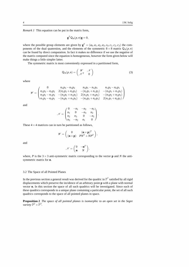
Remark 1This equation can be put in the matrix form,

gTQπ(p,n)g= 0,

where the possible group elements are given bygT = (a0,a1,a2,a3,c0,c1,c2,c3) the com-ponents of the dual quaternion, and the elements of the symmetric 8× 8 matrixQπ(p,n)can be found by direct computation. In fact it makes no difference if we use the negative ofthe matrix computed since the equation is homogeneous, however the form given below willmake things a little simpler latter.

The symmetric matrix is most conveniently expressed in a partitioned form,

Qπ(p,n) =

(

W N

N T 0

)

(3)

where

W =

0 n2p3−n3p2 n3p1−n1p3 n1p2−n2p1

n2p3−n3p2 2(n2p2+n3p3) −(n2p1+n1p2) −(n3p1+n1p3)n3p1−n1p3 −(n2p1+n1p2) 2(n1p1+n3p3) −(n3p2+n2p3)n1p2−n2p1 −(n3p1+n1p3) −(n3p2+n2p3) 2(n1p1+n2p2)

and

N =

0 −n1 −n2 −n3

n1 0 −n3 n2

n2 n3 0 −n1

n3 −n2 n1 0

.

These 4×4 matrices can in turn be partitioned as follows,

W =

(

0 (n×p)T

(n×p) PNT +NPT

)

,

and

N =

(

0 −nT

n N

)

.

where,P is the 3×3 anti-symmetric matrix corresponding to the vectorp andN the anti-symmetric matrix forn.

3.2 The Space of all Pointed Planes

In the previous section a general result was derived for the quadric inP7 satisfied by all rigiddisplacements which preserve the incidence of an arbitrarypointp with a plane with normalvectorn. In this section the space of all such quadrics will be investigated. Since each ofthese quadrics corresponds to a unique plane containing a particular point, the set of all suchquadrics corresponds to the space of all pointed planes in space.

Proposition 2 The space of all pointed planes is isomorphic to an open set inthe SegrevarietyP2×P

3.

On the Geometry of Point-Plane Constraints on Rigid-Body Displacements 5

Proof Suppose,n = (n1,n2,n3)T is the normal to the plane, clearly multiplying this vector

by a non-zero scalar will not affect the solutions of the quadratic equation determined by aquadric. Also the components ofn cannot all be zero, so we can assume that the components(n1 : n2 : n3) are homogeneous coordinates for a 2-dimensional projective spaceP2. Next wecan assume that the components of the point are given byp= (p1, p2, p3)

T . Let us introduceanother quantityp0 and use this to multiply the top right and bottom left blocks of Qπ(p,n),see (3). Now the components(p0 : p1 : p2 : p3) can be taken as homogeneous coordinatesin aP3. This does however introduce a set of ideal pointed planes, the set of quadrics withp0 = 0. The elements of the matrixQπ(p,n) are now linear combinations of elements ofthe form pin j with 0 ≤ i ≤ 3 and 1≤ j ≤ 3. Clearly, there are 12 different such elementsand among the components ofQπ(p,n) can be found 12 linearly independent combinations.The twelve elementspin j can be thought of as homogeneous coordinates in aP

11 but notall points in this projective space correspond to pointed planes, only those with coordinateswhich can be decomposed into products ofpis with n js. This is a well known constructionin algebraic geometry known as a Segre variety. It is the image ofP2×P

3 in P11. ⊓⊔

This Segre variety is five dimensional and has degree(2+3

2

)

= 10, see [3,§18.15]. Alsoaccording to Harris [3,§9.21], the lines in this Segre variety form two families, onefamilyare the images of lines inP2 and the other family come from lines inP3.

Corollary 1 Lines in the Segre varietyP2 ×P3 correspond to pencils of quadrics which

either represent pointed lines or points on parallel planes.

Proof Consider the intersection of two quadricsQπ(p,n1) andQπ(p,n2). The intersectionwill consist of displacements which preserve the incidenceof the pointp with two differentplanes with normalsn1 andn2, in other words the set of displacement which leave the pointon a line. The line being the intersection of the planes. Fromthe structure of the matricesgiven in (3) above, it is clear that,

λQπ(p,n1)+µQπ(p,n2) =Qπ(p,λn1+µn2),

for arbitrary scalarsλ , µ. That is the linear system of quadrics determined by the two origi-nal quadric lies entirely in the Segre variety. Another way of putting this is that the pencil ofquadrics determined by a point on a line in space is given by a line in the Segre variety. Thisis not the case for two general quadricsQπ(p1,n1) andQπ(p2,n2), the pencil determinedby these quadrics will be a line inP11. However, it is also easy to see that for a pair of pointsrestricted to parallel planes the line again lies in the Segre variety. ⊓⊔

Remark 2Finally here it is not hard to see that the set of displacements which lie in theintersection of three quadrics determined by three non-collinear points restricted to parallelplanes actually form a subgroup of the group of rigid-body displacements. This subgroupis isomorphic to the group of proper planar rigid displacements: SE(2) if two or all threeplanes are different. If all three parallel planes coincidethen reflections in lines lying in theplane are also allowed, so the relevant subgroup isE(2) in these cases.

3.3 A Point on a Sphere

For a pointp to lie on a sphere with centreq and radiusr the equations is,

(p−q) · (p−q) = r2.

6 J.M. Selig

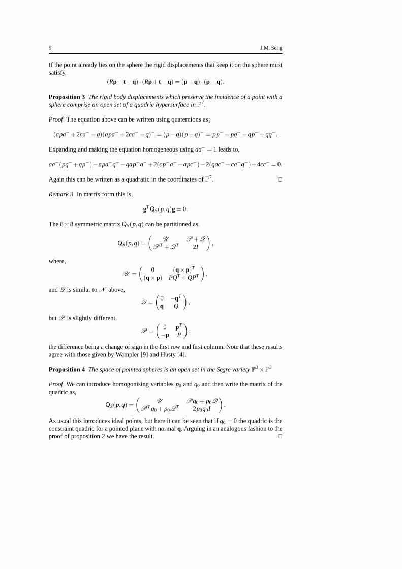
If the point already lies on the sphere the rigid displacements that keep it on the sphere mustsatisfy,

(Rp+ t−q) · (Rp+ t−q) = (p−q) · (p−q).

Proposition 3 The rigid body displacements which preserve the incidence of a point with asphere comprise an open set of a quadric hypersurface inP

7.

Proof The equation above can be written using quaternions as¡

(apa−+2ca−−q)(apa−+2ca−−q)− = (p−q)(p−q)− = pp−− pq−−qp−+qq−.

Expanding and making the equation homogeneous usingaa− = 1 leads to,

aa−(pq−+qp−)−apa−q−−qap−a−+2(cp−a−+apc−)−2(qac−+ca−q−)+4cc− = 0.

Again this can be written as a quadratic in the coordinates ofP7. ⊓⊔

Remark 3In matrix form this is,

gTQS(p,q)g= 0.

The 8×8 symmetric matrixQS(p,q) can be partitioned as,

QS(p,q) =

(

U P +Q

PT +QT 2I

)

,

where,

U =

(

0 (q×p)T

(q×p) PQT +QPT

)

,

andQ is similar toN above,

Q =

(

0 −qT

q Q

)

,

but P is slightly different,

P =

(

0 pT

−p P

)

,

the difference being a change of sign in the first row and first column. Note that these resultsagree with those given by Wampler [9] and Husty [4].

Proposition 4 The space of pointed spheres is an open set in the Segre variety P3×P3

Proof We can introduce homogonising variablesp0 andq0 and then write the matrix of thequadric as,

QS(p,q) =

(

U Pq0+ p0Q

PTq0+ p0QT 2p0q0I

)

.

As usual this introduces ideal points, but here it can be seenthat if q0 = 0 the quadric is theconstraint quadric for a pointed plane with normalq. Arguing in an analogous fashion to theproof of proposition 2 we have the result. ⊓⊔

On the Geometry of Point-Plane Constraints on Rigid-Body Displacements 7

4 Infinitesimal Kinematics

The results of this section are classical, many of them seem to be due to Schonflies [6]. Thenovelty here is the simplicity of the proofs which depend on propositions 2 and 4 above.

Corollary 2 There are, in general, 10 points which in 6 positions lie in a plane.

Proof The six positions refer to positions of a rigid body. These can be thought of as ahome position and five rigid displacementsg1, g2, g3, g4, g5. These displacements will movethe home position to one of the five other positions. On the other hand we might considersuccessive displacements from one position to the next; such displacements would be givenby g1, g2g−1

1 , g3g−12 , . . . ,g5g−1

4 . In either case, we may consider the points which remainon a plane after a particular displacement. These points andplanes are determined by thequadrics. If,

gTi Qπ(p,n)gi = 0,

then the quadricQπ(p,n) represents a point on a plane which remains on the plane afterthe displacementgi . Notice that this equation is linear in the elements of the symmetricmatrix Qπ(p,n), hence such an equation determines a hyperplane in theP

11 of homoge-neous coordinatespin j . The intersection of five such hyperplanes will, in general be a six-dimensional plane inP11. Since the Segre variety is 5 dimensional, the intersectionwith asix-dimensional plane will give a finite number of points. Ten intersections in general, sincethe degree of the Segre variety is 10. ⊓⊔

Results on finite numbers of positions were originally intended to produce results aboutinfinitesimal motion after a suitable limiting process. These problems are considered next.

4.1 Contact with Planes

Let g(t) be an analytic rigid-body motion. The Taylor expansion of the motion about thepoint g(0) = g0 is given by,

g(t) = g0+dg0

dtt +

d2g0

dt2t2

2+

d3g0

dt3t3

3!+ · · · .

The corresponding Lie algebra elements is given bys= (dg/dt)g−1 and so the first fewderivatives can be written,

dgdt

= sg,d2gdt2

= (s+s2)g,d3gdt3

= (s+2ss+ss+s3)g, . . . .

The Lie algebra elements and its derivatives are to be treated as dual quaternions in theabove. We can choose the coordinate frame so thatg(0) = 1, the identity in the group, thiswill not affect the results here. Expressions will be simplified if we set,

z0 = 1, z1 = s, z2 = (s+s2), z3 = (s+2ss+ss+s3), . . . .

The Taylor expansion can then be written as,

g(t) = z0+z1t +z2t2

2+z3

t3

3!+ · · · .

8 J.M. Selig

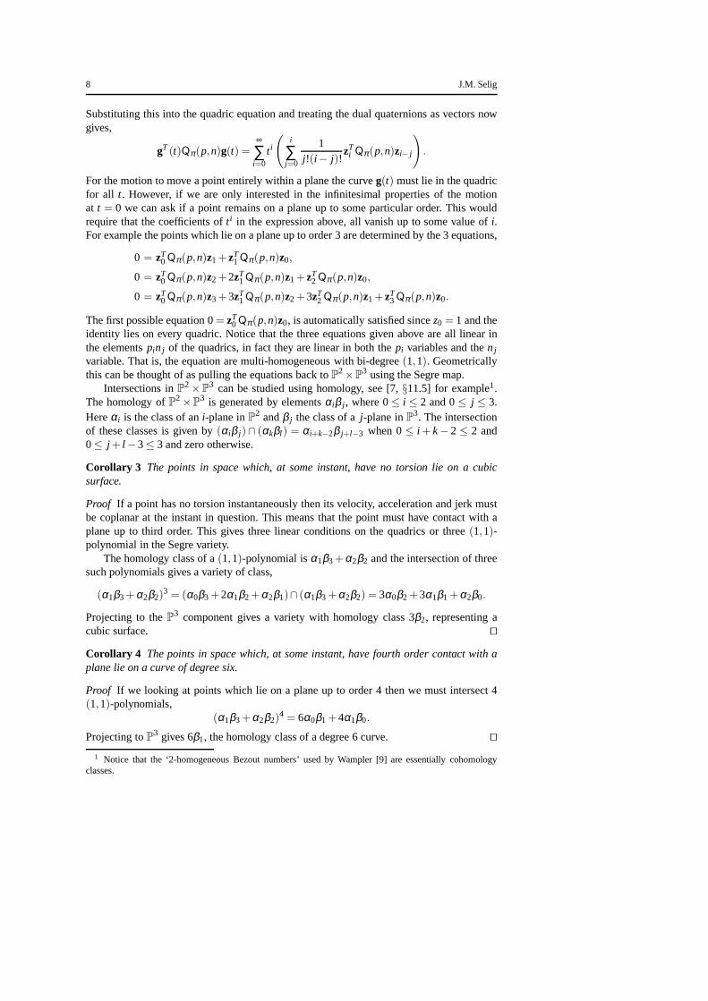
Substituting this into the quadric equation and treating the dual quaternions as vectors nowgives,

gT (t)Qπ(p,n)g(t) =∞

∑i=0

t i

(

i

∑j=0

1j!(i − j)!

zTi Qπ(p,n)zi− j

)

.

For the motion to move a point entirely within a plane the curve g(t) must lie in the quadricfor all t. However, if we are only interested in the infinitesimal properties of the motionat t = 0 we can ask if a point remains on a plane up to some particular order. This wouldrequire that the coefficients oft i in the expression above, all vanish up to some value ofi.For example the points which lie on a plane up to order 3 are determined by the 3 equations,

0 = zT0Qπ(p,n)z1+zT

1Qπ(p,n)z0,

0 = zT0Qπ(p,n)z2+2zT

1Qπ(p,n)z1+zT2Qπ(p,n)z0,

0 = zT0Qπ(p,n)z3+3zT

1Qπ(p,n)z2+3zT2Qπ(p,n)z1+zT

3Qπ(p,n)z0.

The first possible equation 0= zT0Qπ(p,n)z0, is automatically satisfied sincez0 = 1 and the

identity lies on every quadric. Notice that the three equations given above are all linear inthe elementspin j of the quadrics, in fact they are linear in both thepi variables and then j

variable. That is, the equation are multi-homogeneous withbi-degree(1,1). Geometricallythis can be thought of as pulling the equations back toP

2×P3 using the Segre map.

Intersections inP2 ×P3 can be studied using homology, see [7,§11.5] for example1.

The homology ofP2×P3 is generated by elementsαiβ j , where 0≤ i ≤ 2 and 0≤ j ≤ 3.

Hereαi is the class of ani-plane inP2 andβ j the class of aj-plane inP3. The intersectionof these classes is given by(αiβ j)∩ (αkβl ) = αi+k−2β j+l−3 when 0≤ i + k− 2 ≤ 2 and0≤ j + l −3≤ 3 and zero otherwise.

Corollary 3 The points in space which, at some instant, have no torsion lie on a cubicsurface.

Proof If a point has no torsion instantaneously then its velocity,acceleration and jerk mustbe coplanar at the instant in question. This means that the point must have contact with aplane up to third order. This gives three linear conditions on the quadrics or three(1,1)-polynomial in the Segre variety.

The homology class of a(1,1)-polynomial isα1β3+α2β2 and the intersection of threesuch polynomials gives a variety of class,

(α1β3+α2β2)3 = (α0β3+2α1β2+α2β1)∩ (α1β3+α2β2) = 3α0β2+3α1β1+α2β0.

Projecting to theP3 component gives a variety with homology class 3β2, representing acubic surface. ⊓⊔

Corollary 4 The points in space which, at some instant, have fourth ordercontact with aplane lie on a curve of degree six.

Proof If we looking at points which lie on a plane up to order 4 then wemust intersect 4(1,1)-polynomials,

(α1β3+α2β2)4 = 6α0β1+4α1β0.

Projecting toP3 gives 6β1, the homology class of a degree 6 curve. ⊓⊔

1 Notice that the ‘2-homogeneous Bezout numbers’ used by Wampler [9] are essentially cohomologyclasses.

On the Geometry of Point-Plane Constraints on Rigid-Body Displacements 9

Corollary 5 The are generally 10 points in space which, at some instant, have fifth ordercontact with a plane.

Proof This is essentially the first result in this section,

(α1β3+α2β2)5 = 10α0β0.

⊓⊔

4.2 Contact with Spheres

The arguments of the previous section can be repeated with points on spheres rather thanplanes. The space of all pointed spheres is an open set inP

3×P3. The homology ofP3×P

3

is generated by elementsαiβ j , where 0≤ i ≤ 3 and 0≤ j ≤ 3. Hereαi is the class of ani-plane inP3 andβ j the class of aj-plane in the otherP3. The intersection of these classesis given by(αiβ j)∩ (αkβl ) = αi+k−3β j+l−3 when 0≤ i +k−3 ≤ 3 and 0≤ j + l −3 ≤ 3and zero otherwise. The homology class of a(1,1)-polynomial isα2β3+α3β2.

Corollary 6 The points in space which, at some instant, have fourth ordercontact witha sphere lie on a quartic surface. The centres of the corresponding spheres also lie on aquartic surface.

Proof The intersection of four(1,1)-polynomials gives a variety of class,

(α2β3+α3β2)4 = 4α0β2+6α1β1+4α2β0.

Projecting to the firstP3 component gives a variety with homology class 4β2, representinga quartic surface. The points on this surface are points where the first four derivatives ofposition instantaneously agree with a motion on a sphere. That is, points which have fourthorder contact with a sphere. On the other hand if we project tothe otherP3 factor we get4α2, also corresponding to a quartic surface. This time the surface consists of the centres ofthe spheres which contact the trajectories of point to forthorder. ⊓⊔

Corollary 7 The points in space which, at some instant, have fifth order contact with asphere lie on a curve of degree 10, as do the centres of the spheres.

Proof Looking at fifth order contact we see that,

(α2β3+α3β2)5 = 10α0β1+10α1β0.

Showing that the points which instantaneously have order 5 contact with spheres lie on acurve of degree 10, as do the centres of the spheres. ⊓⊔

Corollary 8 The are generally 20 points in space which, at some instant, have sixth ordercontact with a sphere.

Proof Now,(α2β3+α3β2)

6 = 20α0β0,

showing that in general there are 20 points with order 6 contact with a sphere. ⊓⊔

10 J.M. Selig

5 Intersection of Point-Line Constraints

In this section the problem of finding the possible motions ofa rigid-body with one or morepoints constrained to lie on given lines is addressed. Clearly the constraints for a single pointto lie on a line can be expressed as a pair of point-plane constraints where the same point isconstrained to a pair of planes intersecting along the givenline. So it might be thought thatthis problem is simply a special case of the examples considered below. However, as will beshown, this is not exactly what happens.

5.1 A Point Constrained by a Line

Rather than looking at the constraint varieties that such a subspace must lie on, let us thinkabout how this subspace could be parameterised.

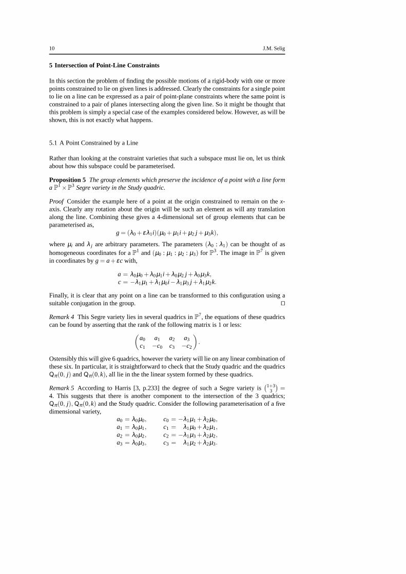
Proposition 5 The group elements which preserve the incidence of a point with a line formaP

1×P3 Segre variety in the Study quadric.

Proof Consider the example here of a point at the origin constrained to remain on thex-axis. Clearly any rotation about the origin will be such an element as will any translationalong the line. Combining these gives a 4-dimensional set ofgroup elements that can beparameterised as,

g= (λ0+ ελ1i)(µ0+µ1i +µ2 j +µ3k),

whereµi and λ j are arbitrary parameters. The parameters(λ0 : λ1) can be thought of ashomogeneous coordinates for aP1 and(µ0 : µ1 : µ2 : µ3) for P3. The image inP7 is givenin coordinates byg= a+ εc with,

a = λ0µ0+λ0µ1i +λ0µ2 j +λ0µ3k,c = −λ1µ1+λ1µ0i −λ1µ3 j +λ1µ2k.

Finally, it is clear that any point on a line can be transformed to this configuration using asuitable conjugation in the group. ⊓⊔

Remark 4This Segre variety lies in several quadrics inP7, the equations of these quadrics

can be found by asserting that the rank of the following matrix is 1 or less:(

a0 a1 a2 a3

c1 −c0 c3 −c2

)

.

Ostensibly this will give 6 quadrics, however the variety will lie on any linear combination ofthese six. In particular, it is straightforward to check that the Study quadric and the quadricsQπ(0, j) andQπ(0,k), all lie in the the linear system formed by these quadrics.

Remark 5According to Harris [3, p.233] the degree of such a Segre variety is(1+3

3

)

=4. This suggests that there is another component to the intersection of the 3 quadrics;Qπ(0, j),Qπ(0,k) and the Study quadric. Consider the following parameterisation of a fivedimensional variety,

a0 = λ0µ0, c0 = −λ1µ1+λ2µ0,a1 = λ0µ1, c1 = λ1µ0+λ2µ1,a2 = λ0µ2, c2 = −λ1µ3+λ2µ2,a3 = λ0µ3, c3 = λ1µ2+λ2µ3.

On the Geometry of Point-Plane Constraints on Rigid-Body Displacements 11

α

δ

θl

α

θ0

l

θ0

Fig. 1 Two points on two lines.

It is simple to check that this variety lies in both quadricsQπ(0, j) andQπ(0,k). How-ever, substituting the parameterisation into the Study quadric gives,

λ0λ2(µ20 +µ2

1 +µ22 +µ2

3)

Hence the intersection of all three quadrics consists of two4-dimensional varieties. For thefirst λ2 = 0 and the Segre variety discussed above is recovered. The second component ariseswhen(µ2

0 +µ21 +µ2

2 +µ23) = 0. All solutions to this condition will be complex and are thus

unphysical and can be safely ignored in the following. Whenλ0 = 0 the result is the 3-planeA∞, which lies in the Segre variety.

5.2 Two Point-Line Constraints

The intersection of two Segre varieties as found in the previous section will give a 2-dimensional variety representing the group elements whichpreserve the incidences of twopoints on a rigid body with a pair of lines. This variety can also be readily parametrised.

Proposition 6 The possible rigid-body displacements allowed by a body constrained insuch a way that two of its points are restricted to move on a pair of lines, forms a 2-dimensional variety with degree 6.

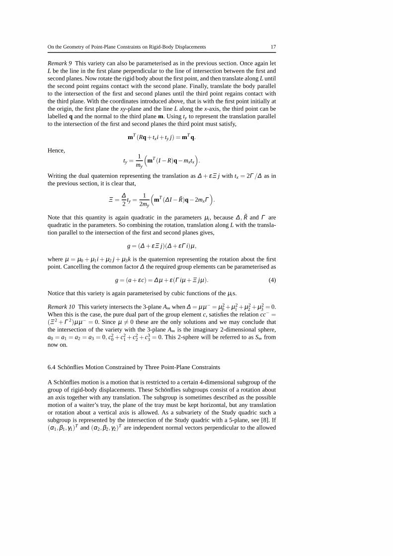
Proof The possible displacements can be split into a rotation about the axis joining thetwo points followed by a displacement of the points along their lines. To understand thedisplacement of the points along the lines it is useful to project the lines into the planeperpendicular to the common normal to the lines, see figure 1.This reduces the problem to awell known problem in planar kinematics. The motion of a rigid bar so that two of its pointremain on a pair of given lines is know as Cardan motion, see [1, ch. 9§11]. This motioncan be thought of as a rotation about the first point followed by a translation along the firstline until the second point regains contact with its line.

12 J.M. Selig

To summarise, any displacement which moves a pair of points in such a way that theyremain on a pair of given lines can be written as the product ofthree dual quaternion factors.Using the coordinates given in figure 1 the factors can be written,

g= (1+ εδ2

i)(c+sk)(c′+s′p12),

wherep12 is the unit pure quaternion corresponding to the vector joining the two points,andc′ = cos(φ/2), s′ = sin(φ/2) with φ the rotation angle about the line. The second factorgives a rotation about the vertical, the common perpendicular to the lines withc= cos(θ/2)ands= sin(θ/2). After a little trigonometry, the translation along the first axis is given by,

δ = 2l

(

cos(α −θ0)

sinα

)

sc+2l

(

sin(α −θ0)

sinα

)

s2.

Now consider the 2 dimensional variety parameterised as above as a subvariety of theSegre variety formed by the first point moving on the first line. The bidegree of this sub-variety can be found by projecting onto the two factors of theSegre variety. Projecting onto theP3 of rotations about the origin gives a two dimensional variety parameterised as(c+sk)(c′+s′p12). This is again a product, this timeP1×P

1; the standard quadric inP3.Projecting to theP1 of translations along thex-axis gives another degree 2 variety. Hencewe can conclude that the homology of this subvariety is givenby, 2α1β1+2α0β2, where asusual the homology ofP1×P

3 is generated by elementsαiβ j , where 0≤ i ≤ 1 and 0≤ j ≤ 3.As a subvariety ofP7, the intersection of the two Segre varieties is a 2-dimensional

variety with degree,

2

(

20

)

+2

(

21

)

= 2×1+2×2= 6,

see [3, p. 240]. ⊓⊔

5.3 Three Point-Line Constraints

Finding the number of positions that a rigid body can adopt sothat three of its points lie onthree particular lines is now straightforward. All that is needed is to intersect threeP1×P

3

Segre varieties. This is best done in one of the Segre varieties.

Corollary 9 In general, there are 8 ways that a rigid-body can be positioned so that 3 givenpoints of the body lie on 3 particular lines, each point lyingon its own particular line.

Proof As shown above, the intersection of two of these Segre varieties is a surface withhomology 2α1β1+2α0β2. The intersection of two of these surfaces, that is the intersectionof two Segre varieties with a third, will have homology,

(2α1β1+2α0β2)2 = 8α0β0.

That is, eight solutions can be expected in general. ⊓⊔

This result is consistent with those given by Zsombor-Murray and Gfrerrer [11] whoconsider the ‘spatial double triangular mechanism’.

On the Geometry of Point-Plane Constraints on Rigid-Body Displacements 13

6 Intersection of Point-Plane Constraints

In this section the intersection of several point-plane constraints is considered. This is theproblem considered by Wampler [10] where the degrees of these intersections are computedusing numerical techniques. Wampler uses several different models for the group of rigiddisplacements and so it is difficult, in general, to compare results.

Here the intersection with the Study quadric is considered so the homology class ofthe constraint as a subvariety of the Study quadric is often the appropriate invariant to find.The homology of the non-singular quadrics was found by Ehresmann [2]. The restriction ofthis general result to the case of the Study quadric can be found in [7, §11.5]. Essentially,the homology is generated by a single class in each dimensionexcept dimension 3. Thehomology of a 3 dimensional subvariety of the Study quadric is an integer sum of twoclassesσA andσB. The two sets of 3-plane generators of the six-dimensional quadric areknow asA-planes andB-planes, the class of anA-plane isσA and similarlyσB is the class ofa singleB-plane. The generic intersections of these generator planes leads to the intersectionformulasσA∩σB = σ0 the class of a point, andσA∩σA = σB∩σB = 0. The intersectionof the Study quadric with a hyperplane inP7 gives a five dimensional subvariety with classσ5. Similarly, the intersection with a 5-plane give a subvariety with classσ4. A tangent 4-plane intersect the Study quadric in anA-plane and aB-plane, more generally a 4-plane willintersect the Study quadric in a subvariety with classσA+σB. It is not hard to see that if a4 or 5-dimensional subvariety has classdσ4 or eσ5 then as a subvariety ofP7 the space willhave degree 2d and 2e respectively. Also a 3-dimensional subvariety with homology classdaσA+dbσB will have degreeda+db as a subvariety ofP7. In dimensions less that 3, thehomology of the Study quadric and the degree inP

7 are effectively the same, for example acurve in the Study quadric with class 2σ1 is simply a conic inP7.

6.1 One Point-Plane Constraint

The homology class of a single point-plane constraint, as a subvariety of the Study quadricis simply 2σ5. This is because the subvariety consists of the intersection of the Study quadricwith a quadric hypersurface.

Proposition 7 The set of group elements which maintain the incidence of a point with aplane lie on a variety which is the projection of the Segre varietyP2×P

3 in P11 toP

7.

Proof This set of group elements can also be easily parameterised as a product of an arbi-trary rotation about the point followed by a translation in the plane. To keeps computationssimple let us assume that the point under consideration in initially located at the origin andthe plane in question is thexy-plane. The possible group elements satisfying the constraintcan then be written as the dual quaternion,

a+ εc=(

λ0+ ε(λ1i +λ2 j))

(µ0+µ1i +µ2 j +µ3k),

whereλi andµ j are real parameters. Expanding the product gives,

a = λ0µ0+λ0µ1i +λ0µ2 j +λ0µ3kc = −(λ1µ1+λ2µ2)+(λ1µ0+λ2µ3)i+

(λ2µ0−λ1µ3) j +(λ1µ2−λ2µ1)k.

14 J.M. Selig

Notice that the coefficients of the quaternionsa andc are all separately linear in theλi andµ j parameters. It is straightforward to check that such group elements do indeed satisfy theconstraint and of course the Study quadric. Now consider theparameters(λ0 : λ1 : λ2) and(µ0 : µ1 : µ2 : µ3) as homogeneous coordinates for aP

2 and aP3 respectively. The standardSegre embedding ofP2 ×P

3 in P11 is given by assigning each of the 12 homogeneous

coordinates inP11 a termλi µ j where 0≤ i ≤ 2 and 0≤ j ≤ 3, see [3, p. 25]. Clearly theeight linear functions of theλi µ j cannot span all 12 possible combinations. There must be alinear space of 4λi µ js not appearing in the in the parameterisation. Geometrically this canbe thought of as a projection to aP7 with aP3 as centre. ⊓⊔

6.2 Two Point-Plane Constraints

Consider the set of rigid displacements which preserve the incidence of a pair of points witha pair of planes. Note that the planes will, in general, intersect in a line. Consider a line in thefirst plane perpendicular to the line of intersection. Let uscall this lineL. Now the possiblerigid displacements can be split into a displacement which preserves the incidence of the firstpoint with the lineL and the second point with the second plane, followed by a translationparallel to the intersection line of the two planes. As shownabove the set of displacementswhich constrain a point to a line form a Segre varietyP

1 ×P3. The displacements which

also constrain a second point to lie on a plane will form a 3-dimensional subvariety of theSegre variety, call this subvarietyX say. It is useful to consider the geometry ofX first.

Lemma 1 The the 3-dimensional variety X has degree 7.

Proof The varietyX is the intersection of the Segre varietyP1×P3 with a quadratic con-

straintQπ(p,n). Coordinates can be chosen so that the first point is initially located at theorigin, the first plane coincides with thexy-plane and the line of intersection between thetwo planes is parallel to they-axis. In these coordinates the lineL will lie along thex-axis,so the Segre varietyP1 ×P

3 can be parameterised as in section 5.1 above, asg = a+ εcwith,

a = λ0µ0+λ0µ1i +λ0µ2 j +λ0µ3k,c = −λ1µ1+λ1µ0i −λ1µ3 j +λ1µ2k.

Now these can be substituted into the matrix equation forQπ(p,n) as in section 3.1 above.The result will be a bi-homogeneous polynomial in the parameters,λi and µ j . However,the structure of the matrix forQπ(p,n), the zero submatrix in the bottom left-hand corner,means thatλ0 will be a common factor in all terms of the equation. Hence, this factor maybe cancelled and the result will be a polynomial which is homogeneous of degree 1 in theλi variables and homogeneous of degree 2 in theµ j variables. Hence, as a subvariety of theSegre variety,X will have homology classα0β3+2α1β2. As a subvariety ofP7, the degreeof the varietyX will therefore be,

(

30

)

+2

(

31

)

= 1+2×3= 7,

see [3,§19.1]. ⊓⊔

On the Geometry of Point-Plane Constraints on Rigid-Body Displacements 15

Remark 6The homology class ofX as a subvariety of the Study quadric can be found asfollows. Recall that the Segre varietyP1 ×P

3 has degree 4, hence as a subvariety of theStudy quadric its homology class must be 2σ4. Intersecting with the quadricQπ(p,n) withhomology class 2σ5 gives a variety with class,

2σ4∩2σ5 = 4σA+4σB.

However, notice that the Segre variety and the quadratic constraint both contain the 3-planeA∞ of ideal points in the Study quadric. This 3-plane must be a component of the inter-section, but does not correspond to any physical group elements. Deleting this componentleaves a variety with class 3σA+4σB. The degree of this variety, as a subvariety ofP

7 willbe 3+4= 7 and hence we can identify this as the subvarietyX.

Remark 7It is also possible to find a parameterisation forX. With the same coordinatesas above, imagine rotating the rigid-body about the first point at the origin. This will movethe second point off its plane in general. The incidence between the second point and planecan be regained by a suitable translation alongL. Suppose the original rotation is given bya quaternion(µ0+ µ1i + µ2 j + µ3k) with arbitrary parametersµi , the corresponding 3×3rotation matrix will be,

R=1∆

µ20 +µ2

1 −µ22 −µ2

3 2(µ1µ2−µ0µ3) 2(µ1µ3+µ0µ2)2(µ1µ2+µ0µ3) µ2

0 −µ21 +µ2

2 −µ23 2(µ2µ3−µ0µ1)

2(µ1µ3−µ0µ2) 2(µ2µ3+µ0µ1) µ20 −µ2

1 −µ22 +µ2

3

,

where∆ = µ20 +µ2

1 +µ22 +µ2

3 , see for example [7,§2.2.2]. If the second point isp and thenormal to the second plane isn then the required translationt = txi, will satisfy,

nTRp+nT t = nTp.

So that,nxtx = nT(I −R)p,

with nx thex-component of the normal vectorn. Now it is convenient to write the rotationmatrix asR= 1

∆ R, whereR is the matrix displayed above with components that are quadraticfunctions of theµis. The dual quaternion representing this translation can then be written,∆ + εΓ i, where,

Γ =1

2nxnT(∆ I − R)p.

Combining this with the arbitrary rotation about the origingives a dual quaternion withcomponents,

a = ∆ µ0+∆ µ1i +∆ µ2 j +∆ µ3k,c = −Γ µ1+Γ µ0i −Γ µ3 j +Γ µ2k.

Notice that each component of this dual quaternion is a cubicfunction of the parametersµi ,since bothΓ and∆ are quadratic functions of the parameters.

Proposition 8 The variety of group elements which preserve the incidence of two pointswith two planes has degree 8.

Proof It is easy to see that such a variety must have homology class 2σ5∩2σ5 = 4σ4 andhence as a subvariety ofP7 will have degree 8. ⊓⊔

16 J.M. Selig

Remark 8As described above, the required group elements can be splitinto an elementfrom the subvarietyX followed by an arbitrary translation in the direction of theline ofintersection between the two planes. With coordinates as above, this can be written as a dualquaternion,

g= (ν0+ εν1 j)(

(∆ µ0+∆ µ1i +∆ µ2 j +∆ µ3k)+ ε(−Γ µ1+Γ µ0i −Γ µ3 j +Γ µ2k))

,

whereν0 andν1 are arbitrary constants (not both zero). Whenν1 = 0 the varietyX is re-covered, but whenν0 = 0 the result is a point on the 3-planeA∞. That is a point of the form0+ε(µ0+µ1i+µ2 j +µ3k), ignoring common factors. From this it is easy to see that thein-tersection of two point-plane constraints is the join of corresponding points on the varietiesX andA∞.

6.3 Three Point-Plane Constraints

The homology computation for three point-plane constraints is simply,

2σ4∩2σ4∩2σ4 = 8σA+8σB.

However, the 3-planeA∞ is common to all point-plane quadrics. So this 3-plane must be acomponent of the three dimensional intersection.

Lemma 2 The multiplicity of the component A∞ in the intersection of three point-planeconstraints is one.

Proof To show this it is enough to show that the varietyA∞ is non-singular. The partialderivatives of a quadric of the formgTQπ(n, p)g = 0 can be written in vector form as,Qπ(p,n)g. That is, the partial derivative with respect toa0 is the first component of thevector, the partial derivative with respect toa1 is the second component and so forth. Hencethe singularities of the variety occur when the vectors,

Qπ(p1,n1)g, Qπ(p2,n2)g, Qπ(p3,n3)g, Q0g,

are linearly dependant. The last vector here comes from the partial derivatives of the Studyquadric. On the 3-planeA∞ the condition for singularity becomes simply,

det(

N1c∣

∣

∣N2c

∣

∣

∣N3c

∣

∣

∣c)

= 0.

Wherec= (c0, c1, c2, c3)T andNi is the top right-hand block of the matrix forQπ(pi ,ni).

The matrix in this equation is not identically zero soA∞ is in general non-singular and hencecan only have multiplicity 1 in the variety. ⊓⊔

Proposition 9 The set of group elements which preserve the incidence of three points on arigid body with three planes lie on a variety of degree 15.

Proof From above, the intersection of three point-plane constraints will have homologyclass 8σA+8σB. Deleting a single copy of the componentA∞ leaves a variety with homologyclass 7σA+8σB. So the degree of this variety as a subvariety ofP

7 is 7+8= 15. ⊓⊔

This result agrees with that given by Wampler [10].

On the Geometry of Point-Plane Constraints on Rigid-Body Displacements 17

Remark 9This variety can also be parameterised as in the previous section. Once again letL be the line in the first plane perpendicular to the line of intersection between the first andsecond planes. Now rotate the rigid body about the first point, and then translate alongL untilthe second point regains contact with the second plane. Finally, translate the body parallelto the intersection of the first and second planes until the third point regains contact withthe third plane. With the coordinates introduced above, that is with the first point initially atthe origin, the first plane thexy-plane and the lineL along thex-axis, the third point can belabelledq and the normal to the third planem. Usingty to represent the translation parallelto the intersection of the first and second planes the third point must satisfy,

mT(Rq+ txi + ty j) = mTq.

Hence,

ty =1

my

(

mT(I −R)q−mxtx)

.

Writing the dual quaternion representing the translation as ∆ + εΞ j with tx = 2Γ /∆ as inthe previous section, it is clear that,

Ξ =∆2

ty =1

2my

(

mT(∆ I − R)q−2mxΓ)

.

Note that this quantity is again quadratic in the parametersµi , because∆ , R and Γ arequadratic in the parameters. So combining the rotation, translation alongL with the transla-tion parallel to the intersection of the first and second planes gives,

g= (∆ + εΞ j)(∆ + εΓ i)µ ,

whereµ = µ0 + µ1i + µ2 j + µ3k is the quaternion representing the rotation about the firstpoint. Cancelling the common factor∆ the required group elements can be parameterised as

g= (a+ εc) = ∆ µ + ε(Γ iµ +Ξ jµ). (4)

Notice that this variety is again parameterised by cubic functions of theµis.

Remark 10This variety intersects the 3-planeA∞ when∆ = µµ− = µ20 +µ2

1 +µ22 +µ2

3 = 0.When this is the case, the pure dual part of the group elementc, satisfies the relationcc− =(Ξ 2+Γ 2)µµ− = 0. Sinceµ 6= 0 these are the only solutions and we may conclude thatthe intersection of the variety with the 3-planeA∞ is the imaginary 2-dimensional sphere,a0 = a1 = a2 = a3 = 0, c2

0+c21+c2

2+c33 = 0. This 2-sphere will be referred to asS∞ from

now on.

6.4 Schonflies Motion Constrained by Three Point-Plane Constraints

A Schonflies motion is a motion that is restricted to a certain 4-dimensional subgroup of thegroup of rigid-body displacements. These Schonflies subgroups consist of a rotation aboutan axis together with any translation. The subgroup is sometimes described as the possiblemotion of a waiter’s tray, the plane of the tray must be kept horizontal, but any translationor rotation about a vertical axis is allowed. As a subvarietyof the Study quadric such asubgroup is represented by the intersection of the Study quadric with a 5-plane, see [8]. If(α1,β1,γ1)

T and(α2,β2,γ2)T are independent normal vectors perpendicular to the allowed

18 J.M. Selig

rotation axis of the Schonflies motion, then the linear equations inP7 satisfied by the motionare,

α1a1+β1a2+ γ1a3 = 0, and α2a1+β2a2+ γ2a3 = 0.

Another way of putting this is that the possible rotations can be parameterised by the quater-nion a= µ0+µ1v wherev is a vector in the direction of the rotation axis.

Proposition 10 The intersection of the variety formed by three point-planeconstraints witha 5-plane which determines a Schonflies motion results in a Darboux motion.

Before proving this, note that Darboux motions are characterised by the fact that thetrajectory of any point in space moving under such a motion remain on a plane, actuallythey follow conic trajectories. It is well known that Darboux motions are represented bycertain twisted cubic curves in the Study quadric, [1, Ch. 9§3].

Proof Substitute the parameterisation of the constraint variety(4) from the previous sectioninto the two linear equations above. The result gives two possibilities, first∆ = µ2

0 + µ21 +

µ22 +µ2

3 = 0, this is the imaginary 2-sphere of ideal pointsS∞. The second possibility is thecurve given by,µ = µ0+ µ1v. Substituting this solution into (4) gives a curve in the Studyquadric where the 8 coordinates,ai , c j are given by cubic functions of the parametersµ0

andµ1. Such a curve is, in general, a twisted cubic curve.To show that this curve corresponds to a Darboux motion consider an arbitrary point

given by the dual quaternion,p0+ εp. As shown is section 2 above, the action of the groupof such a point is given by,

(a+ εc)(p0+ εp)(a−− εc−) = p′0+ εp′.

Substituting into this equation from (4) above gives,

∆ µ + ε(Γ iµ +Ξ jµ)(p0+ εp)∆ µ−+ ε(Γ µ−i +Ξ µ− j) =∆3p0+ ε∆2(µpµ−+2p0(Γ i +Ξ j)

)

,

were the relation∆ = µµ− has been used to simplify the result. Cancelling the commonfactor∆2 gives,

p′0+ εp′ = ∆ p0+ ε(

µpµ−+2p0(Γ i +Ξ j))

.

Finally substitutingµ = µ0 + µ1v, gives a curve inP3 in which all the coordinates arequadratic functions ofµ0 andµ1, since∆ , Γ andΞ are quadratic functions of these param-eters. ⊓⊔

This result appears in Zsombor-Murray and Gfrerrer [11]. Itwould be a little easier to showgiven a characterisation of the Darboux motion as a twisted cubic curve meetingS∞ in twopoints.

6.5 The Tripod mechanism

In this section the tripod mechanism studied by Wampler [10], is considered. Essentially themechanism consists of three points, at the vertices of an equilateral triangle, constrained tolie on three symmetrically disposed planes. The three planes all meet in a single line and areseparated by angles of 2π/3 radians.

On the Geometry of Point-Plane Constraints on Rigid-Body Displacements 19

Proposition 11 The possible displacements of a general tripod mechanism lie in a degree7 variety.

Proof The quadrics defining the three point-plane constraints canbe taken as,Qπ(n, p),GTQπ(n, p)G and(G2)TQπ(n, p)G2, whereG is the 8×8 matrix representing a rotation of2π/3 radians about the common line of the three planes. If we takep to be a point on thex-axis andn to be in they-direction then the common line can be taken as thez-axis andGas a rotation of 2π/3 radians about thez-axis. After some straightforward computations thequadric corresponding to the sum,Qπ(n, p)+GTQπ(n, p)G+(G2)TQπ(n, p)G2, is foundto bea0a3 = 0. That is, the quadric degenerates to a pair of hyperplanes,a0 = 0 anda3 = 0.The intersection of two point-plane constraints with a hyperplane will give a 3-dimensionalvariety in the Study quadric with homology class 4σA+4σB. Both hyperplanes contain the3-plane of ideal elementsA∞. Deleting this component gives a subvariety of class 3σA+4σB,in each case. The degree of such a variety inP

7 is just 3+4= 7.The hyperplanea0 = 0 consist of the rigid displacements with rotation angleπ, so this

component is not usually considered relevant since a practical machine would find it difficultto perform such a displacement. On the other hand, the hyperplanea3 = 0 contains the rigiddisplacements that have no rotation about thez-axis; the common line in the three planes.

⊓⊔

Again these results agree with the numerical computations in [10]. However, the resultsderived here are a little more detailed. For example, suppose that we attached a chain of threerevolute joints between the rigid body containing the threepoints of the tripod mechanismand the ground.

Proposition 12 The number of possible assembly configurations of this mechanism will be,in general, 20.

Proof The variety of rigid displacements allowed by the three-revolute chain is known tohave class 2σA+4σB, see [7, p.263]. Hence the number of assembly configurationsfor thiscomposite mechanism can be estimated to be,

(3σA+4σB)∩ (2σA+4σB) = 3×4+4×2= 20.

⊓⊔

6.6 Six Point-Plane Constraints

Here we look at the intersection of six point-plane constraints with the Study quadric.Each point-plane constraint is a quadrics of the form,gTQπ(p,n)g = 0, where the formof Qπ(p,n) is given in equation (3) above. Now suppose the normal vectors for the sixplanes aren1, n2, . . . , n6, only three of these can be linearly independent, so in general therewill be relations,

φ1n1+φ2n2+φ3n3+φ4n4 = 0,χ1n1+χ2n2+χ3n3+χ5n5 = 0,

ψ1n1+ψ2n2+ψ3n3+ψ6n6 = 0,

with φi , χi andψi some constants that are not all zero. If the quadrics are substituted intothese equations the resulting quadrics will have the form,

φ1Qπ(p1,n1)+φ2Qπ(p2,n2)+φ3Qπ(p3,n3)+φ4Qπ(p4,n4) =

(

Φ 00 0

)

,

20 J.M. Selig

where

Φ = φ1W1+φ2W2+φ3W3+φ4W4,

is some symmetric 4×4 matrix. With similar results for the other two equations. The quadricdefined by the 8×8 symmetric matrices represent cones (projectively equivalent to a cylin-der) inP7.

Proposition 13 In general there will be 8 group elements which satisfy six point-plane con-straints.

Proof The intersection of the six original quadrics is clearly thesame as the intersection ofthese cones with three of the original quadrics. The intersection of the three cones with theA-planec0 = c1 = c2 = c3 = 0 of rotations about the origin is, in general, 8 distinct points.Let us call thisA-planeA0 for short. For each of these points a point in the intersection ofall the quadrics can be found. To do this suppose that the coordinates inA0 are given bya = (a0, a1, a2, a2)

T . Now substitute the values found for intersection of the three conesainto the first three quadrics,

aTWi a+2aT

Nic= 0, i = 1,2,3

and the Study quadric,aTc = 0. For any of the 8 pointsa is known, so these are linearequations forc. The four equations for the 4 unknowns can be written in a matrix form as,

Mc= b,

whereM is the matrix with rows given by,

M =−2

aTN1

aTN2

aTN3

aT

and b =

aTW1aaTW2aaTW3a

0

.

Now sincea andc are homogeneous coordinates in aP7 we only need to solve these equa-

tions up to an overall multiplicative factor, the solution can be written,

a= det(M)a, and c= Adj(M)b

where Adj(M) represents the adjugate matrix ofM. In general, we obtain 8 distinct solutionscorresponding to the 8 intersection of the three cones withA0. ⊓⊔

Remark 11Notice that the intersection of the six quadrics with the Study quadric may con-tain additional solutions and even whole components of positive dimension, but these fea-tures can only be located in the ideal plane,A∞. Since these solutions will not be physicalgroup elements they are not really of any interest. Note alsothat the solution count hereagrees with the results of Wampler [10].

On the Geometry of Point-Plane Constraints on Rigid-Body Displacements 21

6.7 Five Point-Plane Constraints

We may treat the case of five point-plane constraints in a verysimilar fashion to the 6constraints considered above. In this case there are only two quadratic cones and their in-tersection withA0 is, in general, an elliptic quartic curve. This process of elimination is ofcourse geometrically a projection, moreover a linear projection with A∞ as the centre of theprojection. The pre-image of the projection can be recovered as above by setting,

a= det(M)a, and c= Adj(M)b.

Note that this will give a point onA∞, the centre of the projection, exactly when det(M) = 0.

Lemma 3 The determinantdet(M) = 0 if and only if aT a= 0.

Proof Notice that,

Ma=

000

aT a

,

since theNi matrices are anti-symmetric. Moreover it is easy to see thata multiple of thevectora is the only non-zero vector which is annulled by the first three columns ofM. HencewhenaT a= 0 the matrix has a non-trivial kernel. ⊓⊔

Proposition 14 The possible motions of a rigid-body subject to five point-plane constraintslie on an elliptic curve of degree 12.

Proof The equation det(M) = 0 defines a complex quadric surfaceaT a = 0, in A0. Thissurface will in general meet the elliptic quartic curve found above in 4×2= 8 points. Hencethere are in general 8 points where the curve inP

7 meets the centre of the projection. Whenthis curve is projected toA0 its degree is reduced by one for each intersection with the centreof projection. Hence, we can infer that the degree of the curve which projects to the ellipticquartic inA0 must have degree 4+8= 12. Moreover, since it is known that the genus of acurve is invariant under projections we may also conclude that this curve is elliptic. ⊓⊔

Again this result for the degree of this variety agree with the results of Wampler [10].

6.8 Four Constraints

The result in this section differs from that found by Wampler[10], although the commentmade above on the difficulty of making direct comparisons of results should be borne inmind. The result given here is however, consistent with those found in the previous sectionand in section 5.2 above.

Proposition 15 The set of group elements which preserve the incidence of four points withfour planes lie on a surface of degree 6.

Proof For 4 point-plane constraints there is just one quadratic cone in the linear system ofquadrics. The intersection of this cone with the 3-planeA0 is, in general, a non-singular 2-dimensional quadric. The intersection of this quadric withthe imaginary quadric det(M) =aT a= 0 will be an elliptic quartic curve in general. Now suppose weintersect these varieties

22 J.M. Selig

with a hyperplane inP7. In A0 the intersection with the quadratic cone will be a conic curveand the intersection with the quartic curve will be 4 points.Using the same argument as inthe previous section we may conclude that the intersection of the 4 point-plane constraintswith the hypersurface is a curve with degree 2+4= 6. So a general hyperplane section ofthis surface is a degree 6 curve, thus the degree of the surface is also 6. ⊓⊔

Remark 12The surface is birationally equivalent toP1×P1. The intersection of the cone

from the linear system of point-plane constraints withA0 gives a 2-dimensional quadric.This surface is well known to be isomorphic to the Segre variety P

1 ×P1, so this variety

can be parametrised by linear functions of the productsλi µ j wherei and j are 0 or 1. Thatis, the coordinates ofa are linear functions of theλi µ j . As above the surface inP7 can bereconstructed as,

a= det(M)a, and c= Adj(M)b.

This gives a rational map fromP1 ×P1 to the surface which inverts the projection toA0.

Notice here that the elements of the matrixM are linear functions of theλi µ j while thecoordinates of the vectorb are quadratic functions ofλi µ j .

7 Conclusions

This work has looked at general results for the intersections of point-plane constraints onrigid body displacements. There are however many special cases where these results willfail. For example, the Darboux motion mentioned in section 6.4 above is characterised bythe fact that under this motion all point of space move on non-parallel planes. Hence theremust be choices of 6 point-plane constraints whose intersection is a curve rather than eightpoints. This also applies to the infinitesimal kinematics studied in section 4. For a Darbouxmotion the zero torsion cubic must degenerate to all of space. The study of the possibledegeneracies, both for finite and infinitesimal kinematics,and the conditions under whichthey occur is important future work.

Another area of future work which follows from the above is the investigation of inter-sections of the point-sphere constraints. This has particular relevance to the kinematics ofa parallel robot manipulator known as the Gough-Stewart platform. This machine is knownto have, in general, 40 possible solutions for the position of the platform given particularlengths for the legs. That is the intersection of 6 point-sphere constraints should yield 40solutions, see [9], [4] and [5], for example.

Finally, it is hoped that the case has been made for the simpletechniques from AlgebraicGeometry that have been used here. Although more sophisticated techniques will be able totake us further these simple methods still have much to offer.

References

1. Bottema, O. and Roth, B., Theoretical Kinematics, Dover Publications, New York, (1990).2. Ehresmann, C., Sur la topologie de certaines espaces homogenes, Ann. of Math., 396–443, (1934).3. Harris, J., Algebraic Geometry a first course, Springer Verlag, New York, (1992).4. Husty, M. L., An algorithm for solving the direct kinematics of general Stewart-Gough platforms. Mech-

anism and Machine Theory,31(4):365–380, (1996).5. Mourrain, B., Enumeration problems in Geometry, Robotics and Vision, In Algorithms in Algebraic Ge-

ometry and Applications, Prog. in Math.,143:285–306, eds. L. Gonzalez and T. Recio. Birkhauser, Basel,(1996).

On the Geometry of Point-Plane Constraints on Rigid-Body Displacements 23

6. Schonflies, A., Geometrie der Bewegung in synlhetischerDarstellung. B. G. Teubner, Leipzig, (1886).{see also the review of this book by F. Morley in Bull. Amer. Math. Soc.5(10):476–480 (1899).}

7. Selig, J.M., Geometric Fundamentals of Robotics, Springer Verlag, New York, (2005).8. Selig, J.M., Quadratic Constraints on Rigid-Body Displacements, ASME Jounal of Mechanisms and

Robotics,2:041009 (7 pages), (2010).9. Wampler, C.W., Forward displacement analysis of generalsix-in-parallel sps (Stewart) platform manipu-

lators using soma coordinates. Mech. Mach. Theory31(3): 331–337, (1996).10. Wampler, C.W., On a rigid body subject to point-plane constraints, ASME J. of Mechanical Design,

128(1):151–158, (2006).11. Zsombor-Murray, P.J. and Gfrerrer, A., A unified approach to direct kinematics of some reduced motion

parallel manipulators. ASME Journal of Mechanisms and Robotics,2(2):021006 (10 pages), (2010).