On the geometry of diffusion operators andstochastic flows

K. D. Elworthy Y. Le Jan X.-M. Li

Contents

1 Construction of connections 71.1 Construction of connections . . . . . . . . . . . . . . . . . . . . . . . . 71.2 Basic Classes of Examples . . . . . . . . . . . . . . . . . . . . . . . . . 141.3 Adjoint connections, torsion skew symmetry, basic formulae . . . . . . 181.4 Example: Homogeneous spaces continued . . . . . . . . . . . . . . . . . 25

2 The infinitesimal generators and associated operators 292.1 The irrelevance of drift in dimension greater than 1 . . . . . . . . . . . 292.2 Torsion Skew Symmetry . . . . . . . . . . . . . . . . . . . . . . . . . . 342.3 The ‘divergence operator’ δ . . . . . . . . . . . . . . . . . . . . . . . . 362.4 Hormander form generators on differential forms . . . . . . . . . . . . . 402.5 On the infinitesimal generator . . . . . . . . . . . . . . . . . . . . . . . 46

2.5.1 Example . . . . . . . . . . . . . . . . . . . . . . . . . . . . . . . 462.5.2 Symmetricity of the generator Aq . . . . . . . . . . . . . . . . . 47

3 Decomposition of noise and filtering 553.1 A canonical decomposition of the noise driving a stochastic differential

equation . . . . . . . . . . . . . . . . . . . . . . . . . . . . . . . . . . . 553.2 Canonical decomposition of the Gaussian field Wt . . . . . . . . . . . . 583.3 Filtering out redundant noise . . . . . . . . . . . . . . . . . . . . . . . 61

3.3.1 When A does not belong to the image of X . . . . . . . . . . . 673.3.2 The inverse derivative flow . . . . . . . . . . . . . . . . . . . . . 693.3.3 Integrability of certain Cr norms for compact M . . . . . . . . . 693.3.4 The semigroup on forms: Bochner type vanishing theorems . . . 713.3.5 Bismut formulae . . . . . . . . . . . . . . . . . . . . . . . . . . 72

4 Application: Analysis on spaces of paths 744.1 Integration by parts and Clark-Ocone formulae . . . . . . . . . . . . . 764.2 Logarithmic Sobolev Inequality . . . . . . . . . . . . . . . . . . . . . . 804.3 Analysis on Cid(DiffM) . . . . . . . . . . . . . . . . . . . . . . . . . . . 81

5 Stability of stochastic dynamical systems 85

6 Appendices 92A Universal Connections as L-W connection . . . . . . . . . . . . . . . . 92B Creation and Annihilation operators (notation for section 2.4) . . . . . 97

1

C Basic formulae . . . . . . . . . . . . . . . . . . . . . . . . . . . . . . . . 99D List of notation . . . . . . . . . . . . . . . . . . . . . . . . . . . . . . . 106

2

Introduction

The concepts of second order semi-elliptic operator, Markov semi-group, diffusion pro-cess, diffusion measures on path spaces essentially give different pictures of the samefundamental objects, with related Riemannian or sub-Riemannian geometry. Here weconsider a different layer of structure centred around the concepts of sums of squaresof vector fields, stochastic differential equations, stochastic flows and Gaussian vectorfields; again essentially equivalent, and this time with associated metric linear connec-tions on tangent bundles and subbundles of tangent bundles. The difference betweenthese two levels of structure can be seen from the fact that if a semi-elliptic differentialoperator on functions on a manifold M is given a representation as a sum of squareof vector fields (“Hormander form”) it automatically gets an extension to an operatoron differential forms. In exactly the same way representing a diffusion process as theone point motion of a stochastic flow determines a semi-group acting on differentialforms (by pulling the form back by the flow and taking expectation.) Given a regu-larity condition there is an associated linear connection and adjoint ‘semi-connection’in terms of which these operators can be simply described (e.g. by a Weitzenbockformula) as can many other important quantities (e.g. existence of moment expo-nents for stochastic flows). Moreover in the stochastic picture the connections remainrelevant in the collapse from this level to the simpler one giving new results and newproofs of results e.g. on path space measures.

In more detail: Chapter 1 is connected with the construction of linear connectionsof vector bundles as push forwards of connections on trivial bundles. This is a directanalogue of the classical and elementary construction of the covariant derivative of avector field on a submanifold of Euclidean space, leading to the Levi-Civita connec-tions (Example 1B). Narasimhan & Ramadan’s theorem of universal connections isevoked to assure us that all metric connections can be obtained this way (Theorem1.1.2). We then go on to consider the various forms in which this construction willappear in situations described above. (E.g. how certain Gaussian fields of sectionsdetermine a connection.) Homogeneous spaces give a good class of examples describedin some detail in §1.1 B. The notion of adjoint connection or semi-connection on asubbundle E of the tangent bundle TM to our underlying manifold M is described in§1.3. A semi-connection allows us to differentiate vector fields on M in E-directions.They play an important role in the theory. One difficulty is that the adjoint of ametric connection may not be metric for any metric (Corollary 1.3.7). In generalHormander type hypoellipticity conditions on our generator A, or equivalently on E,play little role in this article. However in Theorem 1.3.9 we show how they are related

3

to the behaviour of parallel translations with respect to associated semi-connections.

In chapter 2 we concentrate on a generator A given in Hormander form, and itsassociated stochastic differential equation (s.d.e.). A first result is Theorem 2.1.1which shows in particular that (for dimM > 1) any elliptic diffusion operator can bewritten as a sum of squares with no first order term, or equivalently that any ellipticdiffusion is given by a Stratonovich equation with no drift term. The extension Aq

of A to q-forms is shown to have the form Aq = −(dδ + δd) for a certain operator δfrom q-forms to q − 1 forms (Proposition 2.3.1) and also a Weitzenbock form Aq =12trace∇2 − 1

2Rq (if there is no drift term A) (Theorem 2.4.2). Driver’s notion of

torsion skew symmetry is investigated in §2.2 in order to discuss the operators δ, andwhen they are L2 adjoints of the exterior derivative d, in §2.3. Later, §3.3.3, thesemigroups associated to these operators are used to obtain Bochner type vanishingtheorems under positivity conditions on Rq.

The question of the symmetricity of Aq with respect to some measure on M isdiscussed in §2.5.2. Theorem 2.5.1 gives a fairly definitive result for Aq with the zeroorder terms removed. However conditions under which Rq is symmetric seem not soeasy to find if q > 1. For q = 1 this reduces to symmetricity of the Ricci curvatureRic which is shown in Proposition C.6 of the Appendix to hold in the torsion skewsymmetric case if and only if the torsion tensor T determines a coclosed differential3-form, c.f. [Dri92]. These sections are not used later in this article.

The main applications in stochastic analysis start with Chapter 3. The basic ideais that the diffusion coefficient of an s.d.e often has a kernel: so that there is “redun-dant noise” from the point of view of the one point motion. We extend the resultsfrom the gradient case in [EY93] to our more general, possibly degenerate, situationgiving a canonical decomposition of the noise into its redundant and non-redundantparts. We then show how this can be used to filter out the redundant noise in gen-eral situations. (This filtering out corresponds to the collapse in levels of structurementioned above.) On the way we have to discuss conditional expectations of vectorfields along the sample paths of our process, Definition 3.3.2. All this is done in somegenerality, e.g. allowing for the possibility of explosion. The main application is to thederivative process Tξt of a stochastic flow: Theorem 3.3.7 and Theorem 3.3.8. Whenthe redundant noise is filtered out the process becomes a “damped’ or Dohrn-Guerratype parallel translation using the associated semi-connection. This procedure worksequally for the derivative of the Ito map ω 7→ ξt(x0)(ω) in the sense of MalliavinCalculus from which follow integration by parts theorems for possibly degenerate dif-fusion measures, Theorem 4.1.1. For gradient systems, using [EY93], this method wasused by [EL96] and was suggested by [AE95]. The Levi-Civita connection appears inthat case (which is why gradient systems behave so nicely), but in the degenerate casewhich is allowed here the connections are on arbitrary subbundles of TM and there isno unique particularly well behaved connection to use. Hypoellipticity is not assumed.The “admissible” vector fields are those which satisfy a natural “horizontality” con-dition, §4.1 B and §4.1 C. Closely related is a Clark-Ocone formula (Theorem 4.1.2)expressing suitably smooth functions on path space as stochastic integrals with respect

4

to the predictable projection of their gradient. From this we use the method given in[CHL] to obtain a Logarithmic Sobolev inequality for our diffusion measures, Theorem4.2.1. Our “damping” of the parallel translation means that no curvature constantsappear: indeed since in general we have no Riemannian metric given on M it wouldbe unnatural to have such constants. Logarithmic Sobolev inequalities automaticallyimply spectral gap inequalities and the constancy of functionals with vanishing gra-dient (or equivalently whose derivatives vanish on admissible vector fields), Corollary4.1.3: a non-trivial result even for Frechet smooth functions on path space for thecase of degenerate diffusions. In Theorem 4.1.1 the corresponding results are provedfor the measures on paths on the diffeomorphism group DiffM of M coming fromstochastic flows, or equivalently from Wiener processes on DiffM [Bax84].

Chapter 5 is concerned with applications to stability properties of stochastic flows.In particular upper and lower bounds for moment exponents are obtained in termsof the Weitzenbock curvatures of the associated connection and a generalization ofthe second fundamental form to our situations: Theorem 5.0.5. This gives a criterionfor moment stability in terms of ‘stochastic positivity’ of a certain expression in thequantities with consequent topological implications: Corollary 5.0.6.

A weakness of these results is that we usually require the adjoint semi-connectionto be metric for some metric. Theorem 5.0.7 shows that the lack of this conditionreally is reflected in the behaviour of the flow.

Chapter 6 consists of technical appendices. The first gives a detailed descriptionof how the push forward construction of connections we use relates to Narasimhan& Ramanan’s pull back of the universal connections. This is needed in the proof ofTheorem 1.1.2. The other appendices give the notation of annihilation and creationoperators used in the discussion of the Weitzenbock curvatures in section 2.4 and somebasic formulae and curvature calculations for connections given in the L-W form.

The connection determined by a non-degenerate stochastic flow first appeared in[LJW84]: for this reason we have called it the LeJan-Watanabe or L-W connection. Itwas also discovered in the context of quantum flows in [AA96] and for sums of squaresof vector fields in [PVB96]. It is used for analysis on loop spaces in [Aid96]. For thenon-degenerate case many of the results given here were described in [ELJL97a] withannouncements for degenerate situations in [ELJL97b]. They were stimulated by[EY93]. The Chentsov-Amari α-connections in statistics are rather different. Theyare in general non-metric if α 6= 0 and torsion free, see [Ama85], pp42, 46.

Acknowledgement: The authors would like to thank MSRI, Institut HenriPoincare and Universitaet Bochum (as well as their home institutes) for hospitalityduring the completion of this project. Support is acknowledged from EU grant ERBFMRX CT 960075 A, NSF grant DMS-9626142, Alexander Humboldt-Stiftung, andthe British Council.

K. D. ELWORTHY, MATHEMATICS INSTITUTE, UNIVERSITY OF WARWICK, COVENTRY

CV4 7AL, UK

5

Y. LE JAN, DEPARTMENT DE MATHEMATIQUE, UNIVERSITE PARIS SUD, 91405 ORSAY,

FRANCE

XUE-MEI LI, DEPARTMENT OF MATHEMATICS, UNIVERSITY OF CONNECTICUT, 196

AUDITORIUM ROAD, STORRS, CT 06269 USA. e-mail address: xmli@math.uconn.edu

6

Chapter 1

Construction of connections

We consider connections on a C∞ vector bundle E over a smooth manifold M deter-

mined by a split surjection of vector bundles HY←−−→ E −→ 0 where H = M × H is

the trivial bundle with fibre a Hilbertable space H. The characterization of such aconnection ∇ is that for each x ∈M

∇v (X(·)e) ≡ 0 all v ∈ TxM and e ∈ ImageY (x) .

When M and E are finite dimensional and E has a Riemannian metric all metricconnection on E can be obtained this way for some finite dimensional H. Theseconnections can also be considered to be induced by Gaussian measures on the spaceof C∞ sections of E. In §1.2 and §1.4 some basic examples are given. They describethe connections arising from certain Gaussian fields, operators in Hormander form,stochastic differential equations, and homogeneous space structures.

For E a subbundle of TM there is also an adjoint ’semi-connection’ ∇, investigatedin §1.3. In particular we show ∇ is metric with respect to some Riemannian metricon M if and only if for one set of x0, y0 ∈ M and T > 0 the parallel translation //t

using ∇ along ξT,y0t (x0), the solution ξt(x0) to the stochastic differential equation

dxt = X(xt) dBt conditioned to satisfy ξT (x0) = y0, is a bounded L(Tx0M,Ty0M)-valued process.

1.1 Construction of connections

A. Consider a C∞ manifold M , a C∞ vector bundle π : E → M over M and a C∞

vector bundle homorphism X : H → E of a trivial bundle H = M × H, where His a Hilbertable space. We will consider only real bundles (and manifolds) here. Atthis stage M,E,H could be infinite dimensional (but separable, with M metrizable);however our main focus will be on cases with M and E finite dimensional. In thissituation we shall write n = dim M , p = fibre dimension of E, with m = dim H ifdim H <∞.

Suppose X is surjective and Y a chosen right inverse to X

7

HY←−−→ E −→ 0.

Our situation is very similar to a special case of that of Harvey and Lawson in[HL93]. Let Γ(E) denote the space of smooth sections of E, and set Ex = π−1(x), x ∈M . Write X(x) = X(x, ·) : H → Ex. For u in E let Zu be the section given by

Zu(x) = X(x)Y (π(u))u. (1.1.1)

Proposition 1.1.1 There is a unique linear connection ∇ on E such that for allu0 ∈ Ex0 , x0 ∈ M the covariant derivative of Zu0 vanishes at x0. It is the ’pushforward’ connection defined by

∇v0Z = X(x0)d (Y (·)Z(·)) (v0), v0 ∈ Tx0M, Z ∈ Γ(E) (1.1.2)

where d refers to the usual derivative d (Y (·)Z(·)) : TM → H of the map Y (·)Z(·) :M → H.

Proof. Certainly (1.1.2) defines a covariant differentiation. Let ∇ be any linearconnection on E. We have

Z(·) = X(·)Y (·)Z(·)

whence, for v ∈ Tx0M ,

∇vZ = X(x0)d (Y (·)Z(·)) (v) + ∇v [X(·) (Y (x0)Z(x0) )]

= ∇vZ + ∇vZZ(x0).

(1.1.3)

Since ∇ is assumed to be a genuine connection (not just a covariant differentiation:a point only relevant if E is infinite dimensional) and since also the map

TM × E → E

(v, u) 7→ ∇vZu

gives a smooth section of the bundle of bilinear maps L(TM,E;E) we see that ∇ isa smooth connection on E, (e.g. [Eli67]). Taking ∇ = ∇ in (1.1.3) we see that ∇ hasthe property required. Uniqueness also follows from (1.1.3). //

B. We shall be mainly interested in metric connections. These will arise in two,essentially equivalent, forms which we will call the metric form and the Gaussian formrespectively. However the examples coming from homogeneous spaces are more easilyunderstood in the more general non-metric framework and these will also be describedbelow, in §1.2.

In the “metric” form H is now a Hilbert space, inner product 〈, 〉 ≡ 〈, 〉H and sothe surjective homomorphism X induces a Riemannian metric 〈, 〉x : x ∈M on E.The right inverse Y is chosen to be the adjoint of X, Y = X∗.

8

Theorem 1.1.2 Let H be a Hilbert space, and Y the adjoint of X with respect tothe induced metric on E by X. Then the connection ∇ is adapted to the Riemannianmetric. Moreover if M and E are finite dimensional any metric connection for anyRiemannian metric on E can be obtained this way from some such X with H somefinite dimensional Hilbert space.

Proof. Take a vector field U and a vector v ∈ Tx0M . Then

d 〈U, U〉 (v) = 2〈d (Y (·)U(·)) (v), Y (x0)U(x0)〉

= 2〈X(x0)(d (Y (·)U(·)) (v), U(x0)〉 = 2〈∇vU, U〉.

This shows that ∇ is metric. The fact that any metric connection arises this wayin the finite dimensional situation comes from Narasimhan and Ramanan’s theorem[NR61] on universal connections. In the finite dimensional case the connection ∇ isprecisely the pull back of the universal connection over the Grassmanian G(m, p) ofp-planes in H by the map x 7→ [ image of Y (x) : Ex → H]; for details see §A inthe Appendix. Narasimhan and Ramanan show that any metric connection can beobtained as such a pull back.

In this situation we shall call ∇ the LeJan-Watanabe or L-W, connection deter-mined by X, or by (X, 〈, 〉), for reasons described at the end of §1.3B below.

Example 1B (Gradient systems). Let j : M → Rm be an immersion. Define

X(x) : Rm → TxM to be the orthogonal projection of R

m on TxM , identified withits image under the differential dj of j, so that X(x)e = grad〈X(·), e〉Rm using theinduced metric on M . Then Y (x) : TxM → R

m is the inclusion, Tj, and we havethe classical construction of the Levi-Civita connection for this metric.(That it hasno torsion can also be seen from the formula (2.2.3) below.)

C. For the ‘Gaussian form’ suppose we have a mean zero Gaussian field W ofsections of E. In its most general form W would be a section of the pull back p∗E ofΓ(E) over the projection p : Ω×M →M where (Ω,F , P ) is a probability space. ThusWx(ω) := W (ω, x) ∈ Ex for each x ∈ M , ω ∈ Ω. We will assume that W (ω, ·) is C∞

for each ω ∈ Ω. The more concrete manifestation comes from a Gaussian measureγ on some subspace of the C∞ sections of E. Then (Ω,F , P ) = (Γ(E),F , γ), thecanonical space, for F the σ-algebra of cylindrical subsets of Γ(E), and we identifyWx with the evaluation map ρx : Γ(E) → Ex, given by ρx(U) = U(x). See [Bax76].For any suitable function f on Γ(E) we write Ef or Ef(W ) for

∫Ωf(W (ω, ·))P (dω)

(equivalently∫Γ(E)

f(U)dγ(U) in the canonical picture). Let γx be the law of Wx, a

Gaussian measure on Ex. We make the nondegeneracy assumption that each γx isnon-degenerate and so in the finite dimensional case has the form

γx(B) = (2π)−p/2

∫

B

e−〈y,y〉2xdy

for some 〈, 〉x on Ex.

9

Proposition 1.1.3 There is a unique connection ∇γ on E such that the randomvariable ∇γ

vW is independent of W (x0) for any v ∈ Tx0M , x0 ∈ M . It is given interms of the conditional expectation by

∇γvZ =

d

dtE W (x0) |W (σ(t)) = Z(σ(t)) |t=0; (1.1.4)

or equivalently

∇γvZ =

d

dtEW (x0) 〈W (σ(t)), Z(σ(t))〉σ(t)

∣∣∣∣t=0

(1.1.5)

for any C1 curve σ with σ(0) = v, v ∈ Tx0M , and is adapted to the metric 〈, 〉x, x ∈M.Moreover(i) Let Hγ be the reproducing kernel Hilbert space of γ, then ∇γ is the L-W connectionfor (X, 〈, 〉Hγ

) where X(x, h) = ρx(h) = h(x).(ii) If E is a finite dimensional vector bundle over a finite dimensionalM every metricconnection can be considered as ∇γ , given by (1.1.4), for some Gaussian measure γon Γ(E) with finite dimensional support.

Proof. Recall that the reproducing kernel Hilbert space Hγ of γ is the same as theCameron-Martin space H of γ and is a Hilbert space, here necessarily consisting ofC∞ functions. Among its standard properties are:

(i) The restriction of ρx to H maps onto Ex, each x ∈ M and induces the innerproduct 〈, 〉x. It will also be denoted by ρx.

(ii) The reproducing kernel k, a section of the vector bundle

∪x∈M,y∈ML(Ex, Ey) →M ×M,

defined by the reproducing property that k(x, ·)(v) belongs to H each v ∈ Ex and forall h ∈ H,

〈k(x, ·)v, h〉Hγ= 〈h(x), v〉x, (1.1.6)

is also the covariance of γ:

k(x, y)v = E〈W (x), v〉xW (y), v ∈ Ex, x, y ∈M. (1.1.7)

See [Bax76]. From (1.1.7) we see

k(x, y)W (x) = E W (y)|W (x) ∈ TyM (1.1.8)

and so

k(x, ·)v = E W (·) |W (x) = v ∈ H ⊂ Γ(E) (1.1.9)

for all v ∈ Ex, and x, y ∈M .

10

From this we see that the defining equation (1.1.4) or (1.1.5) for ∇γvZ can be

written

∇γvZ =

d

dtk(σ(t), x0)Z(σ(t)) |t=0 (1.1.10)

=d

dtEW (x0) 〈W (σ(t)), Z(σ(t))〉σ(t)

∣∣∣∣t=0

. (1.1.11)

If we set X(x) = ρx so X : H → E we see from (1.1.6) that the adjoint map Y toX, using the induced Riemannian metric is just k:

Y (x) = ρ∗x = k(x, ·) : Ex → H

k(x, y)(·) = X(y)Y (x) : Ex → Ey.

We are therefore in the ’metric’ form discussed in Theorem 1.1.2 and ∇ is just theL-W connection ∇ of ρ, 〈, 〉Hγ

.

For the characterization in terms of the independence of ∇ZW and W observethat for u ∈ Ex0 the reproducing vector field Zx0,u, or Zu as in (1.1.1) in the metricform, is given by

Zu(y) = X(y)Y (x0)u = k(x0, y)u (1.1.12)

= E W (y) |W (x0) = u (1.1.13)

so that for any linear connection ∇ on E we have

∇vZu = E

∇vW |W (x0) = u

.

Thus if v ∈ Tx0M we have ∇vZu = 0 for all u if and only if

E〈∇vW,W (x0)〉x0 = 0

since ∇vW and W (x0) are Ex0-valued Gaussian random variables (this is exactly thecondition for the independence of W (x0) and ∇vW ). By Proposition 1.1.1 this provesuniqueness, i.e. that ∇vW and W (x0) are independent for all x0 and v ∈ Tx0Mimplies ∇ = ∇γ . It also shows that

E〈∇γvW,W (x0)〉x0 = 0, for all v ∈ Tx0M , all x0 ∈M, (1.1.14)

which, again because they are Gaussian vectors, implies that ∇γvW is independent of

W (x0) for all v ∈ Tx0M , x0 ∈ M . (The fact that the processes W (x0) and ∇γvW (x0)

both take values in fibres Ex0 of a bundle causes no difficulty in using the standardresults we used: to reduce to the standard situation where the process takes values in afixed Hilbert space H0, say, either observe that we can find a measurable trivializationθ : E → M × H0 some H0, 〈〉0 with each θx : Ex → W0 an isometry or simply notethat we have given to us:

Y : E →M ×H

11

which isometrically maps each Ex onto a subspace of H: so we can take H0 = H. Inthis second way we can simply treat Γ(E) as a subspace of the space of maps of Minto H.)

Finally, to show that all such metric connections arise this way, let〈, 〉x : x ∈ M be a smooth metric on E, with a metric connection ∇. By Theorem1.1.2 there is a Euclidean space R

m, 〈〉 and anX : M×Rm → E whose L-W connection

is ∇. Let γm be the standard Gaussian measure of Rm, 〈, 〉, and let γ be the image

measure on Γ(E) of γ under the map Rm → Γ(E), e 7→ X(·)e. We claim ∇γ = ∇.

Indeed if k is the reproducing kernel for γ then if u ∈ Ex

k(x, y)u =

∫

Rm

〈X(x)e, u〉xX(y)(e) dγm(e)

= X(y)Y (x)u

for Y (x) = X(x)∗. Thus by (1.1.12) the definitions of the vector fields Zu defined viaX and via γ agree and so ∇γ = ∇ by their defining property.

Remark 1C. The proof above shows the essential equivalence between the “met-ric” and “Gaussian” forms. It also shows that the connection depends only on thelaw, γ, of the process (or equivalently on the subspace H of Γ(E) together with itsinner product) not on the process itself. The case of H a Hilbert space of sections ismore intrinsic than that of a mapping of a Hilbert space into the space of sections,and often the Gaussian formulation is simpler to use, especially when H is infinite di-mensional. However it is often the “metric” form which arises in practice, for examplein the gradient systems of example 1B.

Example 1C: Gaussian vector fields on Rn are said to be isotropic if they are

invariant in law under Euclidean transformations. The covariance of an isotropicGaussian vector field on R

n is determined by two spectral measures FL and FN onR

+. It is given by the formula

E(W i(x)W j(y)

)= Cij(x− y) (1.1.15)

with

Cij(z) =

∫

R+

∫

Sn−1

e iρ〈z,u〉 [uiujσ(du)FL(dρ) + (δij − uiuj)σ(du)FN(dρ)] ,

σ being the uniform distribution on Sn−1. The vector field W (x, ω) has an almost sureC∞ version when the measures FL and FN have moments of all orders. From formula(10) in [ELJL97a] or remarks in §1.3 B below (or rather from its generalization to theGaussian field case) we see that

Γij,k(x0) = 0.

The connection so constructed is therefore trivial. The isotropic stochastic flows,associated with W was studied in [Jan85] and [BH86]. A special case had first beenintroduced in [Har81], using an approximation by discrete vortices.

12

However, even in that isotropic case, nontrivial connections arise if you considerthe motion of several points:

In general, the Gaussian field W can be extended into a Gaussian field W (d) onM (d) = (x1, x2, . . . , xd) ∈ Md|xi 6= xj, for i 6= j as follows. There is a canoni-cal isomorphism between T(x1,x2,...xd)M

(d) and the direct sum ⊕dα=1Txα

M . With thisidentification, we can set W (d)(x1, x2, . . . , xd) = ⊕d

α=1W (xα).For the isotropic fields on R

n,

W (d)(x1, x2, . . . , xd) = ⊕dα=1

n∑

i=1

W i(xα)∂

∂xαi

.

It is always a nondegenerate Gaussian vector except in dimension one, when thespectral measure is atomic. See e.g. Darling [Dar92]. We can define an associatedmetric on (Rn)(d)

〈u, v〉(x1,...,xd) = 〈K−1u, v〉,

where 〈, 〉 denotes the Euclidean metric and K−1 is the inverse of the matrix of co-variances:

K(α,i),(β,j) = Cij(xα − xβ), 1 ≤ α, β ≤ n, 1 ≤ i, j ≤ d.

The L-W connection ∇(d) is a metric connection on (Rn)(d) for the metric constructedabove. The computations below show it is not the Levi-Civita connection. Fromthe result of §3.3 we can see it is related to a solution to a filtering problem: Giventhe paths of d points, the restriction to the path of one of the points of the dampedadjoint parallel transport along the path of the d-point motion is the restriction ofthe derivative flow of d-point motion conditioned on the d-point motion.

The connection can be computed explicitly. For example when d = 1, by (1.1.4),the Christoffel symbols of ∇(d) are

Γγα,β =

∂

∂t|t=0 EW (xγ) |W (xλ + tδλα) = δλβ for all λ.

For α 6= γ, Γγα,β clearly vanishes. Moreover

Γαα,β =

∂

∂t|t=0

([K(t, α)]−1

)β,λC(xα − xλ + t δα

λ )

with ([K(t, α)])λ,λ′ = C (xλ − xλ′ + tδαλ − tδα

λ′). Hence, setting K(0)λλ′ = C(xλ − xλ′)

and K ′(0, α) =∂

∂tK(t, α)|t=0

Γαα,β =

(K(0)−1K ′(0, α)

)β,α

.

For d = 2 one checks that in particular,

Γ112 =

−C ′(x1 − x2)

1 − C2(x1 − x2)

and

Γ111 =

−C(x1 − x2) · C′(x1 − x2)

1 − C2(x1 − x2).

13

1.2 Basic Classes of Examples

Example A: Sums of squares of vector fields: operators in Hormanderform. For a particular manifestation of our basic class of examples consider a secondorder differential semi-elliptic operator A on M given in the Hormander form

A =1

2

m∑

1

LXjLXj + LA. (1.2.1)

where X1, . . . , Xm, A are smooth vector fields on M , with LV denoting Lie differenti-ation in the direction of a vector field V . We obtain

X : Rm → TM

by

X(x)e =∑

j

〈e, ej〉Xj(x)

for e1, . . . , em the standard orthonormal base for Rm. If we assume Ex := X(x)[Rm]

has constant rank we are in the metric form situation, obtaining a connection ∇ onthe resulting subbundle E = Image X of TM .

The geometry of such operators have been examined from a different viewpoint (seee.g. [Str86]), usually with a hypoellipticity assumption. They are usually consideredas operators on functions. However the presentation of A in the form (1.2.1) showshow to extend it to more general tensors, in particular to differential forms on M . Weshow below in section 2.4 the relevance of ∇ to the analysis of these operators.

Example B: Connections arising in the theory of stochastic flows. LetD be the space of C∞ diffeomorphisms of M with C∞ topology making it a Polishtopological space, (see [Bax84]). Following Baxendale [Bax84] consider a Brownianmotion, ξt : t ≥ 0, on D, i.e. a stochastic process on D satisfying

1. almost sure continuity in t,

2. independent increments on the left, i.e. ξtξ−1s and ξvξ

−1u are independent if

0 ≤ s < t ≤ u < v,

3. time homogeneity;

4. ξ0=identity.

For each x ∈ M there is the process ξt(x) : t ≥ 0 on M which was shownto be a diffusion with generator A, say. Similarly on M × M there is a process(ξt(x), ξt(y)) : t ≥ 0 for each (x, y) ∈ M × M giving a diffusion with generator

14

A2 say. It turns out that for f, g : M → R both C∞ with compact support then onf ⊗ g : M ×M → R, defined by (x, y) 7→ f(x)g(y),

A2 (f ⊗ g) (x, y) = A(f)(x)g(y) + f(x)A(g)(y) +1

2Γξ ((df)x, (dg)y)

where Γξ : T ∗M × T ∗M → R is the symmetric bilinear map given by

Γξ ((df)x, (dg)y) = limh↓0

E(f(ξh(x)) − f(x)) (g(ξh(y)) − g(y))

h. (1.2.2)

If we assume that A is elliptic, its symbol, which is quadratic and given byΓξ ((df)x, (df)x), will be non-degenerate and so determines a metric on TM . Raisingand lowering indices of Γξusing this metric gives a section k of the bundle L(TM ;TM)over M ×M ,

〈k(x, y)v1, v2〉y = Γξ (〈v1,−〉x, 〈v2,−〉y) , v1 ∈ TxM, v2 ∈ TyM. (1.2.3)

Following LeJan and Watanabe [LJW84] we can define a connection ∇ξ on TMby

∇ξvZ =

d

dtk(σ(t), x0)Z(σ(t)) |t=0 (1.2.4)

just as in equation (1.1.10). Indeed it was shown in [Bax81] (without assuming ellip-ticity) that Γξ is the covariance for a Gaussian measure γ on Γ(TM), mean γ, andthat there is a correspondence between Brownian motions on D and such Gaussianmeasures, at least for M compact, see also [Kun90]. Given sufficient regularity thecorrespondence is obtained via the stochastic differential equation

dxt = ρxt dWt + γ(xt)dt

where Wt : t ≥ 0 is the Wiener process on Γ(TM) associated to γ, and ρx theevaluation map at x ∈ M , or equivalently for the stochastic differential equation onD for the flow ξt : t ≥ 0

dξt = (TRξt) dWt + TRξt

(γ)dt

where Rh refers to right translation (i.e. composition) by the diffeomorphism h. Itwas shown in [LJW84] that the generator A is given by

A(f)(x) =1

2tr∇ξ(df)(x) + df(γ(x)).

In particular ξ is determined by Γξ and γ. Given our non-degeneracy assumptions wesee ∇ξ = ∇γ, (of course ellipticity can be replaced by constancy of the rank of thesymbol).

Remark:Recall that γ vanishes if and only if ξt is equal in law to ξ−1

t for any fixed t.

15

Example C: Stochastic differential equations (s.d.e.). The form in whichwe will most frequently be using the theory will come from stochastic differentialequations

dxt = X(xt) dBt + A(xt)dt (1.2.5)

where Bt is a Rm-valued Brownian motion, A is a smooth vector field and indicatesthe integral involved being Stratonovich. For x0 in M let ξt(x0) : 0 ≤ t < ρ(x0) bea maximal solution from x0, so that ρ(x0) ∈ (0,∞] is the explosion time from x0.There is the associated semigroup Pt : t ≥ 0: for bounded measurable functionsPtf(x) = Ef(ξt(x))χt<ρ(x) with generator A = 1

2

∑m1 LXiLXi + LA, e.g. Example A

above. If M is compact the solutions can be chosen (they are only defined up to setsof measure zero) to give a solution flow of diffeomorphisms as described above: thoughby taking B· to be a finite dimensional Brownian motion we lose some generality.

The equation (1.2.5) will be said to be regular (or non-singular) if X has constantrank.

Example B: Homogeneous spaces. Suppose we have an action of a Lie groupK on M . Let k be the Lie algebra of K (taken to be the tangent space at the identity)and exp : k → K the exponential map. We have the induced map

X : M × k → TM

given by

X(x)(e) =d

dt(exp te · x) |t=0

so that e 7→ Xe := X(·)e is a Lie algebra homomorphism. For g ∈ K let Lg denoteleft multiplication by g acting on K or on M and let Rg be right multiplication by gacting on K. There is the adjoint action

ad ≡ adK : K → GL(k)

given byad(g)e = (TRg)

−1 TLg(e), e ∈ k, g ∈ K.

Note that if x ∈M , g ∈ K and e ∈ k then

X(gx)e =d

dtexp te · gx |t=0 = TLg

d

dtg−1 (exp te) g · x |t=0 (1.2.6)

= TLgd

dtexp t ad (g−1)(e) · x |t=0 (1.2.7)

= TLgX(x)(ad(g−1)e

). (1.2.8)

Suppose further that the action is transitive, and also fixing x0 ∈M the mappingK →M , g 7→ g · x0 identifies M with K/H for H = g ∈ K : g · x0 = x0 making Ma homogeneous space which is also reductive i.e. there is a linear splitting

k = h + m, (1.2.9)

16

with h∩m = 0, where h is the Lie algebra of H and m some linear subspace of k whichis adH invariant:

ad(g) [m] = m, all g ∈ H.

Note that h = ker X(x0), so by (1.2.8), for g ∈ K,

ker X(gx0) = ad (g)[h]. (1.2.10)

The reductive property allows us to define mx := ad (g) [m] ⊂ k for x = gx0 since ifx = ghx0, so h ∈ H, we have

ad(gh) [m] = ad (g)ad (h) [m] = ad (g)[m].

Thus we have the splittingk = KerX(x) + mx

for each x ∈ M and we can define Y (x) : TxM → k to be the inverse of the restrictionof X(x) to mx.

Proposition 1.2.1 The connection ∇ induced on TM by X, Y is K invariant. If k

admits an adK-invariant inner product 〈, 〉 for which m is orthogonal to h then ∇ isthe L-W connection for X, 〈, 〉.

Remark: This applies to spheres and Grassmanian manifolds in which cases theconnections are the Levi-Civita connections. See Theorem 1.4.8 below.

Proof. First observe from (1.2.8) that

ad (g)Y (x)TLg−1 : TgxM → k

has image in mgx and is a right inverse to X(gx). Thus

Y (gx) = ad (g)Y (x)TLg−1 . (1.2.11)

From this and (1.2.8), for g ∈ K, Z a vector field on M , and v ∈ TxM we have

∇g∗(v)g∗(Z) = X(gx)d(Y (·)TLgZ

(g−1·

))TLg(v)

= TLgX(x) ad (g−1)d(Y (·)TLgZ

(g−1·

))TLg(v)

= TLgX(x)d(Y (g−1·)Z

(g−1·

))TLg(v)

= TLgX(x)d (Y (·)Z(·)) (v)

= g∗

(∇vZ

).

Thus ∇ is K-invariant.When 〈, 〉 is adK-invariant, if m is orthogonal to h then mx ⊥ ker X(x) for each

x and we see Y (x) = X(x)∗, from which it follows that ∇ is the L-W connection forX, 〈〉.

These connections on homogeneous spaces are discussed further in §1.4 below.

17

1.3 Adjoint connections, torsion skew symmetry,

basic formulae

A. From now on in this section we shall assume that E is a subbundle of the tangentbundle TM of M . Then for any linear connection ∇ on E there is an operation whichgives a differentiation of arbitrary smooth vector fields V in E-directions: define

∇′uV = ∇V (x0)U + [U, V ](x0), u ∈ Ex0 (1.3.1)

where U is any section of E with U(x0) = u. In terms of the Lie derivative LV ,mappings sections U of E into vector fields,

∇′V = ∇V − LV , (1.3.2)

c.f. the tensor AV defined on p.235 of [KN69a]. It is easy to see that ∇′V ∈ΓHom(E, TM), or see [KN69a], p.235, and also that ∇′U is a derivation on Γ(M)over C∞(M) for each U ∈ Γ(E). We shall call such an operation a semi-connectionon E and call ∇′ the adjoint (semi)connection to ∇. Adjoint connections were intro-duced in the case E = TM by Driver in [Dri92].

When E = TM it is a genuine connection: indeed, by definition, in this case forvector fields U, V we have

[U, V ] = ∇′UV − ∇V U (1.3.3)

whence

∇′uV = ∇uV − T (u, V (x0)). (1.3.4)

Here T : TM × TM → TM is the torsion tensor of ∇, defined by

−T (u, v) = [U, V ](x0) − ∇uV + ∇vU, (1.3.5)

where v = V (x0), c.f. Proposition 2.3 of [KN69a].

When E is a genuine subbundle there is still a skew symmetric

T : E ⊕ E → TM

defined by (1.3.5) with U, V now sections of E, (and so, also vector fields on M). Forour semi-connection ∇′ we can again define T ′ : E ⊕ E → TM by equation (1.3.5).It is immediate from (1.3.3) and (1.3.5) that T ′ = −T .

Coming back to the specific case of a connection ∇ as in §1.1 note for any v, u ∈ E,∇vZ

u = ∇uZv ≡ 0. So

T (u, v) = −[Zu, Zv]. (1.3.6)

The canonical example of adjoint connections are given on Lie groups G: theadjoint of the flat right invariant connection on TG is the flat left invariant connection(and conversely). More examples are given in §1.3E below.

The name ’semi-connection’ is justified by:

18

Proposition 1.3.1 Let E⊥ be a complementary subbundle to E in TM , so TM =E ⊕ E⊥. Let ∇⊥ be any linear connection on E⊥ and let ∇1 be the direct sumconnection induced on TM : ∇1 = ∇ ⊕ ∇⊥. Let ∇1′ be the adjoint connection to ∇1.Then

∇′uV = (∇1)′uV, u ∈ Ex0 , V ∈ Γ(TM).

Proof. This follows from equation (1.3.1) since if U ∈ Γ(E) and V ∈ Γ(TM) then∇V U = ∇1

V U .

From this proposition we see immediately that it is possible to define operationsD′

∂ton smooth vector fields vt : t ∈ [0, T ] along piecewise C1 curves σ in M with

σ(t) ∈ Eσ(t) for each t (“horizontal” curves) such that: if V ∈ Γ(TM) and vt = V (σ(t))then

D′vt

∂t= ∇′σ(t)V.

For example simply take ∇⊥ as in the proposition to obtain (∇1)′ with correspond-ing D1′

∂tand then restrict to horizontal curves observing the result is independent of the

choice of E⊥ and ∇⊥. Alternatively there are partially defined “Christoffel symbols”,see Remarks in the next subsection. Similarly there are parallel translations

//′t : Tσ(0)M → Tσ(t)M,

which are linear isomorphisms, but only defined along horizontal curves and indeed,as usual,

D′vt

∂t= //′t

d

dt//′−1

t vt.

A vector field vt : t ∈ [0, T ] along such a curve is parallel if and only if D′vt

∂t=

0. Proposition 1.3.1 will enable us to be confident in applying the usual rules ofconnections to ∇′ in consequence. The following extension of (1.3.3) will be of basicimportance.

Lemma 1.3.2 For S > 0, T > 0, let σ : [0, S] × [0, T ] → M be C1 with σ(s, ·)horizontal for each s ∈ [0, S]. Then

D′

∂t

∂σ

∂s=D

∂s

∂σ

∂t. (1.3.7)

Proof. By Proposition 1.3.1, we can assume E = TM . Then

D

∂t

∂σ

∂s=D

∂s

∂σ

∂t+ T (

∂σ

∂t,∂σ

∂s).

19

But, from (1.3.4),D′

∂t

∂σ

∂s=D

∂t

∂σ

∂s− T (

∂σ

∂t,∂σ

∂s).

In general //′

t does not map fibres of E to fibres of E:

Proposition 1.3.3 For the adjoint semi-connection ∇′ the following are equivalent:

1. ∇′uV ∈ E whenever V ∈ Γ(E) and u ∈ E.

2. //′

t maps Eσ(0) → Eσ(t) whenever σ is a horizontal path.

3. T maps E ⊕ E to E.

4. E is an integrable foliation and ∇ restricts to a connection on each of its leaves.

If so ∇′ restricts to a connection on the leaves of E.

Proof. Certainly (4) implies (1). Also (1) implies (3) by (1.3.4) and if (3) holdsthen [U,Z] ∈ Γ(E) when E,Z ∈ Γ(E) by (1.3.5) and (1) holds by (1.3.4), so (3)implies (4). To take in (2) observe that (2) implies (3) using (1.3.4) and the formulaD′vt

∂t= //

′

tddt//′t−1vt, while (4) immediately implies (2).

Remark: If P : TM → TM/E is the projection of TM onto the quotient bundlethen by (1.3.5)

P(T (u1, u2)

)= −P

([U1, U2](x)

)(1.3.8)

for U1, U2 ∈ Γ(E) with U1(x) = u1, U2(x) = u2. Thus P T is independent of theconnection on E. It is a well known invariant of the subbundle, e.g. see Strichartz[Str86].

B. Suppose now we have HY←−−→ E −→ 0 as in §1.1A, but still with E a subbundle

of TM . The adjoint ∇′ of the associated connection ∇ will be denoted by ∇, withparallel translation // etc. It takes on a particularly simple form using the sectionsZu : u ∈ E of E defined in (1.1.1):

Lemma 1.3.4 1. For any vector field V and u ∈ Ex0 we have

∇uV = LZuV,

2. Let σ : [0, T ] →M be a horizontal curve with σ(0) = x0. Then //tv0 = Tx0Sσt (v0)

all v0 ∈ Tx0M , where Sσt : M →M, 0 ≤ t ≤ T is the flow of the time dependent

vector field Z σ(t) = X(·)Y (σ(t))σ(t).

20

Proof. Part (1) is immediate from (1.3.1) or (1.3.2), the defining property of ∇, (that∇Zu vanishes at x0), and the skew symmetry of Lie differentiation of vector fields

LZuV = [Zu, V ] = −LV Zu.

For part (2) set xt = Sσt (x0) and vt = Tx0S

σt (v0). Since

ddtSσ

t (x0) = X(Sσt (x0))Y (σ(t))σ(t)

Sσ0 (x0) = x0

we see xt = σ(t). Also by Lemma 1.3.2

Ddtvt = ∇vt

X (Y (σ(t))σ(t)) = 0vt|t=0 = v0

.

by the defining property of ∇. Thus vt : 0 ≤ t ≤ T is parallel for ∇.

Remarks:(1). Since Lie differentiation with respect to a fixed vector field obeys the usual

derivation rules a corollary of Lemma 1.3.4 (1) is that, when E = TM , for any smoothtensor field A on M

∇uA = LZuA. (1.3.9)

For the general case, for u ∈ E we could define ∇uA, for example, by using Proposition1.3.1 and then (1.3.9) will still hold; or more directly we could use (1.3.9) as thedefinition.

(2). By expanding U over the basis, Lemma 1.3.4 (1) reads

∇UV = [Zu, V ] =

m∑

1

[X i, V ]〈X i, U〉, U ∈ Γ(E), V ∈ Γ(TM); (1.3.10)

or in the Gaussian form,∇UV = E[W,V ]〈W,U〉. (1.3.11)

By (1.3.3),∇V U = [V, U ] + E[W,V ]〈W,U〉. (1.3.12)

(3). For X : Rm → E ⊂ TM as described let ∇ be the Levi-Civita connection for

some Riemannian metric on M (or indeed any torsion free connection on TM). Thenfor U ∈ Γ(E), V ∈ Γ(TM), V (x0) = v, U(x0) = u,

∇vU = X(x0)d (Y (·)U(·)) (v)

= ∇vU +X(x0)∇vY (U(x0))

= ∇vU + Γ(v, u),

21

say. Also by definition, (1.3.1),

∇uV = ∇vU + [U, V ](x0)

= ∇vU + Γ(v, u) + ∇uV − ∇vU

= ∇uV + Γ(v, u).

Working in a chart (U, φ) of M with Xφ the local representation of X

Xφ = Tφ X : φ(U) × Rm → Tφ[E] ⊂ φ(U) × R

n

etc. and taking ∇ to be the usual differentiation in Rn this shows that ∇ has “Christof-

fel symbols” given by

Γφx0

(v, u) = Xφ(x0)DYφ(x0)(v)(u) (1.3.13)

where now v ∈ Rm and u ∈ Tx0φ(Ex0), x0 ∈ U . Moreover

∇uV = DV φ (φ(x0)) u+ Γφx0

(Tx0φ(v), Tx0φ(u)) (1.3.14)

Equivalently in the nondegenerate case

Γijk = −

m∑

r=1

n∑

l=1

∂X(x0)r,i

∂xjX(x0)

r,`gk`, (1.3.15)

where X(x)r,i, 1 ≤ i ≤ n, 1 ≤ r ≤ m is the matrix representing X(x) : Rm →

R, i.e. X(x)r,i = 〈X(er), fi〉 for ei and fi orthonormal bases for Rm and TxM

respectively, and gk` the metric tensor. This shows that ∇ is the L-W connectiondefined in [LJW84].

C. It will be important to know when ∇ is adapted to some Riemannian metric〈, 〉′ on TM , (see also §2.1) in the sense that

d 〈Z1(·), Z2(·)〉′ (u) =

⟨∇uZ1(x), Z2(x)

⟩′x

+⟨Z1(x), ∇uZ2(x)

⟩′x

(1.3.16)

for u ∈ Ex and all Z1, Z2 ∈ Γ(TM), or equivalently that parallel translation //t alongany smooth horizontal curve preserves 〈, 〉′. In the case that E = TM and 〈, 〉′ = 〈, 〉,when this holds ∇ is said to be torsion skew symmetric. See §2.2. Let ∇′ be theLevi-Civita connection for 〈, 〉′.

Proposition 1.3.5 The adjoint ∇ is adapted to 〈, 〉′ if and only if ∇′Zu is skewsymmetric on TxM, 〈, 〉′x for all u ∈ Ex, x ∈M .

Proof. By Lemma 1.3.4 (2), ∇ is adapted to 〈, 〉′ if and only if

d

dt

⟨TSσ

t (v10), TS

σt (v2

0)⟩′

σ(t)

∣∣∣t=0

= 0

for all horizontal curves σ and v10, v

20 in Tσ(0)M . But this is precisely the condition

⟨∇′v1

0Z σ(0), v2

0

⟩′σ(0)

+⟨v10 , ∇

′v20Z σ(0)

⟩′σ(0)

= 0,

since D′

∂tTSσ

t (v10) = ∇′Z σ(0) if D′ is differentiation with respect to ∇′.

22

Corollary 1.3.6 Suppose X(x) is injective for each x ∈ M . Then ∇ is adapted tosome Riemannian metric 〈, 〉′ on TM if and only if Xe ≡ X(·)(e) is an infinitesimalisometry for each e ∈ H.

Proof. Injectivity implies that Xe = Zu for u = X(x0)e, any x0 ∈ M . Butskew-symmetry of ∇′Xe is equivalent to Xe being an infinitesimal isometry (e.g. see[KN69a], p.237).

Remark 2C. Note that in the Gaussian form, §1.1C, the injectivity hypothesisbecomes the assumption that the vector fields in the reproducing kernel Hilbert spaceHγ of γ never vanish. In this case ∇ is the trivial connection determined by the

trivialization Y of E and so the curvature R of ∇ vanishes (alternatively ∇W vanishesand R is seen to vanish by the expression given in Appendix I of [ELJL97a], see alsoProposition C.4 in Appendix C). In the stochastic flow picture, §1.2F, it implies thatfor any x0 ∈ M , and T > 0 the infinite dimensional process ξt : 0 ≤ t ≤ T can beexpressed in terms of ξt(x0) : 0 ≤ t ≤ T. The standard probabilistic approach tosecond order elliptic operators on R

n is to use such X taken to be the positive squareroot of the symbol of the operator considered as a map of R

n into the positive definitesymmetric matrices.

Corollary 1.3.7 SupposeX is injective but the Lie algebra generated by X e : e ∈ Hhas dimension greater than 1

2n(n+ 1) when n = dimM <∞. Then ∇ is not adapted

to any Riemannian metric on M .

Proof. The Lie algebra of infinitesimal isometries of a connected Riemannianmanifold has dimension at most 1

2n(n+ 1) ([KN69a],Theorem 3.3 on p238).

Example 2C. For M = R2 define vector fields X1, X2 by X1(x, y) = ∂

∂x,

X2(x, y) = x3 ∂∂x

+ ∂∂y

. This gives an injective X as in §1E and the Lie algebra gen-

erated by X1, X2 is easily seen to be infinite dimensional. Thus the induced adjointconnection ∇ is not adapted to any metric. This example could easily be modifiedoutside of a compact set to make it periodic, and so project to a compact surface.

D. Consider the stochastic differential equation

dxt = X(xt) dBt + A(xt)dt, (1.3.17)

where Bt is a Rm-valued Brownian motion, A is a smooth vector field and indicatesthe integral involved being Stratonovich. Let ξt(x0) be the solution with initial valuex0 and ∇ the connection constructed from X. Then roughly speaking the paralleltranslation along the paths of ξt is bounded if and only if ∇ is adapted to someRiemannian metric. (This statement is true for smooth paths as easily seen from theproof of the next theorem). See also Theorem 5.0.7 for the corresponding result onthe derivative flow.

23

Theorem 1.3.8 Assume that X is nondegenerate and the stochastic differential equa-tion (1.3.17) does not explode. For x0, y0 ∈M and T > 0, let ξT,y0

t (x0) : 0 ≤ t ≤ T

be the process conditioned to be y0 at time T of ξt(x0) and let //t =: //t

T,x0,y0

be par-

allel translation along ξT,y0t (x0). If ∇ is adapted to some Riemannian metric then

//T is a bounded L(Tx0M,Ty0M) valued random variable for such x0, y0 and T > 0.

Conversely if just for one set of x0, y0 and T > 0 the parallel translation process //T

along the path of ξT,y0t (x0) is bounded then ∇ is adapted to some Riemannian metric

on M .

Proof. The ‘if’ part is clear since //T would be an isometry.

Suppose that //T is bounded. Let u0 be a frame at x0 and P (u0) the holonomybundle through u0, i.e.

P (u0) = u ∈ GL(M) | there exists a horizontal curve from u0 to u.,

with structure group

Φ(u0) = g ∈ GL(n) | u0 · g ∈ P (u0).

We can reduce ∇, now a genuine connection, to a connection on P (u0). Let (ut) bethe solution to

dut = X(ut) dBt + A(ut)dt

with initial value u0. Here X and A are the horizontal lifts in P (u0) of X and A.Then ut : 0 ≤ t ≤ T is the horizontal lift of ξt(x0) : 0 ≤ t ≤ T.

The support of the law µt(P ) of uT is all of P (u0) by the Stroock-Varadhansupport theorem and the definition of P (u0). Consequently by Carverhill [Car88] thesupport of uT when ξT (x0) is conditioned to have ξT (x0) = y0 is π−1

0 (y0), whereπ0 : P (u0) → M is the projection. Thus parallel translations from Tx0M to Ty0Malong the paths of the conditioned process ξy0

T (x0) : 0 ≤ t ≤ T are dense in thespace of parallel translations along smooth paths. So the latter is a bounded setand Φ(u0) is bounded in GL(n). As a consequence there is an inner product onR

n, 〈, 〉′ say, invariant under Φ(u0). The required metric at a point z of M is then〈v1, v2〉z = 〈u−1v1, u−1v2〉′ for any u ∈ π−1

0 (z).

E. Proposition 1.3.3 was concerned with the case when E is integrable. At theother extreme is the situation where the vector fields X1, . . . , Xm together with theiriterated brackets span TxM for each x in M , giving hypoellipticity of the operatorA by Hormander’s theorem. Bismut showed how this hypoellipticity was reflectedin the behaviour of the derivative of the associated stochastic flow so that Lemma1.3.4 (2) makes it not surprising that it is also reflected in the behaviour of parallel

translation //s along the paths of the associated diffusion, as we see next. As beforewe consider the stochastic differential equation (1.3.17) and assume it to be regularwith A(x) ∈ Ex for each x in M . Our discussion is an adaptation of that in [Bel87]which was in turn based on [Bis81].

24

Let Rt(ω) = span//−1

s X(xs)e : e ∈ Rm, 0 ≤ s ≤ t∧ τ ∈ Tx0M where τ is a fixed,

positive predictable stopping time less than the explosion time for our stochasticdifferential equation. By Proposition 1.3.3 in the integrable case Rt(ω) = Ex0 foreach t ≥ 0. In general let Ex0 ⊂ Tx0M be the linear span of X1(x0), . . . , X

m(x0)together with all the brackets and iterated brackets of the vector fields X 1, . . . , Xm

evaluated at x0 (this depends only on E → TM , not on ∇ or a choice of X1, . . . , Xm

determining E):

Theorem 1.3.9 For each t > 0,

Ex0 ⊂ Rt(ω) almost all ω in Ω.

Proof. Set R(ω) = ∩t>0Rt(ω). By the Blumenthal 0-1 law there exists a non-random R0 ⊂ Tx0M with R0 = R(ω) almost surely. Moreover there therefore existsa predictable stopping time τ1 with 0 < τ1 < τ such that Rt(ω) = R0 for 0 ≤ t ≤ τ1almost surely.

Suppose ` ∈ T ∗x0M annihilates R0. Then for e ∈ R

m, with Xe := X(·)e,

`(//−1

s Xe(xs)) = 0, 0 ≤ s ≤ τ1.

Now if Z is a vector field with `(//−1

s Z(xs)) = 0, 0 ≤ s ≤ τ1, taking the localmartingale part of its canonical decomposition we have

`(//−1

s ∇X(xs)fZ) = 0

all f ∈ Rm, 0 ≤ s ≤ τ1.

By Lemma 1.3.4 (1) this gives

`(//−1

s [Z,Xf ](xs)) = 0, 0 ≤ s ≤ τ1, (1.3.18)

since [Z,Xf ] = [Z,ZXf

] + ∇ZXf and //

−1

s ∇ZXf ∈ R0 because ∇ZX

f ∈ Exs. Taking

Z = Xe show that [Xe, Xf ](x0) ∈ R0 each e, f ∈ Rm. Repeating the argument, using

(1.3.18) with Z = [Xe, Xf ] gives [ [Xe, Xf ], Xg ](x0) ∈ R0 for all e, f, g in Rm, and the

full result follows by induction.

1.4 Example: Homogeneous spaces continued

A. For an important class of examples we will go back to situation of a reductive ho-mogeneous space M = K/H described in §1.2 using the notation there. In Proposition1.2.1 we saw from our construction that the action of K determines a K-invariant con-nection on M and that given an adK-invariant inner product on k the L-W connectionis K-invariant: in particular the metric 〈 〉X (i.e. induced by X(x) : k → TM ) isK-invariant, as is seen from (1.2.8). In general given an inner product 〈 〉 on k themetric 〈 〉X induced on TM will not be K-invariant.

25

Proposition 1.4.1 A K-invariant connection ∇ on M is uniquely determined by themapping

m → L(Tx0M ;Tx0M)

given by

e 7→ ∇′Xe∣∣∣Tx0M

,

where ∇′ is the adjoint connection.

Proof. Observe that for any vector field Z on M

AZ : TM → TM

defined by AZ(v) := −∇vZ − T (Z, v) as defined in [[KN69a], p255, [KN69b], p188]is given by AZ(v) = ∇′vZ. The result is then a reformulation of Corollary 2.2 of[[KN69b], p191].

B. The K-invariant connection on M corresponding to the identically zero map:m → L(Tx0M ;Tx0M) is the canonical connection

Theorem 1.4.2 Let ∇ be the connection on M determined as in §1.2 by its reduc-tive homogeneous space structure and let ∇ be its adjoint. Then ∇ is the canonicalconnection. In particular

(i). R(u, v)w = −[[Zu, Zv] − Z [Zu,Zv], Zw

], u, v, w ∈ Tx0M ,

(ii). ∇T = 0,(iii). ∇R = 0.

Proof. Take ∇ = ∇ in Proposition 1.4.1 and use the defining property of ∇ to see ∇is the canonical connection. For (i), (ii) and (iii) see Theorem 2.6 p193 [KN69b] anduse the fact that e 7→ Xe(·) is a homomorphism of Lie algebras.

Corollary 1.4.3 Any K-invariant tensor on M is ∇-parallel.

Proof. See Proposition 2.7 p192 of [KN69b].

From this we immediately have

Corollary 1.4.4 The connection ∇ is metric for any K-invariant metric on M .

Taking ∇ = ∇ we can obtain in this way a class of metric connections whoseadjoints are not metric for any metric on M .

C. Suppose next that as well as being reductive there is an adH-invariant innerproduct B on m. We then obtain a K-invariant Riemannian metric on M whichagrees with B under the isomorphism m → Tx0M . The space, together with B, iscalled naturally reductive if it has a decomposition as before with also

B(α, [β, γ]

m

)+ B

([β, α]

m, γ)

= 0, α, β, γ ∈ m (1.4.1)

where the subscript m refers to the projection in k onto m.

26

Proposition 1.4.5 The decomposition k = m + h together with B is naturally reduc-

tive if and only if ∇ is torsion skew symmetric for the induced K-invariant metric onM .

Proof. ⟨T (u, v), w

⟩x0

= −〈[Zu, Zv] (x0), w〉x0, u, v, w,∈ Tx0M

by (1.3.6). Set α = Y (x0)u, β = Y (x0)v, γ = Y (x0)w. Then

[Zu, Zv] (x0) =[Xα, Xβ

](x0)

= X(x0) ([α, β])

= X(x0)([α, β]

m

)

and the result follows from (1.4.1).

Corollary 1.4.6 In the naturally reductive case ∇ is a torsion skew symmetric con-nection.

Note however that the metric involved may not be induced, via X, by an innerproduct on k. However from [KN69b] p203 Theorem 3.5 we see that if k has an adK-invariant inner product 〈 〉, we can let m = kerX(x0)

⊥ = h⊥ to have K/H naturallyreductive with B(α, β) = 〈α, β〉, α, β ∈ m. Thus

Theorem 1.4.7 Let k have an adK-invariant inner product 〈 〉. Then the L-W con-nection on M determined by X, 〈〉 is torsion skew symmetric and K-invariant. Itsadjoint connection is the canonical connection of the corresponding reductive homoge-neous space structure.

D. Specializing further suppose that we have a symmetric space (K,H, σ): soK,H are as before with a reductive decomposition k = m + h such that m and h are,respectively, the −1 and +1 eigenspaces for the involution σ of k.

Theorem 1.4.8 For a symmetric space ∇ and ∇ are torsion free. In particular theyare the Levi-Civita connection of any K-invariant Riemannian metric on M .

Proof. That T = −T = 0 follows from (1.3.6) and the fact that [m,m] ⊂h,see Proposition 2.1 p226 [KN69b], or from the corresponding fact for the canonicalconnection [KN69b] p231 Theorem 3.2. The result follows from Corollary 1.4.4.

Corollary 1.4.9 Let the symmetric space (K,H, σ) be such that k has an adK-invariantinner product 〈 〉 invariant under σ. Then the L-W connection for X, 〈〉 is the Levi-Civita connection for the induced metric (which is K-invariant).

27

Proof. In this situation m ⊥ k, see [[KN69b], p233], and so mx ⊥ KerX(x) foreach x ∈ M : thus Y = X∗ and ∇ is the L-W connection and hence metric. Since itis torsion free it is Levi-Civita.

Example 1.4.1 Lie groups as symmetric spaces

Recall the standard symmetric space structure for a Lie group G. Let∆G = (g, g) ∈ G×G : g ∈ G. Let G×G act on G by

(g, h) · x = gxh−1.

The stabilizer of e is ∆G and G has the homogeneous space structure G = G×G/∆G,and symmetric space structure with involution induced from σ : G × G → G × Ggiven by σ(g, h) = (h, g). For example the symmetry se : G→ G is just x 7→ x−1, see[KN69b] (p228).

The relevant decomposition of k = g ⊕ g is

k = ∆g ⊕ m

where ∆g = (α, α) : α ∈ g, m = (α,−α) : α ∈ g, see [KN69b] (p198). Now sup-pose g and hence g × g has an adG-invariant inner product 〈 〉.

The stochastic differential equation on G is

dxt = TLxt dBt − TRxt

dB′t

for (B·), (B′·) independent BM(g). The flow is given by ξt(x) = gtxg′−1t for

dgt = TRgt dBt

dg′t = TRgt dB′t

with g0 = e = g′0.The flow consists of isometries so that the moment exponents are zero. However

for G with bi-invariant metric (as we are considering), if g has trivial centre thenRic > 0. Thus we obtain a class of stochastic differential equations such that(i) Ric > 0;(ii) all moment exponents vanish;(iii) ξ· consists of isometries;(iv) ∇ is the Levi-Civita connection.In particular (i) and (ii) can be contrasted with results which says that negativecurvature implies first moment exponent positive. They also give an example wherethe hypotheses of Corollary 6.4.7 in [Li92] hold.

Remark: Among other homogeneous spaces with a Riemannian space struc-ture are the spheres Sn = SO(n + 1)/SO(n), oriented Grassmannian manifoldsSO(p+ q)/SO(p) × SO(q) and hyperbolic spaces O(1, n)/SO(n).

28

Chapter 2

The infinitesimal generators andassociated operators

For any second order elliptic operator L with smooth coefficients and L1 ≡ 0 on amanifold M of dimension greater than 1, we construct X : R

m → TM , for somem, such that L = 1

2

∑m1 LXjLXj , the differential generator for the solutions of the

stochastic differential equation without drift dxt = X(xt) dBt. This result is, infact, proved for a class of semi-elliptic operators. In section 2.4 the Holmander formoperator Aq = 1

2

∑j LXjLXj + LA on differential q-forms is analysed. Section §2.2

discusses a special class of connections on TM and also the natural generalization δof δ to our situation. We show in §2.4 that Aq = −1

2(dδ + δd) + LA so that when the

L-W connection associated to X is the Levi-Civita connection and A = 0 then Aq isthe De Rham-Hodge Laplacian. In the regular case there is the Weitzenbock formula:

Aqφ =1

2trE∇·(∇·φ) + LAφ−

1

2Rqφ

for Rq a zero order term, the ’Weitzenbock curvature’ related to ∇. In the lastsection we give conditions for the leading order terms of Aq to be symmetrizable asan operator on a suitable L2 space. In particular we show that this holds if A0 issymmetrizable and ∇ is metric for some metric on TM .

2.1 The irrelevance of drift in dimension greater

than 1

A. The first application of the construction in section §1.1 is that any elliptic dif-ferential operator can be considered as an infinitesimal generator to some stochasticdifferential equation with zero drift: dxt = X(xt) dBt. Let E be a subbundle of TMwith fibre dimension p. Let Z be a E-valued vector field, and V : R

m → E ⊂ TM aC∞ surjection. Consider the operator L on M :

L =1

2

m∑

1

LV iLV i + LZ , (2.1.1)

29

where V i = V (ei) for an orthonormal base of Rm.

Theorem 2.1.1 Assume p > 1. For L as given above, there is a map X : M×Rm →

TM linear in the second variable such that the solution to dxt = X(xt) dBt has Las infinitesimal generator, i.e. L = 1

2

∑j LXjLXj .

Given E the Riemannian metric induced by V . Recall that a diffusion ξt(x) :0 ≤ t < ρ(x) generator L is a ∇ martingale if f(ξt(x)) − traceE∇df(ξt(x)) is a localmartingale for any smooth f : M → R. (e.g. [Eme89]). An immediate corollary of theTheorem is that a diffusion ξt(x) : 0 ≤ t < ρ(x), x ∈ M, whose generator satisfiesthe conditions of Theorem 2.1.1 is a ∇-martingale for some metric connection ∇ on E.In fact (as will be seen explicitly in §3.3), ξt(x0) will be the stochastic development ofa Brownian motion on Ex0 using ∇. The existence of a connection on TM for whichthis is true for a non-degenerate diffusion was shown by Ikeda-Watanabe [IW89] and amodification of their construction for the case E = TM is one of the main ingredientsof our proof. The other key ingredient is Narasimhan & Ramanan’s theorem onuniversal connections used via Theorem 1.1.2.

The proof is given in §§C below. To adapt Ikeda & Watanabe’s construction weneed the modification of the classical result on connections given in Proposition 2.1.2below. Its proof taken up §§B. Some of the notation in §§B will be used later.

B. Let E be a subbundle of TM with a given metric. Two connections ∇a and∇b on E are associated with a bilinear map Dab : TM × E → E such that

∇aV U = ∇b

V U +Dab(V, U), V ∈ TM,U ∈ E.

Let T a and T b be respectively the torsions, defined by (1.3.5), for the two connections,then

T a(u, v)) = T b(u, v) +Dab(u, v) −Dab(v, u), u, v ∈ E. (2.1.2)

In this section we use uppercase letters for vector fields and lowercase letters fortangent vectors.

It will be convenient to have a class of connections on E with which to relatemetric connections. In the non-degenerate case the obvious base connection is theLevi-Civita connection ∇ for the given metric. In the degenerate, regular, case let〈, 〉0 be an extension to TM of the metric 〈, 〉 on E and let PE : TM → E be thecorresponding orthogonal projection. Let ∇0 be the connection on E which is thepush forward by PE of the Levi-Civita connection ∇ of 〈, 〉:

∇0V U = PE∇V U, U ∈ Γ(E), V ∈ Γ(TM). (2.1.3)

In fact ∇0 is a metric connection. Note that if T 0 : T × E → TM is the torsion for∇0, defined by (1.3.5) or rather its modification for connections on the subbundle E,

T 0(U, V ) = PE(∇UV −∇V U) − [U, V ] = −(I − PE)[U, V ]. (2.1.4)

30

Let T be the torsion for a connection ∇ on E and take (I − PE) of (1.3.5) to see:

(I − PE)T (U, V ) = −(I − PE)[U, V ] = T 0(U, V ), (2.1.5)

and soT (U, V ) = PET (U, V ) − (I − PE)[U, V ]. (2.1.6)

The converse also holds:

Proposition 2.1.2 Let T : E×E → TM be a skew symmetric map satisfying (2.1.5).There is a metric connection ∇ on E with T as its torsion.

The proof of Proposition 2.1.2 will be given after Lemma 2.1.3. First we introducethe tensors D and S. Define D : TM × E → E by

∇V U = ∇0V U + D(V, U). (2.1.7)

For U, V ∈ ΓE, write D as the sum of its symmetric part S and antisymmetricpart A:

D(u, v) = A(u, v) + S(u, v).

By (2.1.2), T (u, v) = T 0(u, v) + 2A(u, v). So

A(u, v) =1

2PET (u, v),

so that

∇vU = ∇0vU +

1

2PET (u, v) + S(u, v), u, v ∈ ΓE. (2.1.8)

Let Cyl denote cyclic sum.

Lemma 2.1.3 A connection ∇ on E is metric if and only if the map D(v, ·) : E → Eis skew symmetric for each v ∈ TM ,

⟨D(v, u1), u2

⟩+⟨D(v, u2), u1

⟩= 0, u1, u2 ∈ E. (2.1.9)

For V ∈ ΓE, (2.1.9) is equivalent to

〈S(u1, u2), v〉 =1

2

⟨PET (v, u1), u2

⟩+

1

2

⟨PET (v, u2), u1

⟩(2.1.10)

and (2.1.10) impliesCyl 〈S(·, ·), ·〉 = 0. (2.1.11)

Consequently for U1, U2, and V in ΓE,

⟨D(V, U1), U2

⟩

= 12

⟨PET (V, U1), U2

⟩+⟨PET (U2, V ), U1

⟩+⟨PET (U2, U1), V

⟩ (2.1.12)

31

Proof. First take V ∈ Γ(TM) and Ui ∈ Γ(E). The equivalence of ∇ being metricand the skew symmetricity of D(−, ·) follows from differentiating 〈U1, U2〉:

dV 〈U1, U2〉

=⟨∇0

V U1, U2

⟩+⟨U1,∇

0V U2

⟩

=⟨∇V U1, U2

⟩+⟨U1, ∇V U2

⟩−⟨D(V, U1), U2

⟩−⟨U1, D(V, U2)

⟩.

So ∇ is metric if and only if

⟨D(V, U1), U2

⟩+⟨U1, D(V, U2)

⟩= 0.

Next suppose V and Ui ∈ ΓE, writing D = A+ S to get:

〈A(V, U1), U2〉 + 〈A(V, U2), U1〉= −〈S(V, U1), U2〉 − 〈S(V, U2), U1〉

(2.1.13)

Suppose (2.1.13) holds. Observe for an alternating bilinear map L : E × E → E:

Cyl [〈L(v, u1), u2〉 + 〈L(v, u2), u1〉] = 0. (2.1.14)

Take the cyclic sums of equation (2.1.13) and apply (2.1.14) to A to obtain

Cyl 〈S(V, U1), U2〉 = 0.

Substitute the above back to (2.1.13) to see:

〈A(V, U1), U2〉 + 〈A(V, U2), U1〉 = 〈S(U1, U2), V 〉 .

So (2.1.13), and therefore (2.1.9), implies (2.1.10). On the other hand (2.1.11) clearlyfollows from (2.1.10) and the two give (2.1.9).

Proof of Proposition 2.1.2. Define S : E×E → TM by (2.1.10). Set D(v, u) =0 for v ∈ (ΓE)⊥, and D(v, u) = 1

2P

ET (v, u) + S(v, u) for v ∈ ΓE. Define ∇ by

∇V U = ∇0V U + D(V, U).

Then the equality (2.1.9) holds for v ∈ ΓE and extends to ΓTM since by the con-struction D(v, u) = D(PEv, u). The connection ∇ is the required connection.

C. Proof of Theorem 2.1.1. Let ∇ be the Levi-Civita connection for a metricextending the metric induced on E by the map V and ∇0 its projection to E as before.Set Z = 1

2

∑m1 ∇0

V iV i + Z and choose T such that

traceE

⟨PET (u,−),−

⟩= −2

⟨Z(x), u

⟩, u ∈ Ex. (2.1.15)

32

One choice of such T is given by

PET (v, u) =2

p− 1(u ∧ v)Z(x), u, v ∈ Ex.

Recall (u ∧ v)Z(x) =⟨Z(x), u

⟩v −

⟨Z(x), v

⟩u. Let ∇ be the metric connection on

E with torsion T : E × E → TM as constructed in Proposition 2.1.2. We show theassociated stochastic differential equation has L as infinitesimal generator.

Let X : Rm → E ⊂ TM be a bundle map, as in Theorem 1.1.2, which gives rise to

the metric connection ∇. The solution to the following stochastic differential equation

dxt = X(xt) dBt (2.1.16)

has generator

A0 = traceE[∇0]2 +1

2

m∑

i=1

∇0X i(X i),

On the other hand from (2.1.1)

L =1

2traceE[∇0]2 + (

1

2

m∑

1

∇0V iV i + Z) =

1

2traceE[∇0]2 + Z.

The required result then follows after we show

m∑

i=1

∇0X i(X i) = −m∑

1

D(X i,X i) = trED(−,−)

equals Z. For this note that for all v ∈ E,

⟨∑D(X i, X i), v

⟩=⟨∑

S(X i, X i), v⟩

= −∑

i

⟨PET (v,X i), X i

⟩= −2

⟨Z, v

⟩.

Consequently

traceE[∇0]2 +1

2

m∑

i=1

∇0X i(X i) = traceE[∇0]2 + Z

and the X so constructed is the required map.

33

2.2 Torsion Skew Symmetry

A metric connection ∇ on the tangent bundle TM can be expanded in terms ofanother connection ∇ and its defining map X or W as introduced in Theorem 1.1.2.More precisely by (C.2) in the appendix,

∇vU = ∇vU +∑

j

∇vXj⟨u,Xj

⟩.

However this process is not reversible: we do not seem to be able to write the secondterm of the right hand side in terms of ∇ and X. For example if ∇ is taken to be theLevi-Civita connection, the special case when

∑

j

∇vXj⟨U,Xj

⟩x0

= −1

2T (v, u),

turns out to be particularly interesting. This is just the torsion skew symmetric case.See Proposition 2.2.2 below. In this section we shall explore this situation.

A metric connection ∇ on TM is torsion skew symmetric if ∇ is adapted to thesame metric. Here is a corollary of Lemma 2.1.3.

Corollary 2.2.1 Suppose ∇ is a metric connection on TM . The following are equiv-alent: (a). ∇ is torsion skew symmetric; (b). the symmetric part of D(·, ·) vanishes;

(c).⟨T (u, ·), ·

⟩is skew symmetric for each u ∈ TM .

In the following we put together the equivalent conditions for a connection to betorsion skew symmetric, in terms of X.

Proposition 2.2.2 Let X be a defining map for a metric connection ∇ on TM asin Theorem 1.1.2. Then ∇ is torsion skew symmetric if and only ifm∑

i=1

⟨X i(x), v

⟩∇uX

i +m∑

i=1

⟨X i(x), u

⟩∇vX

i = 0, or

m∑

i=1

X i(x)⟨v,∇uX

i⟩

+

m∑

i=1

X i(x)⟨u,∇vX

i⟩

= 0,

equivalently T (v, u) = 2m∑

i=1

X i(x)⟨∇vX

i, u⟩. In this case,

∇vU = ∇vU −1

2T (v, u). (2.2.1)

In particular, ∇XiX i = 0 for each i.

34

Proof. The first identity comes from (C.4) with ∇ replaced by ∇:

T (v, u) =

m∑

i=1

X i(x)⟨u,∇vX

i⟩−

m∑

i=1

X i(x)⟨v,∇uX

i⟩. (2.2.2)

The second comes from the first and (C.3). The third is a consequence of (2.2.2) andthe second. Finally (2.2.1) follows from (C.2) and the third identity.

Recall the definition of Zu: Zu(x) = X(x)Y (π(u))u as in §1.1.

Proposition 2.2.3 Let ∇ be a metric connection on TM with defining map X. Interms of the adjoint Y of X,

T (v1,v2) = X(x0)dY (v1, v2), vi ∈ Tx0M. (2.2.3)

Furthermore the connection ∇ is

• the Levi-Civita connection if and only if X(x)dY (u, v) = 0 for all u, v ∈ TxM ,all x ∈ M , or ∇Zv vanishes at x0 for all v ∈ Tx0M .

• torsion skew symmetric if ∇Zw|Tx0M : Tx0M → Tx0M is skew symmetric for all

w ∈ TM , or ∇vZu +∇uZ

v = 0 for any u, v ∈ TM , equivalently ∇UV + ∇V U =∇UV + ∇V U for all vector fields U and V .

Proof. Recall Zvi = X(x)Y (x0)vi as in (1.1.1). By Proposition 1.1.1, thedefinition of ∇,

T (v1, v2) = ∇v1Zv2 − ∇v2Z

v1 − [Zv1 , Zv2 ]

= X(x0)∇v1Y (v2) + ∇Zv2(v1) −X(x0)∇v2Y (v1) + ∇Zv1(v2) − [Zv1 , Zv2 ]

= X(x0)∇v1Y (v2) −X(x0)∇v2Y (v1) = X(x0)dY (v1, v2).

That ∇Zu vanishes for all u iff ∇ is the Levi-Civita connection follows from (1.1.2),the defining property of the connection.

For the equivalent conditions of torsion skew symmetricity: the first is exactlyProposition 1.3.5: ∇ is torsion skew symmetric if and only if

〈v,∇uZw〉 + 〈u,∇vZ

w〉 = 0 u, v ∈ TM.

From the equivalence of the first two identities in Proposition 2.2.2:

〈w,∇uZv〉 + 〈w,∇vZ

u〉 = 0.

Adding ∇vU with ∇uV and use (C.2) to obtain the last equivalence.

Finally if ∇ is a metric connection on TM we can define a differential 3-form D#

by

D#(−,−,−) :=1

3Alt(〈D(−,−),−〉) ≡

2

3Cyl(〈D(−,−),−〉) ≡

1

3Cyl 〈T (−,−),−〉 ,

35

where Alt is the alternating mapping. In the torsion skew symmetric case, there is adifferential 3-form T# from the torsion tensor:

T#(u, v, w) = 〈T (u, v), w〉 . (2.2.4)

Indeed there is a bijection between torsion skew symmetric connection for a givenmetric and 3-forms given by T 7→ T# using Lemma 2.1.3. In Appendix C we see thatdT# and δT# appear in curvature identities.

2.3 The ‘divergence operator’ δ

A. Let X : Rm → TM be a smooth bundle map (not necessarily of constant rank).

Let ∧∗T ∗M be the space of differential forms on M . Define δ : ∧qT ∗M → ∧q−1T ∗Mby

δφ = −

m∑

j=1

ιXjLXjφ. (2.3.1)

Here ιY φ is the interior product of φ by Y : ιY φ(−) = φ(Y,−). On smooth functionsιY = 0. In the case that X comes from an isometric immersion of M to R

m, δ is theusual divergence operator δ.

Let A be a smooth vector field on M . Consider our operator A in Hormanderform

A =1

2

∑LXjLXj + LA. (2.3.2)

Since Lie differentiations also act on forms we can also extend A to operators on formsand will use Aq when we want to emphasize that we consider it acting on q-forms.

One of the observations which demonstrates the role of δ is the following proposi-tion:

Proposition 2.3.1

Aφ =1

2

m∑

j=1

LXjLXjφ+ LAφ = −1

2

(δd+ dδ

)φ+ LAφ. (2.3.3)

Proof. Just observe that the Lie differentiation LXj is given by

LXjφ = ιXjdφ+ d (ιXjφ)

and d commutes with the differentiation.

B. Assume that X has constant rank. The covariant derivative ∇·φ of a q-form isa linear map

ψ = ∇·φ : E → ∧qT ∗M

over M , i.e. a section of L(E;∧qT ∗M). It is not obvious in the degenerate case howto apply ∇ to it again: we would want

36

∇w (ψ(U)) = ∇wψ (U(x)) + ψ(∇wU

)∈ ∧qT ∗xM (2.3.4)

for U ∈ Γ(E) and w ∈ Ex, but in general ∇wU will not lie in Ex. However we canuse (2.3.4) to define ”trE∇·ψ(·)” by

trE∇·ψ(·) :=m∑

j=1

∇Xj

(ψ(Xj)

)(2.3.5)

since∑m

j=1 ∇XjXj = 0.

Since this agrees with (2.3.4) it will coincide with the result obtained by taking anyextension ψ : TM → ∧qT ∗M and using (2.3.4) as the definition of ∇ψ, or extending∇ as in Proposition 1.3.1 to some ∇1 on TM and using (∇1)′ in the usual way.

Proposition 2.3.2 Let ∇ be a metric connection on a subbundle E of TM and Xits defining map as in Theorem 1.1.2. Then δ, defined by (2.3.1), does not depend onthe choice of X. In fact,

δφ(·) = −trE∇·φ(·, ·).

Proof. Let E⊥ be a complementary bundle to E so that TM = E ⊕E⊥. Let ∇⊥

be a connection on E⊥ and set ∇1 ≡ ∇ ⊕ ∇⊥. Observe that for a connection ∇ onTM with adjoint connection ∇′,

LY φ(v1, . . . , vq) =(∇Y φ

)(v1, . . . , vq) +

q∑

j=1

φ(v1, v2, . . . , ∇′vjY, . . . , vq) (2.3.6)

for v = (v1, . . . , vq) ∈ ∧qTM . Take ∇′ to be ∇1. By Proposition 1.3.1,

LXpφ(v) = ∇Xpφ(v) +

q∑

j=1

φ(v1, . . . , ∇vjXp, . . . , vq), 1 ≤ p ≤ m, (2.3.7)

and ∇⊥ is actually not involved. By the defining property of the L-W connection ∇,

δφ(·) = −

m∑

1

ιXi ∇Xiφ(·) = −trE∇−φ(−, ·). (2.3.8)

In the Gaussian field formulation of §1.1C we have

A =1

2ELWLW + LA (2.3.9)

with δ defined accordingly. The extension of (2.3.3) to this case holds in the same wayas does Proposition 2.3.2. An important consequence which follows using Theorem2.1.1 is:

37

Corollary 2.3.3 The operator A on forms defined by (2.3.2) or (2.3.9) depend onX or the field W only through the associated connection ∇ and the induced metricon E. In particular an operator A given by (2.3.9) can always be written in the form(2.3.2) using a finite set of vector fields X1, . . . , Xm.

C. The rest of this section will be on the comparison of δ and the usual divergence δ.

Remark 2.3.1 Let ∇ be a metric connection on TM with defining map X.

1. Assume∑

∇XjXj = 0. Then δ = δ, the usual divergence, on differential 1-

forms. (E.g. this holds in the gradient Brownian system case, or if ∇ is torsionskew symmetric).

2. Assume∑

j ∇XjXj = ∇h for some smooth h : M → R. Then∑

i LXiLXi =∆ + L∇h on differential 1-forms. Here ∆ is the Laplace-Beltrami operator.

3.∑m

1 Xi ∧ ∇X i = 0 if and only if ∇ = ∇. In particular for 2-forms, δ =

δ − ιPi∇XiXi if and only if ∇ is the Levi-Civita connection.

Proof. Remarks 1 and 2 are readily seen by

δφ(V ) = −

m∑

1

ιXj∇Xjφ− φ(

m∑

1

∇XjXj). (2.3.10)

(i.e. (2.3.6) using ∇). Similarly on differential q (> 1) forms,

δφ(V ) = −∑m

1 ιXj∇Xjφ(v1, . . . , vq−1) − φ(∑m

1 ∇XjXj, v1, . . . , vq−1)

−∑m

j=1

[∑q−1k=1 φ(Xj, v1, . . . ,∇vk

Xj, . . . , vq−1)],

(2.3.11)

for any V = (v1, . . . , vq−1) ∈ ∧q−1TM .For q = 2,

δφ(V ) =m∑

1

ιXj∇Xjφ(v1) −∑

φ(X i,∇v1Xi) −

∑φ(∇XiX i, v1).

This leads to the second statement of Remark 3 (assuming the first). Now we showthe first. Firstly ∇ = ∇ implies the vanishing of

∑X i ∧∇X i by the characterization

of ∇. Now assume∑X i ∧∇X i = 0, i.e. for any vectors w1, w2,

⟨∑X i ∧∇X i, w1 ∧ w2

⟩= 0.

Since∑

j ∇vXj 〈w1, X

j〉 = −∑

j 〈∇vXj, w1〉X

j by (C.3), We see that

∑

j

⟨w1, X

j⟩ ⟨w2,∇vX

j⟩

= 0

38

and therefore 〈w2,∇vXj〉 = 0 if Xj 6= 0. This is exactly the characteristic property

of the connection ∇ associated to X.

D. Let ∇ be a metric connection on E. Using the Levi-Civita connection ∇0 forsome metric on TM extending the metric of E as in section 1.3, set

δ0 = −m∑

j=1

ιXj∇0Xj

acting on q-forms, 1 ≤ q ≤ n, and annihilating smooth functions. So δ0 = δ whenE = TM . Let Kq

0 : ∧qT ∗M to ∧q−1T ∗M be defined by K10φ ≡ 0 and for q > 1,

Kq0φ = δφ− δ0φ+ ιPm

1 ∇0Xj Xj (φ). (2.3.12)

Then for D defined by D(V, U) = ∇V U −∇0V U ,

Kq0φ(−) = −φ

((dΛ)qD(·, X i)

(X i ∧ −

)).

Set

A0 =1

2

m∑

j=1

∇0XjXj.

It follows from (2.3.6) and (2.3.3), for q > 1,

m∑

j=1

LXjLXjφ = −1

2(dδ0 + δ0d)φ+ LA0φ−

1

2d (Kq

0φ) −1

2Kq+1

0 (dφ). (2.3.13)

Proposition 2.3.4 For nondegenerate X, Aq = 12∆q + LA0 if and only if dKq

0 +

Kq+10 d = 0. Also A1 = 1

2∆ + LA0 only when ∇ = ∇.

Proof. The first statement of the theorem is clear. The second statement followsfrom part 3 of Remark 2.3.1 and K2

0 (dφ) = −∑m

j=1 dφ(Xj,∇vXj).

Note also∑

j

LXjLXjφ(v1, v2)

=1

2∆qφ(v1, v2) + LA0φ(v1, v2) + +

m∑

1

φ(X i, R(v1, v2)Xi)

+2

m∑

1

∇Xiφ(D(v1, Xi), v2) + 2

m∑

1

∇Xiφ(v1, D(v2, Xi)) + 2φ(∇v1X

i,∇v2Xi).

Finally as an example we calculate the divergence and Aq for the connection usedin the proof of Theorem 2.1.1:

39

Example 2.3.5. Consider the connection constructed in the proof of Theorem 2.1.1of §2.1. Set W = Z. Let ∇ be the associated connection. Recall

D(v, u) =2

p− 1[〈W,u〉 v − 〈v, u〉W ] .

Then −

m∑

i=1

∇0X i(X i) =

m∑

1

D(X i, X i) = −2W and for each j,

m∑

i=1

φ(X i, v1, . . . , D(vj, Xi), . . . , vq−1)

=2

p− 1

m∑

1

φ(X i, v1, . . . ,

⟨W,X i

⟩vj −

⟨vj, X

i⟩W, . . . , vq−1

)

=2

p− 1φ (W, v1, . . . , vj, . . . , vq−1) −

2

p− 1φ (vj, v1, . . . ,W, . . . , vq−1)

=4

p− 1φ (W, v1, . . . , vj, . . . , vq−1) .

Consequently by (2.3.12), for a q-form φ,

δφ = δ0φ− ιPi∇

0XiX

iφ−4(q − 1)

p− 1ιWφ = δ0φ− [

4(q − 1)

p− 1+ 2]ιWφ

and in the nondegenerate case

m∑

1

LXjLXj =1

2∆ + L

[4(q−1)

n−1+2]W

−4

n− 1ιWd.

Thus if W is a gradient, W = ∇h say, in the non-degenerate case Aq restricted toclosed forms is the Bismut-Witten Laplacian corresponding to the measure

exp

([8(q − 1)

n− 1+ 4]h(x)

)dx

2.4 Hormander form generators on differential forms

We will treat in detail the case of finite dimensional noise (or equivalently a finite sumof squares of vector fields); the infinite dimensional situation can be reduced to thisby Corollary 2.3.3.

Let ξt(x) be the solution flow to the s.d.e. (1.2.5) and Pt the induced semigroupon measurable forms defined by

Ptφ = E(ξt)∗(φ)χt<ζ

when the expectation exists.Its differential generator A is given by (2.3.2) and hence (2.3.3), as seen by Ito’s

formula. See e.g. [Elw92].

40

Proposition 2.4.1 Let M be a Riemannian manifold. Assume non-explosion andE sups≤t |Txξs| <∞ for each x in M . Let φ be a closed bounded C2 q-form with both δφ

and Aφ bounded. Then Ptφ differs from φ by an exact form provided dPsδφ = Psdδφ,0 ≤ s ≤ t.

Proof. The conditions allow us to apply Ito’s formula and take expectations toobtain

Ptφ = φ+

∫ t

0

PsAφds.

However by Theorem 2.3.1

∫ t

0

PsAφds =

∫ t

0

Ps(dδφ)ds

= d

∫ t

0

Ps(δφ)ds

as required.

Remark: The condition dPs = Psd holds by differentiation under the expectationsign if M is compact and somewhat more generally see [Li92], [Li94b], and [EL94].The fact that Ptφ is cohomologous to φ for closed q-forms on compact M was noted in[Elw92] and on non-compact M under the related hypothesis that the flow is stronglyq-complete in [Li94b]Theorem 2.4, using the fact that

∫σξ∗t φ =

∫(ξt)∗σ

φ for any q-

simplex σ.

Now assume X has constant rank. Then A0 is given by

A0(f) − LAf = tr∇gradEf = tr∇df = tr∇df,

but not ∇gradEf in general. Here gradEf is the gradient of f with respect to themetric on E induced by X:

〈gradEf, u〉 = df(u), any u ∈ E. (2.4.1)

Set

AX =1

2

m∑

1

∇XjXj + A.

In the nondegenerate case A0 = 12∆ + LAX and for gradient Brownian systems Aq =

12∆+LA, as can be seen in section 2.3, see also [Elw92], [Kus88]. In fact Aq = 1

2∆+LA,

each q, for gradient Brownian systems.

The main theorem of this section is the following Weitzenbock formula (we usethe notation in Appendix B for the linear operators dΛ and δ2Λ):

41

Theorem 2.4.2 (Weitzenbock formula) Suppose X has constant rank. Let ∇ bethe associated connection on its image bundle E with adjoint ∇, R its curvature tensorand

Rqφ = −φ

((dΛ)q

(m∑

p=1

R(Xp,−)(Xp)

)+

m∑

p=1

δ2Λ(∇·Xp)(−)

)(2.4.2)

the so called Weitzenbock term. Then for q > 1,

Aqφ =1

2trE∇·(∇·φ) + LAφ−

1

2Rqφ (2.4.3)

=1

2trE∇·(∇·φ) + ∇Aφ+ φ

((dΛ)q(∇A)

)−

1

2Rqφ (2.4.4)

and

Rqφ = φ((dΛ)q

(Ric

#))

+ 2∑

1≤i<k≤n,1≤j<l≤dim(E)

Rikjl(ai)∗(ak)∗ajal φ. (2.4.5)

Here R is the curvature tensor for ∇ as below, with

Rikjl =⟨R(ei, ek)el, ej

⟩, 1 ≤ i, k ≤ n, 1 ≤ j, ` ≤ dim(E)

Also Ric#

: TM → E is defined by

Ric#(v) =

m∑

j=1

R(v,Xj(x))Xj(x), v ∈ TxM,

and ai, (ai)∗, 1 ≤ i ≤ n are the annihilation and creation operators corresponding tosome base e1, . . . , en of TxM which extends an orthonormal base e1, . . . , edim(E) of Ex.

In the nondegenerate case⟨Ric

#(v1), v2

⟩is the Ricci curvature Ric(v1, v2) of ∇.

A. Let R : TM × TM → L(E;E) be the curvature tensor for ∇ on E given by

R(U, V )W = ∇U

(∇VW

)− ∇V

(∇UW

)− ∇[U,V ]W

for all vector fields U, V and E-valued vector fields W . Then we have an expressionfor R in terms of X:

R(u, v; z, w) :=⟨R(u, v)w, z

⟩= −

m∑

1

⟨∇uX

i ∧ ∇vXi, w ∧ z

⟩, (2.4.6)

See Proposition C.4.

42

Lemma 2.4.3 Suppose X has constant rank. For a differential q-form φ,

m∑

p=1

LXpLXpφ

= trE∇·(∇·φ) +

m∑

p=1

φ((dΛ)q

(R(Xp,−)(Xp)

))+

m∑

p=1

φ(δ2Λ(∇Xp(−))

),

with the convention φ(δ2Λ(∇Xp(−))

)vanishes for q = 1 and so the infinitesimal

generator is given by

Aqφ = 12trE∇·(∇·φ) + LAφ+ 1

2

∑mp=1 φ

((dΛ)q

(R(Xp,−)(Xp)

))

+12

∑mp=1 φ

(δ2Λ(∇Xp(−))

).

(2.4.7)

Proof. Let φ be a q-form, and v a q-vector. By (2.3.7),

LXp(LXpφ)(v) = ∇Xp

(∇Xpφ

)+ ∇Xpφ

((dΛ)∗(∇Xp)(v)

)

+φ((dΛ∗(∇Xp(∇Xp))(v)

)+ ∇Xpφ

((dΛ)∗(∇Xp)(v)

)

+φ(dΛ∗(∇Xp) dΛ∗(∇Xp)(v)).

Summing up from 1 to m, the second, and the fourth term disappear by the definingproperty. In Appendix B setting A(−) = ∇−X

p so that A2(−) = ∇∇−XpXp to obtain,

m∑

p=1

LXp(LXpφ)(v) = trE∇·∇·φ(v) +

m∑

p=1

φ((dΛ)∗(∇Xp(∇Xp))(v)

)

+

m∑

p=1

φ((δ2Λ)∗(∇Xp)(v)

)+

m∑

p=1

φ((dΛ)∗

(∇∇XpX

p)

(v))

Observe∑m

p=1 ∇Xp(∇·Xp)(v) =

∑mp=1 ∇Xp(∇·X

p)(v), again by the defining property

of the connection ∇.

Let U ∈ Γ(E). Then sincem∑

p=1

∇U

(∇XpXp

)= 0,

m∑

p=1

[∇∇UXpXp + ∇Xp(∇UX

p)] =

m∑

p=1

[∇∇UXpXp + ∇Xp(∇UX

p)]

=

m∑

p=1

[−∇[Xp,U ]X

p + ∇∇XpUXp − ∇T (Xp,U)X

p]

43

+m∑

p=1

∇Xp(∇UXp) −

m∑

p=1

∇U

(∇XpXp

)

=

m∑

p=1

R(Xp, U)Xp.

The stated result now follows.

Proof of Theorem 2.4.2. Let ai and (ai)∗ be respectively the annihilation andcreation operators as given in Appendix B. By Corollary B.3 in the Appendix,

φ(δ2Λ(∇·X

p(−))

= −2∑

1≤i<k≤n,1≤j<l≤dim(E)

〈∇eiXp ∧ ∇ek

Xp, ej ∧ el〉(ai)∗(ak)∗ajalφ

and by (2.4.6),

Rikjl =

m∑

p=1

⟨∇ei

Xp ∧ ∇ekXp, ej ∧ el

⟩,

giving

m∑

p=1

φ(δ2Λ

(∇·X

p(−)))

= −2∑

1≤i<k≤n,1≤j<l≤dim(E)

Rikjl(ai)∗(ak)∗ajalφ.

The theorem follows.

Remark: The last term agrees with the term R(4) in [CFKS87] (on page 260) if

∇ is the Levi-Civita connection, after applying Bianchi’s identity. Indeed: in theLevi-Civita case:

R(4) ≡ −

n∑

i,j,k,l=1

Rklji(ai)∗(ak)∗ajal

= −n∑

i,j,k,l=1

Rijkl(ai)∗(ak)∗ajal

= −

n∑

1≤i<k

n∑

j,l=1

[Rijkl − Rkjil(ai)∗(ak)∗ajal

= −∑

i<k

∑

j<l

[Rijkl −Rkjil −Rilkj +Rklij](ai)∗(ak)∗ajal.

However by Bianchi’s identity:

Rijkl −Rkjil = −Rkijl = Rikjl,

−Rilkj +Rklij = −Riklj = Rikjl

and thusR(4) = −2

∑

i<k

∑

j<l

Rikjl(ai)∗(ak)∗ajal.

44

Note 3B In terms of the Gaussian field in the non-degenerate case the secondterm in Rq can be written

2E

⟨R(W (1),W (2))W (3),W (4)

⟩(aW (1))∗(aW (2))∗aW (3)aW (4)

where W (1), . . . , aW (4) are independent copies of W and (aW (1))∗ etc. are the corre-sponding creation and annihilation operators, e.g. (aW (1))∗φ(v) = φ(aW (1) ∧ v).

B. Finally we give a formula for the adjoint of Rq in terms of the vector fieldsX1, . . . , Xm, extending those given in [Elw92]. This result is to be used in section 5for analyzing the dynamical properties of the stochastic flows. Let (Rq)∗ : ∧qTxM →∧qTxM be given by

φ((Rq)∗(v)

)= (Rqφ)(v). (2.4.8)

Lemma 2.4.4 Let Sit : M → M be the solution flow of the vector fields X i, i =

0, 1, . . . , m. Here X0 is taken to be A. If v0 ∈ ∧qTx0M , then

m∑

1

D2

∂r2∧q(TSi

r

)(v0)

∣∣∣∣∣r=0

= −(Rq

x

)∗(v0). (2.4.9)

Proof. In fact this follows from Ito’s formula for the flow of

dxt = X(xt) dBt + A(xt)dt,

c.f. [Elw88], if φ is a q-form, then

φ(vT ) = φ(v0) +

∫ T

0

m∑

1

d

dt

[φSi

t(xr)

(∧qTSi

t(vr))]∣∣

t=0dBi

r

+1

2

∫ T

0

m∑

1

d2

dt2[φSi

t(xr)

(∧qTSi

t(vr))]∣∣∣∣∣t=0

dr

+

∫ T

0

m∑

1

d

dt

[φS0

t (xr)

(∧qTS0

t (vr))]∣∣∣∣∣t=0

dr.

From here we conclude the infinitesimal generator on q forms in terms of ∇ is givenby:

Aφ(v0) =1

2φ

(∑

i

D2

∂r2∧q TSi

r(v0)

∣∣∣∣∣r=0

)+ φ

(D

∂r∧q TS0

r (v0)

∣∣∣∣∣r=0

)plus first or-

der terms and second order terms, since

d

dt

[φSi

t(xr)

(∧qTSi

t(vr))]

= ∇Xi(Sit)φ(∧qTSi

t(vr))

+ φ

(D

∂t∧q TSi

t(vr)

).

Compare this with (2.3.4) to obtain the required (2.4.9).

45

2.5 On the infinitesimal generator

It is well known that the Laplacian is a symmetric operator. We consider the questionof the self-adjointness of the operators Aq, coming from a general s.d.e. rather thana gradient Brownian system. We conclude, in the case of a gradient drift, Aq minus azero order term is symmetric provided the associated L-W connection is torsion skewsymmetric (Corollary 2.5.6).

2.5.1 Example

There is an important class of examples for which Aq is self adjoint although notthe de Rham-Hodge (or Witten) Laplacian and here we do not even need to assumeregularity of our stochastic differential equation.

Let Γ0 refer to C∞ sections with compact support.

Example 2.5.2A. Suppose the Xe are Killing fields for a complete Riemannian met-ric 〈, 〉∼ on M . Assume A ≡ 0. Let µ be the volume element for 〈, 〉∼. Then Aq

with domain Γ0(∧qT ∗M) using the measure µ and inner product induced by 〈, 〉∼ is

symmetric.

Proof. Let φ, ψ ∈ Γ0 ∧q T ∗M . Then

∫

M

〈Ptφ, ψ〉∼ dµ =

∫

M

〈Eξ∗t φ(−), ψ〉∼

= E

∫

M

⟨φξt(x)(Txξt−, . . . , Txξt−), ψx(−, . . . ,−)

⟩∼µ(dx).

Let f1, . . . , fn be measurable vector fields forming an orthonormal base for TxMat each x of M . Our hypothesis implies that

fi(x) := Tξ−1t (x)ξt

(fi

(ξ−1t (x)

)), i = 1 to n,

also gives an orthonormal basis. (It also implies that we have a flow ξ· of diffeomor-phisms either from the fact that we can lift our equation to the, finite dimensional,isometry group of M , 〈, 〉∼, see [Kun80], or by [Li94b] since Tξt consists of isometries.)

∫

M

〈Ptφ, ψ〉∼ dµ

= E

∫

M

∑φξt(x)

(Txξt(f`1(x)), . . . , Txξt(f`q

(x)))·

ψx

(f`1(x), . . . , f`q

(x))µ(dx), summed over all `1 < `2 < . . . < `q,

= E

∫

M

∑φy

(Tξ−1

t (y)ξt(f`1(ξ−1t (y))), . . . , Tξ−1

t (y)ξt(f`q(ξ−1

t (y))))

ψξ−1t (y)

(f`1(ξ

−1t (y)), . . . , f`q

(ξ−1t (y))

)µ(dy)

46

= E

∫

M

∑φy

(f`1(y), . . . , f`q

(y))·

ψξ−1t (y)

(Tξ−1

t f`1(y), . . . , T ξ−1t f`q

(y))µ(dy),

since ξt preserves µ. Now, since A ≡ 0, the law of ξ−1t : 0 ≤ t < ∞ on the group

of diffeomorphisms of M is the same as that of ξt : 0 ≤ t < ∞, [LJW84], [Kun80],[CE83]. Thus we have

∫

M

〈Ptφ, ψ〉∼ dµ

= E

∫

M

∑φy

(f`1(y), . . . , f`q

(y))ψξt(y)

(Tξtf`1(y), . . . , T ξtf`q

(y))µ(dy)

=

∫

M

〈φ, Ptψ〉∼ dµ

as before. Thus Pt is symmetric on Γ0(∧qTM), consequently so is its generator Aq,

[RS80].

2.5.2 Symmetricity of the generator Aq

A. Consider the regular case X : Rm → E ⊂ TM for E a subbundle with A ∈ Γ(E).

Recall the definition of trE∇·ψ(·) in §2.4 C. Set

Ψφ = φ((dΛ)q(∇A)

)−

1

2Rqφ,

where Rq is as given in (2.4.5). In the following which will allow us to deduce sym-metricity of Aq − Ψq from that of A0, part IV is essentially a finite dimensionalspecialization of results by Bogachev &Roeckner [BR95] and by H. Long [Lon].

Theorem 2.5.1 Let Ψ(x) ∈ (∧qT ∗M ;∧qT ∗M) be the zero order term in (2.4.4) andµ be a Borel measure on M . Assume(i) the s.d.e. (1.2.5) is regular with A(x) ∈ Ex for each x,(ii) the adjoint semi-connection ∇ for (1.2.5) is adapted to a Riemannian metric 〈, 〉˜

on TM .Then the following are equivalent:

I. The generator A0 with domain restricted to C∞0 (M ;R) is symmetric on L2(TM).II. For a given q ∈ 1, 2, . . . , n− 1, Aq − Ψ with domain Γ0 (∧qT ∗M) is symmetricon the space of L2 q-forms using the measure µ and the inner product induced on∧qT ∗M by 〈, 〉˜.

Proposition 2.5.2 Under the conditions of Theorem 2.5.1, statements I and II areequivalent to each of the following:III. The adjoint of gradE with domain C∞0 (M ;R) as an operator from L2(M,µ;R) toL2 sections of E using the metric product 〈, 〉X is given by

(gradE)∗(U) = −trE∇·U − 2 〈A,U〉X ,

47

µ almost all x ∈ M , for U ∈ Γ0(E).III’. For f ∈ C∞0 (M ;R) let dEf be the restriction of df to E. Then as an operatorfrom L2(M,µ;R) to L2 section of E∗ using 〈, 〉X the adjoint of dE is given by

d∗Eφ = δφ− 2φ(A(·)).

IV. There exists a ’logarithmic derivative’ for µ

α : Rm → L0(M ;R),

a linear map of Rm into the space of measurable functions on M such that for eache ∈ Rm, ∫

M

fLXeg dµ = −

∫

M

(LXef + α(e)f) g dµ (2.5.1)

all f , g smooth with compact support for fg, and A =

m∑

j=1

α(ej)Xj.

Remarks: (i). If ν = e 2hµ is an equivalent measure to a Borel measure µ, then theadjoint of ∇ with respect to ν is given by: ∇ψ + 2ψ(gradEh) where ∇ is the adjointusing µ.

(ii). Example 2.3.5 gives an example when Aq is symmetric when restricted to closed

q-forms, using the given metric on TM and the measure exp

([8(q − 1)

n− 1+ 4]h(x)

)dx.

In many geometrical situations it is the behaviour on closed forms which is important.

B. Here we give the proof of Theorem 2.5.1 and Proposition 2.5.2. We first givethree lemmas.

Lemma 2.5.3 Let A1 be a section of E and µ be a Borel measure on M . The equation∫

M

(trE∇·φ(·) + 2φ(A1)

)µ(dx) = 0, (2.5.2)

holds for all φ ∈ Γ0(E∗) if and only if for all compactly supported q-forms θ and ψ in

Γ0L(E,∧qT ∗M).

∫

M

(trE∇· (〈ψ(·), θ〉∼) (x) + 2 〈ψ(A1)(·), θ〉

∼x

)µ(dx) = 0 (2.5.3)

In particular if the equation (2.5.3) holds for some q ∈ 1, . . . , n− 1 it holds for allsuch q.

Proof. Clearly (2.5.3) implies (2.5.2). Now assume that (2.5.3) holds for some q. Letφ ∈ Γ0(E

∗). Take X1, . . . , Xq to obtain the elements of Γ0L(E;∧qT ∗M)

ψ(·)(−) = φ(·)⟨X1 ∧ . . . ∧Xq,−

⟩∼.

Set θ(−) = 〈X1 ∧ . . . ∧Xq,−〉∼. Then (2.5.3) reduces to (2.5.2) which in turn implies

(2.5.3) for all q.

48

Lemma 2.5.4 Let q belong to 1, . . . , n− 1 and A1 be a section of E. Assume ∇ isadapted to a Riemannian metric 〈, 〉∼ on TM . Let µ be a Borel measure on M . Thenthe adjojnt

∇∗ : Γ0L(E;∧qT ∗M) → Γ0ΛqT ∗M

of ∇, in the sense of the L2 spaces using µ, the inner product 〈, 〉∼ on TM , 〈, 〉 on Eand corresponding inner product on ∧qT ∗M and L(E;∧qT ∗M), is given by

∇∗ψ(−) = −trE∇·ψ(·)(−) − 2ψ(A1)(−), (2.5.4)

if and only if for all φ ∈ Γ0(E∗)

∫

M

(trE∇·φ(·) + 2φ(A1)

)µ(dx) = 0. (2.5.5)

Proof. Let ψ : TM → ∧qT ∗M restrict to ψ on E. For θ ∈ Γ ∧q T ∗M , considerthe 1-form ψθ defined by

ψθ(v) =⟨ψ(v)(−), θ(−)

⟩∼x, v ∈ TxM.

Let Sjt denote the (possibly partial) flow of X j, for some basis e1, . . . , em of R

m

which we shall choose to be adapted at a point x0 of M in the sense that e1, . . . , ep

span KerX(x0)⊥. Recall from Lemma 1.3.4 that Tx0S

j is the parallel translation //·along Sj

· (x0). Therefore for v ∈ Tx0M ,

⟨ψSj

t (x0)

(TSj

t (v))(−), θSj

t (x0)(−)⟩∼

Sjt (x0)

=⟨ψSj

t (x0)

(TSj

t (v))(TSj

t (−)), θSjt (x0)(TS

jt )(−)

⟩∼Sj

t (x0)

=⟨(Sj

t

)∗(ψ)(v)(−),

(Sj

t

)∗θ(−)

⟩∼x0

Thus by (2.3.1), the definition of δ :

−δψθ(x0) =∑

j

ιXj (x0)LXj

⟨ψ(·)(−), θ(−)

⟩∼

=∑

j

ιXj(x0)

d

dt

⟨(Sj

t

)∗(ψ)(·)(−),

(Sj

t

)∗θ(−)

⟩∼x0

∣∣∣∣t=0

=∑

j

ιXj(x0)

⟨LXj (ψ)(·)(−), θ(−)

⟩∼x0

+⟨ψ(·)(−), LXjθ(−)

⟩∼x0

=

⟨∑

j

∇Xj(x0)(ψ)(Xj(x0))(−), θ(−)

⟩∼

x0

49

+∑

j

⟨ψ(Xj(x0))(−), ∇Xj(x0)θ(−)

⟩∼x0

=⟨trE∇·ψ(·)(−), θ(−)

⟩∼x0

+⟨ψx0 , (∇θ)x0

⟩∼x0

.

Then for any vector field A1,

∫

M

⟨ψ, ∇θ

⟩∼dµ =

∫

M

−δψθ(x) − 2ψθ(A1(x))

µ(dx)

−⟨trE∇·ψ(·)(−) − 2ψ(A1(x))(−), θ

⟩∼xµ(dx).

Thus∇∗ψ = −trE∇·ψ(·) − 2ψ(A1(·))

if and only if for all θ,

∫

M

(δψθ + 2ψθ(A1)

)µ(dx) = 0. (2.5.6)

This is (2.5.3). But, by Lemma 2.5.3, (2.5.3) is equivalent to (2.5.5).

Remark: In Lemma 2.5.4 we used two metrics and we now show this is essentialunless we have torsion skew symmetricity:

Let ∇′ be the adjoint of a metric connection ∇. Let θ be a one form, then

∇′vθ = ∇vθ + θ(T (v,−)), (2.5.7)

and

trace∇′·θ(·) = trace∇·θ(·).

So condition (2.5.5) does not change if we use the adjoint ∇′ replacing ∇. Con-sequently if both connections are metric connections (for the same metric) and theadjoint of one of the covariant derivatives is given in the form of (2.5.4) then so is theother. The converse is also true as seen in the following lemma:

Lemma 2.5.5 Let ∇ be a metric connection with ∇∗ given by

∇∗ψ = −trace∇·ψ(·)(−) − 2ψ(A1)(−)

for 1-forms. Then the adjoint connection has (∇′)∗ given by

(∇′)∗ψ = −trace∇′·ψ(·)(−) − 2ψ(A1)(−)

if and only if ∇ is torsion skew symmetric.

50

Proof. We only need to prove that if both ∇∗ and (∇′)∗ are given in the prescribedform, then ∇′ must be a metric connection.

Without loss of generality assume A ≡ 0. Take ψ ∈ ΓL(TM, T ∗M). Then

tr∇′ψ =∑

i

∇Xiψ(X i) +∑

i

ψ(X i)(T (X i,−)).

Thus for θ a 1-form,

⟨∇′θ, ψ

⟩= −

⟨θ, tr∇′·ψ(·)

⟩

= −⟨θ, tr∇·ψ(·)

⟩−

⟨θ,∑

i

ψ(X i)(T (X i,−))

⟩.

On the other hand⟨∇′·θ, ψ

⟩=

⟨∇·θ, ψ

⟩+⟨θ(T (·,−)), ψ

⟩

= −⟨θ, tr∇·ψ(·)

⟩+⟨θ(T (·,−)), ψ

⟩,

giving that for all such θ and ψ,

⟨θ(T (·,−)), ψ

⟩+

⟨θ,∑

i

ψ(X i)(T (X i,−))

⟩= 0. (2.5.8)

Take θ = 〈U,−〉 and ψ(·)(−) = 〈V, .〉 〈W,−〉 for vector fields U , V and W . Then

⟨θ(T (·,−)), ψ

⟩=

∫

M

∑

i,j

⟨θ(T (X i, Xj), ψ(X i)(Xj)

⟩µ(dx)

=

∫

M

⟨U, T (V,W )

⟩µ(dx),

and⟨θ,∑

i

ψ(X i)(T (X i,−))

⟩=

∫

M

∑

i,j

θ(Xj)ψ(X i)(T (X i, Xj))µ(dx)

=

∫

M

∑

i,j

⟨U,Xj

⟩ ⟨V,X i

⟩ ⟨W, T (X i, Xj)

⟩µ(dx)

=

∫

M

⟨W, T (V, U)

⟩.

So ∫

M

(⟨U, T (V,W )

⟩+⟨W, T (V, U)

⟩)µ(dx) = 0

and ∇ is torsion skew symmetric.

51

Proof of Theorem 2.5.1 and Proposition 2.5.2.(1). Assume I. Let f ∈ C∞0 (M ;R). Then taking a suitable sequence gn in

C∞0 (M ; [0, 1]) converging to 1 we have

∫

M

A(f)dµ = 0.

i.e. ∫

M

(1

2trE∇·(gradEf) + 〈A, gradEf〉

X

)dµ = 0. (2.5.9)

For any λ ∈ C∞0 (M ;R) we see

∫

M

1

2trE∇·(λgradEf) + 〈A, λgradEf〉

X dµ

=

∫

M

λA0(f)dµ+

∫

M

1

2〈gradEλ, gradEf〉

X dµ

which is symmetric in λ and f . Since∫

MA0(λf)dµ = 0. this gives

∫

M

(1

2trE∇·(λ gradEf) + 〈A, λ gradEf〉

X

)dµ = 0.

Now any U ∈ Γ0(E) has the form

U(x) =N∑

i=1

λi(x) gradEfi(x)

where the λi and the f i are in C∞0 (M ;R); this is true when E = TM using local coor-dinates and a partition of unity and follows for general E by applying any projectionPE : TM → E. Thus (2.5.9) holds with gradEf replaced by an arbitrary elementof Γ0(E). Replacing it by λU where λ ∈ C∞0 (M) and U ∈ Γ0(E) yields III. Thus Iimplies III and similarly, using A0 = − 1

2δd+ LA, we see I gives III’.

(2). Next assume III and apply it to

U(x) = f(x)Xe(x)

for e ∈ Rm and f ∈ C∞0 (M ;R) to obtain, for any g ∈ C∞0 (M ;R):

∫

M

dg(fXe)dµ = −

∫

M

g(trE∇·(fX

e) + 2 〈A, fXe〉X dµ)

−

∫

M

g(x) (df(Xe(x)) + 2 〈Y (x)A(x), e〉Rm f(x)) dµ(x)

giving (2.5.1) withα(e)x = 2 〈Y (x)A(x), e〉Rm

52

and hence

A(x) =1

2

∑

j

α(ej)Xj(x).

(3). Thus III gives rise to IV. Similarly III’ gives IV by applying III’ to the sectionof E∗ given by

v 7→ f(x) 〈Xe(x), v〉 :

or observe that since δ = −tr∇· on 1-forms III and III’ are essentially the same.

(4). Next assume IV. Let φ ∈ Γ0(E∗). Then for each j, if φ is a 1-form extending

φ, (taking g ≡ 1)

0 =

∫

M

LXj

(φ(Xj)

)+ α(ej)φ(Xj)

dµ

=

∫

M

(∇Xj φ(Xj) + φ

(∇XjXj

)+ α(ej)φ(Xj)

dµ

giving (2.5.5) with

A = A1=

m∑

j=1

α(ej)Xj.

By Lemma 2.5.4 and the Weitzenbock formula (2.4.4) we see IV implies II.

(4). To show II implies I, take f, g ∈ C∞0 (M ;R) and φ ∈ Γ0(∧qT ∗M). Using

A = 12

∑LXjLXj + LA we have

〈A(fφ), gφ〉L2 =

∫

M

A(f) g(|φ|)2dµ+

∫

M

fg 〈Aφ, φ〉˜dµ

+2

∫

M

∑

j

g LXjf 〈LXjφ, φ〉˜ dµ.

LetΨ(x) ∈ L (∧qT ∗M,∧qT ∗M)

be the zero order term of Aq. Since 〈Ψ(fφ), gφ〉˜ is symmetric in f , g statement IIimplies that this is also symmetric in f , g. If (|φ|˜)2 = 1 for x ∈ Supp g then

g∑

j

LXjf 〈LXjφ, φ〉˜

vanishes identically using (2.3.6), the adaptness of ∇ to 〈, 〉˜ and the defining propertyof ∇. In this case we therefore do have

〈Af, g〉L2 = 〈f,Ag〉L2.

53

However we can always find an open cover Ui∞i=0 of M with a partition of unity

λi∞i=0 subordinate to an open Ui

∞i=0 and with a q-form φi in Γ0(∧

qT ∗M) with|φi|

˜x = 1 for x ∈ Ui. Then for any g ∈ C∞0 (M ; R),

〈Af, g〉L2 =∑

i

〈Af, λig〉L2 =∑

i

〈f,A(λig)〉L2 = 〈f,Ag〉L2

proving I, and completing the proof.

C. As an application we return to our stochastic differential equation assum-ing nondegeneracy. Let 〈, 〉 be the induced metric. Denote by dx the Riemannianvolume measure and ∇ the Levi-Civita connection. Recall that the infinitesimalgenerator A0 for the s.d.e. on functions is symmetric if and only if the drift termAX = 1

2

∑∇XjXj +A is gradient, e.g. see [IW89]. Thus in the torsion skew symmet-

ric case, since then AX = A, we only need to consider A of the form ∇h.

Corollary 2.5.6 Let h be a smooth function. Consider a nondegenerate s.d.e.:

dxt = X(xt) dBt + ∇h(xt)dt.

Suppose the associated connection ∇ is torsion skew symmetric. Then Aq − Ψ issymmetric with respect to the measure e 2hdx for dx the volume element of the Rie-mannian metric induced on TM .

Example 2.5.2C. Let M = G be a Lie group and (1.2.5) a left invariant s.d.e. asin §1.3, with µR right invariant Haar measure. Then the hypotheses of the theoremare satisfied if A ≡ 0 with 〈 〉˜ any right invariant metric which agrees with that givenon Eid by X(id). (This is a special case of Example 2.5.2A.) If left invariant Haarmeasure µL is used then we must take A to be the logarithmic E-derivative of the

Radon-Nikodym derivativedµL

dµR.

Finally we observe that if A = grad h. Then (dΛ)q∇A is symmetric for all q if

and only if⟨T (u, v),∇h

⟩= 0, i.e. ∇h is orthogonal to the image of T . However the

Rq term is in general not symmetric. In Appendix §C the symmetricity of R1, theRicci curvature, is discussed.

54

Chapter 3

Decomposition of noise andfiltering

Throughout this chapter we will assume that we are in the non-singular situationwith a subbundle E of TM and surjective vector bundle homomorphism X : R

m → Eover M or a mean zero Gaussian field W of sections of E with the non-degeneracyassumption as in §1.1C, (which in particular allows infinite dimensional noise). In thefirst case, given a smooth vector field A on M there is the S.D.E.

dxt = X(xt) dBt + A(xt)dt (3.0.1)

as Example C in §1.2. We will be interested here in the case where X(x) is not injectivefor each x, in which case some of the noise given by Bt : t ≥ 0 is ’redundant’ from thepoint of view of a solution xt = ξt(x0); t ≥ 0: we will make this notion precise, giving adecomposition of Bt : t ≥ 0 into redundant and relevant noise (see Theorem 3.1.2).This will enable redundant noise to be filtered out in a variety of situations, see §3.3below. We follow very closely the method used in [EY93] for gradient systems. Wealso describe the corresponding decomposition of Wt : t ≥ 0 in the Gaussian fieldpicture. As an application we show that the adjoint connection is metric with respectto some Riemannian metric for which Ric# is bounded if and only if the derivativeprocess and its inverse are uniformly bounded in t when conditioned on the end point.

3.1 A canonical decomposition of the noise driving

a stochastic differential equation

The trivial bundle Rm is decomposed into the sum of the subbundles kerX and kerX⊥

with total spaces⊔kerX(x) : x ∈ M and

⊔(kerX(x))⊥ : x ∈ M where

⊔refers

to disjoint unions. Define the connection ∇ on Rm to be the direct sum connectionof the push forward connections induced on kerX and on (kerX)⊥ by the orthogonalprojections K : Rm → kerX and K⊥ : Rm → (kerX)⊥ respectively as in §1B. Given

any suitable process or path σ in M the corresponding parallel translation //t willpreserve the decomposition of R

m and if e ∈ [KerX (σ(0))]⊥ then

X(σ(t))//t(e) = //tX (σ(0)) (e). (3.1.1)

55

for the L-W connection ∇ on E.

Fix x0 in M , and define the following processes:

βt :=

∫ t∧ρ

0

//−1

s K(xs)dBs

Bt :=

∫ t∧ρ

0

//−1

s K⊥(xs)dBs

Bt :=

∫ t∧ρ

0

//−1

s X(xs)dBs

where the parallel translations are along the solution xs := ξs(x0) : 0 ≤ s < ρof (3.0.1) defined up to explosion time ρ := ρ(x0). These processes are Brownianmotions on kerX(x0), (kerX(x0))

⊥, and Ex0 , respectively, stopped at ρ(x0), by Levy’scharacterization. Note that

Bt = X(x0)Bt. (3.1.2)

We first show that on [0, ρ) it is the martingale part of the stochastic anti-developmentof xt : 0 ≤ t < ρ using ∇, (or, in case A does not have image in E, to be moreprecise using any connection ∇1 on TM extending ∇ as in Proposition 2A):

Lemma 3.1.1 Take a Riemannian metric on TM which extends the given one onE, giving the decomposition TM = E⊕E⊥. Take any metric connection ∇⊥, for thismetric, on E⊥ and let ∇1 be the direct sum connection ∇+∇⊥ on TM , with paralleltranslations denoted by //1

· . The corresponding stochastic anti-development

zt :=

∫ t

0

(//1s)−1 dxs, 0 ≤ t < ρ (3.1.3)

of x· := ξ·(x0) is then given by

zt := Bt +

∫ t

0

(//1s)−1A(xs)ds, 0 ≤ t < ρ. (3.1.4)

Proof. Since the stochastic differentials along (xs : 0 ≤ s < ρ) satisfy

d((//1

s)−1X(xs)

)= (//1

s)−1 D1X(xs)

= (//1s)−1∇1X(dxs)(−)

by definition of the covariant differential D1X(xs)(−),see [Elw88], we see that for0 ≤ t < ρ

zt =

∫ t

0

(//1s)−1 dxs =

∫ t

0

(//1s)−1X(xs) dBs +

∫ t

0

(//1s)−1A(xs)ds

56

=

∫ t

0

(//1s)−1X(xs)dBs +

1

2trace

∫ t

0

(//1s)−1∇1X (X(xs)−) (−)ds

+

∫ t

0

(//1s)−1A(xs)ds

=

∫ t

0

(//1s)−1X(xs)dBs +

∫ t

0

(//1s)−1A(xs)ds

= Bt +

∫ t

0

(//1s)−1A(xs)ds,

since ∇1X(X(x)−) = ∇X(X(x)−, and by the defining properties of ∇ and thedefinition of Bt.

Recall that for any stopping time τ the σ-algebra Fτ− is defined to be that gener-ated by F0 together with the sets t < τ∩A for A ∈ Ft. See [RY91] (4.18) (p.44). Forany process ys : 0 ≤ s < ρ let F y·

t be the σ-algebra generated by t < ρ togetherwith the elements of the σ-algebra on t < ρ generated by ys, s ≤ t, augmentedas usual. Note that then F y·

(t∧ρ)− = Fyt−. Furthermore if τn

∞n=1 is any increasing

sequence of F y·· -stopping times converging to ρ, then ([RY91], Ex 4.18)

Fy·ρ− =

∨

n

Fy·τn. (3.1.5)

When ys = ξs(x0), we set Fy·t = Fx0

t , etc. In the situations we will be considering wewill have left continuity with F y

τ− = Fyτ . However we will not need to use this result

and will keep to the more intuitively correct notation with the minus sign.

The following gives direct analogues of the corresponding decomposition in [EY93].

Theorem 3.1.2 (1). F B·

t∧ρ(x0)− = Fx0

t∧ρ(x0)−, 0 ≤ t <∞

and F Bρ(x0)−

= Fx0

ρ(x0)−.

(2). If Bt = βt + Bt then Bt : t ≥ 0 is a Brownian motion on Rm stopped at

ρ(x0) with

Bt∧ρ(x0) =

∫ t∧ρ(x0)

0

//sdBs. (3.1.6)

In particular βt : t ≥ 0 and Bt : t ≥ 0 are orthogonal martingales (and indepen-dent Brownian motions when there is no explosion).

Proof. For part (1), it is clear from (3.1.3) and (3.1.4) that F B· ⊂ F x0. The oppositeinclusion comes from the fact that the stochastic anti-development is the inverse ofthe stochastic development and so is essentially known. In detail let OM denotethe orthonormal frame bundle for M , with u0 ∈ OM a frame at x0 adapted to thesplitting Tx0M = Ex0 + E⊥x0

with u0 restricted to Rp × 0 ⊂ R

n identified with therestriction of X(x0) to (kerX(x0))

⊥. For u a frame at x let Hu : TxM → TuOM be

57

the horizontal lift (using ∇1). Let (xs : 0 ≤ s < ρ be the horizontal lift of x· startingfrom u0, so

dxs = HxsX(xs) dBs +Hxs

A(xs)ds. (3.1.7)

Using (3.1.3) and (3.1.4) and parallel translation along xs : 0 ≤ s < ρ:

xsu−10 dBs = //1

s dBs = //1s dzs − A(xs)ds (3.1.8)

= dxs − A(xs)ds = X(xs) dBs. (3.1.9)

Thus, if π : OM →M denotes the projection, x· satisfies the SDE on M

dxs = Hxsxsu

−10 dBs +Hxs

A (π(xs)) ds (3.1.10)

which is driven by Bs : 0 ≤ s <∞. Since the explosion time for x· is ρ(x0), e.g. see

[Elw82] we have that ρ(x0) is an F B·

· -stopping time. To complete the proof of (1) it isenough to observe that, for any s.d.e. with smooth coefficients driven by a continuousmartingale M·, if yt : 0 ≤ t < τ(y0) is a solution with explosion time τ(y0) thenFy·

t∧τ(y0) ⊂ FM·

t∧τ(y0). (This is easily seen by choosing τn to be the first exit time of y·

from a ball of radius n about y0; then τn τ(y0) and Fy·t∧τn

⊂ FM·

t∧τn.)

Part (2) is immediate.

3.2 Canonical decomposition of the Gaussian field

Wt

For the corresponding results in the Gaussian form we use the notation of §1.3C,§1.3F. We have a splitting H = ker ρ⊕ (ker ρ)⊥ of the trivial H-bundle of M with

ker ρ =⊔

ker ρx : x ∈M for ρx the evaluation map at x. The projections K(·) and

K⊥(·) of H onto these subbundles determine connections on the subbundles as in§1.1A and hence a direct sum connection ∇ on H. The restriction of ∇ to (ker ρ)⊥

and the connection ∇ on E are intertwined by ρ, as therefore are the correspondingparallel translations.

There are two main complications when H is infinite dimensional. The first isthat the driving process Wt : t ≥ 0 is a process on Γ (E) not on H, whereas ourconnections is on H. To construct the analogues of the processes β·, B· to decomposeW· we will therefore either have to extend the parallel translation in some sense oversome space on which W· lies (with no obvious choice for non-compact M) or considerthe cylindrical Wiener process W c

t : t ≥ 0 on H, corresponding to W· in the sensethat if i : H → Γ(E) is the inclusion, then (as cylindrical processes) W = iW c, t ≥ 0.The theory of these generalized processes and stochastic integrals with respect to themis now standard, e.g. see [U95] and [DPZ92] and we will use this approach. The secondpoint is that in general solutions of linear stochastic differential equations in infinite

58

dimensions, such as the equation for parallel transport given by a connection are notknown to have versions which are almost surely linear in their initial conditions. Thisis more an aesthetic than a serious obstacle. However both this and the potentialproblems arising from the use of cylindrical processes disappear because of the finitecodimensionality of ker ρ.

Indeed if u0 ∈ ker ρ(x0) and σ : [0,∞) →M is a smooth curve with σ(0) = x0 let

ut = //tu0 for //t := //t(σ) parallel translation along σ(t) : t ≥ 0. By definition ofthe connection

0 =Dut

∂t= K (σ(t))

d

dtut

and so, since ut = K (σ(t))ut,

dut

dt=

(d

dtK (σ(t))

)ut = −

(d

dtK⊥ (σ(t))

)ut. (3.2.1)

The corresponding equation for u⊥0 ∈ (ker ρ)⊥ is

du⊥tdt

=

(d

dtK⊥ (σ(t))

)u⊥t . (3.2.2)

Now ddtK⊥ (σ(t)) has finite rank for each t and hence is Hilbert-Schmidt, as an

operator on H. From this we see that //t considered as a map from H to H will liein the group O2(H) which is the intersection of the orthogonal group of H with the’Fredholm group’ GL2(H):

GL2(H) = T ∈ GL(H) : Tv = v + αv where α ∈ L(H;H) is Hilbert Schmidt .

Our diffusion on M is given by

dxt = ρxt dWt + γ(xt)dt

as in §1.1F. The parallel translation (u0, u+0 ) ∈ ker ρ(x0) + (ker ρ(x0))

⊥ = H alongxt : 0 ≤ t < ρ is obtained by solving the analogues of (3.2.1), (3.2.2) in their Stratonovich

form. However the evolution //t can be obtained now as the solution of an equationon the separable Hilbert Lie group O2(H), (or in the standard way by taking thehorizontal lift of xt : 0 ≤ t < ρ to the principal bundle of H, taken to be the trivial

O2(H) bundle). Thus //t(x·(ω)) ∈ O2(H) and parallel translation on H, and henceon the subbundle, is almost surely linear.

We can follow §3.1 above to define

βct : = K(x0)

∫ t∧ρ

0

//−1

s dW cs

Bt : =

∫ t∧ρ

0

//−1s K⊥(xs)dW

cs

Bt : =

∫ t∧ρ

0

//−1s ρxs

dWs.

59

Here βc· is a cylindrical Wiener process on ker ρx0 with β· = i βc a genuine Wiener

process on Γ(E) since

∫ t∧ρ

0

//−1s dW c

s = W ct∧ρ +

∫ t∧ρ

0

λsdWcs

where λ· is a continuous adapted Hilbert-Schmidt operator valued process, so thatthe stochastic integral gives a genuine continuous process in H. Note that we couldalso write

βct =

∫ t∧ρ

0

//−1s K(xs)dW

cs

to agree with §3.1 above. Since B· and B· take values in (ker ρx0)⊥ and Ex0 respectively

they are finite dimensional. As before we can, and, will write

dW ct = //t(dβ

ct + dBt) (3.2.3)

observing that βct + Bt is a cylindrical Wiener process on H and β· and B· are orthog-

onal martingales. Thus the analogue of Theorem 3.1.2 holds true in this case, and(3.2.3) is our canonical decomposition.

Remark: The real point behind this discussion is that since ker ρ has finite codimen-sion in H it has an induced Fredholm structure: a reduction of its structure groupto GL2(H

∞−p) where H = H∞−p ⊕ Hp is a fixed orthogonal splitting of H withdimHp = p = dimE, [ET70]; and the connection on ker ρ is compatible with thisstructure.

To see this, first use the fact that ker ρ is a subbundle ofH to take an open coveringuj : j ∈ T, say, of M with subbundle trivializations

θj : uj → GL(H)

such that θj(x)[ker ρx] = H∞−p and θj(x)[(ker ρx)⊥] = Hp. A simple argument using

the fact that GL(H∞−p) is open in L(H∞−p;H∞−p) allows us to modify the θj soas to choose them so that θj(x) differs from the identity map of H by a finite rankoperator; see [ET70]. In particular θj(x) ∈ GL2(H). The restrictions of the θj(x) toker ρ give the Fredholm structure. Because of the special form of these trivializationsthe fact that the connection is compatible with this Fredholm structure is immediatefrom (3.2.1) which, as we have observed shows that parallel translates of u0 ∈ ker ρx0

differ from u0 by the action of Hilbert-Schmidt operators. The frame bundle of ker ρcan be taken to be an O2(H

∞−p) bundle: in particular a separable Hilbert manifold,so that the horizontal lift of xt : 0 ≤ t < ρ to it can be defined as usual, to givea direct version of parallel translation in ker ρ (which will of course agree with thatgiven by (3.2.1)). From the point of view of the connection the structure group of His most naturally taken to be O2(H

∞−p) × O(Hp) ⊂ O2(H), but it will not be trivialas such a bundle in general.

60

3.3 Filtering out redundant noise

The following is an abstraction of the method used in [EY93] to take conditionalexpectations of solutions to certain linear stochastic differential equations with ran-dom coefficients. We first prove a general result: Lemma 3.3.1 on filtering of linearstochastic differential equations. It will be used in the proof of the main theorem.

By ’filtration’ we shall mean a filtration satisfying the usual conditions. Let(Ω,F , (Ft)t≥0, P ) be a filtered probability space, and Nt, 0 ≤ t < ∞ an Rp-valuedcontinuous local F∗-martingale. Denote by FN

· the filtration generated by (Nt, t <∞)and let ζ be an FN·

· -stopping time.

Let M· be an Rp-valued continuous local F∗-martingale which can be decomposedas

Mt = Mt +N⊥t (3.3.1)

where M· is an FN· -local martingale and N⊥· is orthogonal to N· (i.e. the quadratic

variation dN·⊗dN⊥· = 0). Assume (vs, 0 ≤ s < ζ) is a solution, starting from v0 ∈ R

n,of the equation

dvs = Ps(vs)dMs +Qs(vs)ds+RsdNs + rsds, (3.3.2)

where

P : [0, ζ) × Ω → L(Rn, Rp;Rn),

Q : [0, ζ) × Ω → L(Rp;Rn),

R : [0, ζ) × Ω → L(Rp;Rn)

and r : [0, ζ)× Ω → L(Rp;Rn)

are respectively FN∗ , FN

∗ , F∗, and F∗ progressively measurable processes.

It turns out that the equation which governs the conditional expectation of v· isof the same type as (3.3.2):

Lemma 3.3.1 Assume Nt has the predictable representation property. Let τ be aFN· stopping time with 0 ≤ τ < ζ such that the stopped processes P τ , Qτ , Rτ , rτ , and

vτ satisfy

1. P τ and Qτ are bounded,

2. Rτ belongs to L2(N τ ), (so E∫ τ

0|Rτ

s |2d < N,N >s<∞.

3. rτ belongs to L1 ([0, τ) × Ω),

4. vτ belongs to L2(M τ ) ∩ L2(N τ ) ∩ L2 ([0, τ) × Ω).

Setvτ∧s = Evτ∧s|F

N·.

Then vτ∧s is FN·

· adapted and satisfies the equation up to time τ

61

dvs = Ps(vs)dMs +Qs(vs)ds+ RsdNs + rsds,v0 = v0,

(3.3.3)

where Rτ∧s = ERτ∧s|FN·

s , rτ∧s = Erτ∧s|FN·

s , and M is defined in (3.3.1).

Proof. Take φ ∈ L∞(Ω,FN·, P ). The representation property gives an FN ·· pre-

dictable Φ : [0,∞) × Ω → L(Rp;R) with

φ = Eφ+

∫ ∞

0

Φs(dNs).

Set φt = Eφ +∫ t

0Φs(dNs). Let ¯vτ∧s = E

vτ∧s|F

N ·s

. Note that since φ· is both an

F·-martingale and an FN· martingale

Eφvτ∧t = Eφτ∧tvτ∧t = Eφτ∧t¯vt∧τ = Eφ¯vτ∧t

so that ¯vτ∧t = vτ∧t.Next by Ito’s formula, using the orthogonality of N⊥ to N

φt∧τvt∧τ = (Eφ)v0 + v0(φt∧τ − Eφ) + (Eφ)(vt∧τ − v0)

+

∫ t∧τ

0

Φs(dNs)vs +

∫ t∧τ

0

φs(Ps(vs)dMs +RsdNs)

+

∫ t∧τ

0

φs (Qs(vs) + rs) ds+1

2

∫ t∧τ

0

Ps(vs)(dMs)Φs(dNs)

+1

2

∫ t∧τ

0

Rs(dNs)Φs(dNs).

Then

Eφt∧τvt∧τ = −(Eφ)v0 + v0Eφt∧τ + (Eφ)Evt∧τ

+E∫ t∧τ

0φs (Qs(vs) + rs) ds

+12E∫ t∧τ

0Ps(vs)(dMs)Φs(dNs) + 1

2E∫ t∧τ

0Rs(dNs)Φs(dNs)

(3.3.4)

using (1), (2), (3), (4). Using (1), (2), (3), (4) again, the boundedness of φ, and theKunita-Watanabe inequality we obtain from (3.3.4) that

Eφt∧τ vt∧τ = −(Eφ)v0 + v0Eφt∧τ + (Eφ)Evt∧τ + E∫ t∧τ

0φs (Qs(vs) + rs) ds

+12E∫ t∧τ

0Ps(vs)(dMs)Φs(dNs) + 1

2E∫ t∧τ

0Rs(dNs)Φs(dNs),

= Eφt∧τ

v0 +

∫ t∧τ

0Ps(vs)dMs +

∫ t∧τ

0Qs(vs)ds+

∫ t∧τ

0RsdNs +

∫ t∧τ

0rsds,

(3.3.5)whence

vt∧τ = v0 +

∫ t∧τ

0

Ps(vs)dMs +

∫ t∧τ

0

Qs(vs)ds+

∫ t∧τ

0

RsdNs +

∫ t∧τ

0

rsds.

62

To apply the previous results we will first make a general definition. Note firstthat if p : K → M is a vector bundle over M with possibly infinite dimensional, butseparable, Banach spaces as fibres, then there are measurable trivializations θ : K →M × E where E is a linear space, with θx ≡ θ|p−1(x) a continuous linear isomorphismfrom p−1(x) to E. Any two such, θ1, θ2 say, will have θ1 θ2 : M × E → M × Emeasurable. Let v : Ω → K be F -measurable. Set p v = y : Ω → M and letG be some σ sub-algebra of F containing that generated by y· We can define theconditional expectation of v given G by

E v|G = θ−1(y(ω), α(ω)−1

Eα(·)θy(·)(v(·))|G

)

whenever there exists a measurable trivialization θ and a G-measurable α : Ω → (0,∞)such that ω 7→ α(ω)θy(ω) (v(ω)) : Ω → E is integrable. From the G-measurability ofy· this definition is independent of the choice of suitable trivialization; from standardresults it does not depend on the choice of α: see also the proof of the next lemma. Theintroduction of α is helpful particularly because the trivialization does not necessarilyhave any relationship to any norm on E (and in practice we will want to use oneswhich do not).

When we have a continuous process Vt : 0 ≤ t ≤ T in K over yt := pVt in M wecan consider ourselves to have a random variable with values in the total space of thevector bundle

C ([0, T ];K)p−→ C ([0, T ];M)

of continuous paths with values in K over these with values in M . When p is smoothand y· is a semi-martingale (starting from a fixed y0 ∈M for simplicity) any connectionon p gives a parallel translation //t along the paths of y· and hence a measurabletrivialization, almost surely defined for the law of y·:

C ([0, T ];K)p−→ C ([0, T ];M) × C

([0, T ]; p−1(y0)

)

Vt(ω) 7→(yt (ω) , //−1

t Vt (ω)).

When discussing conditional expectations for such processes as v· it will be particularlyuseful to use such a trivialization, especially since in this context we will often wantto take a predictable projection for some filtration Gt : 0 ≤ t <∞. In this case wecan also use localization in time to further extend the flexibility of this procedure.Moreover we also want to include processes defined only up to some stopping time:

Let yt : 0 ≤ t < τ be a continuous process starting from a point y0. Letp : K → M be a smooth vector bundle over M , possibly infinite dimensional, butseparable. Let Vt : 0 ≤ t < τ be a process in K over y·, i.e. pVt = yt. Assume τ isan Fy·

· -predictable stopping time. Let G be a σ-subalgebra of F containing F y·τ−.

Definition 3.3.2 We say that V· has a local conditional expectation with respect toG, denoted by V·, a process in K along y·, if there exist

63

1. an affine connection on K (or semi-connection) with parallel translation //t :Ty0M → Tyt

M, 0 ≤ t < τ defined along yt : 0 ≤ t < τ,

2. a G-measurable process α· : [0, τ) × Ω → R(> 0),

3. Fy··∧τ−-stopping times τn : n ≥ 0 increasing to τ such that

//−1

t∧τnαt∧τn

Vt∧τn∈ L1

(Ω,F , P ; p−1(y0)

), (3.3.6)

and//t∧τn

E//−1

t∧τnαt∧τn

Vt∧τn|G = αt∧τn

Vt∧τn(3.3.7)

for all t ≥ 0, n = 1, 2, . . ..

We will see the local conditional expectation is well defined in the following lemma,in the sense that if there are another set of parallel translations //, function α′ andstopping times τ ′n increasing to τ such that the relevant random variables are inte-grable, then the corresponding conditional expectations must be the same:

Proposition 3.3.3 If (3.3.6) holds there is (up to modification) a unique V· over y·satisfying (3.3.7). Moreover V· is independent of the choice of the α, the τn, and theconnection satisfying (3.3.6).

Proof. For fixed n set

V nt = (αt∧τn

)−1 //t∧τnE

//−1

t∧τnαt∧τn

Vt∧τn|G, t ≥ 0.

For m < n we see V nt∧τm

= V mt .

Then Vt is well defined up to equivalence and is similarly seen to be independent ofthe choice of stopping times τn

∞n=1 satisfying (3.3.6). Suppose now we have another

set up //′

t, α′t, τ

′n, n = 1, 2, . . . as in the definition and defining V ′· by the analogue

of (3.3.7). Set τ ′′n = τn ∧ τ ′n. Since(//′

t∧τ ′′

n

)−1

//t∧τ ′′

nis Fy

τ− measurable, we see, from

above,

α′t∧τ ′′

nV ′t∧τ ′′

n= //

′

t∧τ ′′

nE

(//′)−1

t∧τ ′′

n

α′t∧τ ′′

nVt∧τ ′′

n|G

= //′

t∧τ ′′

nE

(//′

t∧τ ′′

n

)−1

//t∧τ ′′

n//−1

t∧τ ′′

nα′t∧τ ′′

nVt∧τ ′′

n|G

=α′t∧τ ′′

n

αt∧τ ′′

n

//t∧τ ′′

nE//−1

t∧τ ′′

nαt∧τ ′′

nVt∧τ ′′

n|G

= α′t∧τ ′′

nVt∧τ ′′

n.

from above and (3.3.7). Thus V ′· = V· as required.

Corollary 3.3.4 Suppose τ = ∞. If for some Riemannian or Finsler metric onK, ||Vt||yt

∈ L1 each t, then the local conditional expectation exists and is just theconditional expectation in the sense of (3.3.7).

64

Corollary 3.3.5 With the notation above, suppose that V·, as above, has a local con-ditional expectation, V· over y·. Let φt : 0 ≤ t < τ be a G-measurable process over y·in the dual bundle K∗. If φt(Vt)χt<τ is integrable then so is φt(Vt)χt<τ and

Eφt(Vt)χt<τ = Eφt(Vt)χt<τ .

Proof. With the notation of (3.3.6),

E φt(Vt)χt<τn|G = E

χt<τn

α−1t∧τn

φt∧τn

(//t∧τn

//−1

t∧τnαt∧τn

Vt∧τn

)|G

= α−1t∧τn

φt∧τn//t∧τn

E

//−1

t∧τnαt∧τn

Vt∧τn|Gχt<τn

= φt(Vt)χt<τn.

ThusE sgn(φt(Vt))φt(Vt)χt<τn

= E |φt(Vt)|χt<τn.

Hence by the monotone convergence theorem φt(Vt)χt<τ is integrable. Since

Eφt(Vt)χt<τn= Eφt(Vt)χt<τn

for each n the result follows.

Remarks:(i). The independence from the choice of connections was originally pointed out byEmery.(ii). We are not assuming any Riemannian structure, and the connections are notnecessarily metric for any metric.

C. The following generalizes the main result of [EY93]: we consider first a s.d.e.(3.0.1) with solution (partial) flow ξt(x0) : 0 ≤ t < ρ(x0), x0 ∈ M, explosion timeρ : M × Ω → (0,∞], and derivative (partial) flow Tx0ξt : Tx0M → TM , x0 ∈ M .with the same explosion time. Assume the non-singularity condition that we havethe subbundle E of TM . Recall the definition (2.4.2), (2.4.5) of the Weitzenbockcurvature for the L-W connection, Rq

x : ∧qTxM → ∧qTxM from §2.4. First we have acrucial lemma; for the case A is not in Γ(E) see (3.3.14) below.

Lemma 3.3.6 Let 1 ≤ q ≤ n. Assume A(x) ∈ Ex for each x ∈M . Let V0 ∈ ∧qTx0Mand Vt = ∧qTξt(V0). Then Vt is a solution of the following equation (in Ito form):

DVt = dΛq(∇X(−)dBt

)(Vt) −

1

2(Rq

xt)∗(Vt)dt+ dΛq∇A(Vt)dt, 0 ≤ t < ρ(x0).

(3.3.8)

Proof. The process V· satisfies the equation

DVt = dΛq(∇X(−) dBt

)(Vt) + dΛq∇A(Vt)dt, 0 ≤ t < ρ(x0), (3.3.9)

65

which in Ito form (using ∇) is

DVt = dΛq(∇X(−)dBt

)(Vt) −

1

2(Rq

xt)∗(Vt)dt+ dΛq∇A(Vt)dt, 0 ≤ t < ρ(x0),

(3.3.10)

since the Ito correction term for dΛq(∇X(−) dBt

)(Vt) is:

1

2

m∑

i=1

[dΛq

(∇Xi(∇X i(−))(Vt)

)dt+ dΛq

(∇X i(∇X i)

)(Vt)dt

+ δ2Λq(∇·X

i)

(Vt)dt]

=1

2

m∑

1

[dΛq

(R(X i, ·)X i

)(Vt)dt+ δ2Λq

(∇·X

i(Vt)))dt]

= −1

2(Rq)∗(Vt)dt,

Here we used the notation from Appendix B, (2.4.7) in §2.4D and the calculationsbefore (2.4.7).

Theorem 3.3.7 Let 1 ≤ q ≤ n. Assume A(x) ∈ Ex for each x ∈ M . Then the localconditional expectation of Vt : 0 ≤ t < ρ(x0) with respect to Fx0

ρ(x0)−exists and is

equal to the solution Vt : 0 ≤ t < ρ(x0) to

DVt

∂t= −

1

2(Rq

xt)∗(Vt) + dΛq∇A(Vt), 0 ≤ t < ρ(x0) (3.3.11)

where xt = ξt(x0).

Proof. Using any complete metric on M let τn be the first exit time of x· from theball radius n about x0, n = 1, 2 . . .. Since these balls are compact (3.3.6) holds with

αt ≡ 1 for any //·.Now, with the notation of §1B,

∇X(·)dBs∧ρ(ω) = ∇X(·)//sdBs = ∇X(·)//s(dβs + dBs)

= ∇X(·)//dβs

by the defining property of ∇, since //sβs is orthogonal to KerX(xs) for each s. Use

//−1

t to pull (3.3.8) back to ∧qTy0M . We then have an equation of the form (3.3.2)

for vs = //−1

s Vs, with R ≡ 0 and Ms = βs. Taking N = B· and τ = τn in Lemma3.3.1, since a stopped Brownian motion has the predictable representation property

and F B·

ρ(x0)−= Fx·

ρ(x0)−by Theorem 3.1.2, we see

E//−1

t Vt∧τn|Fx·

ρ(x0)− = //

−1

t Vt∧τn

for Vt given by (3.3.11), as required.

66

3.3.1 When A does not belong to the image of X

In the next result we give a version of (3.3.9) without the assumption that A(x) ∈ Ex

and also translate (3.3.9) into an equation using a Levi-Civita connection. In it wekeep the non-singularity condition, and the notation, of §3.3C above. We take anyRiemannian metric on M and let ∇ be its Levi-Civita connection, with correspondingcovariant differentiation D along xt = ξt(x0), 0 ≤ t < ζ(x0). We also let E⊥ be theorthogonal bundle to E in TM with ∇⊥ a metric connection on E⊥, and as in §1.3set ∇1 = ∇ + ∇⊥ to get a connection on TM with adjoint ∇1′ say.

Theorem 3.3.8 For Vt = ∧qTξt(V0) as in Theorem 3.3.7, the local conditional ex-pectation Vt, 0 ≤ t < ρ(x0), with respect to Fx0

ρ(x0), is adapted to Fx0

· and satisfies

D1′Vt

∂t= −

1

2(Rq

xt)∗(Vt) + dΛq(∇1

·A)(Vt) (3.3.12)

or equivalently

DVt = dΛq((∇·X)

(Y (xt)//t dBt

))(Vt)−

1

2(Rq

xt)∗(Vt)dt+dΛq (∇·A) Vtdt (3.3.13)

for //t and Bt as in §3.1B.

Proof. We have

D1′Vt = dΛq(∇1·X dBt

)(Vt) + dΛq

(∇1·A)Vtdt

= dΛq(∇·X dBt

)(Vt) + dΛq(∇1

·A)Vtdt

= dΛq(∇·XdBt

)(Vt) −

1

2(Rq

xt)∗(Vt)dt+ dΛq(∇1

·A)Vtdt

by the calculations in the proof of Lemma 3.3.6, where the Ito equation is with respectto ∇1. As in the proof of Theorem 3.3.7 this gives

D1′Vt = dΛq(∇·X//tdβt

)(Vt) −

1

2(Rq

xt)∗(Vt)dt+ dΛq(∇1

·A)Vtdt (3.3.14)

from which the local conditional expectation Vt : 0 ≤ t < ρ(x0) exists and satisfies(3.3.12). To obtain this result in terms of ∇ it is convenient to take an X⊥ : R` → E⊥

which induces ∇⊥ and set X1 = X⊥ +X : R` ⊕ Rm → TM , so that X1 induces ∇1.By (C.8) in Proposition C.3, in Appendix C, if Y 1 : TM → R` ⊕Rm is the adjoint ofX1 we have

D1′ Vt = DVt − dΛq(∇Zdxt

)(Vt)

with Zdxt = X1(·)Y 1(xt)(dxt).By (3.1.4)

67

Zdxt = X1(·)Y 1(xt)(//1

t dBt + A(xt)dt)

= X(·)Y (xt)//t dBt + ZA(xt)dt

Thus ∇Zdxt = ∇·X(Y (xt)//t dBt

)+ ∇ZA(xt)dt. Since, by §C

∇1vA = ∇vA−∇vZ

A(y), if v ∈ TyM, y ∈M

equation (3.3.13) follows.

We will letW q,A

t,x0: ∧qTx0M → ∧qTxt

M, 0 ≤ t < ρ(x0) (3.3.15)

be the solution map determined by (3.3.11); and that given by (3.3.12) will be written1

Wq,A

t,x0. We will also let W q,ξ

t,x0denote the local conditional expectation of ∧qTx0ξt with

respect to Fx0

ρ(x0)−.

For our regular s.d.e. define

ID

∂t≡

IDA,q

∂t

to be the operator on q-vector fields Vt : 0 ≤ t < ζ(x0) along ξt(x0) : 0 ≤ t < ζ(x0)defined by

ID

∂tVt =

D1′Vt

∂t+

1

2(Rq

xt)∗Vt − dΛq(∇1

·A)(Vt) (3.3.16)

for ∇1 as above.

Proposition 3.3.9 The operator ID∂t

and its related modified parallel transport opera-

tor1

W q,At,x0

are independent of the choice of E⊥ and ∇⊥ used to define ∇1.

Proof. Clearly1

W q,At,x0

depends only on our s.d.e. since it is just W q,ξt,x0

. However

ID

∂tVt =

1

W q,At,x0

d

dt

([

1

W q,At,x0

]−1Vt

).

In general ID∂t

will depend on ∇⊥ if considered as an operator on arbitrary smoothpaths in M . For example if σ(t) satisfies σ(t) = X(σ(t))α(t) for some continuouspaths α and if V is a vector field on M , setting V (t) = V (σ(t))

D1′

∂tV (t) −∇1

V (t)A = ∇σ(t)V −∇1V (t)A,

68

by Proposition 1.3.1, which will depend on ∇1V (t)A. (Since Ric depends only on ∇

it cannot help to make ID∂t

intrinsic.) However if σ(t) = X(σ(t))α(t) + A(σ(t)) andV (t) = V (σ(t)) then

D1′

∂tV (t) −∇1

V (t)A = ∇X(σ(t))α(t)V + ∇1′A(σ(t))V −∇1

V (t)A

= ∇X(σ(t))α(t)V + [A, V ](σ(t))

which is intrinsic.

3.3.2 The inverse derivative flow

In the regular case the local conditional expectation E Λq(Tx0ξt)−1|Fx0 is just (W q,ξ

t,x0)−1.

Indeed using the notation of Theorem 3.3.8 to allow A(x) 6∈ Ex.

D1′ Λq(Tξt)−1 = −Λq(Tξt)

−1 D1′ (Λq(Tξt)) Λq(Tξt)−1

whence, by (3.3.14)

D1′ Λq(Tx0ξt)−1 = −Λq(Tx0ξt)

−1dΛq(∇·X//dBt

)

+1

2Λq(Tx0ξt)

−1(Rqxt

)∗dt− Λq (Tξt)−1 dΛq(∇1

·A)dt

from which, as before, the local conditional expectation Zt : 0 ≤ t < ρ(x0) is definedand satisfies

D1′ Zt

∂t=

1

2Zt(R

qxt

)∗ − Zt dΛq(∇1

·A) (3.3.17)

which is just the equation for (1

Wq,A

t )−1.

3.3.3 Integrability of certain Cr norms for compact M

For further reference we quote the following result of Kifer with a corollary obtainedas an application of the filtering result given above. Kifer’s proof was an elegant andquick application of Baxendale’s integrability theorem [Bax84]. The results could alsobe obtained by the direct inductive proof in [Nor86] given for certain non-compactsituations. For r = 0, 1, . . . , and a Riemannian metric on M define

|Tξt|Cr = supx∈M

|(∇rTξt)|x,

where ∇ is a connection on TM and Tξt is treated as a section of the bundleL(TM ; ξ∗t (TM)) over M given its induced connection. By compactness different met-rics and connections will give equivalent norms and equivalent norms would also beobtained using local coordinates systems as in [Kif88].

69

Proposition 3.3.10 [Kif88] For compact M and r = 0, 1, . . ., both sup0≤t≤T

|Tξt|Cr and

sup0≤t≤T

|Tξ−1t |Cr lie in Lp for 1 ≤ p <∞, all T > 0.

Proposition 3.3.11 For a regular stochastic differential equation on a compact Rie-

mannian manifold M let1

Wq,A

t,x0be given by (3.3.12), x0 ∈M . Then both

sup0≤s≤T

supx0

∣∣∣∣1

Wq,A

t,x0

∣∣∣∣ and sup0≤s≤T

supx0

∣∣∣∣∣

(1

Wq,A

t,x0

)−1∣∣∣∣∣

lie in Lp for 1 ≤ p < ∞, all T > 0. If ∇ is adapted to some metric on M they bothlie in L∞ for each T > 0.

Proof. The case of 1 ≤ p <∞ follows from the previous proposition and §§3.3.1,3.3.2 above together with Jensen’s inequality for conditional expectations. When ∇is adapted to a Riemannian metric 〈, 〉′ choose such a metric in Theorem 3.3.8. Thenby Proposition 1.3.5 the Levi-Civita covariant derivative ∇X(e) satisfies

〈∇uX(e), v〉′ = −〈∇vX(e), u〉′x, any u, v ∈ TxM,x ∈M, e ∈ Ker⊥X(x).

If we apply Ito’s formula to |Vt|2xt

in (3.3.13) we see that the Ito stochastic integral

vanishes and an L∞ bound for1

Wq,A

follows by compactness ofM . The same argumentshows that there exists c ∈ R such that for all v0 ∈ ∧qTx0M , all x0 ∈M and 0 ≤ t ≤ T

∣∣∣∣1

Wq,A

t,x0(V0)

∣∣∣∣′2

xt

≥ e cT |V0|2x0

a.s..

From this we obtain a uniform bound on

(1

Wq,A

t,x0

)−1

, 0 ≤ t ≤ T , x ∈M .

A more precise result, obtained by the argument above, gives the key estimate forsemigroup domination:

Proposition 3.3.12 For general M with a regular s.d.e. suppose ∇ is adapted to ametric 〈, 〉′. Set

ρq(x) = inf⟨Rq(V ) − 2dΛq(∇A)(V ), V

⟩′x

: V ∈ ∧qTxM, |V |′ ≤ 1

where ∇ is the Levi-Civita connection for 〈, 〉′. Then

|1

Wq,A

t,x0(V0)|

′xt≤ e −

12

R t

0ρq(xs)ds|V0|

′x0

all V0 ∈ ΛqTx0M .

70

3.3.4 The semigroup on forms: Bochner type vanishing the-orems

For any stochastic flow the ’semi-group’ on q-forms Ptφ = E ξ∗t (φ)χt<ζ was consideredin §2.4. From Corollary 3.3.5 and Theorem 3.3.7 we know that

Ptφ(V0) = Eφ

(1

Wq,A

t,x0(V0)

)χt<ζ(x0) (3.3.18)

whenever φ is a q-form for which E ξ∗t (φ)(V0)χt<ζ(x0) exists, V0 ∈ Tx0M . In case ∇ isadapted to some metric and ρq : M → R, defined in Proposition 3.3.12, is boundedbelow (i.e. Rq− 1

2dΛq(∇A) is bounded below) this shows that Ptφ has an ‘extension’ to

a semigroup on bounded measurable forms defined by the right hand side of (3.3.18):which we will also denote by Pt. For future reference note Ito’s formula for φ(Vt) when

Vt =1

Wq,A

t,x0(V0):

φ(Vt) = φ(V0) +∫ t

0∇φ(Vs)( ˘//sdBs)(Vs)

+∫ t

0φ(dΛq

((∇·X)(Y (xs)//sdBs)

)(Vs)

)

+∫ t

0Aq(φ)(Vs)ds

(3.3.19)

for ∇ a Levi-Civita connection.

Proposition 3.3.13 Assume nonexplosion. Suppose ∇ is adapted to some metric〈, 〉′ and the corresponding ρq : M → R is bounded below and satisfies

lim supt→∞

supx∈U

Ee −12

R t0 ρq(xs)dsχt<ζ(x0)χK(xt) = 0 (3.3.20)

for all compact sets U and K of M . Then |Ptφ|′x → 0 as t→ ∞ for all | − |′-bounded

q-forms φ, uniformly on compact subsets of M . In particular, if also there is noexplosion, there are no non-zero bounded C2 forms φ with Aqφ = 0. If further ρq−1 isbounded below and dPtθ = Ptdθ for all compactly supported (q − 1)-forms then everyclosed compactly supported q-form vanishes in De Rham cohomology.

Proof. The convergence to 0 is immediate from (3.3.18) and Proposition 3.3.12which gives the semigroup domination

|Ptφ|′x0

≤ E |φ|′xtχt<ζ(x0) e −

12

R t

0ρq(xs)ds

≤ supx∈M

|φ|′x · E e −12

R t

0ρq(xs)ds χt<ζ(x0) χsupp(φ)(xt). (3.3.21)

The vanishing of Aq-harmonic bounded forms then follows from the fact (which comesfrom Ito’s formula (3.3.19) and (3.3.21)) that Aqφ = 0 for φ bounded implies Ptφ = φ.Just as in the proof of Proposition 2.4.1 the commutativity of d and Pt implies thatPtφ is cohomologous to φ when dφ = 0 using (3.3.19). However if σ is a closed q-simplex and φ a closed compactly supported q-form the decay of Ptφ implies the decayof∫

σPtφ. Thus

∫σφ = 0 and so by De Rham’s theorem [φ] = 0 in Hq(M ; R).

71

Corollary 3.3.14 Suppose M is compact and ∇ is adapted to a metric for which Rq

satisfies (3.3.20). Then Hq(M ; R) = 0. In particular Hq(M ; R) = 0 if there is asubbundle E of TM and a metric connection ∇ on E with ∇ adapted to some metricfor which Rq is positive.

Proof. For M compact Ptφ = E ξ∗t φ for bounded φ and dPt = Ptd follows bydifferentiating under the expectation using Theorem 3.3.8. The first part then followsfrom the proposition and the second also using Theorem 1.1.2 to know that ∇ is theL-W connection for some s.d.e..

For various versions of such results and their consequences when ∇ is the Levi-Civita connection on TM see [ER88] and [ER91]. For relationships between Ric andRic see Corollary C.7 of the Appendix and Remark (ii) following it.

3.3.5 Bismut formulae

The simplest application of the filtering procedure is to obtain Bismut formulae (infact [EY93] originated from considering (3.3.23) below). We briefly describe a simplecase, assuming that M is compact and that we have a regular s.d.e. (1.2.5) such thatE is integrable and A ∈ Γ(E). Then E is preserved by Tξt. If f : M → R is C2 andT > 0, Ito’s formula for PT−tf(ξt(x0)) gives

f(xT ) = PTf(x0) +

∫ T

0

d(PT−sf)X(xs)dBs. (3.3.22)

Multiply both sides by∫ β

α〈Y (xs)Tξs(v0), X(xs)dBs〉xs

where v0 ∈ Ex0 and 0 ≤ α <β ≤ T , and taking expectations giving

Ef(xT )

∫ β

α

〈Y (xs)Tξs(v0), X(xs)dBs〉xs= E

∫ β

α

d(PT−sf)(Tξs(v0))ds

=

∫ β

α

d(Ps(PT−sf))(v0)ds

by differentiating under the expectation sign. Thus if v0 ∈ Ex0

d(PTf)(v0) =1

β − αEf(xT )

∫ β

α

〈Tξs(v0), X(xs)dBs〉 (3.3.23)

and so by Theorem 3.3.7,

d(PTf)(v0) =1

β − αEf(xT )

∫ β

α

⟨W 1

s (v0), //sdBs

⟩xs

(3.3.24)

since X(xs)dBs = ˘//sdBs.

Formulae (3.3.24) now extends by continuity to continuous f : M → R and exhibitsthe smoothing properties of PT along the leaves of our foliation. From it come formulae

72

for the logarithmic gradient of the heat kernel, proved for Brownian motions and theLevi-Civita connection by Bismut [Bis84]. For this, variations, and non-compact cases,see [EL94], [TW96] and [SZ96]. It is a primitive form of integration by parts formulalike (4.1.2) below and can be proved from it (and implies it in the integrable case, asin [EL96]). Similarly (3.3.22) is an explicit form of the Clark-Ocone formula (4.1.3)below.

73

Chapter 4

Application: Analysis on spaces ofpaths

A. For our manifold M consider Cx0 = Cx0 ([0, T ],M), the space of continuous σ :[0, T ] → M with σ(0) = x0, equipped with the law µ = µx0 given by our stochasticdifferential equation (3.0.1).

Since Cx0 has a C∞ Banach manifold structure we can consider C1 functionsF : Cx0 → R. Smooth cylindrical functions are a subclass of these. There is then the(Frechet) derivative map

dF : TCx0 → R

with(dF )σ : TσCx0 → R

a bounded linear map for each σ ∈ Cx0.Any Riemannian metric on M, or Finsler metric | |x : x ∈M, determines a

Finsler metric on Cx0 with norm on TσCx0:

‖V·‖Finsσ = sup

0≤t≤T‖Vt‖σ(t) .

The norms on TσCx0 which arise this way all determine the underlying Banachablestructure of TσCx0 and are all equivalent: though not uniformly so in σ if M is notcompact. We say F is BC1 if both F and dF ∈ L(TCx0 ; R) are continuous andbounded, using such a given Finsler norm.

B. Consider first the regular case with A(x) ∈ Ex for each x ∈ M . Assume thatthere is no explosion. We shall define the ’tangent space’ for µx0, relative to ∇, at apath σ, to be the subspace Hσ = Hµ

σ of TσCx0 ([0, T ];M) defined for µ almost all σby

Hσ :=

V· ∈ TσCx0

∣∣∣∣Vt = WAt

∫ t

0

(WA

s

)−1//shsds, h ∈ L2,1

0 (Ex0)

(4.0.1)

74

where the translations WAt , //s are along σ and (WA

t ) is the solution map of (3.3.11).Give it the Hilbert space structure inherited from L2,1

0 (Ex0), so it has inner product

⟨V 1· , V

2·

⟩σ

=

∫ T

0

⟨WA

t

d

dt

[(WA

t

)−1V 1

t

],WA

t

d

dt

[(WA

t

)−1V 2

t

]⟩

σt

dt (4.0.2)

=

∫ T

0

dt

⟨D

∂tV 1

t +1

2Ric

# (V 1

t

)− ∇A

(V 1

t

),D

∂tV 2

t +1

2Ric

# (V 2

t

)− ∇A

(V 2

t

)⟩

by (3.3.11). Note that if V ∈ TσCx0 then, almost surely, V· ∈ Hσ if and only if//−1

t Vt : 0 ≤ t ≤ T

is absolutely continuous and

D

∂tVt +

1

2Ric

#(Vt) − ∇A (Vt) ∈ Eσ(t) (4.0.3)

for almost all t ∈ [0, T ] with |V·|σ finite, for | |σ defined by (4.0.2). Since Ric#

and∇A both map TM to E, (4.0.3) can equivalently be expressed as

D

∂tVt ∈ Eσ(t), 0 ≤ t ≤ T, (4.0.4)

which is a direct analogue for vector fields of the usual notion of ’horizontality’ forpaths.

For a BC1 function F : Cx0 → R the gradient ∇F := ∇F := ∇HF is then definedas the measurable vector field, defined µ-almost surely, by ∇F (σ) ∈ H ≡ Hµ

σ

〈∇F (σ) , V 〉σ = dF (V ·), V ∈ H.

C. For the regular case with A not necessarily a section of E we can define Hσ

as in (4.0.1) and (4.0.2) with1

WAt replacing WA

t , using the notation of §3.3.2. Theanalogue of (4.0.3) will hold in the form

ID

∂tVt ≡

D1′

∂tVt +

1

2Ric

#(Vt) −∇1A (Vt) ∈ Eσ(t) (4.0.5)

and⟨V 1· , V

2·

⟩σ

=

∫ T

0

⟨ID

∂tV 1

t ,ID

∂tV 2

t

⟩

σ(t)

dt.

But in general (4.0.4) will no longer be true. Thus (4.0.5) expresses the “horizontality’of these vector fields. Note that (4.0.5) is intrinsic by Proposition 3.3.9. The spacesHσ are determined by the measure µx0 (i.e. by the generator A) and the choice of anymetric connection on E with Riemannian metric induced by the principal symbol ofA.

75

Our basic assumptions in this section will be

A(i) M is compact, possibly with boundary ∂M but if so A, X vanish on ∂M .A(ii) The stochastic differential equation (1.2.5) is regular.

From Proposition 3.3.10 we have immediately

Proposition 4.0.15 Under assumptions A(i) and A(ii) the gradient ∇F of a BC1

function F : Cx0 → R lies in Lp for 1 ≤ p <∞, i.e.∫

Cx0

|∇F |pσ dµ(σ) <∞.

If ∇ is adapted to some metric on M then |∇F | is in L∞.

4.1 Integration by parts and Clark-Ocone formu-

lae

Clark-Ocone formulae and integration by parts formulae are closely connected e.g.see [U95], [AM95] and [Hsu] and it will be efficient to prove them together.

A vector field V on Cx0 with V (σ) ∈ Hµσ for almost all σ will be said to be adapted

if there is a version of ID∂sV (σ)s : 0 ≤ s ≤ T adapted to Fx0

t : 0 ≤ t ≤ T. If so byID∂sV (σ)s we will always mean such a version.

Theorem 4.1.1 (Integration by parts) Under assumptions A(i), A(ii) letF : Cx0 → R be BC1 and let V be a vector field on Cx0 with V (σ) ∈ Hµ

σ almost surelywhich is adapted and has

∫

Cx0

|V (σ)|1+εσ dµx0(σ) <∞. (4.1.1)

for some ε > 0. Then∫

Cx0

dF (V (σ)) dµx0(σ) = −

∫

Cx0

F (σ) divµV (σ) dµx0(σ) (4.1.2)

where divµV : Cx0 → R is given by

divµV (σ) =

∫ T

0

⟨1

WAt

d

dt

[(

1

WAt )−1V (σ)t

], //tdBt

⟩

=

∫ T

0

⟨ID

∂tV (σ)t, //tdBt

⟩

σ(t)

where Bt(σ), 0 ≤ t ≤ T, σ ∈ Cx0 is the martingale part of the stochastic anti-development of the canonical process given by µ on Cx0, using ∇. If ∇ is adapted tosome Riemannian metric on M we can take ε = 0 in (4.1.1).

76

Theorem 4.1.2 (Clark-Ocone formula for possibly degenerate diffusions) LetF : Cx0 → R be BC1. Under assumptions A(i), A(ii) for µx0 almost all σ ∈ Cx0

F (σ) =

∫

Cx0

F (σ) dµx0(σ) +

∫ T

0

⟨E

ID

∂t[∇HF ]t |F

x0t

, //tdBt

⟩

σ

(4.1.3)

for ID∂t

as in (3.3.16).

Proof of Theorem 4.1.1 and 4.1.2. First we will prove Theorem 4.1.1 for aspecial class of V·. Let 0 ≤ tj < tj+1 ≤ T and let αj be bounded R

m-valued andFx0

tj -measurable. Set kt = kjt for

kjt = (t ∧ tj+1 − t ∧ tj)αj

to give a bounded, Fx0t -adapted process, with paths in the Cameron-Martin space

L2,10 ([0, T ]; Rm). Let ξτ

t : 0 ≤ t ≤ T be the solution to the stochastic flow of theperturbed stochastic differential equation

dyt = X(yt) dBt + A(yt)dt+ τX(yt)kt dt (4.1.4)

obtained by replacing B· by B· + τk· in (1.2.5), τ ∈ R. Set xτt = ξτ

t (x0). Bythe Cameron-Martin theorem and Markov property of Brownian motion (or by theGirsanov-Maruyama theorem) the law of xτ

· is equivalent to µx0 and

EF (x·) = EF (xτ· ) exp

(−τ

∫ T

0

⟨ks, dBs

⟩−

1

2τ 2

∫ T

0

|ks|2ds

).

Differentiating for τ at τ = 0 under the expectation gives

E dF (v·) = EF (x·)

∫ T

0

⟨ks, dBs

⟩(4.1.5)

where vt = ∂∂τxτ

t |τ=0, 0 ≤ t ≤ T , and so satisfies

D1′vt = ∇vtX dBt + ∇1

vtAdt+X(xt)ktdt. (4.1.6)

with v0 = 0. This goes back to Bismut’s approach to Malliavin’s calculus [Bis81]; seealso [Nor86] where the differentiation under the expectation is carefully justified in amore general case with M not compact.

Let vt = Evt |Fx0t . Just as in the proof of Theorem 3.3.8 we see

D1′vt

∂t= −

1

2(Ricxt

)(vt) + ∇1vtA(xt) +X(xt)(kt) (4.1.7)

with v0 = 0, from which we see by ’variation of parameters’ that

vt =1

WAt

∫ t

0

(1

WAs )−1X(xs)ks ds. (4.1.8)

77

Set V (σ)t = Evt |x· = σ· so V (σ) is given by (4.1.8) with x· replaced by σ. The lefthand side of (4.1.5) therefore reduces to

∫Cx0

dF (V (σ)) dµx0(σ). For the right hand

side, by Theorem 3.1.2,

E

∫ T

0

⟨ks, dBs

⟩∣∣∣∣Fx0·

=

∫ T

0

⟨ks, //sdBs

⟩

=

∫ T

0

⟨ks, Y (xs)//sdBs

⟩

=

∫ T

0

⟨X(xs)ks, //sdBs

⟩. (4.1.9)

Thus (4.1.2) holds for V of the form

V (σ)t =1

WAt

∫ t

0

(1

WAs )−1X(xs)ksds

with k = kj. By linearity it holds when k is any bounded elementary Rm-valued

process, adapted to Fx0· .

Before completing the proof of Theorem 4.1.1 we will prove Theorem 4.1.2. Wecan assume ∫

Cx0

F (σ) dµx(σ) = 0.

For this let g be a bounded elementary process with values in Rm, adapted to Ft :

t ≥ 0. For some c ∈ Rm set

G = c+

∫ T

0

〈gs, dBs〉Rm .

By the martingale representation theorem such G are dense in L2(Ω,FT , P ; Rm). Asin (4.1.9)

EG |Fx0· = c +

∫ T

0

⟨X(xs)ks, //s Bs

⟩

where ks = Egs |Fx0t is again bounded and simple. It follows from our special case

of Theorem 4.1.1 that

EF (x·)G = EF (x·)

∫ T

0

⟨X(xs)ks, //sdBs

⟩

= E dF

(1

WA·

∫ ·

0

(1

WAs )−1X(xs)ksds

)

= E

⟨∇HF,

1

WA·

∫ ·

0

(1

WAs )−1X(xs)ksds

⟩

x·

= E

∫ T

0

⟨E

ID

∂t(∇HF )t

∣∣∣∣Fx0t

, X(xt)kt

⟩

xt

dt

78

= E

∫ T

0

⟨E

ID

∂t(∇HF )t |F

x0t , //tdBt

⟩

xt

∫ T

0

⟨X(xt)kt, //tdBt

⟩xt

dt

= E

∫ T

0

⟨E

ID

∂t(∇HF )t |F

x0t

, //tdBt

⟩

xt

G,

proving (4.1.3), and Theorem 4.1.2.To complete the proof of Theorem 4.1.1, simply multiply both sides of (4.1.3) by

divµV and take expectations using Proposition 4.0.15 and (4.1.1).

Remarks:For Brownian motion measures µ these integration by parts results go back to Driver[Dri92] in the torsion skew symmetric case. As pointed out in [EL96] in the nonde-generate case our vector fields V are all “tangent processes” in the sense of Driver,for which integration by parts formulae are known see [Dri95], [CM], [AM95], and[Aid97], [Dri97b], and the monograph [Mal91] which gives further references. In thedegenerate case a formula for a special class of hypoelliptic diffusions is given in [Lea].

It is shown in [EM] that from Theorem 4.1.1 follows the closability of the form

E(F,G) :=

∫

Cx0

〈∇HF (σ),∇HG(σ)〉σ dµx0(σ)

with domain the BC1 functions and the result that its closure, E(F,G) say, is aquasi-regular local Dirichlet form on Cx0. In particular there is an associated samplecontinuous process on Cx0: the generalized Ornstein-Uhlenbeck process determined bythe µx0 and the connection ∇ on the Riemannian subbundle E, 〈, 〉 of TM determinedby µx0. The general results in [EM] give an automatic extension of the integrationby parts formula to a class of non-adapted vector fields with values in Hσ, σ ∈ Cx0with an extended definition of divµx0

.

The Clark-Ocone formula extends to F in the domain D(E) of E and immediatelygives “uniqueness of the ground states” for E .

Corollary 4.1.3 If F ∈ D(E) and E(F, F ) = 0 then F is almost surely constant. Inparticular if F is BC1 and ∇HF vanishes (or equivalently dF vanishes on Hµ

σ foralmost all σ) then F is almost surely constant.

We have described a family of Hilbert spaces Hµσ for each metric connection ∇

(and vector field A when A is not a section of E). The corollary shows that eachfamily is sufficiently large to give at least the beginning of a Sobolev space theory. Itwould be interesting to know if each family is in any sense minimal with respect to theproperty that dF vanishes on Hµ

σ for almost all σ implies F almost surely constant.In [EM] the set of all tangent processes is shown to be too big to give a gradient andhence a Dirichlet form theory in any obvious way.

79

4.2 Logarithmic Sobolev Inequality

We can now follow the path mapped out by Capitaine-Hsu-Ledoux [CHL] for thenon-degenerate case to obtain the Logarithmic Sobolev inequality for our degeneratediffusions from the Clark-Ocone formula. We include the details, based on [CHL], forcompleteness.

Theorem 4.2.1 Under assumptions A(i) and A(ii), the logarithmic Sobolev inequal-ity∫

Cx0

F 2(σ) logF 2(σ) dµ(σ)−

∫

Cx0

F 2(σ)dµ(σ) log

∫

Cx0

F 2(σ)dµ(σ) ≤ 2

∫

Cx0

|∇HF |2σdµ(σ)

holds for F ∈ D(E).

Proof. It is enough to prove it for a BC1 function F . Following Capitaine-Hsu-Ledoux [CHL] set

Ft := E F (ξ·(x0)) | Fx0t

= EF +

∫ t

0

⟨E

ID

∂s(∇HF )s |F

x0s , //sdBs

⟩.

Suppose first that F > ε > 0. Then Ito’s formula applied to F logF gives:

E(F logF ) − EF log EF =1

2E

∫ T

0

dt|E ID

∂t(∇HF )t |F

x0t |2ξt(x0)

Ft.

Replace F by F 2 in the above and use the Cauchy-Schwartz inequality to estimatethe right hand side:

|E ID

∂t(∇HF

2)t |Fx0t |2ξt(x0)

= 4 |E ID

∂t(∇HF )tF |Fx0

t |2ξt(x0)

≤ 4 E F 2 |Fx0t E |

ID

∂t(∇HF )t|

2 |Fx0t .

Consequently there is the logarithmic Sobolev inequality:∫

Cx0

F 2(σ) logF 2(σ) dµ(σ) −

∫

Cx0

F 2(σ)dµ(σ) log

∫

Cx0

F 2(σ)dµ(σ)

≤ 2 E

∫ T

0

dt E |ID

∂t(∇HF )t|

2σ(t) |Fx0

t

= 2 E

∫ T

0

|ID

∂t(∇HF )t|

2σ(t) dt. = 2

∫

Cx0

|∇HF |2σ dµ(σ).

For general F ≥ 0 this holds by using (F + ε)2 instead of F 2 etc and taking the limit.

An immediate corollary of the Logarithmic Sobolev inequality is the spectral gapinequality (e.g. see [Bak97]).

80

Corollary 4.2.2 For F ∈ D(E),

∫

Cx0

F 2 dµ−

(∫

Cx0

F dµ

)2

≤1

2E(F, F ). (4.2.1)

Note that the curvature constants which have appeared in the nondegenerate casedo not appear here. This is because we use a different inner product on our spaces ofadmissible tangent vectors, and in this case it is easy to compare these inner productswhen ∇ is metric for some metric with respect to which R is bounded. However inthe degenerate case we have no given Riemannian metric on M and so no canonical

way of estimating curvatures, e,g, Ric#

: TM → E and Wt does not preserve E. Thedefinition of ∇H used here appears to be the most natural in the degenerate case, andso probably in the non-degenerate case.

4.3 Analysis on Cid(DiffM)

A. It was pointed out in [ELJL97b] that the integration by parts formula (4.1.2) wasreally derived from a ’mother formula’ on the space of paths on the diffeomorphismgroup of M . Here we give that formula together with the resulting ’mothers’ for theClark-Ocone formula and logarithmic Sobolev inequality. As observed in [ELJL97b]the method and formulae are equally valid when the induced stochastic differentialequation we use on DiffM is replaced by any right invariant systems on a Hilbertmanifold with sufficiently regular group structure. We consider the Gaussian form ofProposition 1.1.3, §3.2, but use H to denote the reproducing kernel Hilbert space Hγ

of sections of E. Recall Wt : 0 ≤ t < ∞ is the Wiener process on Γ(E) which haslaw γ at time 1.

We assume M is compact, possibly with smooth boundary. Since the connectionsused here are the right and left invariant connections on DiffM no conditions onour basic stochastic differential equation on M (i.e. on the Gaussian measure γ) areassumed apart from the smoothness of the fields in H and their vanishing on ∂M .

Let K·(−) ∈ L2,10 ([0, T ];H). Let Ds be the Hilbert manifold of diffeomorphisms

of M of Sobolev class Hs, s > n/2 + 3 which are the identity on ∂M . Consider therandom time dependent ordinary differential equation on Ds, parameterized by τ ∈ R:

d

dtHτ

t = τ ad(ξ−1t )

dKt

dt, 0 ≤ t ≤ T

Hτ0 = id,

where ad(θ) denotes the adjoint action of θ ∈ DiffM on Γ(TM), i.e. ad(θ)(V ) =Tθ(V (θ−1(·))), the push forward θ∗(V ). The solution exists and we can perturb ourflow by it to obtain ξτ

t := ξt Hτt , 0 ≤ t ≤ T . This satisfies the analogue of (4.1.4):

dξτt = TRξτ

t dWt + TRξτ

t(A)dt+ τTRξτ

t(Kt)dt.

81

As for xτt in §4.1 the flows of ξτ

· on Cid([0, T ]; DiffM) are equivalent and if F :Cid([0, T ]; DiffM) → R is bounded and measurable

EF (ξ·) = EF (ξτ· )M

τ (4.3.1)

where

M τ = exp

−τ

∫ T

0

⟨Ks, dWs

⟩H−

1

2τ 2

∫ T

0

|Ks|2ds

.

To stay flexible we will say that F : Cid([0, T ]; DiffM) → R is C1 with suitablybounded derivative DF if one of the following holds:

Case (i), F is the restriction of a C1 map F : Cid([0, T ];Ds) → R where the(Frechet) derivative dF : TCId([0, T ];Ds) → R is uniformly bounded using the Finslermetric on the tangent space Tθ·Cid([0, T ];Ds) at θ· given by

||V ||Finsθ· := sup

0≤t≤T|Vt|θt

where | · |θtis the value at θt of the left invariant Riemannian structure on Ds deter-

mined by a standard Hs inner-product on Γ(TM).Case (ii), The same as case (i) but with the Finsler metric given by

||V ||Finsθ· := sup

0≤t≤T|Vt|Hs(θt)

where Hs(θt) is a standard Hs norm on the space of Hs vector fields over the diffeo-morphism θt, i.e. on Hs sections of θ∗t (TM).

Case (iii), The analogue of case (i) with CrDiffM replacing Ds for 1 ≤ r <∞.Case (iv), The analogue of case (ii) with Cr(M,M) replacing Ds, 0 ≤ r < ∞ or

CrDiffM if r ≥ 1.

We need two lemmas. The proof of the first is by straightforward calculus, sinceH is continuously included in CrΓ(TM) for each r.

Lemma 4.3.1 Let θ : M → M be a Cr diffeomorphism, some r ≥ 1. Then theadjoint action ad(θ) of θ on H is continuous linear as a map ad(θ) : H → C r−1Γ(TM)with norm bounded by the Cr−1 norm of Tθ.

Lemma 4.3.2 For each of the Finsler norms described above there exists Φτ : Cid(DiffM) →R(≥ 0) with sup0≤τ≤1 Φτ (ξτ) in Lp for 1 ≤ p <∞ such that

||Tξτ·

∫ ·

0

ad(ξτs )−1 Ksds||

Finsξτ·

≤ Φτ (ξτ) |K|L2,10 (H) (4.3.2)

for all K· ∈ L2,10 (H), almost surely.

82

Proof. This follows from the previous lemma and Proposition 3.3.10 using theSobolev embedding theorem to switch between Cr and Hs norms.

If F is C1, bounded and with suitably bounded derivative, we can therefore dif-ferentiate (4.3.1) at τ = 0 to obtain

E dF

(Tξ·

∫ ·

0

ad(ξ−1s )Ksds

)= EF (ξ·)

∫ T

0

⟨Ks, dWs

⟩H

which can immediately be written in terms of the law µD of ξ· on DiffM , (sinceWt =

∫ t

0TR−1

ξs dξs −

∫ t

0TR−1

ξsAds))

∫Cid(DiffM)

dF(Tθ·∫ ·

0ad(θ−1

s Ksds)dµD(θ·)

=∫

Cid(DiffM)F (θ·)

∫ T

0

⟨Ks, dWs

⟩HdµD(θ·).

(4.3.3)

As we saw for Cx0(M) this holds true when K is an adapted process with sample

paths in L2,10 ([0, T ];H) provided that E

(∫ T

0|Ks|

2Hds

) 1+α2<∞ for some ε > 0.

C. From (4.3.3) we see that the “tangent space” we obtained for µD at θ· is theHilbert space Hθ = Hγ,A

θ·of V· ∈ TθCid(DiffM) with ad(θt)

ddt

[(Tθt)−1Vt] ∈ H for

almost all 0 ≤ t ≤ T and having

|V·|Hθ:=

∫ T

0

∣∣∣∣ad(θt)d

dt

[(Tθt)

−1Vt

]2H

∣∣∣∣ dt <∞.

Note that the first condition can be written as

D

dtVt ∈ TRθt

(H)

where now we defineD

∂tVt = Tθt

d

dt

[(Tθt)

−1Vt

]

i.e. using the left invariant connection on DiffM , in complete analogy with the caseof paths on M when M is a Lie group.

For our bounded C1 function F with suitably bounded derivative, by (4.3.2) weobtain ∇HF (θ·) ∈ Hθ for each θ, satisfying

dF (V·) = 〈∇HF (θ·), V·〉Hθ, all V· ∈ Hθ.

By (4.3.2),|∇HF (θ)|H(θ) ≤ Φ(θ·) ||dF ||

Finsθ

for Φ = Φ0. In particular ∇HF lies in Lp for 1 ≤ p <∞.

D. Just as in Theorem4.1.2 there is the Clark-Ocone formula

83

Theorem 4.3.3 Let F : Cid(DiffM) → R be bounded and C1 with suitably boundedderivative. Then

F (θ·) =

∫

Cid(DiffM)

F (θ·)dµD(θ) +

∫ T

0

⟨ad(θt)E

d

dt

[(Tθt)

−1∇HFt

]|Ft

, dWt

⟩

H

almost surely, where Ft = σWs : 0 ≤ s ≤ t.

From this follows, as before, the logarithmic Sobolev inequality:

Theorem 4.3.4 For F bounded, C1, and with suitably bounded derivative

∫

Cid(DiffM)

F 2 logF 2dµD(θ) −

∫

Cid(DiffM)

F 2 log

∫

Cid(DiffM)

F 2dµD(θ)

≤ 2

∫

Cid(DiffM)

|∇HF (θ)|2H(θ)dµD(θ).

84

Chapter 5

Stability of stochastic dynamicalsystems

A. Consider SDE (3.0.1). Let ξt be the solution flow and Tx0ξt : Tx0M → Tx0M thederivative flow for ξt(x0). For v0 ∈ Tx0M , the almost sure limit limt→∞ log |Tξt(v0)|,called the sample Lyapunov exponent, describes the rates of convergence or divergenceof solutions initiated from nearby points. We are also interested in the momentstability determined by the moment exponents:

µK(p) = lim supt→∞

1

tlog sup

x∈KE|Txξt|

p (5.0.1)

for a subset K of M . The system (3.0.1) is strongly pth-moment stable if µK(p) <∞for all compact sets K. It is pth moment stable if µx(p) ≡ µx(p) < 0 for all x, pthmoment unstable if µx(p) ≥ 0 for every x. Under suitable hypoelliptic conditions forcompact manifolds, µx(p) is independent of x [BS88]. See e.g. [Elw88].

There are generalizations of the moment exponents to q-vectors:

µqK(p) = lim sup

t→∞

1

tlog sup

x∈KE| ∧q Txξt|

p (5.0.2)

with the related concept of (q, p)-moment stability.We shall apply the technique of filtering to obtain estimates on the moment expo-

nents, extending that in Li [Li94a] for gradient systems, (with corresponding homo-topy vanishing result extending Elworthy-Rosenberg [ER96]). We also use the L-Wconnection to give a neat form to a Carverhill’s version of Khasminskii’s formula, andshow that in certain situations an L∞ condition on the derivative flow implies that ∇is metric form some metric on M .

B. Assume that X has constant rank and image E ⊂ TM with ∇ the associatedL-W connection for X. Write E = Im(X) and define Hq

p : ∧qE → ∧qE by

Hqp(V, V ) =

∑mi=1

1|V |′2

|dΛq(∇X i)(V )|′2

+(p− 2)∑m

11|V |′4

⟨V, dΛq(∇X i)(V )

⟩′2

+ 1|Vs|′2

⟨V, −(Rq

x)∗(V )

⟩′

+ 2∫ t

0

〈(dΛq∇A)(V ),V 〉|V |′2

′2

ds.

(5.0.3)

85

Let Pqx be the set of primitive vectors in ∧qEx and set

hqp(x) = inf pHq

p(V, V ) : V ∈ Pqx, |V |

′ = 1

andhq

p(x) = sup pHqp(V, V ) : V ∈ Pq

x, |V |′ = 1.

Then,

Theorem 5.0.5 Assume the stochastic differential equation does not explode, A(x) ∈

Ex for each x, and that ∇ is metric with respect to a metric 〈, 〉′

on TM .Then for p ∈ R, V0 ∈ Pq

x0and Vt = ∧qTξt(V0),

|V0|′p

E exp

(1

2

∫ t

0

hqp(xs)ds

)≤ E |Vt|

′p ≤ |V0|′p

E exp

(1

2

∫ t

0

hqp(xs)ds

). (5.0.4)

Here the norm | − |′ corresponds to the metric 〈, 〉′.

Proof. First note that by (3.3.9) DVt ∈ ∧qE. Also ∧qTξt maps primitive vectors toprimitive vectors. By Ito’s formula and Lemma 3.3.6,

|VT |′p = |V0|

′p +∑m

1 p∫ T

0|Vs|

′p−2⟨Vs, dΛ

q(∇X(−)dBs

)(Vs)

⟩′

+p2

∫ T

0|Vs|

′pHqp(Vs, Vs)ds,

(5.0.5)

whereHq

p(V, V ) =∑m

i=11|V |′2

|dΛq(∇X i)(V )|′2

+(p− 2)∑m

11|V |′4

⟨V, dΛq(∇X i)(V )

⟩′2

+ 1|V |′2

⟨V,−(Rq

x)∗(V )

⟩′.

(5.0.6)

Then

Hqp(V, V ) = Hq

p(V, V ) + 2

∫ t

0

⟨(dΛq∇A)(V ), V

⟩

|V |′2

′

ds. (5.0.7)

Let Ws = Vs

|Vs|′2be the process projected on the unit sphere S(ΛqTM) and set

Mt = p∑m

i=1

∫ t

0

⟨Ws, (dΛ

q∇X i)(Ws)⟩′dBi

s. Then

|Vt|′p = |V0|

′p exp

(Mt −

1

2〈M〉t +

p

2

∫ t

0

Hqp(Ws,Ws)ds

). (5.0.8)

Let (xt, Vt) be the solution and the derivative process of the stochastic differentialequation

dxt = X(xt) dBt + A(xt)dt

where

Bit = Bi

t − p

∫ t

0

⟨Ws, (dΛ

q)∇X i(−))(Ws)⟩′ds.

86

Then x· and x· have the same distribution from the defining property of ∇. By theGirsanov-Cameron-Martin theorem, if Ws = Vs

|Vs|′,

E|Vt|′p = |V0|

′pE exp

(p

2

∫ t

0

Hqp(Ws, Ws)ds

)

and so it follows that

E exp

(1

2

∫ t

0

hqp(xs)ds

)≤ E[

|Vt|′p

|V0|′p] ≤ E exp

(1

2

∫ t

0

hqp(xs)ds

).

Remarks :(i). The quantity ∇X i which appears here and below is a generalization of the

shape operator of a submanifold of Rm. Indeed in the gradient system case

⟨∇vX

i, u⟩

x= 〈α(u, v), ei〉Rm

where α is the second fundamental form of the embedding determining X. See [Li94a],[ER96] for geometric implications of Corollary 5.0.6 in the gradient case.

(ii). Fix x ∈ M and let 〈, 〉 be an inner product on TxM extending that given byour s.d.e. on Ex. Let e1, . . . , en be an orthonormal base for Tx0M , 〈, 〉. As observedfor the Levi-Civita connection in [ER96], see also [Ros97], the Weitzenbock curvaturesacting on primitive vectors V = e1 ∧ . . . ∧ eq, say, satisfy

⟨(Rq)∗V, V

⟩=

q∑

j=1

λ∑

l≥q+1

K(ej, e′l)

where K is the sectional curvature defined by⟨R(v ∧ w), v ∧ w

⟩= K(v, w)

(= 0 unless v, w ∈ Ex)

for Rx : ∧qTM → ∧qEx the curvature operator and e′1, . . . , e′λ together with

Ex ∩ e1, . . . , eq gives an orthonormal base for Ex.

Proof. First by Corollaries B.2 and C.5 of the Appendix,

m∑

r=1

⟨δ2Λ(∇·X

r)(V ), V⟩

= −2

m∑

r=1

∑

i<k,j<k

⟨∇ej

Xr ∧ ∇ekXr, ei ∧ el

⟩〈ajakV, alaiV 〉

= 2∑

E1≤j<k≤q

⟨Rx(ej ∧ ek), ej ∧ ek

⟩

87

where∑E refers to summation only over these j, k with ej, ek in Ex.

On the other hand

m∑

r=1

⟨(dΛq)R(Xr,−)XrV, V

⟩=

m∑

r=1

q∑

j=1

⟨R(Xr, ej)(X

r), ej

⟩.

The result follows by choose Xr(x)dim(E)r=1 to be the given orthonormal base for Ex.

The following corollary is immediate using [ER96] for the last part.

Corollary 5.0.6 Assume the stochastic differential equation has no explosion andSuppose that ∇ is metric with respect to a metric 〈, 〉

′

on TM . Then the stochasticdynamical system is strongly (q, p)-moment stable, with respect to the metric 〈, 〉′, if

lim supt→∞

1

tsupx∈K

log E exp

(1

2

∫ t

0

hqp(ξs(x))ds

)< 0, all K compact.

It is not strongly (q, p)-moment stable if hqp ≥ 0. In particular if

lim supt→∞

supx∈M

1

tlog E exp

(1

2

∫ t

0

hq1(ξs(x))ds

)< 0

and M is compact then the homology group Hq(M,Z) vanishes.

Remarks: (i). In fact we have a more general formula than (5.0.5): Let ∇ be asemi-connection, metric with respect to 〈, 〉′. Write X0 ≡ A for simplicity and denoteby Si(t, x) the flow of the vector fields X i, and TSi(t, x)(v) the derivative flow. Then

|VT |′p = |V0|

′p +∑m

1 p∫ T

0|Vs|

′p−2⟨Vs,

D∂t∧q TSi(t, xs)(Vs)|t=0

⟩′dBi

s

+p2

∫ T

0|Vs|

′pHqp(Vs, Vs)ds,

(5.0.9)

whereHq

p(V, V ) =∑m

i=11|V |′2

| D∂t

ΛqTSit(V )|t=0|

′2

+(p− 2)∑m

11|V |′4

⟨V, D

∂tΛqTSi

t(V )|t=0

⟩′2

+∑m

11|V |′2

⟨V, D2

∂t2ΛqTSi(t, x)(V )|t=0

⟩′.

(5.0.10)

This is deduced by an Ito’s formula in Elworthy [Elw88], see also Elworthy-Rosenberg[ER96] for gradient systems. Now take ∇ = ∇ and observe that

D

∂tTSi(t, x)(v) = ∇X i(Si(t, x))

(TSi(t, x)(v)

)− T

(X i(Si(t, x)), TSi(t, x)(v)

)

= ∇X i(Si(t, x)

) (TSi(t, x)(v)

),

88

and similarly

D

∂t(ΛqTSi

t(t, x)(V )) = (dΛq∇X i)(ΛqTSi(t, x)(V )

). (5.0.11)

Formula (5.0.5) now follows from Lemma 2.4.4, and (5.0.11).

(ii). If A 6∈ E, let ∇1 be any extension of ∇ as in §1.3B and ∇1′ be its adjoint.Suppose ∇1′ is metric with respect to a metric 〈, 〉 ′on TM . Then the above resultholds with Hq

p replaced by

Hqp(V, V ) = Hq

p(V, V ) + 2

∫ t

0

〈((dΛq)∇1A) (V ), V 〉

|V |′2

′

ds.

C. From Theorem 3.3.8 and (3.3.17) we see that in the nonsingular case withM compact if ∇ is adapted to some Riemannian metric on M then the conditionalexpectations ETx0ξt| F

x0 and ETx0ξ−1t

∣∣Fx0 are bounded processes in (t, ω) ∈[0, T ] × Ω, any T > 0. This boundedness can be with respect to any Riemannianmetric on M , by compactness. In particular in the nondegenerate case these twoprocesses conditioned on ξT (x0) = y0, will also be almost surely bounded on [0, T ]×Ω,any y0 ∈ M . (As described in the proof of theorem below we can make sense of thisfor all, not just almost all y0.) The following partial converse to this shows that theexistence or not of a metric to which ∇ is adapted is reflected rather drastically inthe behaviour of the flow.

Theorem 5.0.7 Suppose our s.d.e (3.0.1) is nondegenerate and has no explosion.Fix x0 ∈ M and T > 0. Let ξt(x0) : 0 ≤ t < ∞ be the solution from x0, withTx0ξt : t ≥ 0 the derivative process at x0. Suppose from y0 ∈M the local conditionalexpectations

ETx0ξt| Fx0 and ETx0ξ

−1t

∣∣Fx0, 0 ≤ t ≤ T,

when conditioned on ξT (x0) = y0 are in L∞ uniformly in t ∈ [0, T ], for some Rieman-

nian metric on M for which Ric#− ∇A is bounded. Then ∇ is a metric connection

for some metric on M .

Note: The conditioned process are the same in law as the conditional expecta-tions, given the bridge process, of the processes Tx0ξt and Tx0ξ

−1t , respectively, condi-

tioned on ξT (x0) = y0. (Their expectations at time T are ETx0ξt| ξT (x0) = x0 andETx0ξ

−1t

∣∣ ξT (x0) = x0.)

Proof. By Theorem 3.3.7 and (3.3.17) the local conditional expectations aregiven by Wt and W−1

t respectively. From [Car88], for example, the correspondingconditioned processes Wy0,t : 0 ≤ t ≤ T, W−1

y0,t : 0 ≤ t ≤ T are given by theequations (3.3.11) and (3.3.17), for q = 0, but with xt = ξt(x0) replaced by thebridge, ξy0,t(x0), i.e. ξ·(x0) conditioned to be at y0 at time T . From these equations

89

they are seen to be mutually inverse. Let //t : 0 ≤ t ≤ T be parallel translation

along the bridge using ∇. We have

d

dt

(W−1

y0,t//t

)=

1

2W−1

y0,t Ric#//t −W−1

y0,t∇A//t

Whence W−1y0,t//t is in L∞ uniformly in t ∈ [0, T ] for the given metric. From this our

assumption on Wt implies that //t : 0 ≤ t ≤ T is in L∞. The result follows fromTheorem 1.3.8.

D. Finally we give the following Khasminski formula; c.f. [Car85], [Elw88],

Proposition 5.0.8 Suppose M is compact and our s.d.e. is nondegenerate and ∇is metric with respect to a metric 〈, 〉′. Let Sq(TM) be the unit sphere subbundleof ∧qTM , ν an ergodic invariant measure for the process induced on Sq(TM), andλn ≤ . . . ≤ λ1 the corresponding Lyapunov exponents of the solution flow. Then forsome choice of ν,

λ1 + . . .+ λq = −

∫

S(TM)

m∑

1

⟨V, (dΛ)q(∇X i)(V )

⟩′2dν

+1

2

∫

S(TM)

m∑

i=1

|(dΛ)q(∇X i)(V )|′2dν

−1

2

∫

S(TM)

⟨V, (Rq)∗(V )

⟩′dν.

Proof. From [Car85], there exists an ergodic ν such that λ1+. . .+λq = limt→∞1tlog |Vt(ω)|

for ν ∗ P almost all (V0, ω) in Sq(TM) × Ω. For such V0 we apply Ito’s formula tolog |Vt|

′ and use (5.0.3)

log |Vt|′ = log |V0|

′ +

∫ t

0

d|Vs|′

|Vs|′−

1

2

∫ t

0

d|Vs|′d|Vs|

′

|Vs|′2

= log |V0| +

∫ t

0

(|Vs|′)−1∑m

1

⟨Vs,(dΛ

q∇X i)Vs

⟩′dBi

s

|Vs|′

−1

2

∫ t

0

(|Vs|′)−2∑m

1

⟨Vs,(dΛ

q∇X i)Vs

⟩′2

|Vs|′2ds

+1

2

∫ t

0

m∑

i=1

1

|Vs|′2|dΛq(∇X i)(Vs)|

′2ds

−1

2

∫ t

0

m∑

i=1

1

|Vs|′4

⟨V, dΛq(∇X i)(V )

⟩′2ds

+1

2

∫ t

0

m∑

i=1

1

|Vs|′2

⟨Vs,−(Rq

x)∗(Vs)

⟩′ds

90

= log |V0| +

∫ t

0

m∑

1

⟨Ws,(dΛ

q∇X i)Ws

⟩′dBi

s

−

∫ t

0

m∑

1

⟨Ws,(dΛ

q∇X i)Ws

⟩′2ds+

1

2

∫ t

0

m∑

i=1

|dΛq(∇X i)(Ws)|′2ds

+1

2

∫ t

0

m∑

i=1

⟨Ws,−(Rq

x)∗(Ws)

⟩′ds.

Taking the limit and by the standard ergodic theorem we have the result.

Proposition 5.0.9 Suppose X is injective, and ∇ is adapted to some metric on Mand A(x) ∈ Ex for each x with ∇A ≡ 0 (or more generally A is a Killing field forthat metric). Then all the Lyapunov exponents vanish.

Proof. In the non-degenerate case with ∇A ≡ 0 this is immediate from Proposi-tion 5.0.8 since all terms in the integrand there vanish. The general case comes fromCorollary 1.3.6 which implies that the flows ξt will consist of isometries. Note that∇A ≡ 0 implies that A(x) =

∑mj=1 αjX

j(x) some αj ∈ R, and hence that A is a

Killing field if each Xj is.

Remarks (i). Under certain hypoellipticity condition on the stochastic differentialequation and its derivative flow Baxendale showed in [Bax86] that vanishing of all theLyapunov exponents implies that the flow consists of isometries for some Riemannianmetric on M . He also showed that equality of the exponents holds if and only if thereis a metric on M for which the flow consists of conformal transformations. See also[BS88].

(ii). We do not have examples satisfying the hypothesis of the proposition otherthan left or right invariant systems on Lie groups.

91

Chapter 6

Appendices

A Universal Connections as L-W connection

A. Let π : E → M be a vector bundle over a manifold M with a surjective bundlemap X from the trivial bundle π0 : M × R

m → M , to π. The adjoint of the bundlemap is denoted by Y : E∗ →M×R

m. We give E the induced metric so XY : E∗ → Eis an isometry, and use the metric to identify E∗ with E, so π can be considered as asubbundle of π0 via Y . The fibre of E above x will be written Ex, and similarly forother bundles.

Let O(π) be the bundle of orthonormal frames of π with structure group O(p)for p =dim Ex, O(π0) the principal bundle O(π0) : M × O(m) → M with structuregroup O(m). The adapted frame bundle O(π0, π) : O(M ;M) → M is the bundle ofadapted frames in O(π0), i.e. O(M ;M)x consists of frames (x, u), u ∈ O(m) suchthat u (Rp × 0) = Y (Ex).

M × O(m) O(M,M) h

?

O(m)

M?

M -id

O(p) × O(m− p)

- O(E)

?

O(p)

M -id

B. Denote by ω0 the trivial connection form on O(π0), i.e. ω0(w, v) = TL−1a v =

a−1v for each (w, v) ∈ T(x,a)(M × O(m)). The induced connection ω00 on O(π, π0)is the restriction of ω0 to O(π, π0) followed by the projection onto the Lie algebrao(p) × o(m− p). By Proposition 1.2 of volume II and Proposition 6.4 of volume I ofKobayashi and Nomizu ([KN69a],[KN69b]) we see that ω00 is a connection becausead(O(p) × O(m− p) sends the complement o(p,m− p) of o(p) + o(m− p) to itself.

92

Define

h : O(π0, π) → O(π), by

u 7→ X(x) u |Rp .

Here we are using u for both the frame and its principal part. Let ω be the uniqueconnection on O(π) satisfying (c.f. p.79 of Kobayashi-Nomizu [KN69a]):

1. It is the only connection such that the horizontal subspaces of ω00 are mappedinto the horizontal subspaces of ω by h.

2. h∗ω = h · ω00, where h · ω00 is the o(p) component of ω00.

This unique connection ω on O(π) (related to X) is the universal connection inthe sense of Narisimhan and Ramanan when M is the Grassmann manifold and π theuniversal bundle, as is discussed later.

C. With no loss of generality we assume Y (Ex) = Rp × 0. Let σ be a curve

with σ(0) = x and σ(0) = v, with horizontal lifts in O(π0), O(π0, π) and O(π)respectively σ0(t) = (σ(t), σ1

0(t)), σ00(t) = (σ(t), σ100(t)), and σ(t) = (σ(t), σ1(t)), for

σ100(0) = σ1

0(0) = Id, and σ1(0) = h (σ00(0)). The covariant differentiation comingfrom ω will be denoted by ∇. We shall show this is in fact the L-W connectioncorresponding to X.

Recall that if ξ is a section of E and v ∈ TxM , the L-W connection determinedby X is given by

∇vξ(x) = X(x)d [Y (·)ξ(·)] (v) (A.1)

and is the unique metric connection such that

if e ∈ [KerX(x)]⊥ , then (∇Xe)x = 0.

Here Xe(·) = X(·)(e).

Proposition A.1 The L-W connection ∇ induced by X is the unique connection ωon O(π) related to X as in §B.

Proof. Fix x ∈M . Take e ∈Im(Y (x)). We only need to show that

(∇Xe)x = 0.

Here X(x)e = X(x)(e). By definition,

(∇Xe)x (v) = σ(0)d

dt(σ(t))∗Xe (σ(t))|t=0 .

But by the definition of the induced connection ω,

σ(t) = h (σ00(t)) = X (σ(t)) (σ00(t)|Rp) .

93

So(σ(t))∗ = PRp (σ00(t))

∗ Y (σ(t)) ,

where PRp is the projection from Rm to R

p. Consequently

(∇Xe)x (v) = σ(0)d

dtPRp (σ00(t))

∗ Y (σ(t)) Xe (σ(t))|t=0

= σ(0)PRp [(σ00(0))∗]d

dtY (σ(t))X (σ(t)) (e)

∣∣∣∣t=0

+σ(0)PRp

[d

dt(σ00(t))

∗

]|t=0(e),

= σ(0)PRp

[d

dt(σ00(t))

∗

]|t=0(e).

The last step comes from the fact that Y (x)X(x) is the projection P to Y (Ex) andP (0)P (0)P (0) = 0.

The required conclusion will now follow from the following lemma:

Lemma A.2

σ(0)PRp

[d

dt(σ00(t))

∗

]|t=0Y (σ) = 0.

Proof. By skew adjointness,

d

dt[σ00(t)]

∗ |t=0 = −σ100(0).

Since σ00(t) is horizontal,

0 = ω00

(˙σ1

00(t))

= o(p) × o(m− p) − component of ω0

(˙σ1

00(t))

= o(p) × o(m− p) − component of(σ1

00(t))−1 ˙σ

1

00(t).

So (σ100(t))

−1 ˙σ1

00(t) belongs to o(p,m − p). In particular so does ˙σ1

00(0). The resultfollows.

D. Let M = G(p, q) be the Grassmann manifold of p-planes in Rm for m = p+ q,

and π : B →M the vector bundle over M where the fibre BL at L ∈ G(n, p) is the setof points in L. It is a Riemannian bundle. Let Y U be the vector bundle map from πto the trivial bundle R

m defined by Y U(L)(x) = iL(x) for each x ∈ BL. Here iL is theinclusion of L onto R

m. Its adjoint map XU is given by XU(L) = PL, the orthogonalprojection. Thus B is identified with a subbundle of R

m.

Let V (p, q) be the set of p-frames in Rm,i.e.

V (p, q) = (e1, . . . , ep) |ei ∈ Rm, 〈ei, ej〉 = δi,j .

This is the Stiefel manifold of p-frames in Rm. With structure group O(p) it is the

Stiefel bundle over G(p, q). It is in fact the associated principal bundle of B.

94

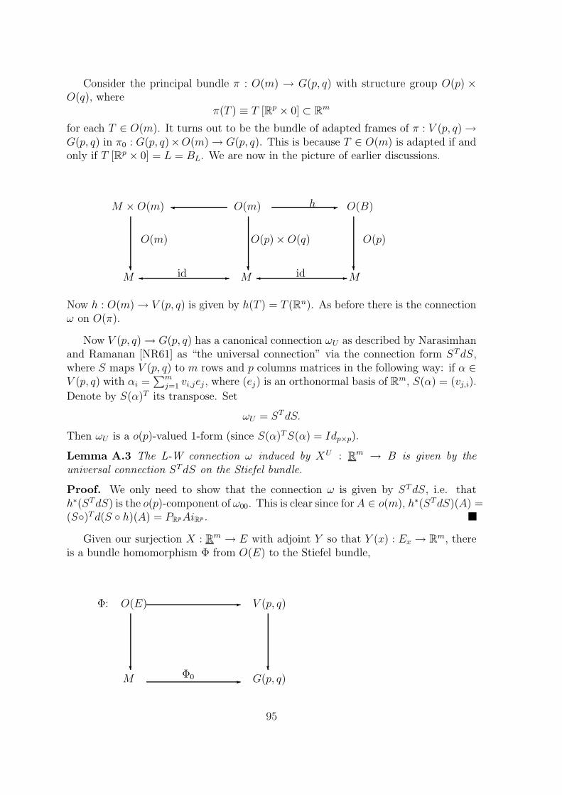
Consider the principal bundle π : O(m) → G(p, q) with structure group O(p) ×O(q), where

π(T ) ≡ T [Rp × 0] ⊂ Rm

for each T ∈ O(m). It turns out to be the bundle of adapted frames of π : V (p, q) →G(p, q) in π0 : G(p, q)×O(m) → G(p, q). This is because T ∈ O(m) is adapted if andonly if T [Rp × 0] = L = BL. We are now in the picture of earlier discussions.

M × O(m) O(m) - O(B)h

?

O(m)

M?

M -id

O(p) × O(q)

?

O(p)

M -id

Now h : O(m) → V (p, q) is given by h(T ) = T (Rn). As before there is the connectionω on O(π).

Now V (p, q) → G(p, q) has a canonical connection ωU as described by Narasimhanand Ramanan [NR61] as “the universal connection” via the connection form STdS,where S maps V (p, q) to m rows and p columns matrices in the following way: if α ∈V (p, q) with αi =

∑mj=1 vi,jej, where (ej) is an orthonormal basis of R

m, S(α) = (vj,i).

Denote by S(α)T its transpose. Set

ωU = STdS.

Then ωU is a o(p)-valued 1-form (since S(α)TS(α) = Idp×p).

Lemma A.3 The L-W connection ω induced by XU : Rm → B is given by the

universal connection STdS on the Stiefel bundle.

Proof. We only need to show that the connection ω is given by STdS, i.e. thath∗(STdS) is the o(p)-component of ω00. This is clear since forA ∈ o(m), h∗(STdS)(A) =(S)Td(S h)(A) = PRpAiRp .

Given our surjection X : Rm → E with adjoint Y so that Y (x) : Ex → R

m, thereis a bundle homomorphism Φ from O(E) to the Stiefel bundle,

Φ: O(E) - V (p, q)

?

M?

G(p, q)-Φ0

95

defined by:

Φ0(x) = Image Y (x),

Φ(u) = (Y (x)u(e1), . . . , Y (x)u(ep)) ,

where (ei) is an orthonormal basis for Rp.

Conversely any such bundle homomorphism Φ : O(E) → V (p, q) over Φ0 : M →G(p, q) comes from a surjective map: indeed for x ∈M , take a frame u ∈ O(E) at x,and set

Y (x) = Φ(u) u−1 : TxM → Rm.

This is independent of the choice of u. Here we have used Φ(u) for the inducedtransformation: R

p → Rm. Set X(x) = Y (x)∗.

On the vector bundle level let E1 → M1 and E2 → M2 be two vector bundlesover manifolds and let f be a vector bundle map which is a 1-1 map on fibres overf0 : M1 → M2. Given a vector bundle map X2 : R

m → E2 there is an induced mapX1 : R

m → E1 given by

X1(x)(e) = (f)−1f0(x)X2 (f0(x)) (e).

E1 - E2f

?

M1

?

M2-f0

RmX2

+

This gives E1 an induced metric and makes f an isometry on fibres. Let ΓX2 bethe L-W connection on O(E2) from X2 and ΓX1 be the L-W connection on O(E1)from X1. Let f ∗

(ΓX2

)be the pull back of ΓX2 .

Lemma A.4f ∗(ΓX2)

=(ΓX1

).

Proof. Let Y1 and Y2 be respectively the adjoint ofX1 andX2. Take e ∈ Image(Y1(x)),say e = Y1(ve). We need only to show

(∇Xe1)x = 0.

Here ∇ is the covariant differentiation corresponding to the pulled back connection.Take a curve σ1 ∈ M1 with σ1(0) = x. Let σ1 be the horizontal lift of σ1(·) in theframe bundle of E1, and σ2 the horizontal lift of f0 (σ1(·)). Then

f (σ1(t)) = σ2(t).

96

By definition,

(∇Xe1)x = σ1(0)

d

dt(σ∗(t))

−1Xe1 (σ(t)) |t=0

= f−1 (σ2(0))d

dt(σ2(t))

−1Xe2 (f0(σ(t))) |t=0

The right hand side is zero from the characterization of L-W connections and theobservation that e is in the image of Y2 since e = Y1(x)(ve) = Y2(f0(x)) (f(ve)).

Theorem A.5 Every metric connection on E is a L-W connection for some X :R

m → E, some finite m.

Proof. By Narasimhan and Ramanan, any metric connection form ωg is given byωg = Φ∗(ωU) from some bundle homomorphism Φ : O(E) → V (p, q). Define X, Yfrom Φ as before.

E - Bf

?

M?

G(p, q)-

RmXU

+

Set f = (XUY ). Then Φ is induced by f and so, by lemma A.3, Φ∗(ωU) is the

connection form for f ∗(ΓXU

). By Lemma A.4 f ∗(ΓXU

)= ΓX . So ωg is the connection

form for the L-W connection ΓX .

B Creation and Annihilation operators (notation

for section 2.4)

Let A : V → V be a linear map on an inner product space V and (e1, . . . , en) anorthonormal base for V . There are the operators (dΛ)∗(A) on the space of tensorproducts of ∧∗V , which restricts to ∧pV to give (dΛ)p(A):

(dΛ)p(A) (u1 ∧ . . . ∧ up) =

p∑

1

u1 ∧ . . . ∧ uj−1 ∧ Auj ∧ uj+1 ∧ . . . ∧ up,

and (δ2Λ)∗

defined by:

(δ2Λ)∗A = (dΛ)∗A (dΛ)∗A− (dΛ)∗A2.

97

If φ is a linear map on ∧pV , we define Aφ(v) = φ(Av) and so the last lineartransformations we defined on ∧pV give:

(dΛ)p(A)(φ)(u1, . . . , up) =

p∑

j=1

φ(u1, . . . , Auj, . . . , up),

and for p > 1

(δ2Λ∗)A(φ)(u1, . . . , up) =∑

i6=j

φ(u1, . . . , Aui, . . . , Auj, . . . , up).

And so(δ2Λ∗)A(φ) = (dΛ∗) (dΛ∗)A(φ) − (dΛ∗)A2(φ),

Let a∗j be the ”creation operator”on ∧∗V , a∗jv = ej∧v if (e1, . . . , en) is an orthonor-mal basis for ∧∗V , and aj its adjoint, the ”annihilation operator”. For linear formswe have the corresponding operators: (aj)∗φ(v) = φ(ajv) and (ajφ)(v) = φ(a∗jv). Inparticular ajφ(v) = φ(ej ∧ v) and (aj)∗φ(v) = e∗j ∧ φ .

ThendΛ∗(A) =

∑

i,j

〈Aej, ei〉 a∗iaj. (B.1)

See [CFKS87].

Lemma B.1(δ2Λ)∗A = −

∑

i,j,k,l

〈Aej, ei〉 〈Aek, el〉 a∗i a∗l ajak.

Proof. By (B.1),

(dΛ)∗ (dΛ)∗(A)(−) =∑

i,j

〈Aej, ei〉 a∗i aj ((dΛ)∗(A)(−))

=∑

i,j,k,l

〈Aej, ei〉 〈Aek, el〉 a∗i aja

∗l ak(−)

= −∑

i,j,k,l

〈Aej, ei〉 〈Aek, el〉 a∗i a∗l ajak(−)

+∑

i,j,k

〈Aej, ei〉 〈Aek, ej〉 a∗i ak(−)

The last step comes from the identity aja∗l = −a∗l aj + δjl, as used in [CFKS87].

However

∑

i,j,k

〈Aej, ei〉 〈Aek, ej〉 a∗iak(−) =

∑

i,j,k

⟨A2ek, ei

⟩a∗i ak(−) = (dΛ∗)(A2).

98

Consequently,

(dΛ)∗ (dΛ)∗(A)(−)

= −∑

i,j,k,l

〈Aej, ei〉 〈Aek, el〉 a∗ia∗l ajak(−) + (dΛ)∗(A2)(−),

Corollary B.2 The map (δ2Λ)∗A : V → V can be written as:

(δ2Λ)∗A = −2∑

i<l,j<k

〈Aej ∧ Aek, ei ∧ el〉 a∗ia∗l ajak.

Proof. Note a∗ja∗j = 0. We split the sum in (δ2Λ)∗A into two parts: i < l and

i > l. After rearrangements, we have:

(δ2Λ)∗(A)

= −∑

i<l,1≤k,j≤m

[〈Aej, ei〉 〈Aek, el〉 − 〈Aej, el〉 〈Aek, ei〉] a∗ia∗l ajak

= −∑

i<l,1≤k,j≤m

〈Aej ∧ Aek, ei ∧ el〉 a∗i a∗l ajak

= −2∑

i<l,k<j

〈Aej ∧ Aek, ei ∧ el〉 a∗i a∗l ajak.

There is a similar expression for linear forms from

(dΛ∗A)(φ) =

∑

i,j

φ(〈Aei, ej〉 a∗iaj) =

∑

i,j

〈Aej, ei〉 (ai)∗ajφ :

Corollary B.3 The map (δ2Λ∗)A : ∧∗V ∗ → ∧pV ∗ is given by:

(δ2Λ)∗A(φ) = −

∑

i,j,k,l

〈Aei, ej〉 〈Aek, el〉 (ai)∗(ak)∗ajal φ

= −2∑

i<k,j<l

〈Aei ∧ Aek, ej ∧ el〉 (ai)∗(ak)∗ajal φ.

C Basic formulae

In this section we give some basic formulae for ∇ and T in terms of the defining mapX or the Gaussian field W .

Let W be a mean zero Gaussian field of sections Γ(E) of a vector bundle E, ∇the associated L-W connection, and let 〈, 〉x be the metric on E induced from theGaussian structure, as given in section 1.1C. Recall (1.1.5):

99

∇vU = EW (x)d

dt〈U(σ(t)),W (σ(t))〉σ(t)

∣∣∣∣t=0

v ∈ TxM,U ∈ ΓE, (C.1)

where σ is any C1 smooth curve with σ(0) = v, and also recall the expansionU = EW 〈u,W 〉 for U ∈ Γ(E).

Proposition C.1 1. For any connection ∇ on E,

∇vU = E ∇vW 〈U,W 〉x0+ ∇vU. (C.2)

2. E ∇WW = 0.

3. A connection ∇ on E is adapted to 〈, 〉x if and only for any U ∈ Γ(E) andtangent vector v,

E ∇vW 〈U,W 〉 + EW⟨U, ∇vW

⟩= 0. (C.3)

Proof. Take v ∈ Tx0M and let σ be a C1 smooth curve with σ(0) = v. ExpandingU (σ(t)) in W we see:

∇vU =D

dtEW (σ(t)) 〈U(σ(t)),W (σ(t))〉σ(t)

∣∣∣∣∣t=0

= E ∇vW 〈U,W 〉x0+ EW (x0)

d

dt〈U(σ(t)),W (σ(t))〉

∣∣∣∣t=0

= E ∇vW 〈U,W 〉x0+ ∇vU.

Thus (C.2). Take ∇ = ∇ in (C.2)) to see part (2) (or use the defining property ofProposition 1.1.3).

Next suppose that ∇ is adapted to the metric. Applying ∇v in the second line ofthe earlier calculation, we have

∇vU = E ∇vW 〈U,W 〉 + EW⟨U, ∇vW

⟩+ ∇vU

and thus (C.3).On the other hand (C.3) implies

E

⟨∇vW,U

⟩〈U,W 〉 = 0.

Consequently,

d 〈U, U〉 (v) = 2⟨∇vU, U

⟩(v)

= 2⟨∇vU, U

⟩− 2E

⟨∇vW,U

⟩〈U,W 〉

= 2⟨∇vU, U

⟩,

i.e. ∇ is metric.

100

Corollary C.2 Let ∇ be a connection on a subbundle E of TM . Denote by T andT respectively the torsions for ∇ and ∇. Then for sections U,Z of E with U(x0) = uand Z(x0) = z,

T (z, u) − T (z, u) = EW (x0)⟨u, ∇zW

⟩− EW (x0)

⟨z, ∇uW

⟩(C.4)

= −E 〈W (x0), u〉 ∇zW + E 〈W (x0), z〉 ∇uW (C.5)

and

T (z, u) = [Z, U ](x0) + E[W,Z](x0) 〈W,u〉x0− E[W,U ](x0) 〈W, z〉x0

. (C.6)

Proof. The first formula follows from (1.3.12) and the second from Proposition C.1and (C.5).

Finally we write ∇ in terms of the vector fields Z · as defined by (1.1.1):

Proposition C.3 Let ∇ be a connection on a subbundle E of TM containing E.Then for U ∈ Γ(E) and V ∈ Γ(TM) with U(x0) = u and V (x0) = v,

∇vU = ∇vU − ∇vZu, (C.7)

∇uV = ∇′uV − ∇vZu. (C.8)

Proof. The first identity is just (1.1.3). The second follows from (1.3.1) and (C.7):

∇uV = ∇vU + [U, V ](x0) = ∇vU − ∇vZu + [U, V ](x0) = ∇′uV − ∇vZ

u.

Formulae related to curvatures

First we give a formula for the curvature tensor R in terms of X or W . From this aseries of identities and inequalities relating the quantities of ∇ with those of ∇ areobserved. In particular we give an interpretation of the form T#, derived from torsionT , being closed or co-closed.

A. Let E be a subbundle of TM , R : TM × TM → L(E;E) the curvature tensorfor a metric connection ∇, and W a Gaussian vector field which induces ∇ in thesense of section 1.1.

Proposition C.4 For u ∈ Ex0, and v1, v2 ∈ Tx0M ,

R(v1, v2)(u) = E ∇v1W⟨∇v2W,u

⟩− E ∇v2W

⟨∇v1W,u

⟩. (C.9)

In the metric form,

R(v1, v2)(u) =∑

i

∇v1Xi⟨∇v2X

i, u⟩−∑

i

∇v2Xi⟨∇v1X

i, u⟩. (C.10)

101

Proof. First recall formula (1.3.12) from section 1.3:

∇vU = [V, U ] + E[W,V ] 〈W,U〉 (C.11)

Let U be a horizontal vector field and V, Z vector fields,then

∇Z[∇V U ] = [Z, ∇VU ] + E [W,Z]⟨W, ∇V U

⟩

= [Z, [V, U ]] + E [Z, [W,V ]] 〈W,U〉

+E [W,V ] d 〈W,U〉 (Z(·)) + E[W,Z]⟨W, ∇V U

⟩.

Use Jacobi’s identity twice to obtain

R(Z, V )U := ∇Z∇V U − ∇V ∇ZU − ∇[Z,V ]U

= E [W,V ] d 〈W,U〉 (Z(·))

− [W,Z] d 〈W,U〉 (V (·))

+E

[W,Z]

⟨W, ∇V U

⟩− [W,V ]

⟨W, ∇ZU

⟩.

Take U = Zu and V, Z with V (x0) = v, Z(x0) = z for z, v ∈ Tx0M , and u ∈ Ex0 .Then

R(z, v)u = E

[W,V ]

⟨∇zW,u

⟩− [W,Z]

⟨∇vW,u

⟩

= E

∇zW 〈∇vW,u〉 − ∇vW 〈∇zW,u〉

,

using (1.3.1) and the independence of W (x) and ∇·W |Tx0M .

Consequently for vi ∈ TxM , ui ∈ Ex,

⟨R(v1, v2)u1, u2

⟩= −E

⟨∇v1W ∧ ∇v2W, u1 ∧ u2

⟩Λ2Ex

.

Corollary C.5 Let R : Λ2TM → Λ2E be the curvature operator defined by

〈R(v1 ∧ v2), u1 ∧ u2)〉 = 〈R(v1, v2)u2, u1〉.

ThenR = E ∇·W ∧ ∇·W.

In the metric form,

R =m∑

i=1

∇·Xi ∧ ∇·X

i.

102

Remark: For A : TM ⊕KerX → E the ’shape operator’, defined by

A(u, e) = ∇X(e)(u),

the proposition gives

R(u, v)w = trace A(u,−) 〈A(v,−), w〉 − A(v,−) 〈A(u,−), w〉

which reduces in the gradient case to Gauss’s equation for the curvature of a sub-manifold in R

m (e.g. p. 23 [KN69b]).

B. Let ∇ and ∇0 be two connections on E with D : TM × E → E the bilinearmap defined by :

∇V U = ∇0V U + D(V, U). (C.12)

Their curvature tensors are related by the following formula: for v1, v2 and u in Ex,

R(v1, v2)u = R0(v1, v2)u+(∇0

v1D)

(v2, u) −(∇0

v2D)

(v1, u)

+D(v1, D(v2, u)) − D(v2, D(v1, u)) + D (T 0(v1, v2), u) ,(C.13)

and the two covariant derivatives of D restricted to E × E are related by

(∇v1D

)(v2, u) −

(∇0

v1D)

(v2, u)

= D(v1, D(v2, u)

)− D

(v2, D(v1, u)

)− D

(D(v1, v2), u

), v1, v2, u ∈ Ex0

In the nondegenerate case, we shall take ∇0 = ∇, the Levi-Civita connection forthe induced metric. Recall the differential 3-form T# defined in section 2.2.

Proposition C.6 Let ∇ be a torsion skew symmetric connection on TM . If R, Rand R denote respectively the curvature tensors for ∇, ∇ and ∇ then:

R(v1, v2)u = R(v1, v2)u+ 12

(∇v1 T

)(v2, u) −

12

(∇v2 T

)(v1, u)

+14T (v1, T (v2, u)) −

14T (v2, T (v1, u)).

(C.14)

In particular,

1.

Ric(u, v) = Ric(u, v) −1

2δT#(u, v) −

1

4tr⟨T (−, u), T (−, v)

⟩, (C.15)

so Ric(−,−) is symmetric if and only if δT# = 0.

2.Ric(u, v) − Ric(u, v) = −δT#(u, v). (C.16)

3.R(v1, v2)u = R(v1, v2)u−

(∇v1 T

)(v2, u) +

(∇v2 T

)(v1, u). (C.17)

103

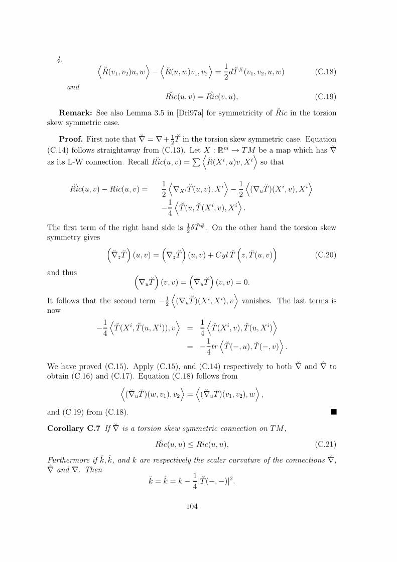
4. ⟨R(v1, v2)u, w

⟩−⟨R(u, w)v1, v2

⟩=

1

2dT#(v1, v2, u, w) (C.18)

andRic(u, v) = Ric(v, u), (C.19)

Remark: See also Lemma 3.5 in [Dri97a] for symmetricity of Ric in the torsionskew symmetric case.

Proof. First note that ∇ = ∇+ 12T in the torsion skew symmetric case. Equation

(C.14) follows straightaway from (C.13). Let X : Rm → TM be a map which has ∇

as its L-W connection. Recall Ric(u, v) =∑⟨

R(X i, u)v,X i⟩

so that

Ric(u, v) − Ric(u, v) =1

2

⟨∇XiT (u, v), X i

⟩−

1

2

⟨(∇uT )(X i, v), X i

⟩

−1

4

⟨T (u, T (X i, v), X i

⟩.

The first term of the right hand side is 12δT#. On the other hand the torsion skew

symmetry gives(∇zT

)(u, v) =

(∇zT

)(u, v) + Cyl T

(z, T (u, v)

)(C.20)

and thus (∇uT

)(v, v) =

(∇uT

)(v, v) = 0.

It follows that the second term − 12

⟨(∇uT )(X i, X i), v

⟩vanishes. The last terms is

now

−1

4

⟨T (X i, T (u,X i)), v

⟩=

1

4

⟨T (X i, v), T (u,X i)

⟩

= −1

4tr⟨T (−, u), T (−, v)

⟩.

We have proved (C.15). Apply (C.15), and (C.14) respectively to both ∇ and ∇ toobtain (C.16) and (C.17). Equation (C.18) follows from

⟨(∇uT )(w, v1), v2

⟩=⟨(∇uT )(v1, v2), w

⟩,

and (C.19) from (C.18).

Corollary C.7 If ∇ is a torsion skew symmetric connection on TM ,

Ric(u, u) ≤ Ric(u, u), (C.21)

Furthermore if k, k, and k are respectively the scaler curvature of the connections ∇,∇ and ∇. Then

k = k = k −1

4|T (−,−)|2.

104

Remarks:(i) When M is a Lie group with ∇ the left invariant connection and 〈, 〉 is bi-

invariant then R ≡ 0, ∇T ≡ 0 and (C.14) reduces to the standard formula for thecurvature

R(v1, v2)u = −1

4[ [Zv1 , Zv2 ], Zu ]

by (1.3.6) and the Jacobi identity.In this case (C.18) shows that T# is a closed form, as is well known: for non-

Abelian compact Lie groups it represents a non-trivial class in H3(G), [Car36], whichis clear since (C.16) shows it is harmonic. Indeed we obtain the following:

if M is compact with dimM ≥ 3 and admits a torsion skew symmetric con-nection with nonzero torsion which is flat together with its adjoint connection thenH3(M ; R) 6= 0.

This would be an extension of Cartan’s result if the existence of such a connectionwere known on any manifolds other than Lie groups.

(ii) The inequality (C.21) does not hold in general without the assumption of tor-sion skew symmetry, even when ∇ is adapted to some metric. A class of counterexamples is provided by Lie groups with left invariant metrics having negative curva-ture, e.g. see [Mil76].

105

D List of notation

M basic manifold,

H Hilbert space, =Rm if finite dimensional

X(x) bundle homomorphism between the trivial bundle M ×H and E over M ,

Y (x) = X(x)∗ : TxM → H,

N(x) = KerX(x) (often aasume of constant rank);

Zv = X(·)Y (x0)v, v ∈ Tx0M

〈, 〉 or 〈, 〉X metric induced on E from X,

〈, 〉1 a Riemannian metric on TM = E ⊕ E⊥, extending the metric induced

on E by X, having E⊥ orthogonal to E

〈, 〉′ a Riemannian metric not necessarily coming from X;

∇, the connection associated to X, R, Ric, Rq its curvature, Ricci

curvature and Weitzenbock terms, and T its torsion tensor

∇ the adjoint semi-connection of ∇, R, Ric, Rq, its curvature, Ricci

curvature, Weitzenbock terms and T its torsion tensor,

∇ Levi-Civita connection, R, Ric, Rq, its curvature, Ricci curvature,

and Weitzenbock terms

∇1 = ∇ ⊕ ∇⊥, the direct sum connection of ∇ on E and a connection

∇⊥ on E⊥, T 1 its torsion

∇ any connection, R its curvature tensor, Ric its Ricci curvature, Rq

its Weitzenbock terms, //· the corresponding parallel

translation, T its torsion tensor, Rijkl the associated curvatures,

Ric#(v) =

m∑

1

Ric(v,X i(x))X i(x),

T# the 3-form related to T ,

W Gaussian field of sections of E,

D (2,0)-tensor, the difference between two linear connections,

A,Aq infinitesimal generator associated with a given sde and its

restriction on q-forms,

Pt semigroup associated with stochastic flows;

AX =1

2

m∑

j

∇Xj(Xj) + A,where A the drift coefficient of the s.d.e. involved,

δ ’divergence’ operator associated to ∇,

ai, (ai)∗ annihilation and creation operator,

ξt(x0), ρ(x0) solution to sde with initial point x0 and life time ρ(x0),

xt = ξt(x0),

106

Tξt the derivative process associated to ξt,

vt often Tx0ξt(v0); for v0 ∈ Tx0M ,

W q,At the solution to covariant equation (3.3.11) involving Rq

βt, Bt orthogonal decomposition of the Brownian motion Bt

on Rm using ∇//

−1

t dBt = dβt + Bt,

Bt = X(x0)Bt, the martingale part of the stochastic anti-development of

ξt(x0)

dEf the restriction of df to E

DiffM C∞ diffeomorphisms of M .

107

Bibliography

[AA96] L. Accardi and Mohari A. On the structure of classical and quantumnflows. J. Funct. Anal., 135(2):421–455, 1996.

[AE95] S. Aida and K.D. Elworthy. Differential calculus on path and loop spaces.1. Logarithmic Sobolev inequalities on path spaces. C. R. Acad. Sci. Paris,t. 321, serie I, pages 97–102, 1995.

[Aid96] S. Aida. Logarithmic Sobolev inequalities on loop spaces over compactRiemannian manifolds. In Stochastic analysis and applications (Powys,1995), pages 1–19. World Sci. Publishing, River Edge, NJ, 1996.

[Aid97] S. Aida. On the irreducibility of certain Dirichlet forms on loop spacesover compact homogeneous spaces. In K. D. Elworthy, S. Kusuoka, andI. Shigekawa, editors, New Trends in stochastic Analysis, Proc. TaniguchiSymposium, Sept. 1995, Charingworth. World Scientific Press, 1997.

[AM95] H. Airault and P. Malliavin. Semi-martingales with values in a Euclideanvector bundle and Ocone’s formula on a Riemannian manifold. Proc.Symp. Pure Maths., 57:175–192, 1995.

[Ama85] S.-I. Amari. Differential-geometrical methods in statistics, volume 28 ofLecture Notes in Statistics. Springer-Verlag, New York, 1985.

[Bak97] D. Bakry. On Sobolev and logarithmic Sobolev inequalities for Markovsemigroups. In K. D. Elworthy, S. Kusuoka, and I. Shigekawa, editors,New Trends in stochastic Analysis’, Proc. Taniguchi Symposium, Sept.1995, Charingworth. World Scientific Press, 1997.

[Bax76] P. Baxendale. Gaussian measures on function spaces. Amer. J. Math.,98:892–952, 1976.

[Bax84] P. Baxendale. Brownian motions in the diffeomorphism groups I. Com-positio Math., 53:19–50, 1984.

[Bax86] P. Baxendale. Asymptotic behaviour of stochastic flows of diffeomor-phisms: two case studies. Probab. Theory Rel. Fields, 73:51–85, 1986.

[Bax81] P. Baxendale. Wiener processes on manifolds of maps. Proc. Roy. Soc.Edinburgh Sect. A, 87(1-2):127–152, 1980/81.

108

[Bel87] Denis R. Bell. The Malliavin Calculus. Longman Scientific & Technical,1987.

[BH86] P. Baxendale and Theodore E. Harris. Isotropic stochastic flows. Ann.Probab., 14(4):1155–1179, 1986.

[Bis81] J. M. Bismut. A generalized formula of Ito and some other properties ofsolution flows. Z. Wahrscheinlichkeitstheorie Verw. Gebiete, 55:331–350,1981.

[Bis84] J. M. Bismut. Large deviations and the Malliavin calculus. Progress inMath. 45. Birkhauser, 1984.

[BR95] V. Bogachev and M. Roeckner. Regularity of invariant measures on finiteand infinite dimensional spaces and applications. J. Funct. Anal., 133:168–223, 1995.

[BS88] P. Baxendale and D.W. Stroock. Large deviations and stochastic flows ofdiffeomorphisms. Prob. Th. Rel. Fields, 81:169–554, 1988.

[Car36] E. Cartan. La Topologie des Espaces Representatives des Groupes de Lie.Hermann, Paris, 1936.

[Car85] A. Carverhill. A formula for the Lyapunov numbers of a stochastic flow:Application to a perturbation theorem. Stochastics, 14:209–226, 1985.

[Car88] A. Carverhill. Conditioning a lifted stochastic system in a product space.The Annals of Probab., 16(4):1840–1853, 1988.

[CE83] A. Carverhill and K. D. Elworthy. Flows of stochastic dynamical systems:the functional analytic approach. Z. Wahrscheinlichkeitstheorie Verw. Ge-biete, 65:245–267, 1983.

[CFKS87] H. Cycon, R. Froese, W. Kirsch, and J. Simon. Schroedinger operatorswith applications to quantum mechanics and global geometry. Texts andMonographs in Physics. Springer-Verlag, 1987.

[CHL] M. Capitaine, E. P. Hsu, and M. Ledoux. Martingale representation and asimple proof of Logarithmic Sobolev inequalities on path spaces. Preprint.

[CM] A.-B. Cruzeiro and P. Malliavin. Curvatures of path spaces and stochasticanalysis. Institut Mittag-Leffler preprints No. 16, 1994/95.

[Dar92] R. W. R. Darling. Isotropic stochastic flows: a survey. In Diffusion pro-cesses and related problems in analysis, Vol. II (Charlotte, NC, 1990),volume 27 of Progr. Probab., pages 75–94. Birkhauser Boston, Boston,MA, 1992.

109

[DPZ92] G. Da Prato and J. Zabczyk. Stochastic Equations in Infinite Dimen-sions. Encyclopedia of Mathematics and its Applications 44, CambridgeUniversity Press, Cambridge., 1992.

[Dri92] B. Driver. A Cameron-Martin type quasi-invariance theorem for Brownianmotion on a compact Riemannian manifold. J. Funct. Anal., 100:272–377,1992.

[Dri95] B. Driver. Towards calculus and geometry on path spaces. In Mark A. Pin-sky Michael C. Cranston, editor, Stochastic Analysis: AMS Proceedings ofsymposium in pure Math. Series, pages 423–426. AMS. Providence, RhodeIsland, 1995.

[Dri97a] B. Driver. Integration by parts for heat kernel measures revisited. J.Math. pures et appl, 76:703–737, 1997.

[Dri97b] B. Driver. The Lie bracket of adapted vector fields on Wiener spaces. Toappear: Applied Math. and Optimization, 1997.

[EL94] K. D. Elworthy and Xue-Mei Li. Formulae for the derivatives of heatsemigroups. J. Funct. Anal., 125(1):252–286, 1994.

[EL96] K. D. Elworthy and Xue-Mei Li. A class of integration by parts formulae instochastic analysis I. In S. Watanabe, editor, Ito’s Stochastic Calculus andProbability Theory (dedicated to Prof. Ito on the occasion of his eightiethbirthday). Springer-Verlag, 1996.

[Eli67] H. Eliasson. Geometry of manifolds of maps. J. Diff. Geom., 1:169–194,1967.

[ELJL97a] K. D. Elworthy, Y. Le Jan, and Xue-Mei Li. Concerning the geometry ofstochastic differential equations and stochastic flows. In K.D. Elworthy,S. Kusuoka, and I. Shigekawa, editors, New Trends in stochastic Analysis’,Proc. Taniguchi Symposium, Sept. 1995, Charingworth. World ScientificPress, 1997.

[ELJL97b] K. D. Elworthy, Y. Le Jan, and Xue-Mei Li. Integration by parts formu-lae for degenerate diffusion measures on path spaces and diffeomorphismgroups. C.R. Acad. Sci. Paris, t. 323 serie 1:921–926, 1997.

[Elw82] K.D. Elworthy. Stochastic Differential Equations on Manifolds. LectureNotes Series 70, Cambridge University Press, 1982.

[Elw88] K. D. Elworthy. Geometric aspects of diffusions on manifolds. In P. L.Hennequin, editor, Ecole d’Ete de Probabilites de Saint-Flour XV-XVII,1985-1987. Lecture Notes in Mathematics, volume 1362, pages 276–425.Springer-Verlag, 1988.

110

[Elw92] K. D. Elworthy. Stochastic flows on Riemannian manifolds. In M. A.Pinsky and V. Wihstutz, editors, Diffusion processes and related problemsin analysis, volume II. Birkhauser Progress in Probability, pages 37–72.Birkhauser, Boston, 1992.

[EM] K.D. Elworthy and Z. Ma. Vector fields on mapping spaces and relatedDirichlet forms and diffusions. Osaka J. Math.

[Eme89] M. Emery. Stochastic Calculus in Manifolds. Springer-Verlag, 1989.

[ER88] K. D. Elworthy and S. Rosenberg. Generalized Bochner theorems and thespectrum of complete manifolds. Acta Appl. Math., 12:1–33, 1988.

[ER91] K.D. Elworthy and S. Rosenberg. Manifolds with wells of negative curva-ture. Invent. Math., 103:471–495, 1991.

[ER96] K. D. Elworthy and S. Rosenberg. Homotopy and homology vanishingtheorems and the stability of stochastic flows. Geometric and FunctionalAnalysis, 6:51–78, 1996.

[ET70] K.D. Elworthy and A. J. Tromba. Differential structures and Fredholmmaps on Banach manifolds. In S.S. Chern and S. Smale, editors, Proc.of Symp. in Pure Maths., XV. Global Analysis. American MathematicalSociety, 1970.

[EY93] K. D. Elworthy and M. Yor. Conditional expectations for derivativesof certain stochastic flows. In J. Azema, P.A. Meyer, and M. Yor, edi-tors, Sem. de Prob. XXVII. Lecture Notes in Maths. 1557, pages 159–172.Springer-Verlag, 1993.

[Har81] Theodore E. Harris. Brownian motions on the homeomorphisms of theplane. Ann. Probab., 9(2):232–254, 1981.

[HL93] R. Harvey and B. Lawson. A theory of characteristic curves associatedwith a singular connection, Asterisque, 213. Societe Mathematique deFrance, 1993.

[Hsu] P. Hsu. Analysis on path and loop spaces. To appear in AMS/Park CityMathematical Series, Vol. 5, edited by E. P. Hsu and S. R. S. Varadhan,American Mathematical Society and Institute for Advanced Study.

[U95] A. S. Ustunel. An introduction to analysis on Wiener space. Lecture Notesin Maths 1610. Springer, 1995.

[IW89] N. Ikeda and S. Watanabe. Stochastic Differential Equations and DiffusionProcesses , second edition. North-Holland, 1989.

[Jan85] Y. Le Jan. On isotropic Brownian motions. Z. WahrscheinlichkeitstheorieVerw. Gebiete, 70:609–620, 1985.

111

[Kif88] Y. Kifer. A note on integrability of cr-norms of stochastic flows and ap-plications. In Stochastic Mechanics and Stochastic Processes (Swansea,1986), Lecture Notes in Math., 1325, pages 125–131. Springer, Berlin-NewYork, 1988.

[KN69a] S. Kobayashi and K. Nomizu. Foundations of differential geometry, Vol.I. Interscience Publishers, 1969.

[KN69b] S. Kobayashi and K. Nomizu. Foundations of differential geometry, Vol.II. Interscience Publishers, 1969.

[Kun80] H. Kunita. On the decomposition of solutions of differential equations. InD. Williams, editor, Stochastic integrals, Lecture Notes in Mathematics,volume 851, pages 213–255, 1980.

[Kun90] H. Kunita. Stochastic Flows and Stochastic Differential Equations. Cam-bridge University Press, 1990.

[Kus88] S Kusuoka. Degree theorem in certain Wiener Riemannian manifolds. InM. Metivier and S. Watanabe, editors, Stochastic Analysis: Proceedings,Paris 1987. Lecture Notes in Maths, 1322, pages 93–108. Springer-Verlag,1988.

[Lea] R. Leandre. Cover of the Brownian bridge and stochastic symplectic ac-tion. Les Prepublications de l’institut Elie Cartan, 96/no 1.

[Li92] Xue-Mei Li. Stochastic Flows on Noncompact Manifolds. Ph.D. thesis,University of Warwick., 1992.

[Li94a] Xue-Mei Li. Stochastic differential equations on noncompact manifolds:moment stability and its topological consequences. Probab. Theory Relat.Fields, 100(4):417–428, 1994.

[Li94b] Xue-Mei Li. Strong p-completeness and the existence of smooth flowson noncompact manifolds. Probab. Theory Relat. Fields, 100(4):485–511,1994.

[LJW84] Y. Le Jan and S. Watanabe. Stochastic flows of diffeomorphisms. In K. Ito,editor, Proc. of Taniguchi Symp. Katata, 1982. Stochastic Analysis, pages307–332. North Holland, 1984.

[Lon] H.-W. Long. Symmetric diffusion operators on infinite dimensional spaces.Ph. D. thesis, Warwick, 1997.

[Mal91] P. Malliavin. Stochastic Analysis, Grundlehren der math. Wiss., volume313. Springer, 1991.

[Mil76] J. Milnor. Curvatures of left invariant metrics on Lie groups. Advances inMath, 21:293–329, 1976.

112

[Nor86] J. Norris. Simplified Malliavin calculus. In J. Azema and M. Yor, editors,Seminaire de Probability XX. Lecture Notes in Mathematics, 1204, pages101–130. Springer-Verlag, 1986.

[NR61] M.S. Narasimhan and S. Ramanan. Existence of universal connections.American J. Math., 83, 1961.

[PVB96] Fernand Pelletier and Liane Valere Bouche. The problem of geodesics, in-trinsic derivation and the use of control theory in singular sub-Riemanniangeometry. In Actes de la Table Ronde de Geometrie Differentielle (Lu-miny, 1992), volume 1 of Semin. Congr., pages 453–512. Soc. Math.France, Paris, 1996.

[Ros97] Steven Rosenberg. The Laplacian on a Riemannian manifold, volume 31 ofLondon Mathematical Society Student Texts. Cambridge University Press,Cambridge, 1997. An introduction to analysis on manifolds.

[RS80] M. Reed and B. Simon. Methods of modern mathematical physics, vol-ume II. Academic Press, 1980.

[RY91] D. Revuz and M. Yor. Continuous martingales and Brownian motion.Springer-Verlag, 1991.

[Str86] Robert S. Strichartz. Sub-Riemannian geometry. J. Differential geometry,24:221–261, 1986.

[SZ96] D. W. Stroock and O. Zeitouni. Variations on a theme by Bismut.Asterisque, (236):291–301, 1996. Hommage a P. A. Meyer et J. Neveu.

[TW96] A. Thalmaier and W.-Y. Wang. Gradient estimates for harmonic functionson regular domains in Riemannian manifolds. To appear J. Funct. Anal.,1996.

113