ON THE FOUNDATIONS OF MATHEMATICSmat.msgsu.edu.tr/~dpierce/Courses/111/2005/Notes/notes.pdf · x3...
178
INTRODUCTORY NOTES ON THE FOUNDATIONS OF MATHEMATICS
Transcript of ON THE FOUNDATIONS OF MATHEMATICSmat.msgsu.edu.tr/~dpierce/Courses/111/2005/Notes/notes.pdf · x3...

INTRODUCTORY NOTES
ON THE FOUNDATIONS OF MATHEMATICS

Introductory Notes
on the
Foundations of Mathematics
David Pierce
September 14, 2005

Preface
These notes concern the foundations of mathematics in two ways:
(∗) these notes are about concepts and techniques that all mathematiciansuse, implicitly or explicitly;
(†) these notes (or parts of them) are intended for use in a first university-levelmathematics course.
More precisely, these notes are originally written for a course called Fundamen-tals of Mathematics, given at Middle East Technical University in Ankara underthe designation Math 111.1 The notes also offer additional reading for those in-terested in the topics they discuss. In particular, the notes may be useful forMath 320 (Set Theory) and Math 406 (Introduction to Mathematical Logic andModel Theory) at METU.
What are foundations? A wooden house may by built on a stone foundation.A mason lays down the stones; then a carpenter erects the house on top. Thecarpenter cannot construct the walls and floors of the house before the stone-mason creates a place to set those floors and walls; but the stone-mason cannotcreate this foundation without knowing what the carpenter intends to placethere.
So it is with the foundations of mathematics. You cannot do mathematics with-out a place to start; but you cannot create the starting-point without knowingthe mathematics that will proceed from it. This is a paradox—a seeming con-tradiction. It is not a real contradiction; but it does suggest that the nascentmathematician (the first-year student) cannot read these notes page after pageas if they constituted an easy novel. They might constitute a difficult novel withlots of interrelated events. (However, not every novel has an index or a list ofsymbols like this one.) Not every section of these notes should be studied in se-quence during the reader’s first encounter. Even if an earlier section is requiredfor a later section, still, that earlier section may not be fully comprehensiblewithout some knowledge of the later section.
What can the reader do? Read slowly, but jump ahead; reread what you havealready read; think the whole time, but do not think too much without really
1The catalogue description of Math 111 is:
Symbolic logic. Set theory. Cartesian product. Relations. Functions. Injective,surjective and bijective functions. Composition of functions. Equipotent sets.Countability of sets. More about relations: equivalence relations, equivalenceclasses and partitions. Quotient sets. Order relations: Partial order, Total order,Well ordering. Mathematical induction and recursive definitions of functions.
i

ii
knowing what you are thinking about. Talk to classmates; talk to teachers.Read with a pencil. Summarize passages in your own words. Invent yourown symbolism (while remembering that communicating with others requires acommon symbolism). Read other books on the same subjects.
Also: do exercises. Create your own exercises. Most sections of these notes endwith exercises. The student who is in a hurry will find out from a teacher whichexercises to work on and will then try to do them immediately, looking back intothe sections as necessary for examples. A difficulty in this approach is that mostexercises here do not have unique correct answers; they have solutions, someof which are better than others. Finding the best solutions—even acceptablesolutions—will require reading, thinking, and experience. Still, many of theexercises can be approached as puzzles: they do not need deep insight into thenature of things, but aim only to develop facility with some basic ideas.
Most exercises here could not very well be cast as multiple-choice questions. Ina multiple-choice question, if you can somehow figure out the correct answer,even without being able to say how you did it, your answer is still 100% correct.Here, correct solutions to problems will carry within themselves the reasons whythey are correct.
There are no answers at the back of the book. Problems here can have more thanone correct solution; you should be able to tell whether a particular solution iscorrect. It is true that you may fail to notice some mistakes; the only way toavoid this is experience, not desire or will.
Somebody who does not know a language very well will not avoid mistakes justby trying hard: s/he2 must practice. Likewise with games: even if you memorizeall of the moves of chess and think real hard, you will not play a good chess-game at first. Depending on how seriously you take mathematics, you can seethese notes as lessons in a language or a game.
It would be worthwhile for the reader to have a look at Euclid’s Elements.(Heath’s English translation from the Greek is [14]—see the bibliography atthe end of these notes. This translation is available in print and in variousplaces around the Web.) The present notes do not share much content with theElements; but Euclid’s work does establish a sort of foundation or prototypefor the mathematics of his and all succeeding generations, including our own.
Euclid wrote the Elements, the original textbook of mathematics, some 2300years ago.3 This textbook is still in use in some classrooms today. It consistsof 13 books. You are not likely to read all of them; as with the present work,you will jump around, reading what you are interested in, perhaps with theguidance of a teacher. Indeed, probably Euclid expected few people to read his
2The construction s/he can be pronounced as she or he (or as he or she). English has notevolved a generally accepted singular pronoun that refers to humans of either sex: it lacksthe o(n) of Turkish. In the fourteenth century, according to the OED [28], the second-personplural pronoun you began to be used respectfully in place of the singular pronoun thou, just asthe Turkish siz replaces sen. In the same way, currently, some people use they with a singularsense. Other people are bothered by this usage, and they may insist that he can refer tohumans of unknown sex. The original OED does not recognize this usage, although it doesclaim that she comes from a different base than he, because the feminine form derived fromthe base of he was too much like the masculine form.
3Euclid practiced mathematics in Alexandria around 300 bce, probably having learnedmathematics in Athens from the students of Plato [14, vol. I, pp. 1 f.].
iii
work unaided. His work does bring the reader instantly into real mathematics;but it also sets a standard for spareness of mathematical composition.
The Elements contains no commentary, no guidance for the reader. After afew definitions and axioms, the work consists solely of propositions and theirproof s. Euclid doesn’t tell you, but he shows you what proofs of propositionsare.
The present notes contain more than just propositions and their proofs; but theydo contain these. Each proof here is labelled as such, and ends with a little box.(The first example is on p. 9.) The propositions and proofs in these notes consistof sentences of ordinary language, with some abbreviative symbolism (as wellas the symbolism required by what the proofs are about). Such proofs might becalled informal, because ordinary language is itself informal. Grammatical rulesfor English or Turkish or any other human language can indeed be formulated,and the conscientious speaker or writer will try to follow them; but it seemsimpossible to formulate grammatical rules that are obeyed by everything thatone wants to say.
Informal proofs are to be distinguished from formal proofs (or deductions).Again, the notion of proof itself—informal proof—is over two thousand yearsold; but the notion of a formal proof dates only from the 1920s.4 These notestell you, as well as show you, what formal proofs are. Briefly described, a formalproof is a list of sentences of an artificial language; but such a list must satisfycertain requirements. The last sentence on the list is what the formal proofis a proof of : it is what the proof proves. A machine could check whether agiven list of sentences is a formal proof. To establish the truth of an interestingproposition, a formal proof is practically never called for. However, if it is heldto the highest standard, an informal proof of some proposition P can be seenas an argument that a formal proof of P could in principle be written.
It will be an exercise in these notes to write some formal proofs; but the ultimategoal is the ability to check the validity of informal proofs (like Euclid’s, or anylater mathematician’s), and the ability to write one’s own (informal) proofs.
I assume that you, the reader, have some experience with high-school algebra,and specifically with the algebra of the integers. Then you can prove an identitylike
x3 + y3 = (x+ y)(x2 − xy + y2) (0.1)
(by multiplying out the right member and combining like terms). The algebraof the integers serves as a pattern for Boolean algebra, which I shall introduceas the algebra of the numbers 0 and 1 alone. If one considers these numbersto represent falsity and truth, then Boolean algebra determines an algebra ofpropositions, or a propositional logic.
After we have propositional logic, we can say something about predicate logic.This logic provides for the analysis of propositions into parts, some of whichare not propositions. (Some parts of propositions will be predicates: hence thename of the logic.) We can’t define everything precisely until we have the notionof a relation. Relations are certain sets; they are subsets of Cartesian productsof sets. So all of these things will need to be discussed.
4Perhaps the invention can be attributed to Hilbert [7, §07, n. 110].
iv
A function can be defined as a kind of relation. Functions give us a way to saywhen two sets ‘have the same size,’ or are equipollent (or ‘equipotent’). The setof integers has the same size as the set of even integers; both sets are countablyinfinite; but there are strictly larger, uncountable sets, such as the set of realnumbers.
The predicate logic given here is more precisely called first-order predicate logic.Functions also allow us to give an account of first-order logic in general.
The integers have an ordering. This is a kind of relation. There is a generaliza-tion called a partial ordering . We shall prove a representation theorem, namelythe proposition that every partial ordering behaves like the subset-relation (ina clearly defined way).
Equality is also a relation and is the motivating example of an equivalence-relation. The standard sorts of numbers—integers, rational numbers, realnumbers, complex numbers—can be formally defined in terms of equivalence-relations, once one has the natural numbers 0, 1, 2, 3, . . . The idea of these notesis that we do not really have these numbers, mathematically, until we can givea logical account of them. These notes end with such an account.
The topics of these notes are so interrelated that in any discussion of them, itis hard to avoid the appearance of circularity. This circularity is a part of thefoundational aspect of these notes. As I say, I assume that the reader is familiarwith the integers; but I also say that we do not officially have the integersuntil the end of the notes. Yet my supposedly rigorous account of the integersdepends on all of the machinery that the notes develop first, with the aid of afamiliarity with. . . the integers.
Our path will have been, not circular, but spiral or rather helical, as if along awinding staircase. We start from the integers, and then we return to them, butat a higher (or deeper) level than where we started.
Typography
These printed words are assembled by means of the collection of typesettingprograms and packages known as AMS-LATEX. Here, TEX is in Greek letters5;the same three letters will appear below, in § 1.0, in the full Greek name oflogic. In the Latin alphabet, the letters are written tech, as in technical. TheAMS is the American Mathematical Society. The original TEX program wasexpanded into LATEX and independently into AMS-TEX; then the benefits ofboth expansions were combined into AMS-LATEX.
The original TEX program distinguishes between ordinary text and mathemat-ical text. In ordinary text, in these notes, words are italicized for the usualsorts of reasons: they (or rather their meanings) are being emphasized, they aretitles, they are not in the language of the surrounding text, and so forth. I amalso making some further distinctions. Technical terms are in bold-face whenthey are being defined, explicitly or implicitly. Technical terms might simplybe slanted if their precise definitions will come later or are simply not needed.
5See [24, p. 1].
v
Words that are being talked about or mentioned (and not simply being used)6
are in sanserif. However, I may not have always been consistent in making thesedistinctions.
Footnotes here are intended to contain only material that is not essential to themain point. They may contain historical information that I have happened todiscover, although much of the history of what I am discussing is still unknownto me. Footnotes may also contain forward references.
The LATEX program provides an easy way to make numbered lists. So as not tohave too many numerals around, I often replace the usual list
1 2 3 4 5 6 7 8 9
with the alternative
∗ † ‡ § ¶ ‖ ∗∗ †† ‡‡
that is provided in LATEX. Another reason to use these symbols7 is to avoid thesuggestion of ranking. I may start numbered lists with 0 instead of 1.
Labelled proofs here end with boxes, as noted above; labelled examples end withbullets (the first is on p. 31).
Acknowledgments
In these notes, some of the material on logic and numbers was first preparedby me in 2001; at the same time, Andreas Tiefenbach prepared notes on setsand relations. Andreas, Belgin Korkmaz, and I taught Math 111 from thosenotes. Andreas and I revised our respective notes, with Belgin’s advice, thefollowing year. In 2004, in preparing to teach Math 111 that fall along withAyse Berkman and Mahmut Kuzucuoglu, I composed my own complete setof notes, drawing on Andreas’s notes in giving my own account of sets andrelations. Now, at the beginning of 2005, I am revising the notes again, keepingin mind the experience of Ayse, Mahmut and myself, along with impressionsfrom students. Advice from my friend Steve Thomas is also proving useful forthis revision.
Many of the topics dealt with in these notes are also covered by basic texts like[13] or [34]. I am not trying to write such a book as these are, but I find it usefulto look at them. The preface of [34] is particularly reassuring, as it describesthe many changes that the authors have made in each new edition of their book.
6The distinction between the use and the mention of a word (or symbol) is attributedto Quine in [7, § 08, p. 61]. The sentence ‘A woman or a man is a human’ uses the wordwoman. The sentence ‘The English word for kadın also has five letters’ mentions the wordwoman without using it. The sentence ‘Woman has five letters’ uses the word woman tomention the same word. Such a use can be called autonymous, following Carnap: again,the attribution is in [7, § 08, p. 61], where it is said that Frege introduced the practice ofindicating autonymous use of words by quotation-marks (inverted commas). By this practice,the last quoted sentence would be “ ‘Woman’ has five letters.”
7In the order given, the first five symbols are an asterisk, a dagger, a double dagger, asection-sign, and a pilcrow.
vi
My own notes on logic draw from various sources, especially [7] and [5]; AliNesin’s book [29] is an account in Turkish of some of the same material.
Set-theory on the level of my coverage seems generally to be found only inmore advanced texts like [41] or [26]. I use these books, but try to give moreelementary exercises than they do.
For my notes on natural numbers, [25] is inspirational.
As a student, I appreciated the style of Spivak [39]: not condescending, buttreating the reader as a fellow mathematician.
Thanks to Sukru Yalcınkaya and Vural Cam for the photographic representa-tions of the digits 1 and 0 on the cover; the pictures were made at Perge and atTermessos; the column at Perge is in the Corinthian order.
Open Your Own Treasure House
Daiju visited the master Baso in China. Baso asked: “What do youseek?”
“Enlightenment,” replied Daiju.
“You have your own treasure house. Why do you search outside?”Baso asked.
Daiju inquired: “Where is my treasure house?”
Baso answered: “What you are asking is your treasure house.”
Daiju was enlightened! Ever after he urged his friends: “Open yourown treasure house and use those treasures.” [33, p. 55]

Contents
List of Figures ix
1 Introduction 1
1.0 Logic . . . . . . . . . . . . . . . . . . . . . . . . . . . . . . . . . . 1
1.1 Language and propositions . . . . . . . . . . . . . . . . . . . . . 2
1.2 Classes, sets, and numbers . . . . . . . . . . . . . . . . . . . . . . 7
1.3 Algebra of the integers . . . . . . . . . . . . . . . . . . . . . . . . 13
1.4 Some proofs . . . . . . . . . . . . . . . . . . . . . . . . . . . . . . 19
1.5 Excursus on anthyphaeresis . . . . . . . . . . . . . . . . . . . . . 23
1.6 Parity . . . . . . . . . . . . . . . . . . . . . . . . . . . . . . . . . 26
1.7 Boolean connectives . . . . . . . . . . . . . . . . . . . . . . . . . 29
1.8 Propositional formulas and language . . . . . . . . . . . . . . . . 32
1.9 Quantifiers . . . . . . . . . . . . . . . . . . . . . . . . . . . . . . 35
2 Propositional logic 41
2.0 Truth-tables . . . . . . . . . . . . . . . . . . . . . . . . . . . . . . 41
2.1 Unique readability . . . . . . . . . . . . . . . . . . . . . . . . . . 46
2.2 Truth-equivalence . . . . . . . . . . . . . . . . . . . . . . . . . . . 50
2.3 Substitution and replacement . . . . . . . . . . . . . . . . . . . . 52
2.4 Normal forms . . . . . . . . . . . . . . . . . . . . . . . . . . . . . 55
2.5 Adequacy . . . . . . . . . . . . . . . . . . . . . . . . . . . . . . . 58
2.6 Simplification . . . . . . . . . . . . . . . . . . . . . . . . . . . . . 61
2.7 Logical consequence and formal proofs . . . . . . . . . . . . . . . 64
2.8 Proof-systems . . . . . . . . . . . . . . . . . . . . . . . . . . . . . 68
2.9 ÃLukasiewicz’s proof system . . . . . . . . . . . . . . . . . . . . . 70
vii

viii CONTENTS
3 Sets and Relations 74
3.0 Boolean operations on sets . . . . . . . . . . . . . . . . . . . . . . 74
3.1 Inclusions and implications . . . . . . . . . . . . . . . . . . . . . 81
3.2 Cartesian products, and relations . . . . . . . . . . . . . . . . . . 85
3.3 Functions . . . . . . . . . . . . . . . . . . . . . . . . . . . . . . . 90
3.4 Deeper into functions . . . . . . . . . . . . . . . . . . . . . . . . . 94
3.5 First-order logic . . . . . . . . . . . . . . . . . . . . . . . . . . . . 98
3.6 Equipollence . . . . . . . . . . . . . . . . . . . . . . . . . . . . . 108
3.7 Equivalence-relations . . . . . . . . . . . . . . . . . . . . . . . . . 110
3.8 Orderings . . . . . . . . . . . . . . . . . . . . . . . . . . . . . . . 113
3.9 Infinitary Boolean operations . . . . . . . . . . . . . . . . . . . . 118
4 Numbers 120
4.0 The Peano axioms . . . . . . . . . . . . . . . . . . . . . . . . . . 120
4.1 Recursion . . . . . . . . . . . . . . . . . . . . . . . . . . . . . . . 122
4.2 The arithmetic operations . . . . . . . . . . . . . . . . . . . . . . 125
4.3 The integers and the rational numbers . . . . . . . . . . . . . . . 127
4.4 Recursion generalized . . . . . . . . . . . . . . . . . . . . . . . . 130
4.5 The ordering of the natural numbers . . . . . . . . . . . . . . . . 131
4.6 The real numbers . . . . . . . . . . . . . . . . . . . . . . . . . . . 134
4.7 Well-ordered sets . . . . . . . . . . . . . . . . . . . . . . . . . . . 135
4.8 Cardinality . . . . . . . . . . . . . . . . . . . . . . . . . . . . . . 141
4.9 Uncountable sets . . . . . . . . . . . . . . . . . . . . . . . . . . . 146
A Aristotle’s Analytics 148
Bibliography 151
Symbols 155
Index 157
List of Figures
1.1 The Greek alphabet . . . . . . . . . . . . . . . . . . . . . . . . . 2
1.2 Logical adjectives . . . . . . . . . . . . . . . . . . . . . . . . . . . 36
3.1 Venn diagrams of combinations of sets . . . . . . . . . . . . . . . 75
3.2 Cartesian product . . . . . . . . . . . . . . . . . . . . . . . . . . 85
3.3 The less-than relation on Z . . . . . . . . . . . . . . . . . . . . . 88
3.4 Converse of a relation . . . . . . . . . . . . . . . . . . . . . . . . 96
3.5 Diagonal on a set . . . . . . . . . . . . . . . . . . . . . . . . . . . 97
3.6 Projection . . . . . . . . . . . . . . . . . . . . . . . . . . . . . . . 103
3.7 The temple at Assos: the Doric order . . . . . . . . . . . . . . . 114
3.8 A partial order of propositional formulas . . . . . . . . . . . . . . 115
3.9 Two isomorphic partial orders: . . . . . . . . . . . . . . . . . . . 117
3.10 A partial order of sets . . . . . . . . . . . . . . . . . . . . . . . . 118
4.1 Functions used in the proof of Theorem 4.8.1. . . . . . . . . . . . 142
ix

Chapter 1
Introduction
1.0 Logic
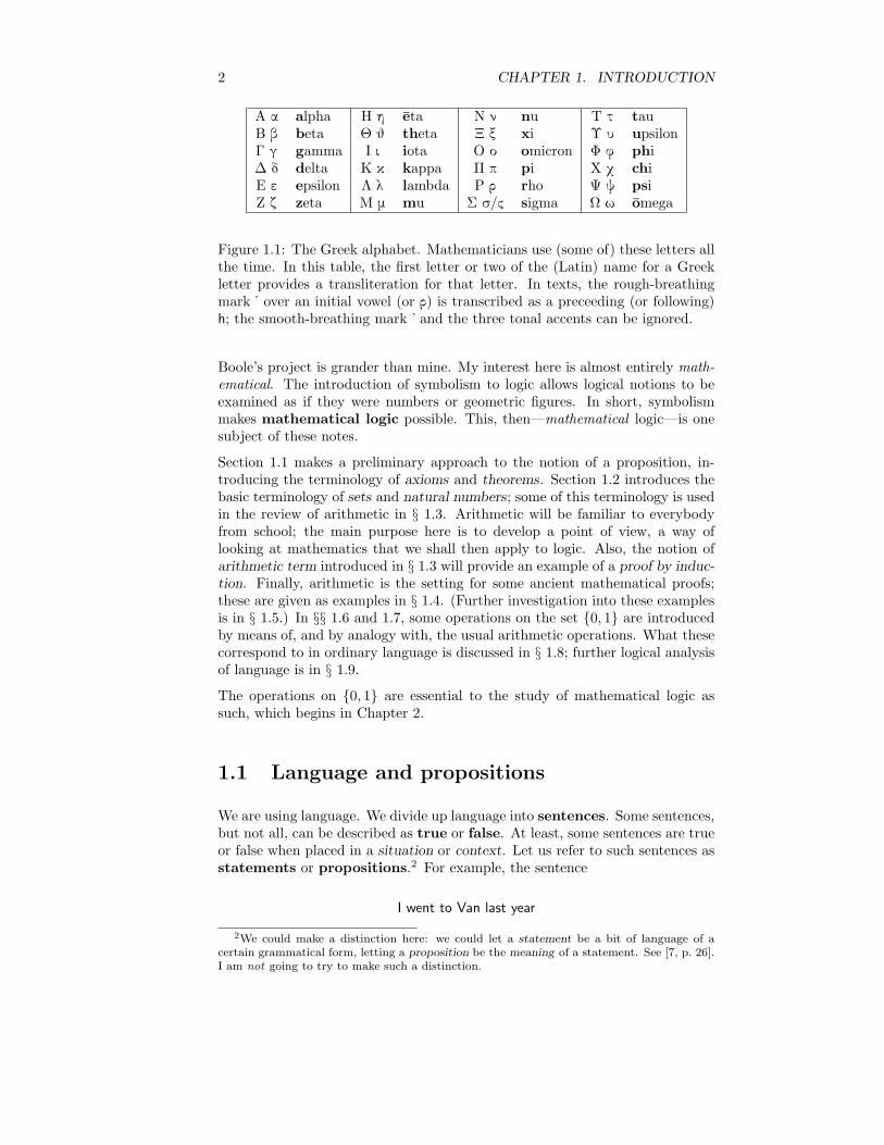
The name of logic comes ultimately from the (ancient) Greek adjective lογική,which is short for lογικ τέχνη. This phrase can be rendered in English as therational art, or the art of reason. I shall not attempt to define reason. In Latinletters, the Greek phrase is he logike techne. But knowing the Greek alphabet isworthwhile, if only because mathematicians use it as a source of symbols. SeeFigure 1.1 below.
Logic as a field of study can be counted as a part of philosophy . One can dologic with ordinary language alone. Aristotle (384–322 bce [3, pp. vii–ix]) isclassically considered the originator of logic, and his texts are in ordinary Greek,albeit with some use of (Greek) letters to stand for parts of sentences. I shalltake him as a source for some fundamental ideas: see §§ 1.1 and 1.8, as well asAppendix A.
Symbolic logic consciously develops a special notation for the notions thatlogic examines. Some two thousand years after Aristotle, George Boole describesthe process at the beginning of The Laws of Thought [4, [1], p. 1], first publishedin 1854:
The design of the following treatise is to investigate the fundamentallaws of those operations of the mind by which reasoning is performed;to give expression to them in the symbolic language of a Calculus,1
and upon this foundation to establish the science of Logic and con-struct its method; to make the method itself the basis of a generalmethod for the application of the mathematical doctrine of Prob-abilities; and, finally, to collect from the various elements of truthbrought to view in the course of these inquiries some probable inti-mations concerning the nature and constitution of the human mind.
1This is calculus in the sense of a method of calculating; it has little to do with theinfinitesimal calculus, which is the subject now called just calculus. What is referred to inthese notes as propositional logic can also be called propositional calculus.
1
2 CHAPTER 1. INTRODUCTION
Α α alpha Η η eta Ν ν nu Τ τ tauΒ β beta Θ θ theta X ξ xi Υ υ upsilonΓ γ gamma Ι ι iota Ο ο omicron Φ φ phi∆ δ delta Κ κ kappa Π π pi Χ χ chiΕ ε epsilon L l lambda Ρ ρ rho Ψ ψ psiΖ ζ zeta Μ µ mu Σ σv/c sigma Ω ω omega
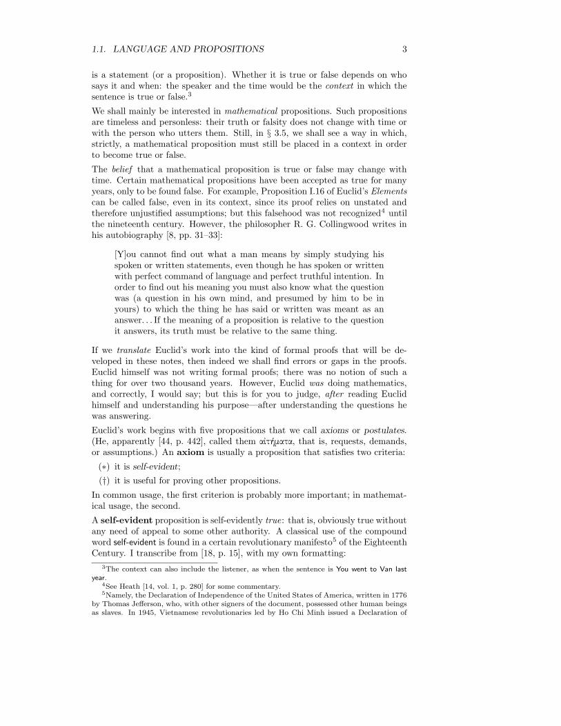
Figure 1.1: The Greek alphabet. Mathematicians use (some of) these letters allthe time. In this table, the first letter or two of the (Latin) name for a Greekletter provides a transliteration for that letter. In texts, the rough-breathingmark < over an initial vowel (or ρ) is transcribed as a preceeding (or following)h; the smooth-breathing mark > and the three tonal accents can be ignored.
Boole’s project is grander than mine. My interest here is almost entirely math-ematical. The introduction of symbolism to logic allows logical notions to beexamined as if they were numbers or geometric figures. In short, symbolismmakes mathematical logic possible. This, then—mathematical logic—is onesubject of these notes.
Section 1.1 makes a preliminary approach to the notion of a proposition, in-troducing the terminology of axioms and theorems. Section 1.2 introduces thebasic terminology of sets and natural numbers; some of this terminology is usedin the review of arithmetic in § 1.3. Arithmetic will be familiar to everybodyfrom school; the main purpose here is to develop a point of view, a way oflooking at mathematics that we shall then apply to logic. Also, the notion ofarithmetic term introduced in § 1.3 will provide an example of a proof by induc-tion. Finally, arithmetic is the setting for some ancient mathematical proofs;these are given as examples in § 1.4. (Further investigation into these examplesis in § 1.5.) In §§ 1.6 and 1.7, some operations on the set 0, 1 are introducedby means of, and by analogy with, the usual arithmetic operations. What thesecorrespond to in ordinary language is discussed in § 1.8; further logical analysisof language is in § 1.9.The operations on 0, 1 are essential to the study of mathematical logic assuch, which begins in Chapter 2.
1.1 Language and propositions
We are using language. We divide up language into sentences. Some sentences,but not all, can be described as true or false. At least, some sentences are trueor false when placed in a situation or context. Let us refer to such sentences asstatements or propositions.2 For example, the sentence
I went to Van last year
2We could make a distinction here: we could let a statement be a bit of language of acertain grammatical form, letting a proposition be the meaning of a statement. See [7, p. 26].I am not going to try to make such a distinction.
1.1. LANGUAGE AND PROPOSITIONS 3
is a statement (or a proposition). Whether it is true or false depends on whosays it and when: the speaker and the time would be the context in which thesentence is true or false.3
We shall mainly be interested in mathematical propositions. Such propositionsare timeless and personless: their truth or falsity does not change with time orwith the person who utters them. Still, in § 3.5, we shall see a way in which,strictly, a mathematical proposition must still be placed in a context in orderto become true or false.
The belief that a mathematical proposition is true or false may change withtime. Certain mathematical propositions have been accepted as true for manyyears, only to be found false. For example, Proposition I.16 of Euclid’s Elementscan be called false, even in its context, since its proof relies on unstated andtherefore unjustified assumptions; but this falsehood was not recognized4 untilthe nineteenth century. However, the philosopher R. G. Collingwood writes inhis autobiography [8, pp. 31–33]:
[Y]ou cannot find out what a man means by simply studying hisspoken or written statements, even though he has spoken or writtenwith perfect command of language and perfect truthful intention. Inorder to find out his meaning you must also know what the questionwas (a question in his own mind, and presumed by him to be inyours) to which the thing he has said or written was meant as ananswer. . . If the meaning of a proposition is relative to the questionit answers, its truth must be relative to the same thing.
If we translate Euclid’s work into the kind of formal proofs that will be de-veloped in these notes, then indeed we shall find errors or gaps in the proofs.Euclid himself was not writing formal proofs; there was no notion of such athing for over two thousand years. However, Euclid was doing mathematics,and correctly, I would say; but this is for you to judge, after reading Euclidhimself and understanding his purpose—after understanding the questions hewas answering.
Euclid’s work begins with five propositions that we call axioms or postulates.(He, apparently [44, p. 442], called them αÊτήµατα, that is, requests, demands,or assumptions.) An axiom is usually a proposition that satisfies two criteria:
(∗) it is self-evident;
(†) it is useful for proving other propositions.
In common usage, the first criterion is probably more important; in mathemat-ical usage, the second.
A self-evident proposition is self-evidently true: that is, obviously true withoutany need of appeal to some other authority. A classical use of the compoundword self-evident is found in a certain revolutionary manifesto5 of the EighteenthCentury. I transcribe from [18, p. 15], with my own formatting:
3The context can also include the listener, as when the sentence is You went to Van lastyear.
4See Heath [14, vol. 1, p. 280] for some commentary.5Namely, the Declaration of Independence of the United States of America, written in 1776
by Thomas Jefferson, who, with other signers of the document, possessed other human beingsas slaves. In 1945, Vietnamese revolutionaries led by Ho Chi Minh issued a Declaration of

4 CHAPTER 1. INTRODUCTION
We hold these truths to be self-evident,
(∗) that all men are created equal,
(†) that they are endowed by their Creator with certain unalienablerights,
(‡) that among these are life, liberty and the pursuit of happiness.
(§) That to secure these rights, governments are instituted amongmen, deriving their just powers from the consent of the gov-erned.
(¶) That whenever any form of government becomes destructive ofthese ends, it is the right of the people to alter or abolish it,and to institute new government, laying its foundation on suchprinciples and organizing its powers in such form, as to themshall seem most likely to effect their safety and happiness.
Two thousand years earlier, before Euclid even, in the collection of books nowknown as the Metaphysics [3], Aristotle writes of axioms, using the Greek sourceof our word axiom, namely ξιώµα. This word has the root meaning of somethingworthy, or an honor. Aristotle seems to use axiom almost as a synonym ofprinciple (ρχή) or common notion (κοιν δόξα). His writing is elliptical, in thestyle of lecture-notes—which is probably just what his works are [3, pp. xxv &xxxi]; I translate accordingly below, with seemingly missing words supplied inbrackets. (Some of the original Greek words in parentheses are the sources ofmodern technical terms.)
In Book Β of the Metaphysics, Aristotle introduces some questions:
Yet indeed, concerning the demonstrative (ποδεικτικόc) principles,whether they belong to one science (âπιστήµη) or more (πlειών) isdebatable. I call demonstrative the common notions from which ev-erybody proves (δείκνυµι) [propositions], for example, it is necessaryto affirm or deny everything6, or it is impossible to be and not beat the same time7, and however many other such premisses.
These so-called common notions are discussed further in Book Γ, which openswith a statement of the general subject, which we call metaphysics, but Aris-totle called first philosophy:
[1003 a 20] There is a science (âπιστήµη) that looks at (θεωρει) beingas such (τä ïν îν) and what applies to it (τ τούτú Íπάρχοντα)according to itself (καθ αÍτό).8
Independence that enunciated some of the truths of the American declaration [50, ch. 18]; thisdid not prevent a later American invasion.
6pan Ćnagkaion ń fĹnai ń ĆpofĹnai.7ĆdÔnaton Ľma eÚnai kaÈ mŸ eÚnai.8The whole Greek sentence, as given in [3], is ^Estin âpistămh tic ą jewrei tä ïn ŋ în kaÈ tĂ
toÔtú ÍpĹrqonta kajfl aÍtì. The Greek în (stem înt-) is the neuter participle correspondingto the Engish being and the Turkish olan; it appears in modern technical terms like ontology.The feminine stem of the participle is oÖs-; from this is derived the abstract noun oÎsÐa,which I translate below as beingness, although a traditional (and misleading) translation issubstance.
1.1. LANGUAGE AND PROPOSITIONS 5
A Turkish version of this passage, from [1], is
Varlık olmak bakımından varligı ve ona ozu geregi ait olan ana nite-likleri inceleyen bir bilim vardır.
Later in Book Γ, in ch. 3, Aristotle takes up axioms; but he understands them assomething more general than the subject of a particular field like mathematicsor physics. First he seems to repeat the question raised in Book Β:
[1005 a 19] It must be said whether [the inquiry] concerning the so-called axioms (ξιώµατα) of mathematics, and concerning beingness( οÎσία), belongs to one science (âπιστήµη) or another (áτέρα).
It is evident (φανερόν) that the inquiry (σκεψίc) concerning thesebelongs to one [science], namely that of the philosopher (φιlοσόφοc).
For, [the axioms] apply to all beings, not just to some particularclass (γένοc) apart from the others.
Also, all [scientists] use [the axioms]—because they are of being assuch—while each class [has] being.
To whatever extent is appropriate for them, to that extent they use[the axioms]—that is, to the extent of the class concerning whichthey carry out their proofs (ποδείξειc).
So, because it is clear (δηlόν) that [the axioms] apply to all thingsas beings—for this [namely, being] is common to them—the theory(θεωρία) concerning them belongs to those who are gaining knowl-edge (γνωρίζοντοι) concerning being as such.
Therefore, none of those making particular investigations (οÉ κατµέροc âπισκοπούντοι) tries to say something concerning them,—if[they] are true or not—not the geometer (γεωµέτρηc), not the arith-metician (ριθµητικόc).
But some of the physicists (φυσικοι)9 [were] doing this appropriately(εÊκότωc).
For, they thought they alone were doing research (σκοπειν) concern-ing all nature ( φύσιc) and concerning being.
But since there is somebody even higher (νωτέρω) than the physi-cist—for nature is [just] some one class of being—the inquiry con-cerning these would belong to the theoretician (θεωρητικόc) of gen-erality (καθόlου) and first [or primary] beingness ( πρώτη οÎσία).
Physics ( φυσική) is a kind of wisdom (σοφία), but not the first [orforemost] (πρώτη).
Presently we come to what were called common notions in Book Β, then axioms,and now principles:
9Aristotle’s ‘physicists’ are such pre-Socratic philosophers as Thales of Miletus, who arediscussed in Book A of the Metaphysics.

6 CHAPTER 1. INTRODUCTION
[1005 b 8] It is proper for the one who knows best each class [ofthings] to be able to state the most certain principles (ρχαί) of thething (πράγµα):
So that the one [who knows best] being as such [can state] the mostcertain [principles] of all [things]. This is the philosopher.
The most certain principle of all is that about which being mistakenis impossible.
This principle is the Law of Contradiction, which Aristotle now states moreprecisely than in Book Β :
[1005 b 19] For the same [predicate] to apply and not apply at thesame time to the same [subject] in the same [respect] is impossible.10
The grammatical notions of subject and predicate are discussed briefly in § 1.2below. Meanwhile, a Turkish rendition of Aristotle’s formulation of the Law ofContradiction, again from [1], is
Aynı niteligin, aynı zamanda, aynı ozneye, aynı bakımından hem aitolması, hem de olmaması imkansızdır.
After a long discussion of the Law of Contradiction and those who question it,Aristotle gives the Law of the Excluded Middle, again with slightly differentwording from Book Β:
Neither does [any]thing admit to being between a contradiction, butit is necessary either to affirm or deny one of one, whatever.11
Ote yandan celisik onermeler arasında bir aracının olması da imkan-sızdır. Bir ozne hakkında tek bir yuklemi—hangi yuklem olursaolsun—, zorunlu olarak ya tasdik etmek veya inkar etmek gerekir.
The continuation of this passage is in § 1.8. If we follow Aristotle, it seems that,as mathematicians, we need not concern ourselves with the Laws of Contradic-tion and the Excluded Middle; we can just accept these principles and use them;it is the philosopher’s job to identify and enunciate them. But the logician isalso a philosopher. In any case, we shall use these principles explicitly in thenext section; but we shall also see an apparent violation of one of them. Therewe shall also begin to state axioms in our mathematical sense.
A theorem today is usually considered just as a noteworthy proposition witha proof from axioms. The first example is Theorem 1.2.2 in the next section.The word theorem itself comes from the Greek θεώρηµα, and it is related to theverb with the meaning of look at. (This verb is found at the beginning of BookΓ of the Metaphysics as quoted above.) In former times, finer distinctions wereconsidered. Writes Pappus of Alexandria, a few centuries after Aristotle:12
10tä gĂr aÎtä Ľma ÍpĹrqein te kaÈ mŸ ÍpĹrqein ĆdÔnaton tÆ aÎtÆ kaÈ katĂ tä aÎtì.11>AllĂ mŸn oÎdà metaxÌ ĆntifĹsewc ândèqetai eÚnai oÎjèn, Ćllfl ĆnĹgkh ń fĹnai ń ĆpofĹnaiãn kajfl ánäc åtioun.
12Pappus may have been born during the reign of Theodosius I, 379–395 bce, or he mayhave flourished earlier, during the reign of Diocletian, 284–305 bce. The possibilities arediscussed in [45, pp. 564–567], where also are found the text and translation from which thequotation is adapted.

1.2. CLASSES, SETS, AND NUMBERS 7
Those who favor a more technical terminology in geometrical re-search use problem (πρόβlηµα) to mean a [proposition13] in which itis proposed to do or construct [something]; and theorem, a [proposi-tion] in which the consequences and necessary implications of certainhypotheses are investigated; but among the ancients some describedthem all as problems, some as theorems.
A lemma is a proposition proved mainly for the sake of proving other propo-sitions; the first example will be Lemma 1.4.2. (The Greek lέµµα means thatwhich is peeled off, and is from the verb, lέπω, with the meaning of peel.) Acorollary to a theorem is a proposition that follows almost immediately fromthe theorem; the first example will be Corollary 1.4.6.
1.2 Classes, sets, and numbers
In Chapter 3, we shall have a lot to say about sets; but it will be useful to havethe basic notion available from the beginning.
A set is many things, made into one. There are many special cases of sets:Two matching earrings make a pair ; several football-players make a team; thepigeons descending on bread-crumbs in the park make a flock. Words like pair,team and flock are collective nouns. In mathematics, the word set is the mostgeneral collective noun—except for the word class.14
In the previous section, I translated Aristotle’s word γένοc as class, but thatdoes not mean that our understanding will be the same as Aristotle’s. Forus, every set is a class, but not every class is a set. A class is made up ofelements or members. In the context of classes, there is no mathematicaldifference between the words element and member. (However, in an equation,such as (0.1) above or (1.1) below, the expressions on either side of the sign ofequality (that is, =) can be called members of the equation.)
A class is determined by a property. There is no precise definition of property;I shall just say that, for every property, there is a class whose members areprecisely the things that have that property. This does not mean that a class isnecessarily a thing that can itself be a member of classes.
A set is a class that is a member of some classes, though it may fail to be amember of others. If A is a set, and C is a class, then the sentence
A is a member of C
is true or false—it is a proposition. Later in this section, there is an example ofa class that is not a set. (The recognition of a distinction between classes andsets is only about a hundred years old.)
A class can be indicated in writing by braces around its members. So, if wehave, say, three objects,
a, b, c,
13Ivor Thomas [45, p. 567] uses inquiry here; but there is no word in the Greek originalcorresponding to this or proposition.
14One writer [26] seems to use collection more generally even than class.
8 CHAPTER 1. INTRODUCTION
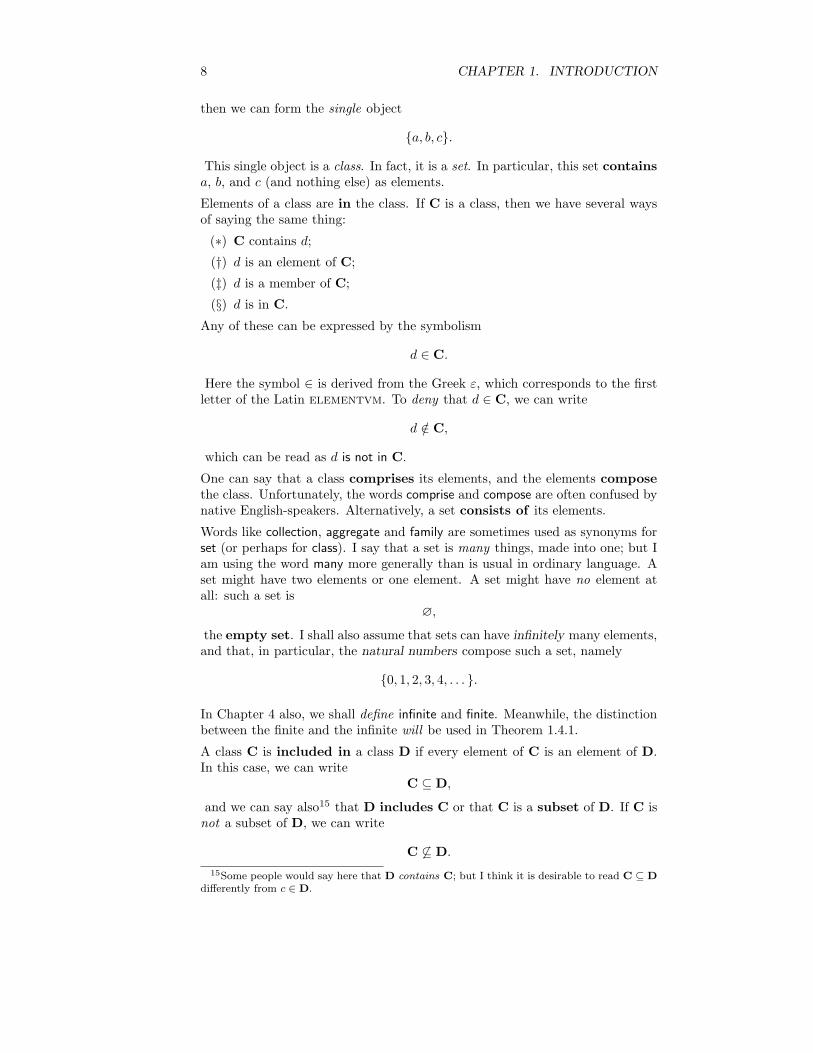
then we can form the single object
a, b, c.
This single object is a class. In fact, it is a set. In particular, this set containsa, b, and c (and nothing else) as elements.
Elements of a class are in the class. If C is a class, then we have several waysof saying the same thing:
(∗) C contains d;
(†) d is an element of C;
(‡) d is a member of C;
(§) d is in C.
Any of these can be expressed by the symbolism
d ∈ C.
Here the symbol ∈ is derived from the Greek ε, which corresponds to the firstletter of the Latin elementvm. To deny that d ∈ C, we can write
d /∈ C,
which can be read as d is not in C.
One can say that a class comprises its elements, and the elements composethe class. Unfortunately, the words comprise and compose are often confused bynative English-speakers. Alternatively, a set consists of its elements.
Words like collection, aggregate and family are sometimes used as synonyms forset (or perhaps for class). I say that a set is many things, made into one; but Iam using the word many more generally than is usual in ordinary language. Aset might have two elements or one element. A set might have no element atall: such a set is
∅,
the empty set. I shall also assume that sets can have infinitely many elements,and that, in particular, the natural numbers compose such a set, namely
0, 1, 2, 3, 4, . . . .
In Chapter 4 also, we shall define infinite and finite. Meanwhile, the distinctionbetween the finite and the infinite will be used in Theorem 1.4.1.
A class C is included in a class D if every element of C is an element of D.In this case, we can write
C ⊆ D,
and we can say also15 that D includes C or that C is a subset of D. If C isnot a subset of D, we can write
C 6⊆ D.
15Some people would say here that D contains C; but I think it is desirable to read C ⊆ Ddifferently from c ∈ D.

1.2. CLASSES, SETS, AND NUMBERS 9
The first axiom of set-theory is that sets are determined by their elements, sothat if two sets have the same elements, then the sets themselves are the same,that is, equal. We can express this more symbolically:
1.2.1 Axiom (Extension). If A and B are sets such that A ⊆ B and B ⊆ A,then
A = B. (1.1)
Instead of A ⊆ B, some people write
A ⊂ B;
but I prefer to use this to mean that A is a proper subset of B: that is, A ⊆ B,but A 6= B.
I say above that a class is determined by a property. A property can be sym-bolized by a predicate. A predicate ‘says something’ about a subject. (See theLaw of Contradiction, in the previous section, as translated from Aristotle.) IfP is a predicate, then the corresponding class can be denoted
x : Px; (1.2)
this is read as the class of x such that P [applies to] x; here, the variable x takesthe place of a grammatical subject of P .
Often, in place of Px, we have to write something that features x more thanonce. For example, there is a property of not being a member of oneself. Inwords, the corresponding predicate is something like
is not a member of -self, (1.3)
with two spaces left for a subject. The phrase is not a member of is also sym-bolized by /∈; so the given property determines the class
x : x /∈ x. (1.4)
This is the historically first16 example of a class that is not a set:
1.2.2 Theorem. The class x : x /∈ x is not a set.
Proof. Call this classR, and suppose it is a set. ThenR is a member of itself, ornot, by the Law of the Excluded Middle, because by definition, sets are the sortsof things that can be members of classes. If R ∈ R, then this very proposition(R ∈ R) shows that R fails to have the defining property of members of R,and so R /∈ R. In short, if R ∈ R, then R /∈ R. Therefore R /∈ R. Thisproposition (R /∈ R) means R does have the defining property of members ofR, so R ∈ R. Thus R is and is not a member of itself, which violates the Lawof Contradiction. Therefore the assumption that R is a set must be mistaken,so R is not a set (by the Law of the Excluded Middle).
16From 1903; see for example [26, I.2.3, p. 6], where both Russell and Zermelo are attributed.

10 CHAPTER 1. INTRODUCTION
The proof ends with a box,17 as noted on p. iii. The proof shows that there is aclass to which the predicate in Line (1.3) neither applies nor fails to apply. Sothere is a violation of the Law of the Excluded Middle—or rather, there is anexample of a class that is not a real thing.
A way to avoid creating classes that are not sets is the following. Suppose U issome set, and P is a predicate. Another axiom18 of set-theory is that the classof elements of U with the property symbolized by P is a set:
1.2.3 Axiom (Separation). The class x ∈ U : Px is a set.
The letter U here stands for universe; but the set could be anything. For amundane example, we could let U be the set of human beings living now, andlet P be is over two meters tall. Then x ∈ U : Px is the set of people nowtaller than two meters.
Mathematical examples of sets of the form x ∈ U : Px will come up through-out these notes.
In the mathematical study of sets, it turns out that there is no need to considerclasses that contain anything other than sets. Here is why:
If A and B are sets, then they have a union, which is the set comprising everyelement of A or B (or both); this union is denoted
A ∪B.
(See § 3.0.) We do have one set, namely the empty set. If A is a set, then wesuppose that we can form the set
A,
which contains only A. Such a set, with a unique element, is called a singleton.(See § 3.2.) Hence, from any set A, we can form the union
A ∪ A;
this is the (set-theoretic) successor of A and can be denoted
A′.
This idea of successsors can be used to give the following inductive definitionof the natural numbers:
First, we declare that the number zero is just the empty set:
0 = ∅.
Then we define the natural numbers by two rules:
(∗) 0 is a natural number;
(†) if n is a natural number and is a set, then n′ is a natural number.
17Other writers use a different symbol, or none at all. An old-fashioned termination of aproof is qed, for the Latin qvod erat demonstrandvm, with the meaning of which was tobe demonstrated.
18The following Axiom of Separation is also called the Axiom of Comprehension.

1.2. CLASSES, SETS, AND NUMBERS 11
If n is a set, then n′ is a set. Hence, every natural number obtained by one ofthe two rules is a set. Therefore, all natural numbers are sets, and every naturalnumber has a successor, which is a natural number.
The definition of the natural numbers is inductive, because it allows proof byinduction in the following sense. Suppose P names a possible property ofnatural numbers, and:
(∗) P0;(†) if Pn, then P (n′), for every natural number n.
Then every natural number must have the property (named by) P . Here, Pn isthe inductive hypothesis. The method of proof by induction is first usedin Lemma 1.2.5 below. In general, an inductive proof consists of two steps:
(∗) the base step, in which P0 is proved;
(†) the inductive step, in which P (n′) is proved from the inductive hypoth-esis Pn.
It is perhaps not obvious that there is even a class consisting of the naturalnumbers: what property do these numbers share? Well, they share the propertythat they can be obtained by starting with ∅ and taking successors. The classof natural numbers is then denoted
ω.
Note well that this symbol is not a w, a double u; it is an omega. To rememberthis, observe that mega means big, so an omega is a big o—rather, a double o,or oo, which, if written quickly, may come out looking like ω.
As we have just defined them, the natural numbers can be called more preciselythe von-Neumann19 natural numbers. The first five von-Neumann naturalnumbers are:
0, 0, 0, 0, 0, 0, 0, 0, 0, 0, 0, 0, 0, 0, 0, 0.
We have the following standard symbols for some successors:
n 0 1 2 3 4 5 6 7 8n′ 1 2 3 4 5 6 7 8 9
Also, we may writen+ 1
for n′. If m and n are in ω, and m ⊆ n, then we usually write
m 6 n.
The class ω has two more properties, besides being inductive: these are givenby the next two theorems:
1.2.4 Theorem. 0 is not the successor of any natural number.
Proof. By definition, every successor of a natural number contains that number;but 0 is empty.
19In fact, the definition is traced to Zermelo in 1916 in [26, II.3.8, p. 54].
12 CHAPTER 1. INTRODUCTION
1.2.5 Lemma. Every von-Neumann natural number includes all of its elements.
Proof. Let P be the predicate
includes all of its elements.
Since 0 has no elements, it includes all of its elements, so P0. This completesthe base step of our proof.
For the inductive step, suppose Pn (as an inductive hypothesis). Say k ∈ n′.Since n′ = n ∪ n, either k ∈ n, or k ∈ n. If k ∈ n, then k ⊆ n by inductivehypothesis. If k ∈ n, then k = n, so k ⊆ n. In either case, k ⊆ n. But n ⊆ n′.Hence k ⊆ n′. (This conclusion will be part of Lemma 3.1.3.) Therefore P (n′).This completes the induction.
1.2.6 Theorem. Natural numbers with the same successor are the same.
Proof. Suppose k and n are natural numbers, and k′ = n′. Then
k ∪ k = n ∪ n.
In particular, k ∈ n ∪ n and n ∈ k ∪ k. If k = n, we are done. If k 6= n,then we must have k ∈ n and n ∈ k, hence k ⊆ n and n ⊆ k by the previouslemma, and therefore k = n by the Axiom of Extension, 1.2.1.
We can call n the immediate predecessor of n′. If n is a natural numberdifferent from 0, then n itself has an immediate predecessor; we have just shownthat this predecessor is unique, and we can denote it by
n− 1.
The von-Neumann definition of the natural numbers is convenient, becauseaccording to this definition, each natural number n is just the set that can bedenoted
0, . . . , n− 1.(If n = 0, then this is the empty set.) If we do not happen to care about whethereach natural number is such a set, then we can denote the set of natural numbersby
N;
this is the usual notation when one is not that interested in set-theory. ThenN is just a class that contains an element 0, and whose every element n has asuccessor, which can be denoted
n+ (1.5)
or n+ 1, such that:
(∗) 0 is not the successor of any element of N;
(†) elements of N with the same successor are the same;
(‡) N is included in every class that contains 0 and that contains n+ if itcontains some n in N.
We shall show in Chapter 4 that all properties of N follow from these.

1.3. ALGEBRA OF THE INTEGERS 13
1.3 Algebra of the integers
Now that we have, in the previous section, a precise definition of the naturalnumbers, I want to review some things we know about them from school. Wecannot yet define all of these things precisely, or prove them: this will happenin Chapter 4. Meanwhile, we just have the set N, whose members form the list
(0, 1, 2, 3, . . . ).
As we have seen, every natural number n has a successor, which usually denotedn+1. Some mathematicians start the list of natural numbers at 1 instead of 0;but I shall just say that the members of the set 1, 2, 3, . . . are the positivenatural numbers.
The number 0 does not have an immediate predecessor that is a natural number;but it does have the immediate predecessor called −1. This is not a naturalnumber, but it is an integer. The set of integers comprises every naturalnumber, along with a negative, denoted −n, for each positive natural numbern. Then −n has the successor −(n−1) and the immediate predecessor −(n+1).The integers that are not natural numbers are also called negative integers.Every integer n has a negative, denoted −n, although this number is itselfnegative only if n is positive.
The set of integers is commonly denoted20
Z.
This set is equipped with three operations, namely addition, additive inver-sion, and multiplication. (Operations are functions; functions in general andoperations in particular are defined formally in § 3.3.) In particular, if x and yare integers, then so are
(∗) x+ y (the sum of x and y, which here are addends),
(†) −x (minus-x, the additive inverse or negative of x), and
(‡) x · y (the product of the factors x and y).
By convention, multiplication is also indicated by juxtaposition; that is, theproduct x · y is also denoted
xy.
Something like the symbol for additive inversion is also used for a fourth op-eration, subtraction, which can be defined in terms of the other operations.
20Here the letter zed or zee stands for the German Zahl, number. In English, the integers arealso called whole numbers. In fact, the English word integer comes from the Latin integer,which means whole. This Latin word developed in France into the French word entier, whichentered English and became entire. Thus two English words—integer and entire—representthe same Latin word. People interested in such matters may refer to such pairs of words asdoublets.

14 CHAPTER 1. INTRODUCTION
Subtracting21 y from x produces a difference, which is denoted
x− y
and which is just the sum of x and −y. Note that x − y is not generally thesame as y− x. If we want to assign names, then, in the difference x− y, we cancall x the minuend (from the Latin, with the meaning of that which is to bediminished), and we can call y the subtrahend (that which is to be subtracted).
Subtraction is thus a composition of two other operations. The process ofcomputing x− y can be indicated by a tree,22 thus:
x y
/.-,()*+−ÄÄÄÄ
/.-,()*++
/////////ÄÄÄÄÄ
More complicated compositions and trees are possible. For example, the tree
x y z w
/.-,()*+−ÄÄÄÄ /.-,()*++
?????ÄÄÄÄÄ
ÂÁÀ¿»¼½¾·
OOOOOOOOO
ooooooooo
/.-,()*++
*************
jjjjjjjjjjjjj
indicates the sum of x and the product of minus-y and the sum of z and w.Usually this sum is written on one line, as
x+−y · (z + w). (1.6)
I shall refer to such a string of symbols as an arithmetic term23 (The Greekword24 for number is ριθµόc, which is arithmos in Latin letters. Our generaldefinition25 of term comes in § 3.5.)Officially, arithmetic terms will be certain strings composed of
• the symbols +, − and · (a dot);
21The English verb subtract is sometimes pronounced as if it were substract. The Englishverb comes from a participle of the Latin verb whose infinitive is subtrahere. This verb is inturn built up from trahere (meaning draw or carry) and the preposition sub (meaning frombelow or away). According to the OED [28], in medieval times, an s was inserted between sub
and trahere, yielding substrahere, from which came substract in English; but this formationis considered incorrect. The English word abstract is from the Latin abstrahere, but herethe s belongs properly to the preposition abs, although the preposition is more commonlyseen as ab or even a.
22Trees as such are covered in a later course, Math 112.23Here the word arithmetic is an adjective and is pronounced with the stress on the penul-
timate (next-to-last) syllable.24Strictly, the Greek word Ćrijmìc refers to a number of things, in particular, more than
one;—certainly not zero or ‘fewer’ than zero. See [22].25In another context, Aristotle’s definition of term is in Appendix A.

1.3. ALGEBRA OF THE INTEGERS 15
• variables, such26 as x, y and z;
• symbols for certain integers, such as 12, 0 and −137—such symbols canbe called numerals27 or (numeral) constants28;
• the parentheses ( and ).
The formal definition of arithmetic terms is inductive, in the sense of the pre-vious section:
(∗) every variable is an arithmetic term;
(†) every numeral is an arithmetic term;
(‡) if t is an arithmetic term, then so is −t;(§) if t0 and t1 are arithmetic terms, then so are (t0 + t1) and (t0 · t1).
Some writers add another condition to this definition:
(¶) nothing else is an arithmetic term.
However, I understand such a condition to be implicit in every inductive defini-tion.
Our definition of arithmetic terms is inductive in the following way. Suppose Ais some set of strings of symbols such that:
(∗) every variable is in A;
(†) every numeral is in A;
(‡) if t is in A, then −t is in A;(§) if t0 and t1 are in A, then so are (t0 + t1) and (t0 · t1).
Then A contains all arithmetic terms. Therefore, proof by induction on arith-metic terms is possible; here is an example:
1.3.1 Proposition. Every arithmetic term has as many left parentheses asright parentheses.
Proof. Let A be the set of arithmetic terms with as many left parentheses asright parentheses. Then A contains all variables and constants (since thesehave no parentheses). Suppose A contains t. Then t has as many left as rightparentheses (just because it is in A), so the same is true of −t. This means −tis in A. Similarly, if t0 and t1 are in A, then each of them has as many left asright parentheses, so the same is true of (t0 + t1) and (t0 · t1); this means theseterms are also in A. By the inductive definition of arithmetic terms, every termis in A.
26The convention of using letters from the end of the Latin alphabet for ‘unknown quantities’dates back to Descartes; see [10]. Since we don’t want any limit on the number of variableswe can use, and yet we want to define things precisely, we could declare officially that ourvariables must come from the list x0, x1, x2 and so forth, except that we can’t preciselyexplain the words and so forth yet.
27It is probably simplest to think of a numeral as a single symbol, even though, typo-graphically, it may be a string of digits, possibly preceeded by a minus-sign. For example,the numeral −137 might be thought of as the single symbol c
−137 (that’s c with the sub-script −137). Our decimal convention for writing numerals is just that, a convention; it hasno essential relation to our definition of arithmetic terms. See also Footnote 31 below.
28Letters from the front of the Latin alphabet are used to denote such constants; again theconvention is found in Descartes. Used in this way, the letters can be called literal constants,where the word literal is just the adjectival form of letter. But for us, literal constants are notliterally parts of terms; they just stand for parts of terms—namely, numerals.
16 CHAPTER 1. INTRODUCTION
By the formal definition of arithmetic terms, the string on Line (1.6) above isnot a term; to satisfy the definition, the term should be written as
(x+ (−y · (z + w))).
By convention, we can leave out the dot between −y and (z + w), and we canremove some of the parentheses. But we can do this only because we have aconventional order of operations in terms. By this convention, expressionsin brackets are evaluated before all else, and then multiplication is performedbefore addition (and subtraction), but otherwise operations are performed asthey are read from left to right. So, (x + y)z means something different fromx+ yz: the former is an informal version of the term ((x+ y) · z); the latter, of(x+ (y · z)).The formal definition of arithmetic terms should ensure that each term indicatesuniquely how to calculate an integer, once integral values are assigned to thevariables. In short, arithmetic terms should be uniquely readable. That ourterms are uniquely readable has a proof like that of Theorem 2.1.4 below.
An arithmetic term is not exactly the same thing as a polynomial. For example,the terms (x · (y + z)) and ((x · y) + (x · z)) are different. However, they alwaysyield the same number if x, y and z are respectively replaced by the same threeintegers. We therefore write
x(y + z) = xy + xz, (1.7)
and we shall say that the two members of this equation represent the samepolynomial. Also, Equation (1.7) is called an (arithmetic) identity.
An equation of arithmetic terms can be called a Diophantine equation, inmemory of the ancient Alexandrian mathematician Diophantus, who studiedsuch equations.29 A Diophantine equation is an example of an (arithmetic)formula. For example, the equation
y2 = 4x3 − ax− b (1.8)
(where a and b are understood to be integers) is an arithmetic formula. Itssolutions are those pairs of integers that satisfy the equation: those pairs(c, d) of integers such that d2 = 4c3 − ac − b. Formula (1.8) is not an identity,because not every pair of integers satisfies it. (For example, if (c, d) and (c, d′)satisfy it, then we must have d′ = ±d; there is no other possibility.)30
By our definition, a polynomial is an abstraction from the notion of a term.It is an equivalence-class of terms, in the sense of § 3.7. You can think of a
29Diophantus wrote the Arithmetica, in thirteen books, of which six have come down to us[45, pp. 516, n. a]. One problem that he considers, for example, is, in our notation, to findrational solutions to the pair
8x + 4 = y2,
6x + 4 = y2
of equations [45, pp. 526–535].30Equations like (1.8) are of ongoing interest to number-theorists. It is a twentieth-century
result that the equation y2 = x3 + 17 has two solutions, (−2, 3) and (2, 5), from which allrational solutions can be found by certain rules; and only eight of these solutions are integral[37, Example III.2.4, pp. 59 f.].
1.3. ALGEBRA OF THE INTEGERS 17
polynomial as an operation. Then a term is a set of instructions—a recipe forhow to perform the operation. The point then is that the same operation canbe performed in different ways. This is why different terms can represent thesame polynomial.
For example, the term x+y says, ‘Start with x, and add y’; the term y+x says,‘To y, add x.’ These are different activities, but they yield the same result; sowe write x+ y = y + x.
How can you tell when two terms represent the same polynomial? It is easy toshow when they represent different polynomials. For example, x2 (that is, xx)represents a different polynomial from x, since (−1)2 6= −1. But how do we knowthat the two members of Equation (1.7) represent the same polynomial? As anidentity, the equation expresses the distributive property of multiplication overaddition. So how do we know that multiplication has this property with respectto addition? We can check it for certain integers, say x = 5 and y = 17 andz = −14:
5(17 +−14) = 5 · 3 = 15;
5 · 17 + 5 · −14 = 85− 70 = 15.
But we can’t check the property for all integers, since there are infinitely many.
Strictly speaking, if one wants to use the distributive property with full un-derstanding, then one should give precise definitions of the integers and theiroperations, and then one should prove the distributive property. We shall beable to do this in Chapter 4: see Theorem 4.2.4. However, we didn’t need toknow all of the properties like the distributive property, just to be able to definethe notion of a polynomial.
As we have discussed them so far, the integers form the structure
(Z,+,−, ·). (1.9)
Structures are defined generally in §§ 3.2 and 3.5. The structure on Line (1.9) isthe set Z equipped with certain specified operations, namely addition, additiveinversion and multiplication. Now, Z also has the named31 elements 0 and 1.Moreover, Z is equipped with the relation < called ‘less-than’. (Relations aredefined generally in § 3.2.) So we may think of the integers as composing thestructure
(Z,+,−, ·, 0, 1, <). (1.10)
We now have some new arithmetic formulas, the simplest being
x < y,
read as x is less than y. There are some ‘derivative’ relations:
• x > y is read as x is greater than y, and means y < x;
• x 6 y means x < y or x = y: that is, x 6 y is satisfied by those (a, b) suchthat a < b or a = b;
31In fact, every integer can be given a name in decimal notation. Alternatively we can justwrite every positive integer as the appropriate sum 1 + 1 + · · ·+ 1, write zero as 0, and writeevery negative integer as −(1 + · · ·+ 1).

18 CHAPTER 1. INTRODUCTION
• x > y is read as x is greater than or equal to y, and means y 6 x.
These are all (arithmetic) inequalities; as such, they are new examples of arith-metic formulas. In general, an inequality is an expression
t0 ∗ t1,
where t0 and t1 are terms, and ∗ is one of the symbols, <, >, 6 and >. In thiscontext, we may also speak of the inequation
t0 6= t1,
which is satisfied by just those integers that do not satisfy the equation t0 = t1.
The positive integers are just the positive natural numbers; symbolically, theseare the integers that satisfy the inequality 0 < x. The negative integers arethose integers that satisfy x < 0. The non-negative integersnon-negative —satisfy 0 6 x and are the natural numbers, composing the set N as we said in§ 1.2.An integer x is a factor or divisor of the integer y if xz = y for some integer z. Inthis case, if x 6= 0, then z is unique; we may then say that z is the quotient y/x.
In general, for any integer y and non-zero integer x, there is a quotient y/x, butthis quotient may only be an element of the set of rational numbers; it maynot be an integer. The set of rational numbers is denoted
Q;
but I prefer to work only with integers for now.
If x is a divisor of y, we writex | y,
and we say that x divides y. So the symbol | denotes a relation, just as <denotes a relation.
A positive integer is called prime if its only positive factors are 1 and itself,and these are distinct. So 1 itself is not prime. A positive integer that is not 1and is not prime is composite. The list of prime numbers begins:
2, 3, 5, 7, 11, 13, 17, 19, 23, 29, 31, 37, 41, 43, 47, 53, 59, 61, 67, 71, 73, 79, 83, 89, 97.
Does the list end? That the list does not end is Proposition IX.20 of Euclid’sElements; we shall give a version of Euclid’s proof in the next section.
Exercises
(1) Is there a way to define arithmetic terms without using brackets? (See § 2.1for some ideas.)
(2) Which of the following equations are arithmetic identities?
(a) xy = yx,
(b) x(yz) = xyz,

1.4. SOME PROOFS 19
(c) (x+ y)2 − 2xy − y2 = x2,
(d) 2x+ 3 = 4,
(e) 2x+ 3y = 4,
(f) x2 + y2 = 2xy,
(g) x4 + y4 = (x2 + y2)2 − 2x2y2,
(h) (x2 − y2)2 + (2xy)2 = (x2 + y2)2.
1.4 Some proofs
We have two proofs so far, officially: of Theorem 1.2.2 and of Proposition 1.3.1.What constitutes a proof in general? It is hard to say. By means of reasonalone, a proof should persuade any (sufficiently knowledgeable) reader that acertain proposition is true. This is the ideal. In practice, the standards for whatis ‘reasonable’ in a proof can vary.
I said in the last section that we should be able to prove the distributive propertyof the integers. By some standards—ultimately, the standards of these notes—such basic properties of the integers were not proved until about a century ago.On the other hand, by taking for granted these basic properties, mathematicianshave known for over two thousand years how to prove important propositionsabout the integers. Many of these propositions are stated and proved in Euclid’sElements [14].
Here I shall offer proofs of three of these propositions, namely:
(∗) that there are infinitely many prime numbers;
(†) that the diagonal and side of a (geometrical) square have no commonmeasure;
(‡) that there is a method for determining the greatest common divisor of twopositive integers.
The proofs of these propositions rely on claims that should be plausible, butthat we have not yet fully justified. A goal of this entire collection of notes isto provide some of the justification.
Of the three propositions named, the first two might be called theorems, andthe last, a problem, in the ancient sense described in § 1.1.
Infinity of primes
Without more ado, we can state and prove:
1.4.1 Proposition. There are infinitely many prime numbers.32
32Euclid puts it a bit differently: OÉ prwtoi ĆrijmoÈ pleÐouc eÊsÈ pantäc tou protejèntocplăjouc prÿtwn Ćrijmwn: ‘The prime numbers are more than any given multitude of primenumbers.’ If for multitude we understand set, then, for Euclid, there is no such thing as aninfinite set; in particular, there is no set such as we have called N.
20 CHAPTER 1. INTRODUCTION
Proof. Suppose there were only finitely many prime numbers. Say there were nprimes (where n ∈ N). Then we could list the primes thus:
p0, p1, . . . , pn−1.
The product p0p1 · · · pn−1 would be divisible by each prime pi on our list, andtherefore the sum
1 + p0p1 · · · pn−1
would be indivisible by each prime pi. Therefore this sum would have a primefactor not on our list of primes. This would contradict our assumption that ourlist contained all primes. Therefore there are infinitely many primes.
Are you satisfied with the proof of Proposition 1.4.1? What details does itleave out? We have not proved that every positive integer (besides 1) has primefactors. (However, this fact is Euclid’s Proposition VII.32; it is also given in§ 4.5 below.) Nor have we defined what ‘infinitely many’ means. (We shall in§ 4.0.)Still, by some standards, we have given a proof.33 The proof is by the techniqueof contradiction. (So was the proof of Theorem 1.2.2.) To prove a certainstatement by contradiction, one assumes that the statement is false, and thenone shows that this assumption leads to absurdity.
Incommensurability of diagonal and side
The next proposition is also proved by contradiction. We first need a definitionand some lemmas.
An integer is even if 2 divides it; otherwise, the integer is odd.
1.4.2 Lemma. The product of two integers is
(∗) even, if one of the integers is even;
(†) odd, otherwise.
Proof. Let the two integers be a and b. If a is even, so that 2 | a, then a = 2c forsome integer c, so ab = 2cb, which means ab is even. If a and b are odd, then theyare 2c+1 and 2d+1 for some integers c and d, so that ab = (2c+1)(2d+1) =4cd+ 2c+ 2d+ 1 = 2(2cd+ c+ d) + 1, which is odd.
The following is a fundamental property34 of N; we shall use it here and therebefore proving it in Chapter 4. (It is a consequence of the properties at the endof § 1.2, but it cannot be proved by induction alone.)
33A proof with a similar level of detail is offered to the general reader in [17, § 12].34Born around 1601, Pierre Fermat developed the method of infinite descent to prove such
theorems as that no right triangle whose sides are integral has square-integral area: If therewere such a triangle, then there would be a smaller one, and so on. See [49, II.IX, pp. 75 ff.].

1.4. SOME PROOFS 21
1.4.3 Lemma (Infinite Descent). Every strictly decreasing sequence of posi-tive integers must be finite: that is, if there is a sequence (a0, a1, a2, a3, . . . ) ofpositive integers such that
a0 > a1 > a2 > a3 > · · · ,
then the sequence must stop—must have a final entry an for some n.
Proof. The claim follows because N is well-ordered, which means that everynon-empty subset of N has a least element; we shall discuss this in § 4.7. Theset of terms in a strictly decreasing sequence (a0, a1, . . . ) of positive integersmust have a least element, an; then there can be no term after this, since itwould be less than an.
We can now state and prove the following. Its geometric interpretation is thatthere is no unit length into which the diagonal and side of a square can bedivided. Aristotle35 alludes to a proof similar to ours.
1.4.4 Proposition. The Diophantine equation
x2 = 2y2 (1.11)
has no non-zero integral solution.
Proof. Suppose, if possible, that (a0, a1) satisfies the equation, where a0 and a1
are non-zero integers. In particular then,
a02 = 2a1
2. (1.12)
Hence a02 is even, so a0 is even by Lemma 1.4.2 (since if a0 were odd, then
a02 would be odd); say a0 = 2a2. Then a0
2 = 4a22; this with Equation (1.12)
implies36 2a12 = 4a2
2, hencea1
2 = 2a22.
Thus (a1, a2) is also a solution of Equation (1.11). In short, given the solution(a0, a1), we can find a solution (a1, a2). Continuing, we can find an integer a3
such that a22 = 2a3
2, and so forth. That is, there is an infinite sequence
a0, a1, a2, a3, . . .
of integers ak such that (ak, ak+1) is a solution of Equation (1.11) for eachnatural number k. (Strictly, the existence of such a sequence is only justified bythe Recursion Theorem, which is 4.1.1 below.) But we may also assume (why?)that each integer ak is positive, so that
a0 > a1 > a2 > a3 > · · · ,
which is absurd: no such sequence can be infinite, by Lemma 1.4.3. Thereforesuch a0 and a1 cannot exist.
35In the Prior Analytics; the passage is quoted and discussed at [44, pp. 110 f.].36The properties of equality that allow this conclusion are discussed in detail in [43, Ch. III,
pp. 54–67].
22 CHAPTER 1. INTRODUCTION
Euclidean algorithm
An alternative proof of the last proposition is given in § 1.5 in terms of theEuclidean algorithm for finding the greatest common divisor of two positiveintegers:
Suppose a and b are positive integers. Then there is a unique natural numberk such that
ka 6 b < (k + 1)a. (1.13)
We say that k is the number of times that a goes into b. Then b− ka is theremainder after division of b by a. Let us denote this remainder by
rem(b, a).
So we have b = ka + rem(b, a) for some integer k, and 0 6 rem(b, a) < a, andthese rules determine rem(b, a).
For the sake of completeness, we can extend this analysis to arbitrary integers.Every integer a has an absolute value, which is denoted |a| and is given bythe following rule:
|a| =a, if 0 6 a;
−a, if a < 0.
If a 6= 0, and b is any integer, then there is a unique natural number rem(b, a)satisfying two requirements:
(∗) 0 6 rem(b, a) < |a|;(†) b = ka+ rem(b, a) for some integer k.
Here k is also uniquely determined. If a and b are positive, then rem(b, a) andk are as before. We can now say that a | b just in case rem(b, a) = 0.
The following is similar to Euclid’s Proposition VII.2. The proof omits somedetails; supplying them is an exercise for the reader.
1.4.5 Proposition. Any two integers have a greatest common divisor (unlessboth integers are zero). This divisor is found by alternately replacing each num-ber with its remainder after division by the other, until one of the numbersbecomes 0; then the other number is the greatest common divisor.
Proof. Let a and b be integers, not both zero. We may also assume |a| > |b|. Werecursively define a sequence of natural numbers in the following way. (Recursivedefinitions in general are defined precisely in § 4.1.) Let a0 = |a| and a1 = |b|.Suppose a0, . . . , ai+1 have been defined. Then let
ai+2 =
rem(ai, ai+1), if ai+1 6= 0;
0, if ai+1 = 0.
The sequence is strictly decreasing until it reaches 0; therefore, by Lemma 1.4.3,the sequence must reach 0. Let c be its last non-zero entry. Then c is positiveand divides each ai; in particular, it divides a and b. Also, if d | a and d | b,then d divides each ai; so d | c. Thus c is the greatest of the common divisorsof a and b.
1.5. EXCURSUS ON ANTHYPHAERESIS 23
The greatest common divisor of a and b can be denoted
gcd(a, b).
The technique of Proposition 1.4.5 for calculating this number is the Euclideanalgorithm.37 A modern formulation of this algorithm is found in [12]:
gcd(a, b) =
b, if rem(a, b) = 0;
gcd(b, rem(a, b)), otherwise;
assuming 0 < b 6 a.
There is a set of real numbers, denoted
R,
that contains all of the integers and rational numbers and more. The realnumbers can be thought of as corresponding to points on a geometrical line,once distinct points corresponding to 0 and 1 are chosen. Richard Dedekind[9, p. 2] claims to have discovered a rigorous formulation of this correspondenceonly in 1858; in § 4.6 below is a formal definition of the real numbers basedultimately on Dedekind’s work. One of the real numbers is a positive number,denoted38 √
2,
whose square, (√2)2, is 2. Real numbers that are not rational are irrational.
From Proposition 1.4.4 then, we have the following consequence.
1.4.6 Corollary. The real number√2 is irrational.
I proposed in § 1.1 that propositions are sentences that, in context, are eithertrue or false. In Chapter 2, we shall develop a formal way to work with propo-sitions, merely with regard to whether they are true or false. (We have alreadyworked with them informally in this way, as when we defined 6 on p. 17.) Ourformal method will be to think of a true proposition as having the value 1, andto think of a false proposition as having the value 0. Then we shall be able to docomputations involving these values; we shall have a propositional calculus.
This is a reason why we looked at the structure (Z,+,−, ·). In § 1.7, we shalldevelop a similar structure, based on the set 0, 1 instead of Z.
1.5 Excursus on anthyphaeresis
We have now proved three important propositions about integers. In this op-tional section, an alternative proof of Proposition 1.4.4 is developed; a version of
37The word algorithm is an ‘erroneous refashioning’ [28], apparently influenced by Ćrijmìc,of the earlier English algorism, which was adapted from al-Kowarasmı, the surname of AbuJa’far Mohammed Ben Musa, whose work in algebra gave the so-called Arabic numerals toEurope.
38This number is also written√2. However, the symbol
√is strictly made up of two parts:
a radical,√, and a vinculum, . The vinculum serves merely as a grouping-symbol. So
writing√2 is like writing
√(2); that is, the vinculum is unnecessary. Note the properly omitted
vincula in the facsimile from a 1637 publication at [10, p. 77]. Note also that√(4 + 5) =√
4 + 5 = 3, while√4 + 5 = 7.

24 CHAPTER 1. INTRODUCTION
this proof may have been known in ancient times, even before the proof above.Suppose a, b, c and d are integers such that ad = bc. Let us then write39
a : b :: c : d
and say that a is to b as c is to d. This expresses the relation called propor-tionality among the four numbers.
1.5.1 Lemma. If a : b :: c : d, and k is an integer, then a : b :: a− kc : b− kd.
Proof. If a : b :: c : d, then ad = bc, so ab− kad = ab− kbc, that is,
a(b− kd) = b(a− kc),
so a : b :: a− kc : b− kd.
1.5.2 Lemma. Suppose a, b, c and d are positive integers such that a : b :: c : d.Then b goes into a just as many times as d goes into c.
Proof. The assumption is that ad = bc. Then nad = nbc, that is,
a(nd) = (nb)c,
for all natural numbers n. Hence a < nb if and only if c < nd, and nb 6 a ifand only if nd 6 c. Consideration of the Inequality (1.13) yields the claim.
1.5.3 Proposition. There are no positive integers a and b such that
b : a :: a : rem(b, a).
Proof. Suppose a0 and a1 are positive integers, and let a2 = rem(a0, a1); weshall show that there is no proportion
a0 : a1 :: a1 : a2. (1.14)
Now, a2 < a1, so we may assume a1 < a0 (otherwise (1.14) is false). Wemay also assume a2 6= 0. Suppose now, if possible, that (1.14) is true. ByLemma 1.5.2, if a0 = ka1 + a2, then a1 = ka2 + a3, where a3 = rem(a1, a2);hence, by Lemma 1.5.1,
a1 : a2 :: a2 : a3.
Thus, applying the Euclidean algorithm yields a strictly decreasing sequence a0,a1, a2, . . . such that a0 : a1 :: an : an+1 for all natural numbers n; this is absurd.Therefore Proportion (1.14) fails.
For another proof of Proposition 1.4.4, suppose 2a2 = b2. Then a2 = b2 − a2 =(b+ a)(b− a), so
b+ a : a :: a : b− a.But also, a < b < 2a; so a goes into a+ b exactly twice, leaving the remainderb− a. This contradicts the last proposition.
39Why not write a/b = c/d? Just because I prefer to work only with integers for now.
1.5. EXCURSUS ON ANTHYPHAERESIS 25
This proof of the irrationality of√2 can be recast as a positive result. Suppose
we take two positive real numbers a0 and a1; we can apply a version of theEuclidean algorithm to them (as Euclid himself does in his Propositions X.2and 3). Then a1 goes into a0 some number n0 (possibly zero) of times, leavinga remainder a2; so 0 6 a2 < a1. If a2 is not 0, then it goes into a1 some numbern1 of times, leaving a remainder a3; so 0 6 a3 < a2. We can continue this pro-cess of alternating subtraction or anthyphaeresis,40 generating a sequencea0, a1, a2, . . . , possibly finite, of non-negative real numbers, and a correspondingsequence n0, n1, . . . of natural numbers. Call the latter sequence the anthy-phaeretic sequence of (a0, a1). Then we have shown that the anthyphaereticsequence of (1 +
√2, 1) is 2, 2, 2, . . . , never ending.
That the Ancients found interest in such sequences can be inferred from certainold texts: see the brief discussion at [44, pp. 508 f.]. In modern notation, wehave
ak = nk · ak+1 + ak+2,
akak+1
= nk +ak+2
ak+1= nk +
1(ak+1
ak+2
),
a0
a1= n0 +
1
n1 +1
n2 +1
· · ·
.
Thus we can express quotients of real numbers as continued fractions. Inparticular, we have
√2 = 1 +
1
2 +1
2 +1
2 +1
· · ·
,
although we can’t here say exactly what this means.
Exercises
(1) Using Lemma 1.4.3 (and standard facts about (Z, <)), prove that everyinteger different from 1 and −1 has prime factors.
(2) Suppose x and p are integers, and p is prime. If p | x, prove that p - 1+x.
(3) Use the Euclidean algorithm to find gcd(136,−192).
(4) Prove that√3 is irrational.
(5) Prove that√p is irrational, whenever p is prime.
(6) Prove that√n is irrational, unless n is a square.
40ĆnjuyaÐresic; see [44, pp. 504–509].
26 CHAPTER 1. INTRODUCTION
(7) Prove that 3√2 is irrational.
(8) Give a geometrical argument for the incommensurability of the diagonaland side of a square. (One way to start is to let ABCD be a square. Drawa circle with center A and radius AC. Extend AB to meet the circle atE; extend BA to meet the circle at F . Then FB : BC :: BC : BE.)
(9) The expression for√2 as a continued fraction determines a sequence of
rational numbers that approaches√2 as a limit. Calculate a few terms of
this sequence.
1.6 Parity
Here we develop one possible approach to the so-called Boolean connectives,which will be defined in § 1.7. We also give a warning about how not to writea proof.
Every integer has a parity, which is 0 if the integer is even, and 1 if it is odd.Let the parity of the integer x be denoted
p(x).
Some basic facts about evenness and oddness can be expressed in terms of this:
1.6.1 Lemma. The equation p(x+ 2) = p(x) is an identity.
Proof. If a is even, then so is a+2, so each member of the equation is 0. If a isodd, then so is a+ 2, so each member of the equation is 1. Hence the equationis satisfied by all integers.
The taking of parities respects multiplication in the following sense:
1.6.2 Lemma. The equation p(xy) = p(x) p(y) is an identity.
Proof. Exercise.
Parity respects addition too, but in a more complicated sense:
1.6.3 Lemma. The equation p(x+ y) = p(p(x) + p(y)) is an identity.
Proof. Exercise.
Finally, applying the parity-operation twice is the same as applying it once:41
1.6.4 Lemma. The equation p(p(x)) = p(x) is an identity.
Proof. Exercise.
41Therefore parity can be called idempotent.
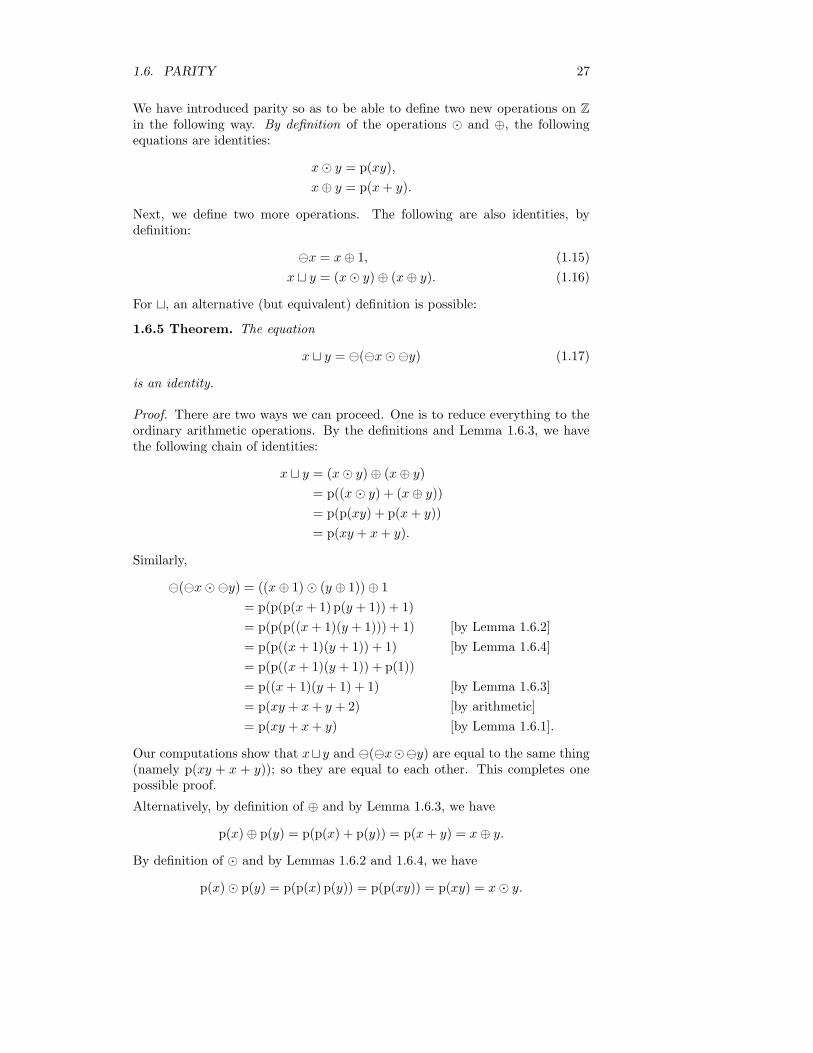
1.6. PARITY 27
We have introduced parity so as to be able to define two new operations on Zin the following way. By definition of the operations ¯ and ⊕, the followingequations are identities:
x¯ y = p(xy),
x⊕ y = p(x+ y).
Next, we define two more operations. The following are also identities, bydefinition:
ªx = x⊕ 1, (1.15)
x t y = (x¯ y)⊕ (x⊕ y). (1.16)
For t, an alternative (but equivalent) definition is possible:
1.6.5 Theorem. The equation
x t y = ª(ªx¯ªy) (1.17)
is an identity.
Proof. There are two ways we can proceed. One is to reduce everything to theordinary arithmetic operations. By the definitions and Lemma 1.6.3, we havethe following chain of identities:
x t y = (x¯ y)⊕ (x⊕ y)= p((x¯ y) + (x⊕ y))= p(p(xy) + p(x+ y))
= p(xy + x+ y).
Similarly,
ª(ªx¯ªy) = ((x⊕ 1)¯ (y ⊕ 1))⊕ 1
= p(p(p(x+ 1) p(y + 1)) + 1)
= p(p(p((x+ 1)(y + 1))) + 1) [by Lemma 1.6.2]
= p(p((x+ 1)(y + 1)) + 1) [by Lemma 1.6.4]
= p(p((x+ 1)(y + 1)) + p(1))
= p((x+ 1)(y + 1) + 1) [by Lemma 1.6.3]
= p(xy + x+ y + 2) [by arithmetic]
= p(xy + x+ y) [by Lemma 1.6.1].
Our computations show that xt y and ª(ªx¯ªy) are equal to the same thing(namely p(xy + x + y)); so they are equal to each other. This completes onepossible proof.
Alternatively, by definition of ⊕ and by Lemma 1.6.3, we have
p(x)⊕ p(y) = p(p(x) + p(y)) = p(x+ y) = x⊕ y.
By definition of ¯ and by Lemmas 1.6.2 and 1.6.4, we have
p(x)¯ p(y) = p(p(x) p(y)) = p(p(xy)) = p(xy) = x¯ y.

28 CHAPTER 1. INTRODUCTION
Therefore, to verify any identity involving only ¯ and ⊕ (and operations derivedfrom them, likeª and t), it suffices to replace each variable with its parity. Moreprecisely, to verify (1.17), it is enough to check the four possibilities when x andy are chosen from the set 0, 1. We have the following computations:
x y x¯ y x⊕ y x t y ªx ªy ªx¯ªy ª(ªx¯ªy)0 0 0 0 0 1 1 1 01 0 0 1 1 0 1 0 10 1 0 1 1 1 0 0 11 1 1 0 1 0 0 0 1
The columns headed by the two members of Equation (1.17) are identical, sothis equation is an identity.
Either of the two proofs just offered should be sufficient to establish the theoremas true. Note well the format of the first proof. The aim was to arrive atEquation (1.17). The proof did not begin with this equation; it began with oneof the members of the equation and showed that it was equal to a new term.Then the other member of Equation (1.17) was shown to be equal to the sameterm. To write the proof as follows would not be good style:
x t y ?= ª(ªx¯ªy),
(x¯ y)⊕ (x⊕ y) ?= ((x⊕ 1)¯ (y ⊕ 1))⊕ 1,
p((x¯ y) + (x⊕ y)) ?= p(p(p(x+ 1) p(y + 1)) + 1),
. . .?= . . . ,
p(xy + x+ y) = p(xy + x+ y).
(1.18)
Do not write proofs this way! What’s wrong with this style of writing? It doesnot show the connexion between consecutive lines. The Equations (1.18) don’ttell the reader, for example, that ª(ªx¯ªy) = ((x⊕ 1)¯ (y⊕ 1))⊕ 1. In fact,the equations tell us nothing that can be assumed to be correct.
Think of the following example:
−1 ?= 1
(−1)2 ?= (1)2
1 = 1.
(1.19)
It certainly does not show that −1 = 1.
If you is searching for a proof of (1.17), then you might possibly write somethinglike the Equations (1.18). Then, after you have found a correct line of argument,you should rewrite your findings before presenting them to somebody else as aproof. The next chapter will make this point again with the notion of formalproof : What one writes down when looking for a formal proof is generally a lotdifferent from the formal proof itself.

1.7. BOOLEAN CONNECTIVES 29
Exercises
(1) Prove Lemmas 1.6.2, 1.6.3 and 1.6.4.
(2) Explain why the Equations (1.19) do not constitute a valid proof of theequation −1 = 1.
(3) Suppose à is a new arithmetic operation defined on the set 0, 1 asfollows:
x y xà y0 0 11 0 10 1 01 1 1
Find an arithmetic term t such that the equation p(t) = p(x) Ã p(y) isan identity.
1.7 Boolean connectives
In memory of George Boole,42 let us refer to the set 0, 1 as B. In the lastsection, we defined some operations that convert integers into elements of B.Considering the elements of B as integers, we shall now restrict those operationson Z so as to apply only to elements of B. In so doing, we shall change theirnames:
on Z: ⊗ ⊕ ª ton B: ∧ = ¬ ∨
We shall not use the four operations ⊗, ⊕, ª and t any more. Operations onB can be called (Boolean) connectives. Specific English names can be givenas follows:
(∗) ∧ is conjunction;
(†) ¬ is negation;
(‡) ∨ is (inclusive) disjunction;
(§) = is exclusive disjunction or (material) non-equivalence.
Since B is finite, the definitions of connectives can be given in tables like thetable in the last subsection:
P Q P ∧ Q P ∨Q P = Q0 0 0 0 01 0 0 1 10 1 0 1 11 1 1 1 0
P ¬P0 11 0
It will be convenient to have two more connectives, namely:
42See for example [4, III.12, [47], p. 51].

30 CHAPTER 1. INTRODUCTION
(¶) (material) implication or the conditional: →;
(‖) (material) equivalence or the biconditional: ↔.
Again the definitions can be given in a table:
P Q P → Q P ↔ Q0 0 1 11 0 0 00 1 1 01 1 1 1
Certain identities should be evident: For example, P = Q seems to mean thesame thing as ¬(P ↔ Q). Here though, we shall not put a sign of equalitybetween the two expressions. Rather, as will be discussed more fully in § 2.2,we shall write
P = Q ∼ ¬(P ↔ Q), (1.20)
using the sign ∼ rather than the sign of equality. Why? First, by analogy withthe definition of arithmetic terms in § 1.3, we defineBoolean terms inductivelyas follows. First, Boolean terms are certain strings containing (some of) thefollowing symbols:
• ∧, ¬, ∨, =,→,↔ (or other connectives, should we choose to define them);
• the constants 0 and 1;
• variable from the list P0, P1, P2, . . . ;
• the parentheses ( and ).
Then the Boolean terms are determined by the following rules:
(∗) variables and constants are Boolean terms;
(†) if F is a Boolean term, then so is ¬F ;(‡) if F and G are Boolean terms, then so is (P ∗ Q), where ∗ is one of the
connectives ∧, ∨, =, →, ↔.
Note that the constants 0 and 1 can also be considered as Boolean connectives,since they give values (namely, themselves) in B.
We could now define Boolean polynomials and form from them what me mightcall Boolean polynomial equations; these would be examples of so-called Booleanformulas. We shall not use such expressions however, since our main interestwill lie in Boolean terms as such. To suggest this, we shall refer to Booleanterms mainly as (propositional) formulas.
As with arithmetic terms, so with propositional formulas, we can establish aconventional order of operations so as to avoid writing too many parentheses.We can always leave out an outer pair of parentheses.
• ¬ has priority over all other connectives;
• ∧ and ∨ have priority over →, ↔, and =;
• in case of two instances of →, the one on the right has priority43;
43We shall use this convention, because propositional formulas like (P0 → (P1 → P2)) aremore common than ((P0 → P1) → P2); so it will be convenient to let P0 → P1 → P2 standfor the former.

1.7. BOOLEAN CONNECTIVES 31
• in case of two instances of ∧ or of ∨ or of =, the one on the right haspriority.44
Also, instead of writing variables Pk, we may use P , Q and R instead. Similarly,we may use letters like F , G and H to stand for formulas.45
1.7.1 Examples. By the order of operations,
(∗) the Boolean term denoted by P → Q ∨R is (P → (Q ∨R));(†) ¬P ∧ Q is ((¬P ) ∧ Q);
(‡) P ∧ Q ∨R is ambiguous; the writer must say whether (P ∧ Q) ∨R orP ∧ (Q ∨R) is intended;
(§) P ∧ Q ∧ R is (P ∧ (Q ∧ R));(¶) P ∧ Q ∧ R ∨ P is ambiguous;
(‖) P → Q→ R is P → (Q→ R);
(∗∗) P = Q = R is (P = (Q = R));
(††) P → Q ∧ R→ S is (P → ((Q ∧ R)→ S)). •
A propositional formula like 0 → 1 can be called closed, because it has novariables. By definition of the connective→, this formula 0→ 1 has the value 1.The formulas 0 → 1 and 1 are not equal as formulas; but the former can beconsidered as a name for the latter (considered as an element of B).
Propositional formulas are so defined that every closed formula is the name of aunique element of B. We shall prove this in § 2.1; meanwhile, some applicationsare in the following exercises:
Exercises
(1) Which Boolean terms, if any, are denoted by the following?—
(a) P ∧ ¬Q = R ∨ P ;(b) P → Q = R;
(c) P0 → P1 → P2 → P3;
(d) P0 → P1 → · · · → Pn.
(2) The following closed formulas are names of which elements of B?—
(a) 1→ 1→ 1,
(b) 1→ 0→ 1,
(c) (0→ 1)↔ 1,
(d) ¬(0 = 1)↔ (0↔ 1),
(e) ¬¬¬0,(f) (1 ∨ 0) ∧ 0,
(g) (1 ∨ (0 ∧ 0).
44We could just as well give priority to the one on the left; we just want to allow ourselvesto let strings like P ∧ Q ∧ R denote Boolean terms.
45The symbols P0, P1 and so on are the variables that can appear officially in Booleanterms. The symbols P , Q and so on are variables that we use to talk about Boolean terms:they are syntactical variables in the sense of [7, § 08]. Likewise, F and so on are not literallyformulas; we use them as syntactical variables for formulas.
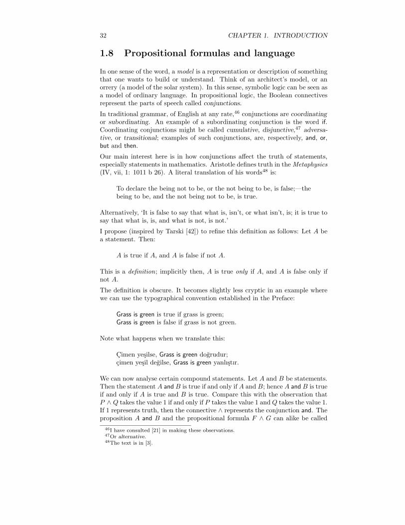
32 CHAPTER 1. INTRODUCTION
1.8 Propositional formulas and language
In one sense of the word, a model is a representation or description of somethingthat one wants to build or understand. Think of an architect’s model, or anorrery (a model of the solar system). In this sense, symbolic logic can be seen asa model of ordinary language. In propositional logic, the Boolean connectivesrepresent the parts of speech called conjunctions.
In traditional grammar, of English at any rate,46 conjunctions are coordinatingor subordinating. An example of a subordinating conjunction is the word if.Coordinating conjunctions might be called cumulative, disjunctive,47 adversa-tive, or transitional; examples of such conjunctions, are, respectively, and, or,but and then.
Our main interest here is in how conjunctions affect the truth of statements,especially statements in mathematics. Aristotle defines truth in theMetaphysics(IV, vii, 1: 1011 b 26). A literal translation of his words48 is:
To declare the being not to be, or the not being to be, is false;—thebeing to be, and the not being not to be, is true.
Alternatively, ‘It is false to say that what is, isn’t, or what isn’t, is; it is true tosay that what is, is, and what is not, is not.’
I propose (inspired by Tarski [42]) to refine this definition as follows: Let A bea statement. Then:
A is true if A, and A is false if not A.
This is a definition; implicitly then, A is true only if A, and A is false only ifnot A.
The definition is obscure. It becomes slightly less cryptic in an example wherewe can use the typographical convention established in the Preface:
Grass is green is true if grass is green;Grass is green is false if grass is not green.
Note what happens when we translate this:
Cimen yesilse, Grass is green dogrudur;cimen yesil degilse, Grass is green yanlıstır.
We can now analyse certain compound statements. Let A and B be statements.Then the statement A and B is true if and only if A and B; hence A and B is trueif and only if A is true and B is true. Compare this with the observation thatP ∧ Q takes the value 1 if and only if P takes the value 1 and Q takes the value 1.If 1 represents truth, then the connective ∧ represents the conjunction and. Theproposition A and B and the propositional formula F ∧ G can alike be called
46I have consulted [21] in making these observations.47Or alternative.48The text is in [3].

1.8. PROPOSITIONAL FORMULAS AND LANGUAGE 33
conjunctions. Note well, however, that the proposition A and B belongs toour ordinary language, while the formula F ∧ G belongs to propositional logic.
Similarly, A or B is true if and only if A is true or B is true. Also, P ∨Q takesthe value 1 if and only if P takes the value 1, or Q takes the value 1. So theconnective ∨ represents the conjunction or. The proposition A or B and thepropositional formula F ∨G can alike be called disjunctions.
More precisely, ∨ represents or in its inclusive sense. The exclusive sense of oris intended in a sentence like You may have tea or coffee after your meal, if thismeans that you are allowed to have tea, and you are allowed to have coffee,but you are not allowed to have both. The exclusive or is represented by theconnective =.
The sentence Not-A is true if and only if A is false; and ¬P takes the value 1if and only if P takes the value 0. If now 0 represents falsity, then ¬ representsnot. Both Not-A and ¬F can be called negations. (In fact the negation of anEnglish statement is almost never formed simply by the prefixing of the wordnot; the not goes inside, perhaps with some other changes.)
Mathematics often involves ignoring certain distinctions. From the propositionsA and B, we can form several compound propositions:
A and BA, but BA; B
Each of these may have its own rhetorical coloration, but we shall take them allto have the same truth-value. We may use for any of them the abbreviation
A & B.
One could write also A ∧ B; but I prefer to reserve ∧ for use in propositionalformulas as defined in the previous section. The sentence A & B here is not apropositional formula; it is just a proposition or sentence of ordinary language.
We can form some more compounds:
If A, then BWhen A, then BA implies BB if A
A only if B
These can be called implications and conditional statements. Each of themhas the antecedent A and the consequent B. We shall understand the com-pounds to be true if B is true or A is false (or both); otherwise, the compoundsare false. We may use the abbreviation
A =⇒ B
The propositional formula P → Q can be analysed similarly, and we can applythe same terminology.

34 CHAPTER 1. INTRODUCTION
In ordinary language, the sentence If A, then B suggests causation. If you dropthat Iznik vase, then it will break—you will cause the vase to break by droppingit. In mathematics though, If A, then B means no more than B is true or A isfalse. This is why we referred to → as material implication49: Here materialis opposed to formal. The idea is that, in the sentence about a vase, there is a‘formal’ connexion between antecedent and consequent: they both refer to thesame vase, for example. Such a connexion is missing in a sentence like If wateris wet, then Constantine founded Constantinople; but we count the sentence as‘materially’ true if we accept the consequent as true. (In this case, it is irrelevantthat the antecedent is true.)
There is a saying in English, If wishes were horses, then beggars would ride. Wecan’t analyse this as a material implication, simply because the antecedent andconsequent are not propositions. We can try to recast the sentence as, If wishesare horses, then beggars ride. Then we can argue that the sentence is true, simplybecause the antecedent is false: wishes are not horses. This observation saysnothing about the truth of the original saying.
In some mathematical writing, one sees statements like
A =⇒ B =⇒ C.
This should be understood as an abbreviation for
(A =⇒ B) & (B =⇒ C).
This conjunction is not the same statement as the implication
A =⇒ (B =⇒ C),
even though we understand the formula F → G→ H as an abbreviation for theformula F → (G→ H).
In ordinary language, we can write indifferently
A if and only if BA just in case B
These are equivalences and biconditional statements, and for them we canuse the abbreviation
A ⇐⇒ B.
The formula P ↔ Q has a similar analysis and description.
Some fundamental rules of reasoning can be abbreviated thus:
A & (A =⇒ B) =⇒ B; (1.21)
not-(A =⇒ B) ⇐⇒ A & not-B. (1.22)
(We are using a convention like that established in § 1.7: the & has priorityover =⇒ and ⇐⇒ .)
The operations of conversion and contraposition can be performed on im-plications:
49See the discussions in [7, § 05, n. 89, pp. 37f.] or [43, §§ 8, 9].

1.9. QUANTIFIERS 35
(∗) The converse of A =⇒ B is B =⇒ A;
(†) the contrapositive of A =⇒ B is not-B =⇒ not-A.
The contrapositive of an implication is true if and only if the original implicationis true:
(A =⇒ B) ⇐⇒ (not-B =⇒ not-A).
This observation is of great value in the proving of mathematical propositions.
Exercises
(1) Find a true implication whose converse is true.
(2) Find a true implication whose converse is false.
1.9 Quantifiers
As the Boolean connectives are used to model the conjunctions of ordinary lan-guage, so the symbols called quantifiers can be used to model certain adjectives,especially all and some. Quantifiers are a part of predicate logic. To see howgood this logic is as a model of ordinary language, I propose first to look atordinary adjectives in general, as they are used in English.
I here understand an adjective to be a word or phrase found in association witha noun—a noun that the adjective is said to modify. For example, I understandthe definite article, the, and the indefinite article, a/an, to be adjectives.While the can be used with singular and plural nouns, a is used only withsingular nouns. The articles are of use in establishing a fourfold classificationof adjectives:
(∗) Most adjectives in the dictionary are descriptive, like green, good, better,first, second, . . . , single, double, . . . , contradictory and numerous. Any ofthese can be preceded by an article: the green grass; a second opinion.A descriptive adjective describes—names a property or quality of—theobject or objects named by the associated noun: Green grass is grasswith the property of being green. The property named by a descriptiveadjective may fail to belong strictly to the object or objects named bythe associated noun; it may belong to the relation of these objects withothers: A second opinion can be second only if there is also a first opinion.
(†) The demonstrative adjectives include this/these, that/those, which, theand the same. Note that this/these and that/those are peculiar, as adjec-tives, for having distinct singular and plural forms. The demonstrativeadjectives indicate that a certain, a particular, a definite object is namedby the associated noun. They cannot be preceded by an article: We cannotrefer to the this tree or a the mountain.
(‡) The quantitative adjectives include zero, one, two, . . . , few, several, many,little, much. The name quantitative seems appropriate for these adjectives,although they will not be symbolized by the so-called quantifiers. Someof the quantitative adjectives are symbolized by the numerals 0, 1, 2, . . .A quantitative adjective can be preceded by the definite article, but not

36 CHAPTER 1. INTRODUCTION
dual manifold
negative sing. neither nopl. no
existential sing. either a/an, any, somepl. some, a few, a little, a great many
universal sing. either a/an, any, each, everypl. both all
Figure 1.2: Logical adjectives. The labels sing. and pl. indicate whether anadjective on that line is associated with a singular or a plural noun. The labelsdual and manifold indicate whether the noun associated with an adjective in thatcolumn names an element (or elements) of a set of size two or more than two.
by the indefinite article: We can refer to the two opinions, but not to aone opinion. We can mention a few opinions; but I put a few in the finalclass:
(§) The logical adjectives are the remaining: neither, no, either, a/an, any,some, both, a few, a little, a great many, each, every, all. They cannot bepreceded by an article.
Some grammarians50 refer to the demonstrative, quantitative and logical ad-jectives as determiners. Determiners are distinguished from other adjectives bybeing more fundamental parts of language—and by never being preceded by theindefinite article.
The logical adjectives can be arranged as in Figure 1.2. The main point to noteis that there are three kinds of logical adjectives, which I am calling negative,existential and universal.
In a section of the ‘XVII. Meditation’ of his Devotions upon Emergent Occasionsof 1624, the clergyman and metaphysical poet John Donne uses three logicaladjectives in addition to the indefinite article. The Meditation begins as follows(and here I preserve Donne’s original spelling and typography, as found in [11,pp. 440f.]): ‘Perchance hee for whom this Bell tolls, may be so ill, as that heknowes not it tolls for him;’ later, the Meditation continues:
No man is an Iland, intire of it selfe; every man is a peece of theContinent, a part of the maine; if a Clod bee washed away by theSea, Europe is the lesse, as well as if a Promontorie were, as well asif a Mannor of thy friends or of thine owne were; any mans deathdiminishes me, because I am involved in Mankinde; And thereforenever send to know for whom the bell tolls; It tolls for thee.
Note the three clauses (and now I modernize the spelling):
No man is an island.Every man is a piece of the continent.Any man’s death diminishes me.
50For example, the editor of the ninth edition of the Concise Oxford Dictionary [46]; however,she treats one and two, like first, as ordinary [descriptive] adjectives.
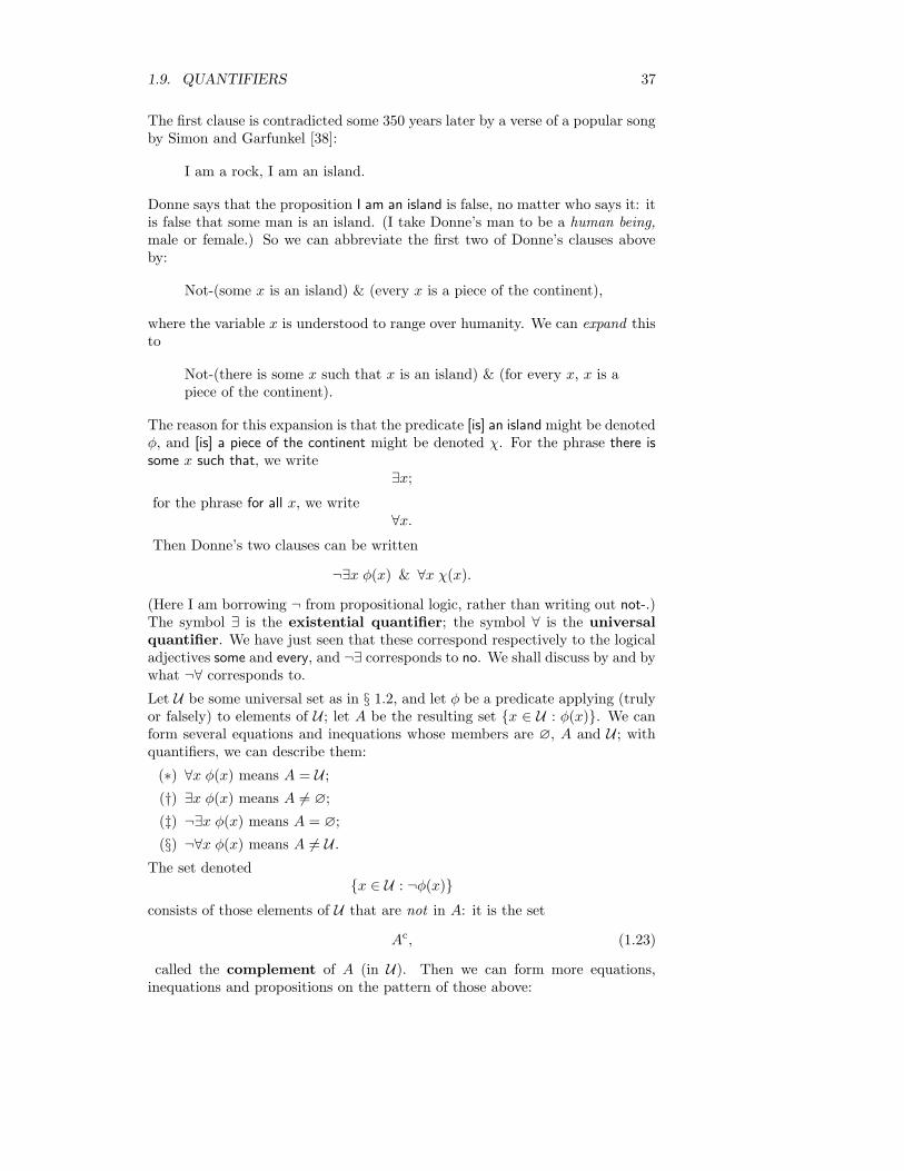
1.9. QUANTIFIERS 37
The first clause is contradicted some 350 years later by a verse of a popular songby Simon and Garfunkel [38]:
I am a rock, I am an island.
Donne says that the proposition I am an island is false, no matter who says it: itis false that some man is an island. (I take Donne’s man to be a human being,male or female.) So we can abbreviate the first two of Donne’s clauses aboveby:
Not-(some x is an island) & (every x is a piece of the continent),
where the variable x is understood to range over humanity. We can expand thisto
Not-(there is some x such that x is an island) & (for every x, x is apiece of the continent).
The reason for this expansion is that the predicate [is] an islandmight be denotedφ, and [is] a piece of the continent might be denoted χ. For the phrase there issome x such that, we write
∃x;for the phrase for all x, we write
∀x.Then Donne’s two clauses can be written
¬∃x φ(x) & ∀x χ(x).
(Here I am borrowing ¬ from propositional logic, rather than writing out not-.)The symbol ∃ is the existential quantifier; the symbol ∀ is the universalquantifier. We have just seen that these correspond respectively to the logicaladjectives some and every, and ¬∃ corresponds to no. We shall discuss by and bywhat ¬∀ corresponds to.
Let U be some universal set as in § 1.2, and let φ be a predicate applying (trulyor falsely) to elements of U ; let A be the resulting set x ∈ U : φ(x). We canform several equations and inequations whose members are ∅, A and U ; withquantifiers, we can describe them:
(∗) ∀x φ(x) means A = U ;(†) ∃x φ(x) means A 6= ∅;
(‡) ¬∃x φ(x) means A = ∅;
(§) ¬∀x φ(x) means A 6= U .The set denoted
x ∈ U : ¬φ(x)consists of those elements of U that are not in A: it is the set
Ac, (1.23)
called the complement of A (in U). Then we can form more equations,inequations and propositions on the pattern of those above:
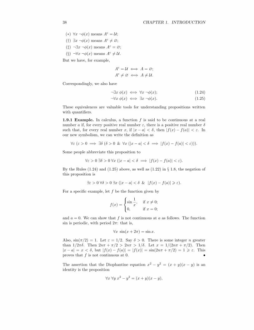
38 CHAPTER 1. INTRODUCTION
(∗) ∀x ¬φ(x) means Ac = U ;(†) ∃x ¬φ(x) means Ac 6= ∅;
(‡) ¬∃x ¬φ(x) means Ac = ∅;
(§) ¬∀x ¬φ(x) means Ac 6= U .But we have, for example,
Ac = U ⇐⇒ A = ∅;
Ac 6= ∅ ⇐⇒ A 6= U .
Correspondingly, we also have
¬∃x φ(x) ⇐⇒ ∀x ¬φ(x); (1.24)
¬∀x φ(x) ⇐⇒ ∃x ¬φ(x). (1.25)
These equivalences are valuable tools for understanding propositions writtenwith quantifiers.
1.9.1 Example. In calculus, a function f is said to be continuous at a realnumber a if, for every positive real number ε, there is a positive real number δsuch that, for every real number x, if |x− a| < δ, then |f(x)− f(a)| < ε. Inour new symbolism, we can write the definition as
∀ε (ε > 0 =⇒ ∃δ (δ > 0 & ∀x (|x− a| < δ =⇒ |f(x)− f(a)| < ε))).
Some people abbreviate this proposition to
∀ε > 0 ∃δ > 0 ∀x (|x− a| < δ =⇒ |f(x)− f(a)| < ε).
By the Rules (1.24) and (1.25) above, as well as (1.22) in § 1.8, the negation ofthis proposition is
∃ε > 0 ∀δ > 0 ∃x (|x− a| < δ & |f(x)− f(a)| > ε).
For a specific example, let f be the function given by
f(x) =
sin
1
x, if x 6= 0;
0, if x = 0;
and a = 0. We can show that f is not continuous at a as follows. The functionsin is periodic, with period 2π: that is,
∀x sin(x+ 2π) = sinx.
Also, sin(π/2) = 1. Let ε = 1/2. Say δ > 0. There is some integer n greaterthan 1/2πδ. Then 2nπ + π/2 > 2nπ > 1/δ. Let x = 1/(2nπ + π/2). Then|x− a| = x < δ, but |f(x)− f(a)| = |f(x)| = sin(2nπ + π/2) = 1 > ε. Thisproves that f is not continuous at 0. •
The assertion that the Diophantine equation x2 − y2 = (x + y)(x − y) is anidentity is the proposition
∀x ∀y x2 − y2 = (x+ y)(x− y),
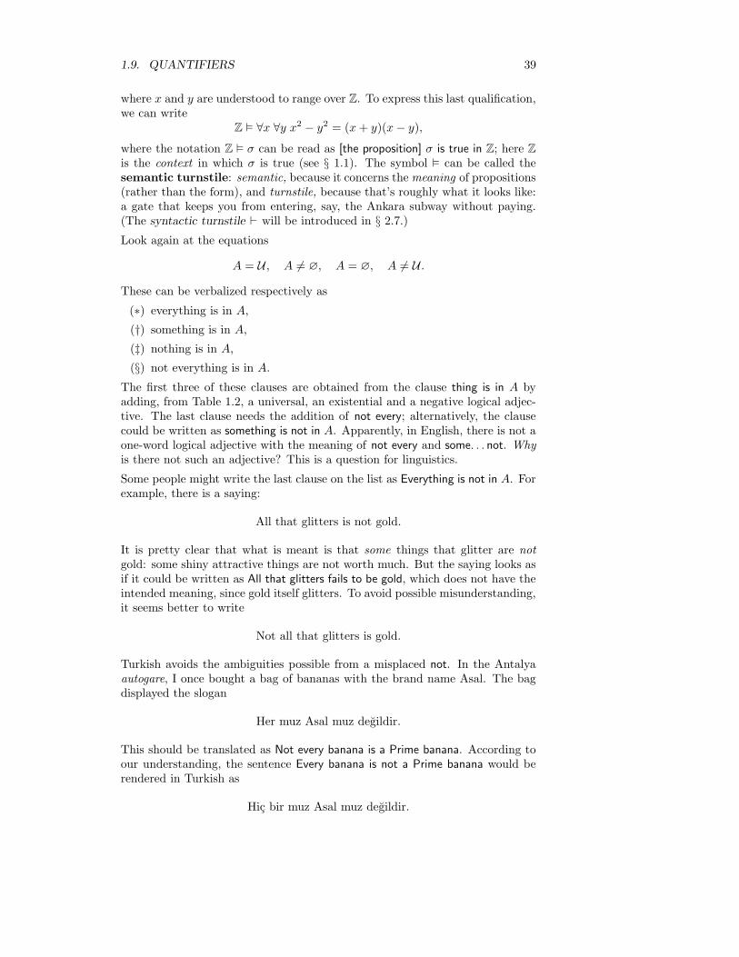
1.9. QUANTIFIERS 39
where x and y are understood to range over Z. To express this last qualification,we can write
Z ² ∀x ∀y x2 − y2 = (x+ y)(x− y),where the notation Z ² σ can be read as [the proposition] σ is true in Z; here Zis the context in which σ is true (see § 1.1). The symbol ² can be called thesemantic turnstile: semantic, because it concerns themeaning of propositions(rather than the form), and turnstile, because that’s roughly what it looks like:a gate that keeps you from entering, say, the Ankara subway without paying.(The syntactic turnstile ` will be introduced in § 2.7.)Look again at the equations
A = U , A 6= ∅, A = ∅, A 6= U .
These can be verbalized respectively as
(∗) everything is in A,
(†) something is in A,
(‡) nothing is in A,
(§) not everything is in A.
The first three of these clauses are obtained from the clause thing is in A byadding, from Table 1.2, a universal, an existential and a negative logical adjec-tive. The last clause needs the addition of not every; alternatively, the clausecould be written as something is not in A. Apparently, in English, there is not aone-word logical adjective with the meaning of not every and some. . . not. Whyis there not such an adjective? This is a question for linguistics.
Some people might write the last clause on the list as Everything is not in A. Forexample, there is a saying:
All that glitters is not gold.
It is pretty clear that what is meant is that some things that glitter are notgold: some shiny attractive things are not worth much. But the saying looks asif it could be written as All that glitters fails to be gold, which does not have theintended meaning, since gold itself glitters. To avoid possible misunderstanding,it seems better to write
Not all that glitters is gold.
Turkish avoids the ambiguities possible from a misplaced not. In the Antalyaautogare, I once bought a bag of bananas with the brand name Asal. The bagdisplayed the slogan
Her muz Asal muz degildir.
This should be translated as Not every banana is a Prime banana. According toour understanding, the sentence Every banana is not a Prime banana would berendered in Turkish as
Hic bir muz Asal muz degildir.
40 CHAPTER 1. INTRODUCTION
Should we have symbols for the other adjectives in Table 1.2, besides no, someand all? Probably not. The sentence Neither x is in A means A = ∅, providedthat x ranges over a universe with just two elements (and A is a subset of thisuniverse). The distinction between a pair and a multitude is perhaps importantin a life where many things come in pairs (like married couples, teams of oxen,and eyeballs); but we need not make the distinction logically, with fundamentalsymbols, if we are just trying to do mathematics.
The word either is ambiguous: If I tell you that you may have either piece ofcake, does this mean you can have both? Maybe, maybe not. Likewise, a/anand any are ambiguous. If you say A dog has three legs, you probably meanthe a existentially: there is a dog that has three legs. But if you say A dog hasfour legs, probably you are describing dogs in general: every dog has four legs.The sentence Anybody can come could be a general invitation to everybody, orit could express a worry over the possibility that somebody will come.
Still, the word any seems useful in ordinary life. Again, Donne writes:
Any man’s death diminishes me.
Could he write, instead, Every man’s death diminishes me? In a mathematicalcontext, the every is preferable; but every man’s death suggests the image ofall people dying at once; any man’s death takes the deaths one by one. It’s adistinction that matters to a poet.
Exercises
(1) Write a sentence equivalent to ∀x ∃y ψ(x, y) that does not use ∃.
(2) Discuss the logical adjectives of Turkish (or some other language besidesEnglish).

Chapter 2
Propositional logic
2.0 Truth-tables
We have defined propositional formulas in § 1.7. For every closed propositionalformula F , there is an element
F
of B that can be found in the following way. First note that F meets one of thefollowing conditions:
(∗) F is a constant from B (that is, 0 or 1), or
(†) F is ¬G for some closed formula G, or
(‡) F is (G ∗ H) for some closed formulas G and H, where ∗ is one of theconnectives ∧, ∨, →, ↔ and =.
Then we can find F by the following recursive procedure:
(∗) If F is in B, then F is F itself;
(†) if F is ¬G, then F is the value of ¬G as determined by the table in § 1.7;(‡) if F is (G ∗H), then F is the value of G ∗ H as determined by the tables
in § 1.7.In the terminology introduced at the end of § 1.7, F is a name for F . It isproved in the next next section below that F is uniquely determined by theprocedure for finding it; we can then call F the (truth)-value of F .
If a formula is not closed, then it doesn’t have a value in B. But any formulacan be made into a closed formula by substitution of values for its variables.
If the variables in a propositional formula F belong to the set P0, P1, . . . , Pn−1,then we can indicate this by writing F as F (P0, . . . , Pn−1); we may also call Fan n-ary formula.1 A 3-ary formula would be ternary; 2-ary, binary; 1-ary,singulary.2 A 0-ary or nullary formula would have no variables: it would be
1Here F is a syntactical variable as discussed in Chapter 1, n. 45.2The word unary is often used instead of singulary. Following Quine, Church [7, § 02,
p. 12, n. 29] suggests singulary as a more etymologically correct word than unary. Indeed,whereas the first five Latin cardinal numbers are un-, du-, tri-, quattuor, quinque, the
41

42 CHAPTER 2. PROPOSITIONAL LOGIC
closed in the sense of § 1.7. An n-ary formula is also (n + 1)-ary, (n + 2)-ary,and so on.
2.0.1 Examples.
(1) Suppose F is P0 ∧ P1 → P0 ∨ P1 (that is, ((P0 ∧ P1) → (P0 ∨ P1)),according to the convention established in § 1.7). Then F is binary andcan be described as
F (P0, P1).
It can also be considered as the ternary formula F (P0, P1, P2), but not asthe singulary F (P0).
(2) By the convention established here, the formula P4 ∨P21 is 22-ary and175-ary; it is not 21-ary, much less binary. •
If F is an (n + 1)-ary formula, then it can be converted to an n-ary formulain two different ways by substitution. Indeed, if e is one of the two elementsof B, then each occurrence of the variable Pn in F can be replaced with e; allthe remaining variables of F belong to P0, . . . , Pn−1, so F has become n-ary.In turn, other elements of B can be substituted for other variables in F , so asto obtain, in the end, a closed formula.
In general, if F is an n-ary formula, and (e0, . . . , en−1) is a list of n elementsof B, then there is a closed formula
F (e0, . . . , en−1),
which is the result of subtituting ek for Pk in F for each k less than n. The list(e0, . . . , en−1) can be called an n-tuple from B and can be abbreviated as
e or ~e .
(The definition of n-tuple will be refined in § 3.2.) Here the tuple ~e is an n-arytruth-assignment (or a truth-assignment for F ). The truth-value of F (~e )can be denoted3
F (~e ).
2.0.2 Example. Again suppose F is P0 ∧ P1 → P0 ∨ P1; consider this asF (P0, P1). If ~e = (0, 1), then F (~e ) is 0 ∧ 1 → 0 ∨ 1; the value of this is the
value of 0→ 1, which is 1. That is, F (0, 1) = 1. •
A truth-table is a list of the values attained by a propositional formula underits possible truth-assignments. If a formula is n-ary, then its truth-table hasn + 1 columns: a column for each variable, and one column for the formulaitself; also, aside from the headings of the columns, the table must have 2n
rows.
first five Latin distributive numbers—corresponding to the Turkish birer, ikiser, ucer, dorder,beser [30]—are singul-, bin-, tern-, quatern-, quin-. It is the latter sequence that gives usbinary and ternary—also quaternary and quinary, if these are desired. So singulary appears tobe a better word than unary. In fact, singulary does not appear in the original Oxford English
Dictionary [28]. The word unary does appear in this dictionary, but it is considered obsolete:only one use of the word, from 1576, was discovered in English literature. There, unary meantunit, although the word unit was not actually invented until 1570, when it was introduced by[John] Dee to correspond to the Greek monad-.
3The notation is from [5, Definition 2.1.8, p. 41].
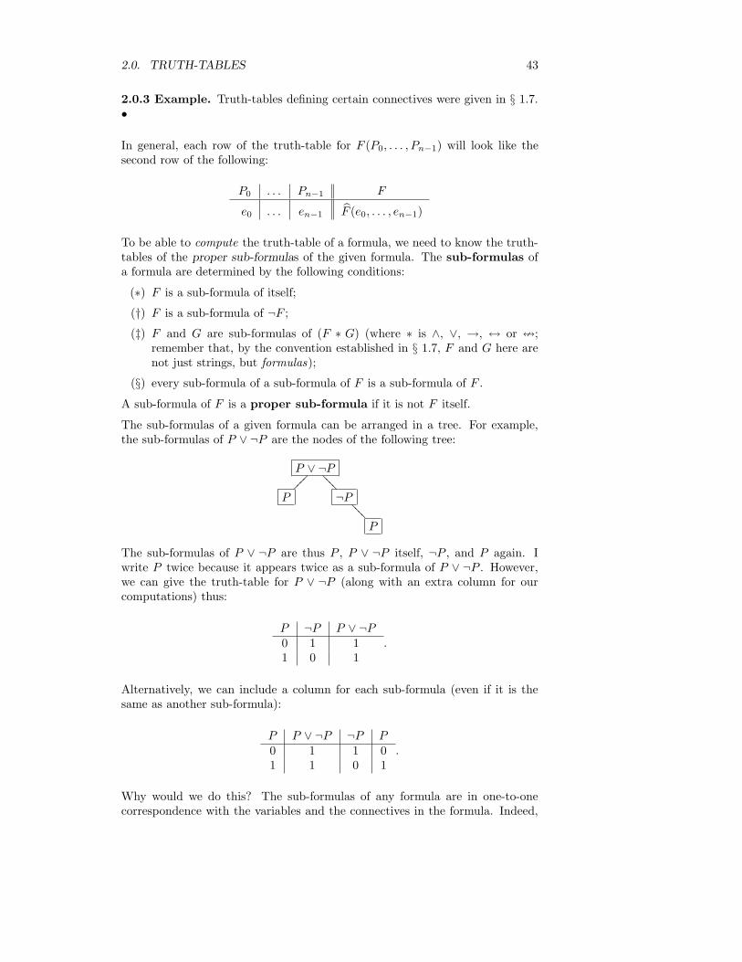
2.0. TRUTH-TABLES 43
2.0.3 Example. Truth-tables defining certain connectives were given in § 1.7.•
In general, each row of the truth-table for F (P0, . . . , Pn−1) will look like thesecond row of the following:
P0 . . . Pn−1 F
e0 . . . en−1 F (e0, . . . , en−1)
To be able to compute the truth-table of a formula, we need to know the truth-tables of the proper sub-formulas of the given formula. The sub-formulas ofa formula are determined by the following conditions:
(∗) F is a sub-formula of itself;
(†) F is a sub-formula of ¬F ;(‡) F and G are sub-formulas of (F ∗ G) (where ∗ is ∧, ∨, →, ↔ or =;
remember that, by the convention established in § 1.7, F and G here arenot just strings, but formulas);
(§) every sub-formula of a sub-formula of F is a sub-formula of F .
A sub-formula of F is a proper sub-formula if it is not F itself.
The sub-formulas of a given formula can be arranged in a tree. For example,the sub-formulas of P ∨ ¬P are the nodes of the following tree:
P ∨ ¬PÄÄÄÄ ??
??
P ¬P??
??
P
The sub-formulas of P ∨ ¬P are thus P , P ∨ ¬P itself, ¬P , and P again. Iwrite P twice because it appears twice as a sub-formula of P ∨ ¬P . However,we can give the truth-table for P ∨ ¬P (along with an extra column for ourcomputations) thus:
P ¬P P ∨ ¬P0 1 11 0 1
.
Alternatively, we can include a column for each sub-formula (even if it is thesame as another sub-formula):
P P ∨ ¬P ¬P P0 1 1 01 1 0 1
.
Why would we do this? The sub-formulas of any formula are in one-to-onecorrespondence with the variables and the connectives in the formula. Indeed,

44 CHAPTER 2. PROPOSITIONAL LOGIC
compare the previous tree with the following:
∨ÄÄÄÄ ??
??
P ¬??
??
P
We have the following correspondence between sub-formulas and symbols:
P ! PP ∨ ¬P ! ∨
¬P ! ¬P ! P
Using this correspondence, we can rewrite the last truth-table thus:
P ∨ ¬ P0 1 1 01 1 0 1
I propose to call this the full truth-table of P ∨ ¬P ; from it we can extractthe proper truth-table of P ∨ ¬P by taking only one column headed by P ,along and the column headed by ∨ (which corresponds to the whole formula):
P P ∨ ¬P0 11 1
For another example, let F be the formula P → ¬Q∨R. The sub-formulas of Fcompose the tree
P → ¬Q ∨RÄÄÄ
TTTTTTT
P ¬Q ∨Rooo
ooo ???
¬Q??
? R
Q
The corresponding tree of variables and connectives is:
→ÄÄÄÄ
TTTTTTTT
TTTTT
P ∨ooo
ooooo
????
¬??
?? R
Q
From this we can get the full truth-table as described below. The table itself is:
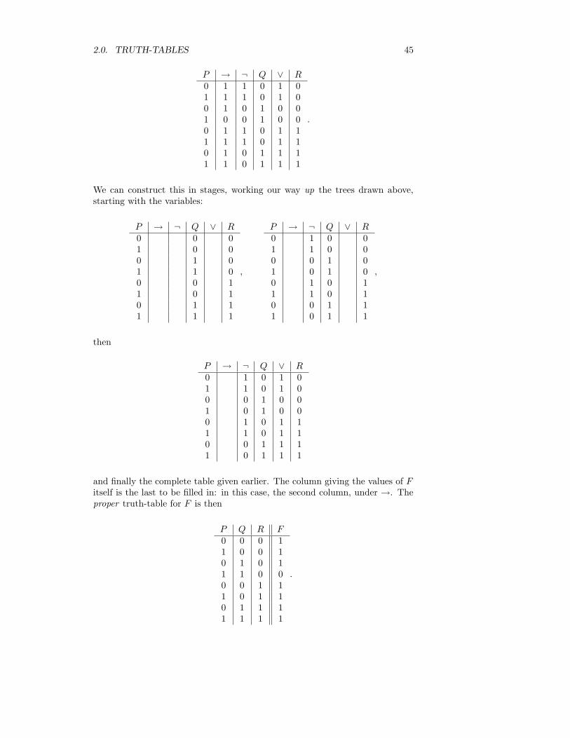
2.0. TRUTH-TABLES 45
P → ¬ Q ∨ R0 1 1 0 1 01 1 1 0 1 00 1 0 1 0 01 0 0 1 0 00 1 1 0 1 11 1 1 0 1 10 1 0 1 1 11 1 0 1 1 1
.
We can construct this in stages, working our way up the trees drawn above,starting with the variables:
P → ¬ Q ∨ R0 0 01 0 00 1 01 1 00 0 11 0 10 1 11 1 1
,
P → ¬ Q ∨ R0 1 0 01 1 0 00 0 1 01 0 1 00 1 0 11 1 0 10 0 1 11 0 1 1
,
then
P → ¬ Q ∨ R0 1 0 1 01 1 0 1 00 0 1 0 01 0 1 0 00 1 0 1 11 1 0 1 10 0 1 1 11 0 1 1 1
and finally the complete table given earlier. The column giving the values of Fitself is the last to be filled in: in this case, the second column, under →. Theproper truth-table for F is then
P Q R F0 0 0 11 0 0 10 1 0 11 1 0 00 0 1 11 0 1 10 1 1 11 1 1 1
.
46 CHAPTER 2. PROPOSITIONAL LOGIC
Exercises
(1) Write full truth-tables and proper truth-tables for the formulas:
(a) P → (Q→ P );
(b) P ∧ Q ∧ R;(c) P = Q = R;
(d) (P → Q ∨R)→ (¬P ∨Q);
(e) (P → Q ∨ ¬R) ∧ (Q→ P ∧ R)→ (P → R);
(f) ¬(¬R→ P → ¬(R→ Q)).
How many columns has each table?
(2) What does the truth-table for a constant formula look like?
(3) For each n in N, describe the n-ary formulas whose full truth-tables havefewer columns than their proper truth-tables.
2.1 Unique readability
We have to justify our definition of F for closed formulas F : that is, we have toconfirm that only one value can be computed for each F .
We have called a propositional formula n-ary if its variables are among the first nvariables on the list (P0, P1, P2, . . . ). The notion of arity applies to connectivesthemselves:
(∗) ∧, ∨,→,↔ and = are binary, because they are used to join two formulas;
(†) ¬ is singulary;
(‡) the constants 0 and 1 are nullary.
Although, by our convention, an n-ary formula is also (n+ 1)-ary, a connectivehas a unique arity: since ¬ is singulary, it is not binary.
The formulas joined by a connective in a formula are the arguments of theconnective. In the formula
P → ¬Q ∧ 1
(which stands for (P → (¬Q ∧ 1))), the arguments of → are P and ¬Q ∧ 1 (inthat order); the arguments of ∧ are ¬Q and 1; the argument of ¬ is Q; and 1has no argument.
By definition, each propositional formula F meets one of the following condi-tions:
(∗) F is a variable;
(†) F is a nullary connective;
(‡) F is ¬G for some G;
(§) F is (G ∗H) for some G and H and some binary connective ∗.
2.1. UNIQUE READABILITY 47
It is obvious that F can meet only one of these conditions. It is not obviousthat a formula (G ∗H) cannot also be written (G′ ∗′H ′), where G′ is a differentformula from G.
Let G be (P ∧ Q), and let H be R. Then (G ∨H) can be written as (S ∧ T ),where S is (P , and T is Q) ∨ R. But S is not a formula (why not?); neither isT .
How do we know that, if G and H are more complicated, (G ∗H) still cannotbe analyzed as a different application of a binary connective? How do we knowthat (G ∗ H) is uniquely readable? Our definition of F (~e ) requires uniquereadability. To prove unique readability; we can use the notion of an initialsegment of a formula.
Every formula is a string of symbols, written left to right. If we cut the string,then it is divided into two segments: an initial and a final segment. We allowthe cut to come at an end: that is, we allow one of the two segments to beempty, so that the other segment is the whole string:
2.1.1 Example. The initial segments of (P ∨¬P ) are (P ∨¬P ) itself, (P ∨¬P ,(P ∨ ¬, (P ∨ , (P , (, and the empty string. •
An initial segment of F that is not F itself is a proper initial segment of F .
2.1.2 Lemma.
(∗) Every propositional formula has just as many left parentheses as rightparentheses.
(†) If F is a variable, a constant, or a negation, then every initial segmentof F has at least as many left parentheses as right parentheses.
(‡) If F is a propositional formula that is not a variable, a constant, or anegation, then every non-empty proper initial segment of F has more leftparentheses than right parentheses.
Proof. To prove the first claim, follow the pattern of Proposition 1.2.
To prove the second and third claims, let A be the set of formulas F that dosatisfy those claims. Then, trivially, A contains all variables and constants. IfA contains F , then F has at least as many left as right parentheses, hence sodoes ¬F , which means ¬F is in A. Finally, suppose A contains F and G, and∗ is a binary connective. Every non-empty proper initial segment of (F ∗G) iseither (F ∗ S for some initial segment S of G, or (T for some initial segment Tof F . But then S and T must have at least as many left as right parentheses,since F and G are in A; so (F ∗S and (T have more left than right parentheses.Therefore (F ∗G) is in A. By the inductive definition of propositional formulas,A contains all of them.
2.1.3 Lemma. No proper initial segment of a propositional formula is a propo-sitional formula.
Proof. Let A comprise all formulas F such that no proper initial segment of Fis a formula. Then A contains all variables and constants. Suppose A containsF , and S is an initial segment of ¬F that is a formula. Then S is ¬T for some
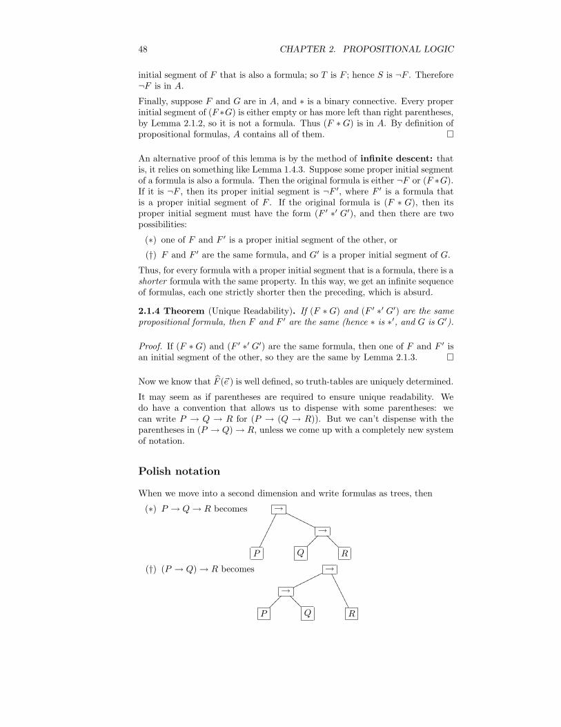
48 CHAPTER 2. PROPOSITIONAL LOGIC
initial segment of F that is also a formula; so T is F ; hence S is ¬F . Therefore¬F is in A.
Finally, suppose F and G are in A, and ∗ is a binary connective. Every properinitial segment of (F ∗G) is either empty or has more left than right parentheses,by Lemma 2.1.2, so it is not a formula. Thus (F ∗G) is in A. By definition ofpropositional formulas, A contains all of them.
An alternative proof of this lemma is by the method of infinite descent: thatis, it relies on something like Lemma 1.4.3. Suppose some proper initial segmentof a formula is also a formula. Then the original formula is either ¬F or (F ∗G).If it is ¬F , then its proper initial segment is ¬F ′, where F ′ is a formula thatis a proper initial segment of F . If the original formula is (F ∗ G), then itsproper initial segment must have the form (F ′ ∗′ G′), and then there are twopossibilities:
(∗) one of F and F ′ is a proper initial segment of the other, or
(†) F and F ′ are the same formula, and G′ is a proper initial segment of G.
Thus, for every formula with a proper initial segment that is a formula, there is ashorter formula with the same property. In this way, we get an infinite sequenceof formulas, each one strictly shorter then the preceding, which is absurd.
2.1.4 Theorem (Unique Readability). If (F ∗G) and (F ′ ∗′ G′) are the samepropositional formula, then F and F ′ are the same (hence ∗ is ∗′, and G is G′).
Proof. If (F ∗G) and (F ′ ∗′ G′) are the same formula, then one of F and F ′ isan initial segment of the other, so they are the same by Lemma 2.1.3.
Now we know that F (~e ) is well defined, so truth-tables are uniquely determined.
It may seem as if parentheses are required to ensure unique readability. Wedo have a convention that allows us to dispense with some parentheses: wecan write P → Q → R for (P → (Q → R)). But we can’t dispense with theparentheses in (P → Q)→ R, unless we come up with a completely new systemof notation.
Polish notation
When we move into a second dimension and write formulas as trees, then
(∗) P → Q→ R becomes →
²²²²²²²²²
OOOOOO
OO
→ÄÄÄÄ ??
??
P Q R
(†) (P → Q)→ R becomes →ooo
ooooo
/////////
→ÄÄÄÄ ??
??
P Q R
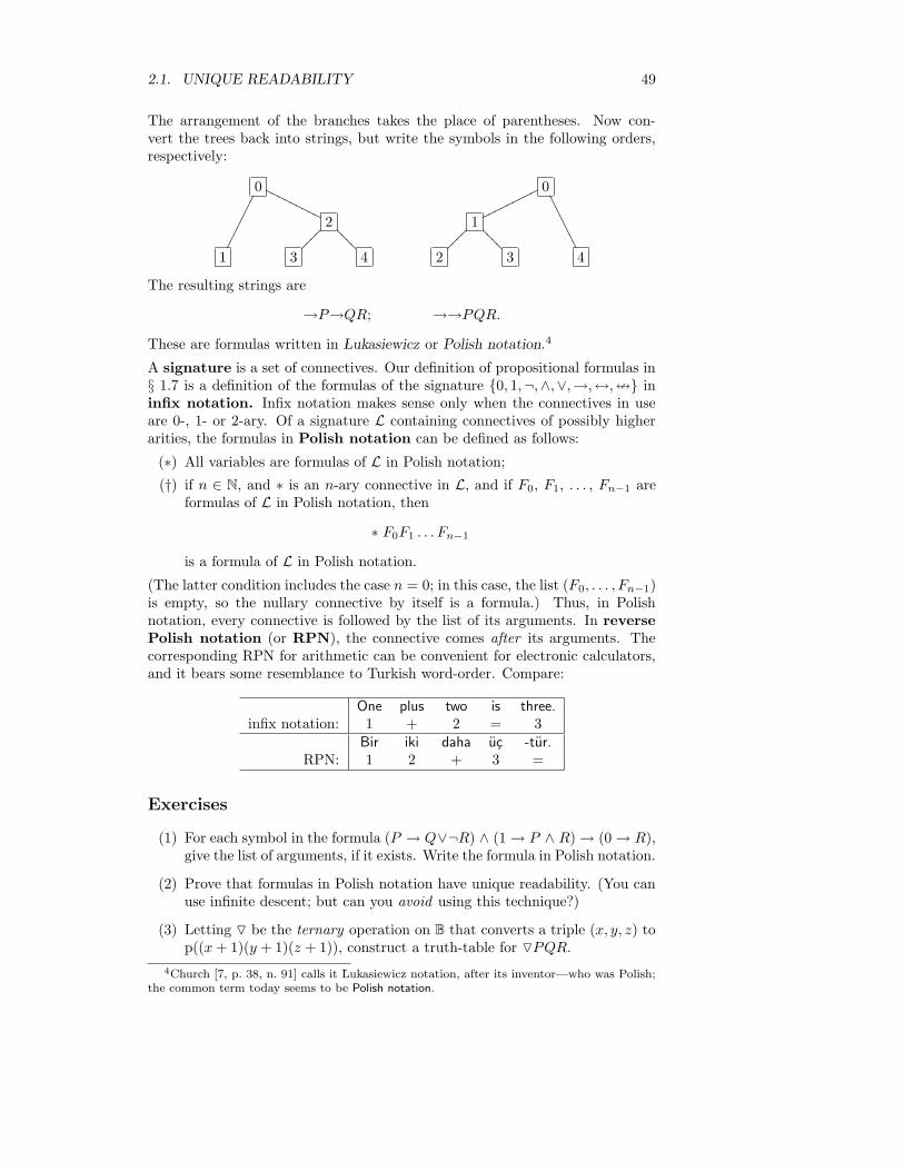
2.1. UNIQUE READABILITY 49
The arrangement of the branches takes the place of parentheses. Now con-vert the trees back into strings, but write the symbols in the following orders,respectively:
0
²²²²²²²² OOO
OOOOOO
2
ÄÄÄÄ ??
??
1 3 4
0
oooooo
ooo
////////
1
ÄÄÄÄ ??
??
2 3 4
The resulting strings are
→P→QR; →→PQR.
These are formulas written in ÃLukasiewicz or Polish notation.4
A signature is a set of connectives. Our definition of propositional formulas in§ 1.7 is a definition of the formulas of the signature 0, 1,¬,∧,∨,→,↔,= ininfix notation. Infix notation makes sense only when the connectives in useare 0-, 1- or 2-ary. Of a signature L containing connectives of possibly higherarities, the formulas in Polish notation can be defined as follows:
(∗) All variables are formulas of L in Polish notation;
(†) if n ∈ N, and ∗ is an n-ary connective in L, and if F0, F1, . . . , Fn−1 areformulas of L in Polish notation, then
∗ F0F1 . . . Fn−1
is a formula of L in Polish notation.
(The latter condition includes the case n = 0; in this case, the list (F0, . . . , Fn−1)is empty, so the nullary connective by itself is a formula.) Thus, in Polishnotation, every connective is followed by the list of its arguments. In reversePolish notation (or RPN), the connective comes after its arguments. Thecorresponding RPN for arithmetic can be convenient for electronic calculators,and it bears some resemblance to Turkish word-order. Compare:
One plus two is three.infix notation: 1 + 2 = 3
Bir iki daha uc -tur.RPN: 1 2 + 3 =
Exercises
(1) For each symbol in the formula (P → Q∨¬R) ∧ (1→ P ∧ R)→ (0→ R),give the list of arguments, if it exists. Write the formula in Polish notation.
(2) Prove that formulas in Polish notation have unique readability. (You canuse infinite descent; but can you avoid using this technique?)
(3) Letting O be the ternary operation on B that converts a triple (x, y, z) top((x+ 1)(y + 1)(z + 1)), construct a truth-table for OPQR.
4Church [7, p. 38, n. 91] calls it ÃLukasiewicz notation, after its inventor—who was Polish;the common term today seems to be Polish notation.
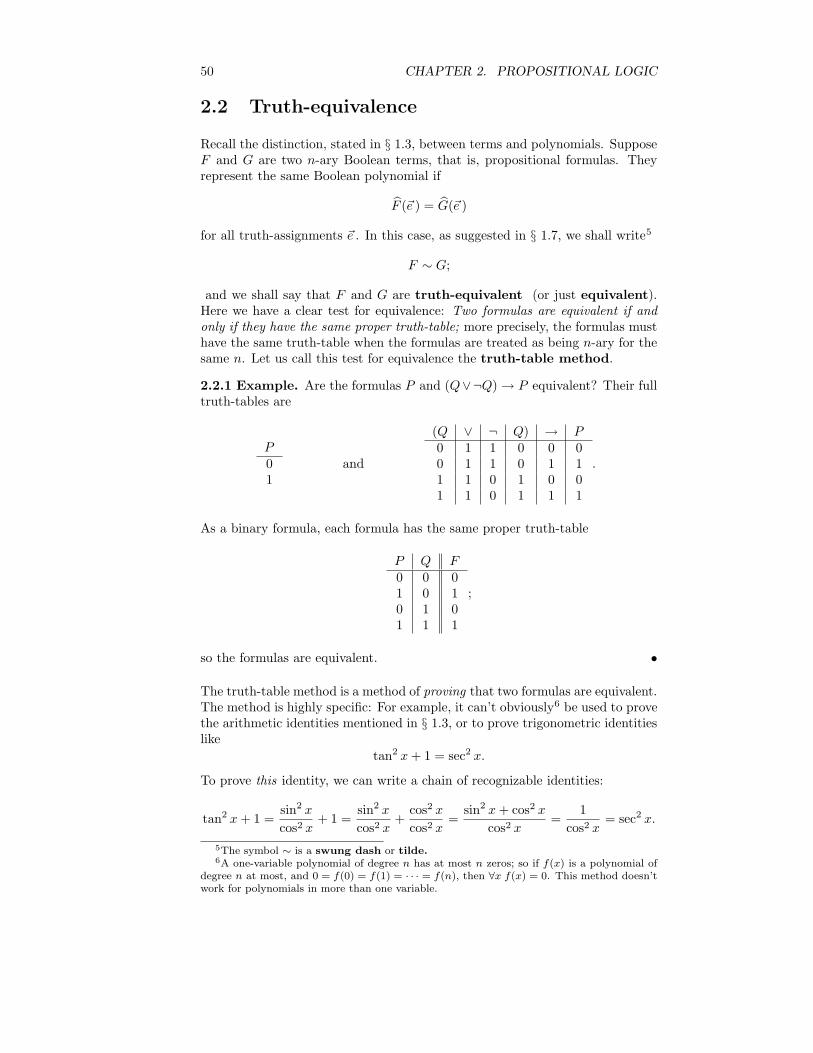
50 CHAPTER 2. PROPOSITIONAL LOGIC
2.2 Truth-equivalence
Recall the distinction, stated in § 1.3, between terms and polynomials. SupposeF and G are two n-ary Boolean terms, that is, propositional formulas. Theyrepresent the same Boolean polynomial if
F (~e ) = G(~e )
for all truth-assignments ~e . In this case, as suggested in § 1.7, we shall write5
F ∼ G;
and we shall say that F and G are truth-equivalent (or just equivalent).Here we have a clear test for equivalence: Two formulas are equivalent if andonly if they have the same proper truth-table; more precisely, the formulas musthave the same truth-table when the formulas are treated as being n-ary for thesame n. Let us call this test for equivalence the truth-table method.
2.2.1 Example. Are the formulas P and (Q∨¬Q)→ P equivalent? Their fulltruth-tables are
P01
and
(Q ∨ ¬ Q) → P0 1 1 0 0 00 1 1 0 1 11 1 0 1 0 01 1 0 1 1 1
.
As a binary formula, each formula has the same proper truth-table
P Q F0 0 01 0 10 1 01 1 1
;
so the formulas are equivalent. •
The truth-table method is a method of proving that two formulas are equivalent.The method is highly specific: For example, it can’t obviously6 be used to provethe arithmetic identities mentioned in § 1.3, or to prove trigonometric identitieslike
tan2 x+ 1 = sec2 x.
To prove this identity, we can write a chain of recognizable identities:
tan2 x+ 1 =sin2 x
cos2 x+ 1 =
sin2 x
cos2 x+
cos2 x
cos2 x=
sin2 x+ cos2 x
cos2 x=
1
cos2 x= sec2 x.
5The symbol ∼ is a swung dash or tilde.6A one-variable polynomial of degree n has at most n zeros; so if f(x) is a polynomial of
degree n at most, and 0 = f(0) = f(1) = · · · = f(n), then ∀x f(x) = 0. This method doesn’twork for polynomials in more than one variable.

2.2. TRUTH-EQUIVALENCE 51
This proof is an example of the method of simplification. This method canalso be used for propositional formulas. In this context, we shall develop thetheoretical background of simplification in the next section; the method itselfis developed in § 2.6. A proof by simplification, suitably expressed, will be anexample of a formal proof .
Meanwhile, the problem of checking for equivalence can be formulated in otherways. If F ∼ 1, then we write
² F (2.1)
and we say that F is a tautology.7 (The semantic turnstile ² was introduced in§ 1.9. To be consistent with the notation in that earlier section, we might writeLine (2.1) as B ² F ; but the variables in propositional formulas will always rangeover B.) If F ∼ 0, we call F a contradiction. We say F is satisfiable if it isnot a contradiction. If both F and ¬F are satisfiable, then F is a contingency.Hence, in the truth-table for F , if the column for F itself contains:
(∗) only 1s, then F is a tautology;
(†) only 0s, then F is a contradiction;
(‡) at least one 1, then F is satisfiable;
(§) at least one 1, and at least one 0, then F is a contingency.
Also, the following statements mean the same thing:
(∗) F ∼ G;
(†) ² F ↔ G;
(‡) ¬(F ↔ G) is not satisfiable.
Thus, in effect, a test for equivalence is a test for tautology is a test for satisfi-ability.
Exercises
(1) Test for the equivalence of the following pairs of formulas by the truth-table method:
(a) P and Q→ P ;
(b) P and Q→ (P ∧ Q);
(c) P → (Q→ R) and P → Q→ (P → R).
(2) Give examples of tautologies, contradictions, and contingencies.
(3) Establish the following equivalences by truth-tables (they will constituteLemma 2.6.1 below):
P → Q ∼ ¬P ∨Q;
P ↔ Q ∼ (P → Q) ∧ (Q→ P );
P = Q ∼ ¬(P ↔ Q);
¬¬P ∼ P ;
7From the Greek to aÎto, meaning the same. Originally a tautology was a redundantexpression, such as cease and desist.

52 CHAPTER 2. PROPOSITIONAL LOGIC
¬(P ∨Q) ∼ ¬P ∧ ¬Q; ¬(P ∧ Q) ∼ ¬P ∨ ¬Q;
P ∧ Q ∼ Q ∧ P ; P ∨Q ∼ Q ∨ P ;(P ∧ Q) ∧ R ∼ P ∧ Q ∧ R; (P ∨Q) ∨R ∼ P ∨Q ∨R;P ∧ (Q ∨R) ∼ (P ∧ Q) ∨ (P ∧ R); P ∨ (Q ∧ R) ∼ (P ∨Q) ∧ (P ∨R);
P ∧ P ∼ P ; P ∧ ¬P ∼ 0; P ∨ P ∼ P ; P ∨ ¬P ∼ 1;
P ∧ 1 ∼ P ; P ∧ 0 ∼ 0; P ∨ 0 ∼ P ; P ∨ 1 ∼ 1;
P ∼ (P ∧ Q) ∨ (P ∧ ¬Q); P ∼ (P ∨Q) ∧ (P ∨ ¬Q).
(4) Establish the following equivalences:
(a) ¬P ∼ 1 = P ;
(b) P ∨Q ∼ P = Q = P ∧ Q;
(c) P = Q ∼ Q = P ;
(d) (P = Q) = R ∼ P = Q = R;
(e) P ∧ (Q = R) ∼ P ∧ Q = P ∧ R;(f) P = P ∼ 0.
(5) Is there a formula F such that ² (F → (P ↔ Q)) ∧ (P ∨ (Q ∨ F ))?
2.3 Substitution and replacement
If F is a formula for which (e0, . . . , en−1) is a truth-assignment, then the constantformula F (e0, . . . , en−1) is obtained by substitution. In this substitution, it isnot essential that each ei be in the set B, that is, 0, 1; if (G0, . . . , Gn−1) is alist of n formulas, then from F we can obtain the formula
F (G0, . . . , Gn−1)
by substitution of Gj for each instance of Pj in F , for each j less than n. Notethat, if we are using the usual infix notation (see § 2.1), but have removedparentheses as allowed by our conventions, then the substitutions must be donewith parentheses as necessary to ensure that each substituted formula becomesa sub-formula of the new formula.
2.3.1 Example. Suppose F is P0 ∧ (P1 → P0), and G0 is P0 → P1, and G1 isP1 → (P0 ∨ P2). Then F (G0, G1) is
(P0 → P1) ∧ ((P1 → (P0 ∨ P2))→ (P0 → P1)). •
Substitution is associative in that, if we substitute some formulas Gi into F ,and then substitute some formulas Hj into the result, we get the same formulaas if we substitute the Hj first into the Gi, and then the results into F . Theformal statement is the following:

2.3. SUBSTITUTION AND REPLACEMENT 53
2.3.2 Lemma (Associativity). Suppose F is an n-ary formula, and
(G0, . . . , Gn−1)
is a list of n formulas, each `-ary. Let H be the formula F (G0, . . . , Gn−1). ThenH is `-ary. Suppose (K0, . . . ,K`−1) is a list of ` formulas. Then the formula
H(K0, . . . ,K`−1)
is the formula
F (G0(K0, . . . ,K`−1), . . . , Gn−1(K0, . . . ,K`−1)).
Finally, suppose ~e is a truth-assignment for the Gj. Then ~e is a truth-assign-ment for H. If also
Gj(~e ) = fj
for each j in 0, . . . , n− 1, then (f0, . . . , fn−1) is a truth-assignment ~f for F ,and
H(~e ) = F (~f ).
Proof. I claim that the proposition is obvious,8 in the sense that no writtenproof will make the truth of the proposition clearer than it already is to thereader who has understood the proposition.
Is a truth-assignment for F (G0, . . . , Gn−1) also a truth-assignment for the Gj?It is, if all of the variables P0, . . . , Pn−1 actually appear in F ; otherwise it maynot be:
2.3.3 Example. Suppose F is just P0, considered as a binary formula. Let Gi
be Pi when i ∈ 0, 1. Then F (G0, G1) is P0. Now, (0) is a truth-assignmentfor the formula P0; but (0) is not long enough to be a truth-assignment for G1.•2.3.4 Theorem (Substitution). If
F (P0, . . . , Pn−1) ∼ G(P0, . . . , Pn−1),
and (H0, . . . , Hn−1) is a list of n formulas, then
F (H0, . . . , Hn−1) ∼ G(H0, . . . , Hn−1).
Proof. Since F ∼ G, we have
F (~e ) = G(~e ) (2.2)
for all truth-assignments ~e for F and G. Let F ′ be F (H0, . . . , Hn−1), and let
G′ be G(H0, . . . , Hn−1). Suppose ~f is a truth-assignment for the Hj , and let
Hj(~f ) = ej . Then
F ′(~f ) = F (~e ) [by Lemma 2.3.2]
= G(~e ) [by Equation (2.2)]
= G′(~f ) [by Lemma 2.3.2].
8However, Church [7, § 15, p. 97] proves a version of this lemma by induction.

54 CHAPTER 2. PROPOSITIONAL LOGIC
Therefore F ′ ∼ G′. This completes the proof.9
2.3.5 Corollary. A tautology remains a tautology when arbitrary formulas aresubstituted for the variables.
Proof. Exercise.
2.3.6 Example. Since P ∨ ¬P is a tautology, so is (P → Q) ∨ ¬(P → Q). •
In ordinary language, substitution and replacement are nearly synonyms, al-though there is a distinction. From the expression abc, we get adc in a way thatcan be described in two ways:
(∗) by replacing b with d, or
(†) by substituting d for b.
When doing logic, we shall make another important distinction. If F is a sub-formula of G, then we may replace F with another formula F ′. Here, to replaceF is to replace a particular occurrence of F (since possibly F appears more thanonce as a sub-formula of G).
2.3.7 Example. In P ∨¬P , replacing the second occurrence of P with Q yieldsP ∨ ¬Q. •2.3.8 Theorem (Replacement). Suppose F is a sub-formula of G, and
F ∼ F ′.
Let G′ be the result of replacing F with F ′ in G. Then
G ∼ G′.
Proof. Say G is n-ary. Let H(P0, . . . , Pn) be the result of replacing F with Pnin G. Then G itself is the formula
H(P0, . . . , Pn−1, F ),
and G′ is H(P0, . . . , Pn−1, F′). The remainder of the proof10 is an exercise
involving Lemma 2.3.2.
2.3.9 Corollary. A tautology remains a tautology when a sub-formula is re-placed with an equivalent sub-formula.
Proof. Exercise.
2.3.10 Example. Since ² (P → Q) ∨ ¬(P → Q) by Example 2.3.6, and
¬(P → Q) ∼ P ∧ ¬Q,
we have ² (P → Q) ∨ (P ∧ ¬Q). •9This is also Burris’s proof [5, § 2.3, pp. 46f.], although Burris’s use of the fact given in
Lemma 2.3.2 is not entirely explicit.10Burris [5, § 2.4, pp. 48ff.] gives an elaborate proof using induction; but I think the work
is unnecessary, once one has Lemma 2.3.2. Church’s proof [7, § 15, p. 101] leaves details tothe reader, but also involves induction. Moreover, Church’s proof refers to the principle ofunique readability, which Burris seems not to discuss.

2.4. NORMAL FORMS 55
The Substitution and Replacement Theorems work together in the followingway. From known equivalences, Substitution lets us derive many more. ByReplacement, we can use these equivalences to write given formulas in different(but equivalent) form.
This, in short, is the method of simplification. Our first example of the proce-dure will be in § 2.5. Meanwhile, in § 2.4, we shall describe some formulas suchthat every formula is equivalent to one of them. These equivalences can be es-tablished by the procedure just described, once we have the stock of equivalencespresented in § 2.6.
Exercises
(1) If F (P ) is P → P → P , what is F (F (P ))?
(2) Prove Corollary 2.3.5.
(3) Prove Corollary 2.3.9.
2.4 Normal forms
If we have the truth-table of a formula, then we can read off an equivalentformula in so-called disjunctive normal form. The general procedure is describedimmediately, then illustrated by Example 2.4.1.
Suppose we have the truth-table for a formula F (P0, . . . , Pn−1). Say there arem rows in which the entry for F itself is 1. Then 0 6 m 6 2n. If we ignorethe other rows (namely, those rows in which the entry for F is 0), then whatremains has the form
P0 P1 . . . Pn−1 F
e00 e01 . . . e0n−1 1
e10 e11 . . . e1n−1 1...
......
...
em−10 em−1
1 . . . em−1n−1 1
where each eij is in B. (So, i is the row-number of eij in the truth-table, and j
is the column-number). If 0 6 i < m and 0 6 j < n, then let us define P ij to be
the formula ¬Pj , if eij = 0;
Pj , if eij = 1.
If 0 6 i < m, let Gi be the conjunction
P i0 ∧ · · · ∧ P i
n−1.
The formulas Gi can be called the normal disjunctive constituents of F .Their disjunction,
G0 ∨G1 ∨ · · · ∨Gm−1,

56 CHAPTER 2. PROPOSITIONAL LOGIC
is called a disjunctive normal form for F . (The other disjunctive normalforms for F are obtained by re-ordering the constituents Gi.) It is Theorem 2.4.3below that every formula is equivalent to its disjunctive normal forms.
Note here that we speak of conjunctions and disjunctions of arbitrarily manyformulas. The disjunction of the formulas H0, . . . , Hr−1 is
H0 ∨H1 ∨ · · · ∨Hr−1,
which can also be written ∨
i<r
Hi. (2.3)
If r = 1, then this formula is just H0. If r = 0, then, by convention,11 theformula (2.3) is understood to be 0. In particular, the disjunctive normal formof a contradiction is 0. The conjunction
∧
i<r
Hi
is defined analogously, and is 1 if r = 0.
2.4.1 Example. Here is the full truth-table of a particular disjunction:
¬ (P → Q) ∨ (R ∧ ¬ P )0 0 1 0 0 0 0 1 01 1 0 0 1 0 0 0 10 0 1 1 0 0 0 1 00 1 1 1 0 0 0 0 10 0 1 0 1 1 1 1 01 1 0 0 1 1 0 0 10 0 1 1 1 1 1 1 00 1 1 1 0 1 0 0 1
.
Extract the rows in which the column headed ∨ features 1, and take only oneeach of the columns for P , Q and R:
P Q R1 0 00 0 11 0 10 1 1
.
The disjunctive normal form for ¬(P → Q) ∨ (R ∧ ¬P ) is therefore
(P ∧ ¬Q ∧ ¬R) ∨ (¬P ∧ ¬Q ∧ R) ∨ (P ∧ ¬Q ∧ R) ∨ (¬P ∧ Q ∧ R). •
An n-ary formula is in disjunctive normal form if the formula is precisely
∨
i<m
∧
j<n
P ij ,
11The convention is reasonable: Instead of (2.3), we could writeWH0, . . . , Hr−1; infor-
mally, this says that at least one of the formulas Hi is true. If r = 0, then there are noformulas Hi, and in particular there is no such true formula, so
WH0, . . . , Hr−1 is false.

2.4. NORMAL FORMS 57
where each sub-formula P ij is either Pj or ¬Pj , but all of the constituents∧
j<n Pij are distinct. Note especially that each constituent must contain the
same variables.
2.4.2 Example. The formula ¬(P → Q) ∨ (R ∧ ¬P ) is equivalent to
(P ∧ ¬Q) ∨ (¬P ∧ ¬Q ∧ R) ∨ (¬P ∧ Q ∧ R),
but this is not a disjunctive normal form, since one of the constituents does notcontain R. •
2.4.3 Theorem. Every formula is equivalent to its disjunctive normal forms.
Proof. Let us use the notation of the definition above. Write H for∨i<mG
i.Then we have to show F ∼ H. For the truth-assignment (ei0, . . . , e
in−1), let us
write ~e i. For arbitrary truth-assignments ~f for the Gi, we have
Gi(~f ) =
1, if ~f = ~e i;
0, if ~f 6= ~e i.
Then
H(~f ) =
1, if ~f ∈ ~e 0, . . . , ~em−1;0, if ~f /∈ ~e 0, . . . , ~em−1.
Hence H and F have the same truth-table.
There is also a conjunctive normal form; it looks like the disjunctive form,except that the ∧ and the ∨ have switched roles. You read it off from the truth-table again, but you look for 0 (not 1) in the column for the formula, and P j
i
resolves to Pi if there is 0 in the corresponding column and row.
In particular, if a disjunctive form for an n-ary formula has m constituents, thena conjunctive form for the same formula will have 2n−m constituents. Whetherit is easier to work with the disjunctive or the conjunctive normal form dependson how big m is.
2.4.4 Example. To obtain the conjunctive normal form of the formula in Ex-ample 2.4.1, from its truth-table we extract
P Q R0 0 00 1 01 1 01 1 1
,
from which we read off
(P ∨Q ∨R) ∧ (P ∨ ¬Q ∨R) ∧ (¬P ∨ ¬Q ∨R) ∧ (¬P ∨ ¬Q ∨ ¬R). •
2.4.5 Theorem. Every formula is equivalent to its conjunctive normal form.
Proof. Exercise.
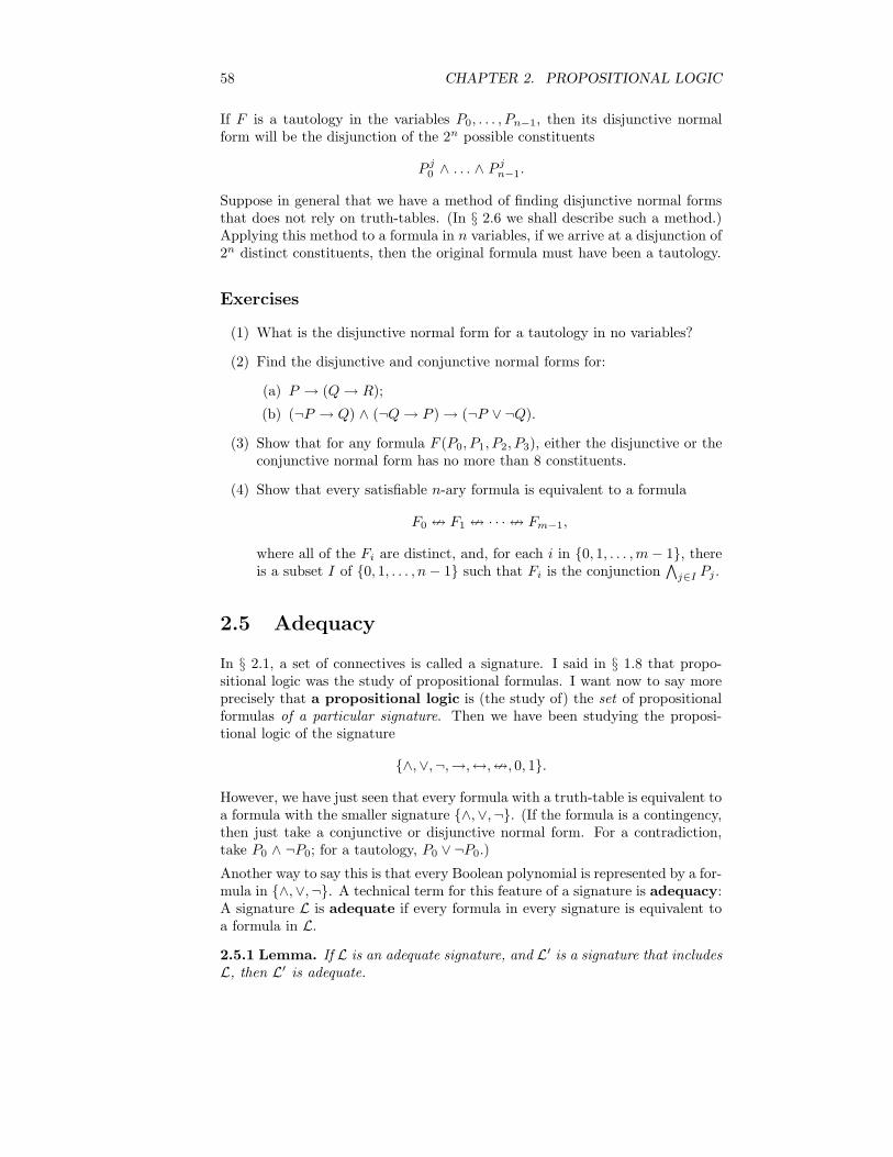
58 CHAPTER 2. PROPOSITIONAL LOGIC
If F is a tautology in the variables P0, . . . , Pn−1, then its disjunctive normalform will be the disjunction of the 2n possible constituents
P j0 ∧ . . . ∧ P j
n−1.
Suppose in general that we have a method of finding disjunctive normal formsthat does not rely on truth-tables. (In § 2.6 we shall describe such a method.)Applying this method to a formula in n variables, if we arrive at a disjunction of2n distinct constituents, then the original formula must have been a tautology.
Exercises
(1) What is the disjunctive normal form for a tautology in no variables?
(2) Find the disjunctive and conjunctive normal forms for:
(a) P → (Q→ R);
(b) (¬P → Q) ∧ (¬Q→ P )→ (¬P ∨ ¬Q).
(3) Show that for any formula F (P0, P1, P2, P3), either the disjunctive or theconjunctive normal form has no more than 8 constituents.
(4) Show that every satisfiable n-ary formula is equivalent to a formula
F0 = F1 = · · · = Fm−1,
where all of the Fi are distinct, and, for each i in 0, 1, . . . ,m− 1, thereis a subset I of 0, 1, . . . , n− 1 such that Fi is the conjunction
∧j∈I Pj .
2.5 Adequacy
In § 2.1, a set of connectives is called a signature. I said in § 1.8 that propo-sitional logic was the study of propositional formulas. I want now to say moreprecisely that a propositional logic is (the study of) the set of propositionalformulas of a particular signature. Then we have been studying the proposi-tional logic of the signature
∧,∨,¬,→,↔,=, 0, 1.
However, we have just seen that every formula with a truth-table is equivalent toa formula with the smaller signature ∧,∨,¬. (If the formula is a contingency,then just take a conjunctive or disjunctive normal form. For a contradiction,take P0 ∧ ¬P0; for a tautology, P0 ∨ ¬P0.)
Another way to say this is that every Boolean polynomial is represented by a for-mula in ∧,∨,¬. A technical term for this feature of a signature is adequacy:A signature L is adequate if every formula in every signature is equivalent toa formula in L.
2.5.1 Lemma. If L is an adequate signature, and L′ is a signature that includesL, then L′ is adequate.

2.5. ADEQUACY 59
Proof. Obvious.
In short, if a signature is adequate, then so is any larger signature.
In fact, there are proper subsets of ∧,∨,¬ that are adequate. The followingwas proved by Emil Post in 1921.12
2.5.2 Theorem. The signature ∨,¬ is adequate.
Proof. Since ∧,¬,∨ is adequate, it is enough to show that any formula inthis signature is equivalent to a formula in ∧,¬. Suppose F is in ∧,¬,∨.Every instance of ∧ in F determines (as in § 2.1) a sub-formula of F that is aconjunction. Say this conjunction is G ∧ H, where G and H are sub-formulasof F . We have an equivalence
P ∧ Q ∼ ¬(¬P ∨ ¬Q)
(as can be checked by truth-tables); therefore, by the Substitution Theorem, wehave
G ∧ H ∼ ¬(¬G ∨ ¬H).
By the Replacement Theorem, in F we can replace G ∧ H with ¬(¬G ∨ ¬H).In this way, we can remove all instances of ∧ from F , obtaining a formula in∨,¬ that is equivalent to F .
Similarly, we have:
2.5.3 Theorem. The signature ∧,¬ is adequate.
Proof. Exercise.
2.5.4 Corollary. The signature ∧,=, 1 is adequate.
Proof. The signature ∧,¬ is adequate, but the connective ¬ can be expressedin terms of = and 1, since
¬P ∼ 1 = P
by § 2.2, Exercise 4a; so ∧,=, 1 is adequate.
The proofs of the last three numbered propositions are examples of a generalmethod for proving adequacy of a signature L: Take a signature L′ that isknown to be adequate, and show that every connective in L′ can be expressedwith the connectives of L. Note well the two ingredients of the argument:
(∗) L′ is known to be adequate;
(†) the elements of L′ can be expressed in terms of L.12Post’s method is different from ours; see [32, pp. 167 f.].
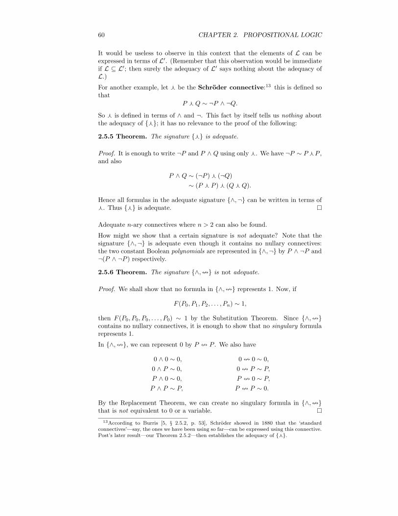
60 CHAPTER 2. PROPOSITIONAL LOGIC
It would be useless to observe in this context that the elements of L can beexpressed in terms of L′. (Remember that this observation would be immediateif L ⊆ L′; then surely the adequacy of L′ says nothing about the adequacy ofL.)For another example, let f be the Schroder connective:13 this is defined sothat
P fQ ∼ ¬P ∧ ¬Q.So f is defined in terms of ∧ and ¬. This fact by itself tells us nothing aboutthe adequacy of f; it has no relevance to the proof of the following:
2.5.5 Theorem. The signature f is adequate.
Proof. It is enough to write ¬P and P ∧ Q using only f. We have ¬P ∼ P fP ,and also
P ∧ Q ∼ (¬P )f (¬Q)
∼ (P f P )f (QfQ).
Hence all formulas in the adequate signature ∧,¬ can be written in terms off. Thus f is adequate.
Adequate n-ary connectives where n > 2 can also be found.
How might we show that a certain signature is not adequate? Note that thesignature ∧,¬ is adequate even though it contains no nullary connectives:the two constant Boolean polynomials are represented in ∧,¬ by P ∧ ¬P and¬(P ∧ ¬P ) respectively.
2.5.6 Theorem. The signature ∧,= is not adequate.
Proof. We shall show that no formula in ∧,= represents 1. Now, if
F (P0, P1, P2, . . . , Pn) ∼ 1,
then F (P0, P0, P0, . . . , P0) ∼ 1 by the Substitution Theorem. Since ∧,=contains no nullary connectives, it is enough to show that no singulary formularepresents 1.
In ∧,=, we can represent 0 by P = P . We also have
0 ∧ 0 ∼ 0, 0 = 0 ∼ 0,
0 ∧ P ∼ 0, 0 = P ∼ P,
P ∧ 0 ∼ 0, P = 0 ∼ P,
P ∧ P ∼ P, P = P ∼ 0.
By the Replacement Theorem, we can create no singulary formula in ∧,=that is not equivalent to 0 or a variable.
13According to Burris [5, § 2.5.2, p. 53], Schroder showed in 1880 that the ‘standardconnectives’—say, the ones we have been using so far—can be expressed using this connective.Post’s later result—our Theorem 2.5.2—then establishes the adequacy of f.

2.6. SIMPLIFICATION 61
Exercises
(1) Write down truth-tables for unknown formulas, and then find disjunctivenormal forms for those formulas.
(2) Prove Theorem 2.5.3.
(3) Prove that ¬,→ is adequate.
(4) Prove that ¬ by itself is not adequate.
(5) Prove the adequacy of the Sheffer stroke, the connective | such thatP | Q ∼ ¬ (P ∧ Q).
(6) Find an adequate ternary (3-ary) connective. (See § 2.1, Exercise 3.)
2.6 Simplification
In proving Theorem 2.5.2, we used a known equivalence, and the Theorems ofSubstitution and Replacement, to ‘simplify’ a formula in the sense of eliminatinginstances of disjunction. In the same way, we can simplify any formula to dis-junctive normal form. The procedure relies on the following lemma, which listssome fundamental properties of the Boolean connectives. (The label definitionshere is not a literal account of how the connectives were defined in § 1.7.)
2.6.1 Lemma.
(∗) definitions:
P → Q ∼ ¬P ∨Q,P ↔ Q ∼ (P → Q) ∧ (Q→ P ),
P = Q ∼ ¬(P ↔ Q);
(†) double negation:¬¬P ∼ P ;
(‡) De Morgan’s Laws:
¬(P ∨Q) ∼ ¬P ∧ ¬Q, ¬(P ∧ Q) ∼ ¬P ∨ ¬Q;
(§) Commutativity:
P ∧ Q ∼ Q ∧ P, P ∨Q ∼ Q ∨ P ;
(¶) Associativity:
(P ∧ Q) ∧ R ∼ P ∧ (Q ∧ R), (P ∨Q) ∨R ∼ P ∨ (Q ∨R);
(‖) Distributivity:
P ∧ (Q∨R) ∼ (P ∧ Q)∨ (P ∧ R), P ∨ (Q ∧ R) ∼ (P ∨Q) ∧ (P ∨R);

62 CHAPTER 2. PROPOSITIONAL LOGIC
(∗∗) redundancies:
P ∧ P ∼ P, P ∧ ¬P ∼ 0, P ∧ 1 ∼ P, P ∧ 0 ∼ 0,
P ∨ P ∼ P, P ∨ ¬P ∼ 1, P ∨ 0 ∼ P, P ∨ 1 ∼ 1;
(††) new variables:
P ∼ (P ∧ Q) ∨ (P ∧ ¬Q), P ∼ (P ∨Q) ∧ (P ∨ ¬Q).
Proof. This was § 2.2, Exercise 3.
To reduce a formula to disjunctive normal form, using the equivalences inLemma 2.6.1, we can:
(0) eliminate instances of →, ↔ and =;
(1) eliminate multiple negations, and make sure that the only arguments of ¬are variables;
(2) eliminate conjunctions of disjunctions;
(3) eliminate redundancies; now the formula is a disjunction of conjunctionsof variables and negated variables, so:
(4) add variables as necessary to obtain a disjunctive normal form.
2.6.2 Example. Suppose F is the formula ¬(P → Q) ∨ Q. The reduction ofF to disjunctive normal form can proceed as follows:
F ∼ ¬(¬P ∨Q) ∨Q [def’n of →]
∼ (¬¬P ∧ ¬Q) ∨Q [de Morgan]
∼ (P ∧ ¬Q) ∨Q [double negation]
∼ (P ∧ ¬Q) ∨ (Q ∧ P ) ∨ (Q ∧ ¬P ) [new variable]
∼ (P ∧ ¬Q) ∨ (P ∧ Q) ∨ (¬P ∧ Q) [commutativity] •
There may be more than one way to proceed:
2.6.3 Example. Let F be ¬(¬P → Q) ∧ (Q ∨ ¬P ). Then
F ∼ ¬(¬¬P ∨Q) ∧ (Q ∨ ¬P ) [def’n of →]
∼ ¬(P ∨Q) ∧ (Q ∨ ¬P ) [double neg.]
∼ (¬P ∧ ¬Q) ∧ (Q ∨ ¬P ) [De Morgan]
∼ ((¬P ∧ ¬Q) ∧ Q) ∨ ((¬P ∧ ¬Q) ∧ ¬P ) [dist.]
∼ (¬P ∧ (¬Q ∧ Q)) ∨ (¬P ∧ (¬P ∧ ¬Q)) [assoc.; comm.]
∼ (¬P ∧ 0) ∨ ((¬P ∧ ¬P ) ∧ ¬Q) [red.; assoc.]
∼ ¬P ∨ (¬P ∧ ¬Q) [red.]
∼ (¬P ∧ Q) ∨ (¬P ∧ ¬Q) ∨ (¬P ∧ ¬Q) [new var.]
∼ (¬P ∧ Q) ∨ (¬P ∧ ¬Q) [red.]
∼ ¬P. [new var.]
Thus, as a binary formula, F has the disjunctive normal form
(¬P ∧ Q) ∨ (¬P ∧ ¬Q);
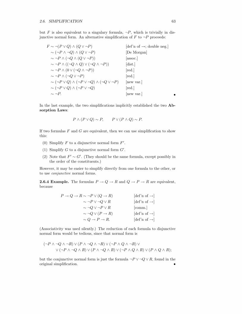
2.6. SIMPLIFICATION 63
but F is also equivalent to a singulary formula, ¬P , which is trivially in dis-junctive normal form. An alternative simplification of F to ¬P proceeds:
F ∼ ¬(P ∨Q) ∧ (Q ∨ ¬P ) [def’n of →; double neg.]
∼ (¬P ∧ ¬Q) ∧ (Q ∨ ¬P ) [De Morgan]
∼ ¬P ∧ (¬Q ∧ (Q ∨ ¬P )) [assoc.]
∼ ¬P ∧ ((¬Q ∧ Q) ∨ (¬Q ∧ ¬P )) [dist.]
∼ ¬P ∧ (0 ∨ (¬Q ∧ ¬P )) [red.]
∼ ¬P ∧ (¬Q ∨ ¬P ) [red.]
∼ (¬P ∨Q) ∧ (¬P ∨ ¬Q) ∧ (¬Q ∨ ¬P ) [new var.]
∼ (¬P ∨Q) ∧ (¬P ∨ ¬Q) [red.]
∼ ¬P. [new var.] •
In the last example, the two simplifications implicitly established the two Ab-sorption Laws:
P ∧ (P ∨Q) ∼ P, P ∨ (P ∧ Q) ∼ P.
If two formulas F and G are equivalent, then we can use simplification to showthis:
(0) Simplify F to a disjunctive normal form F ′.
(1) Simplify G to a disjunctive normal form G′.
(2) Note that F ′ ∼ G′. (They should be the same formula, except possibly inthe order of the constituents.)
However, it may be easier to simplify directly from one formula to the other, orto use conjunctive normal forms.
2.6.4 Example. The formulas P → Q → R and Q → P → R are equivalent,because
P → Q→ R ∼ ¬P ∨ (Q→ R) [def’n of →]
∼ ¬P ∨ ¬Q ∨R [def’n of →]
∼ ¬Q ∨ ¬P ∨R [comm.]
∼ ¬Q ∨ (P → R) [def’n of →]
∼ Q→ P → R. [def’n of →]
(Associativity was used silently.) The reduction of each formula to disjunctivenormal form would be tedious, since that normal form is
(¬P ∧ ¬Q ∧ ¬R) ∨ (P ∧ ¬Q ∧ ¬R) ∨ (¬P ∧ Q ∧ ¬R) ∨∨ (¬P ∧ ¬Q ∧ R) ∨ (P ∧ ¬Q ∧ R) ∨ (¬P ∧ Q ∧ R) ∨ (P ∧ Q ∧ R);
but the conjunctive normal form is just the formula ¬P ∨¬Q∨R, found in theoriginal simplification. •
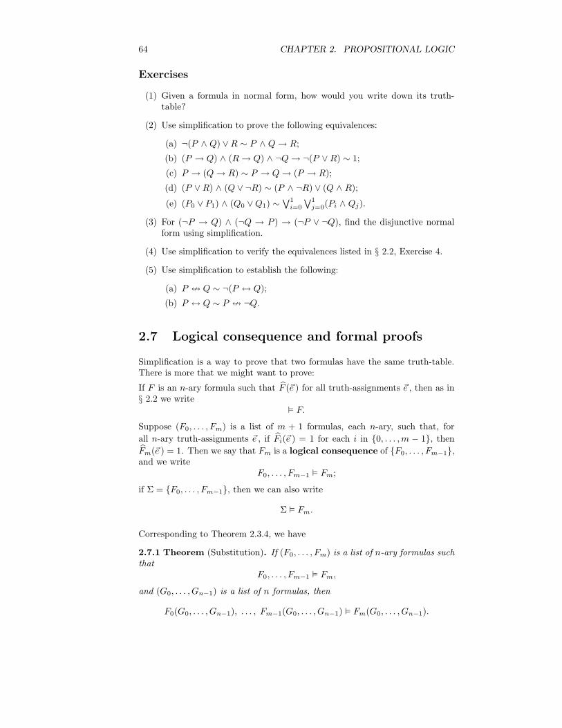
64 CHAPTER 2. PROPOSITIONAL LOGIC
Exercises
(1) Given a formula in normal form, how would you write down its truth-table?
(2) Use simplification to prove the following equivalences:
(a) ¬(P ∧ Q) ∨R ∼ P ∧ Q→ R;
(b) (P → Q) ∧ (R→ Q) ∧ ¬Q→ ¬(P ∨R) ∼ 1;
(c) P → (Q→ R) ∼ P → Q→ (P → R);
(d) (P ∨R) ∧ (Q ∨ ¬R) ∼ (P ∧ ¬R) ∨ (Q ∧ R);(e) (P0 ∨ P1) ∧ (Q0 ∨Q1) ∼
∨1i=0
∨1j=0(Pi ∧ Qj).
(3) For (¬P → Q) ∧ (¬Q → P ) → (¬P ∨ ¬Q), find the disjunctive normalform using simplification.
(4) Use simplification to verify the equivalences listed in § 2.2, Exercise 4.
(5) Use simplification to establish the following:
(a) P = Q ∼ ¬(P ↔ Q);
(b) P ↔ Q ∼ P = ¬Q.
2.7 Logical consequence and formal proofs
Simplification is a way to prove that two formulas have the same truth-table.There is more that we might want to prove:
If F is an n-ary formula such that F (~e ) for all truth-assignments ~e , then as in§ 2.2 we write
² F.
Suppose (F0, . . . , Fm) is a list of m + 1 formulas, each n-ary, such that, for
all n-ary truth-assignments ~e , if Fi(~e ) = 1 for each i in 0, . . . ,m − 1, thenFm(~e ) = 1. Then we say that Fm is a logical consequence of F0, . . . , Fm−1,and we write
F0, . . . , Fm−1 ² Fm;
if Σ = F0, . . . , Fm−1, then we can also write
Σ ² Fm.
Corresponding to Theorem 2.3.4, we have
2.7.1 Theorem (Substitution). If (F0, . . . , Fm) is a list of n-ary formulas suchthat
F0, . . . , Fm−1 ² Fm,
and (G0, . . . , Gn−1) is a list of n formulas, then
F0(G0, . . . , Gn−1), . . . , Fm−1(G0, . . . , Gn−1) ² Fm(G0, . . . , Gn−1).

2.7. LOGICAL CONSEQUENCE AND FORMAL PROOFS 65
Proof. Write the Fi(G0, . . . , Gn−1) asHi. Say ~e is a truth-assignment for the Gj
such that Hi(~e ) = 1 when i < m. Let fj = Gi(~e ) when j < n. Then Fi(~f ) = 1when i < m, by the associativity of substitution (that is, Lemma 2.3.2). Hence
also Hm(~e ) = Fm(~f ) = 1 (since Fm is a logical consequence of F0, . . . , Fm−1),so H0, . . . , Hm−1 ² Hm, which was to be proved.
The following basic means of establishing logical consequence should be com-pared with Implication (1.21):
2.7.2 Lemma (Detachment). F, F → G ² G.
Proof. It is enough to show P0, P0 → P1 ² P1, by the preceding SubstitutionTheorem. The truth-table
P0 P0 → P1 P1
0 0 1 0 01 1 0 0 00 0 1 1 11 1 1 1 1
shows that (1, 1) is the only truth-assignment where both P0 and P0 → P1 aretrue. Under this assignment, P1 is true.
Suppose F is a formula, and Σ is a set of formulas. A deduction or formalproof of F from Σ is a finite non-empty list
G0, . . . , G`
of formulas such that G` is F , and for each k in 0, . . . , `, one of the followingconditions is met:
(∗) Gk is in Σ; or
(†) Gk is a tautology; or
(‡) there is j in 0, . . . , k − 1 such that Gj ∼ Gk; or
(§) there are distinct i and j in 0, . . . , k − 1 such that Gj is Gi → Gk.
If such a deduction exists, then we say that F is deducible or formally prov-able from Σ, and Σ is a set of hypotheses (singular: hypothesis) from whichF is deducible; we may then write
Σ ` F.
If Σ is a finite set G0, . . . , Gm−1, then we can also write G0, . . . , Gm−1 ` F ;if Σ is empty, we write
` F.
2.7.3 Example. F ∧ G ` G, because the following is a deduction of G fromF ∧ G:
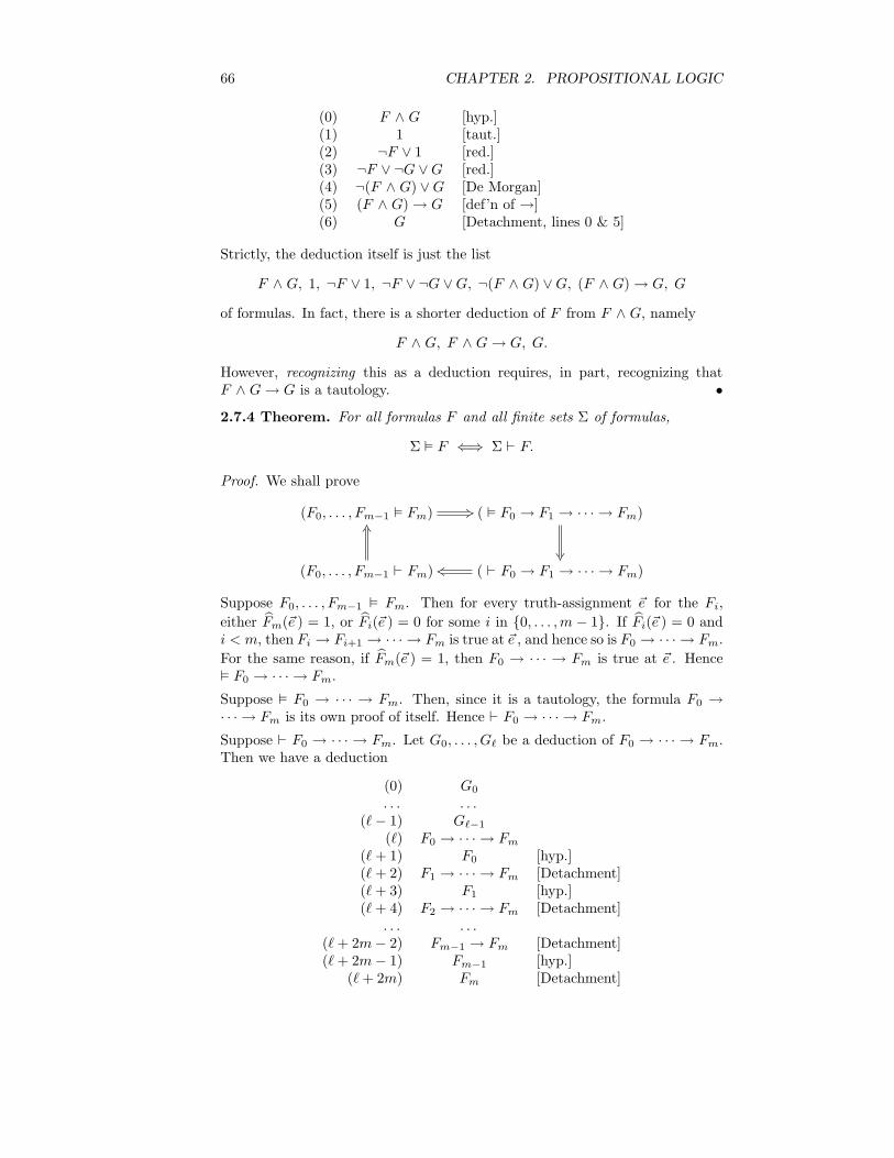
66 CHAPTER 2. PROPOSITIONAL LOGIC
(0) F ∧ G [hyp.](1) 1 [taut.](2) ¬F ∨ 1 [red.](3) ¬F ∨ ¬G ∨G [red.](4) ¬(F ∧ G) ∨G [De Morgan](5) (F ∧ G)→ G [def’n of →](6) G [Detachment, lines 0 & 5]
Strictly, the deduction itself is just the list
F ∧ G, 1, ¬F ∨ 1, ¬F ∨ ¬G ∨G, ¬(F ∧ G) ∨G, (F ∧ G)→ G, G
of formulas. In fact, there is a shorter deduction of F from F ∧ G, namely
F ∧ G, F ∧ G→ G, G.
However, recognizing this as a deduction requires, in part, recognizing thatF ∧ G→ G is a tautology. •2.7.4 Theorem. For all formulas F and all finite sets Σ of formulas,
Σ ² F ⇐⇒ Σ ` F.
Proof. We shall prove
(F0, . . . , Fm−1 ² Fm) +3 ( ² F0 → F1 → · · · → Fm)
®¶(F0, . . . , Fm−1 ` Fm)
KS
( ` F0 → F1 → · · · → Fm)ks
Suppose F0, . . . , Fm−1 ² Fm. Then for every truth-assignment ~e for the Fi,
either Fm(~e ) = 1, or Fi(~e ) = 0 for some i in 0, . . . ,m − 1. If Fi(~e ) = 0 andi < m, then Fi → Fi+1 → · · · → Fm is true at ~e , and hence so is F0 → · · · → Fm.
For the same reason, if Fm(~e ) = 1, then F0 → · · · → Fm is true at ~e . Hence² F0 → · · · → Fm.
Suppose ² F0 → · · · → Fm. Then, since it is a tautology, the formula F0 →· · · → Fm is its own proof of itself. Hence ` F0 → · · · → Fm.
Suppose ` F0 → · · · → Fm. Let G0, . . . , G` be a deduction of F0 → · · · → Fm.Then we have a deduction
(0) G0
. . . . . .(`− 1) G`−1
(`) F0 → · · · → Fm(`+ 1) F0 [hyp.](`+ 2) F1 → · · · → Fm [Detachment](`+ 3) F1 [hyp.](`+ 4) F2 → · · · → Fm [Detachment]
. . . . . .(`+ 2m− 2) Fm−1 → Fm [Detachment](`+ 2m− 1) Fm−1 [hyp.]
(`+ 2m) Fm [Detachment]

2.7. LOGICAL CONSEQUENCE AND FORMAL PROOFS 67
of Fm from F0, . . . , Fm−1. Thus F0, . . . , Fm−1 ` Fm.
Suppose finally F0, . . . , Fm−1 ` Fm. We use the method of infinite descent.Let G0, . . . , G`−1, Fm be a deduction of Fm from F0, . . . , Fm−1. Let ~e be a
truth-assignment such that Fi(~e ) = 1 whenever i < m. Suppose if possible that
Fm(~e ) = 0. Then Fm is not in F0, . . . , Fm−1, nor is Fm a tautology. Hence,by the definition of a deduction, either Fm ∼ Gi for some i in 0, . . . , ` − 1,or there are i and j in 0, . . . , ` − 1 such that Gj is Gi → Fm. In the firstcase, Gi is false at ~e ; in the second case, either Gi or Gj is false at ~e . In either
case, Gk(~e ) = 0 for some k in 0, . . . , `− 1. But G0, . . . , Gk is still a deductionfrom F0, . . . , Fm−1, strictly shorter then the original one, but with the sameproperty (namely that its last formula is false at ~e ). We can’t take shorter
deductions indefinitely. Hence Fm(~e ) = 1. Therefore F0, . . . , Fm−1 ² Fm.
Suppose F0, . . . , Fm−1 ² Fm. The proof of the last theorem shows how to writedown a deduction of Fm from F0, . . . , Fm−1. Indeed, let G0 be the formulaF0 → F1 → · · · → Fm. Then G0 must be a tautology, so the sequence
G0, F0, F1 → · · · → Fm, F1, F2 → · · · → Fm, . . . , Fm
is a deduction from F0, . . . , Fm−1. The problem is that this sequence is notobviously a deduction. To make it so, we can apply simplification to G0, gettinga chain
G0 ∼ G1 ∼ · · · ∼ G`
of equivalences as in § 2.6, where G` is a tautology in disjunctive or conjunctivenormal form (or follows from such a tautology by a substitution). Then thesequence
G`, G`−1, . . . , G0, F0, F1 → · · · → Fm, F1, F2 → · · · → Fm, . . . , Fm (2.4)
will be a deduction, and recognizably so; we may call it a recognizable de-duction. I’m not giving a precise definition of recognizable. It could be done,but we might find the definition too restrictive. Informally then, recognizablededuction is:
(∗) a deduction;
(†) clearly a deduction to any reader that knows the rules of simplificationestablished in § 2.6.
Not every recognizable deduction need be as long as the Deduction (2.4); theremay be short-cuts:
2.7.5 Example. To show F ∨G, ¬F ` G, we can start with the simplification
F ∨G→ ¬F → G ∼ ¬(F ∨G) ∨ (¬F → G)
∼ ¬(F ∨G) ∨ (F ∨G)
ending in a tautology derived from ¬P ∨P by substitution. Then the sequence
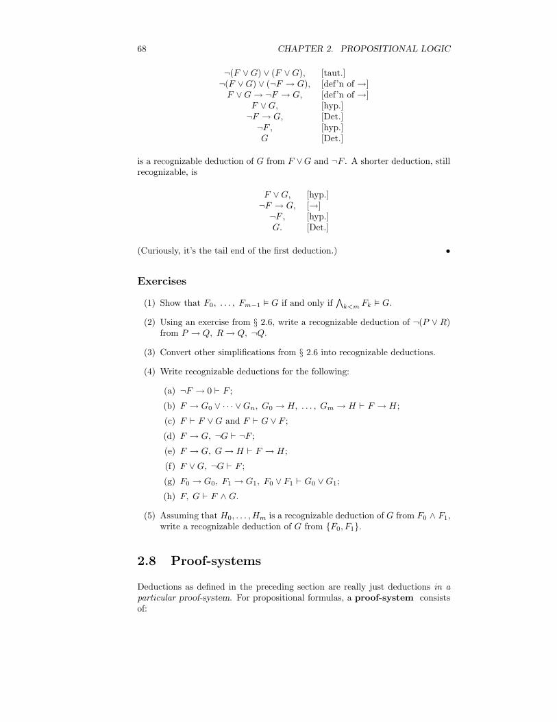
68 CHAPTER 2. PROPOSITIONAL LOGIC
¬(F ∨G) ∨ (F ∨G), [taut.]¬(F ∨G) ∨ (¬F → G), [def’n of →]F ∨G→ ¬F → G, [def’n of →]
F ∨G, [hyp.]¬F → G, [Det.]¬F , [hyp.]G [Det.]
is a recognizable deduction of G from F ∨G and ¬F . A shorter deduction, stillrecognizable, is
F ∨G, [hyp.]¬F → G, [→]¬F , [hyp.]G. [Det.]
(Curiously, it’s the tail end of the first deduction.) •
Exercises
(1) Show that F0, . . . , Fm−1 ² G if and only if∧k<m Fk ² G.
(2) Using an exercise from § 2.6, write a recognizable deduction of ¬(P ∨ R)from P → Q, R→ Q, ¬Q.
(3) Convert other simplifications from § 2.6 into recognizable deductions.
(4) Write recognizable deductions for the following:
(a) ¬F → 0 ` F ;(b) F → G0 ∨ · · · ∨Gn, G0 → H, . . . , Gm → H ` F → H;
(c) F ` F ∨G and F ` G ∨ F ;(d) F → G, ¬G ` ¬F ;(e) F → G, G→ H ` F → H;
(f) F ∨G, ¬G ` F ;(g) F0 → G0, F1 → G1, F0 ∨ F1 ` G0 ∨G1;
(h) F, G ` F ∧ G.
(5) Assuming that H0, . . . , Hm is a recognizable deduction of G from F0 ∧ F1,write a recognizable deduction of G from F0, F1.
2.8 Proof-systems
Deductions as defined in the preceding section are really just deductions in aparticular proof-system. For propositional formulas, a proof-system consistsof:

2.8. PROOF-SYSTEMS 69
(∗) axioms14, that is, certain distinguished formulas, and
(†) rules of inference, which are clearly described ways of obtaining newformulas from finitely many given formulas.
Then, of the proof-system of § 2.7,(∗) the axioms are just the tautologies;
(†) the rules of inference are two:
(0) to infer, from any formula, a formula equivalent to it;
(1) (also called Modus Ponens): to infer, from F and F → G, theformula G.
Then the following should be an obvious generalization of what we did in § 2.7:Suppose we have a proof-system N and a list (F0, . . . , Fm) of formulas. In thesystem N , a deduction or formal proof of Fm from F0, . . . , Fm−1 is a finitesequence
G0, . . . , G`,
where G` is Fm and, for each k in 0, . . . , `, the formula Gk is:
(∗) an axiom of N , or
(†) one of the formulas Fi, where i < m, or
(‡) a formula obtainable from (some of) the formulas in G0, . . . , Gk−1 byone of the rules of inference of N .
If there is such a deduction, then we write
F0, . . . , Fm−1 `N Fm,
and we say that Fm is derivable or formally provable in N from the setF0, . . . , Fm−1 of hypotheses. In case m = 0, we write `N F0 and say thatF0 is a validity of N (or a theorem of N ).
We might think of axioms as rules of inference whereby certain formulas can beinferred from no given formulas.
Many proof-systems are possible. Some are more useful than others. As aminimum requirement, we should like a proof-system N to have the followingtwo properties:
(∗) soundness: if F0, . . . , Fn−1 `N G, then F0, . . . , Fn−1 ² G;
(†) completeness: if F0, . . . , Fn−1 ² G, then F0, . . . , Fn−1 `N G.
Theorem 2.7.4 is that the proof-system of § 2.7 is sound and complete.
In § 2.7, the notion of a recognizable deduction was kept imprecise. The Substi-tution Theorem 2.7.1 gives a way to add new rules of inference to our system,some of which we may want to allow in recognizable deductions. For instance,taking note of Example 2.7.3, we may want to allow the rule of inferring G fromF ∧ G. More generally, if we know
F0, . . . , Fm−1 ² Fm,
14From the Greek ĆxÐwma, Ćxiÿmatoc (honor, worth, etc.).

70 CHAPTER 2. PROPOSITIONAL LOGIC
then we may allow the rule of inferring Fm(G0, . . . , Gn−1) from the formulas
F0(G0, . . . , Gn−1), . . . , Fm−1(G0, . . . , Gn−1),
for every list (G0, . . . , Gn−1) of n formulas.
In any case, we have the rule that, from a formula, we may derive an equivalentformula. This is not a rule of inference such as we have just described. ButDetachment is such a rule, being derived from
P, P → Q ² Q.
More rules can be obtained from the following:
2.8.1 Lemma.
(∗) ¬P → 0 ² P (Contradiction);
(†) P ∧ Q ² Q;(‡) P → Q0 ∨ · · · ∨Qn, Q0 → R, . . . , Qm → R ² P → R (Cases);
(§) P ² P ∨Q and P ² Q ∨ P (Addition);
(¶) P → Q, ¬Q ² ¬P (Modus Tollens15);
(‖) P → Q, Q→ R ² P → R (Hypothetical Syllogism16);
(∗∗) P ∨Q, ¬P ² Q and P ∨Q, ¬Q ² P (Disjunctive Syllogism);
(††) P0 → Q0, P1 → Q1, P0 ∨ P1 ² Q0 ∨Q1 (Constructive Dilemma).
Proof. These were all proved in § 1.4 (most as exercises).
Exercises
Write deductions for the following, using Lemma 2.8.1:
(1) P ↔ Q, Q↔ R ` P ↔ R;
(2) P = Q, Q = R ` P ↔ R.
2.9 ÃLukasiewicz’s proof system
Here is developed a proof-system L (for its inventor ÃLukasiewicz). It is of interestfor the simplicity of its definition. It involves only formulas in the signature→,¬. (We know from an exercise in § 2.5 that this signature is adequate.)The only rule of inference of L is Detachment. The axioms of L are of threekinds17:
15Latin for method [of] denying.16A syllogism is a classical form of argument; Aristotle’s definition is quoted in Appendix A.
A standard example of a syllogism is: All men are mortal. Socrates is a man. Therefore Socratesis mortal.
17Frege had an earlier proof-system in this signature that used three additional kinds ofaxioms.

2.9. ÃLUKASIEWICZ’S PROOF SYSTEM 71
(0) `L F → G→ F (Affirmation of the Consequent);
(1) `L (F → G → H) → (F → G) → F → H (Self-Distributivity ofImplication);
(2) `L (¬F → ¬G)→ G→ F (Contraposition).
System L is sound by Lemma 2.7.2 and because the axioms are tautologies. Toprove completeness, we shall need the following.
2.9.1 Lemma. `L F → F .
Proof. The formal proof is
F → F → F
F → (F → F )→ F
(F → (F → F )→ F )→ (F → F → F )→ F → F
(F → F → F )→ F → F
F → F,
where the first three entries are axioms (0), (0), and (1) respectively, and thelast two follow by Detachment.
2.9.2 Lemma. If F0, . . . , Fn−1 `L G→ H, then F0, . . . , Fn−1, G `L H.
Proof. Exercise.
The converse of Lemma 2.9.2 is the following; the proof is by cases (and themethod of infinite descent).
2.9.3 Theorem (Deduction). If F0, . . . , Fn−1, G `L H, then
F0, . . . , Fn−1 `L G→ H.
Proof. There are three possibilities for H:
If H is an axiom of L, or is one of the formulas Fi, then F0, . . . , Fn−1 `L H;but also `L H → G→ H; hence F0, . . . , Fn−1 `L G→ H by Detachment.
If H is G, then `L G→ H by Lemma 2.9.1.
Finally, suppose K0, . . . ,Km is the formal proof in L of H from F0, . . . , Fn−1
and G, and suppose the last step in the proof is by Detachment. (If it’s not,then we have already treated this possibility.) Then Ki is F , and Kj is F → H,for some formula F , and for some i and j less than m. If G→ Ki and G→ Kj
can be deduced in L from F0, . . . , Fn−1, then, by Detachment and the Self-Distributivity Axiom, so can G → H. Also, both Ki and Kj have shorterdeductions than H in L. Hence, if G → H cannot be deduced, then neithercan G → K for some K with a shorter deduction than H, which would beabsurd.
2.9.4 Lemma. The following are validities of L:
(1) ¬G→ G→ F ;
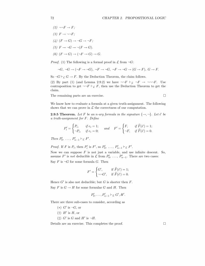
72 CHAPTER 2. PROPOSITIONAL LOGIC
(2) ¬¬F → F ;
(3) F → ¬¬F ;
(4) (F → G)→ ¬G→ ¬F ;
(5) F → ¬G→ ¬(F → G).
(6) (F → G)→ (¬F → G)→ G.
Proof. (1) The following is a formal proof in L from ¬G:
¬G, ¬G→ (¬F → ¬G), ¬F → ¬G, ¬F → ¬G→ (G→ F ), G→ F.
So ¬G `L G→ F . By the Deduction Theorem, the claim follows.
(2) By part (1) (and Lemma 2.9.2) we have ¬¬F `L ¬F → ¬¬¬F . Usecontraposition to get ¬¬F `L F , then use the Deduction Theorem to get theclaim.
The remaining parts are an exercise.
We know how to evaluate a formula at a given truth-assignment. The followingshows that we can prove in L the correctness of our computation.
2.9.5 Theorem. Let F be an n-ary formula in the signature →,¬. Let ~e bea truth-assignment for F . Define
P ′i =
Pi, if ei = 1;
¬Pi, if ei = 0;and F ′ =
F, if F (~e ) = 1;
¬F, if F (~e ) = 0.
Then P ′0, . . . , P′n−1 `L F ′.
Proof. If F is Pi, then P′i is F ′, so P ′0, . . . , P
′n−1 `L F ′.
Now we can suppose F is not just a variable, and use infinite descent. So,assume F ′ is not deducible in L from P ′0, . . . , P
′n−1. There are two cases:
Say F is ¬G for some formula G. Then
F ′ =
G′, if F (~e ) = 1;
¬¬G′, if F (~e ) = 0.
Hence G′ is also not deducible; but G is shorter then F .
Say F is G→ H for some formulas G and H. Then
P ′0, . . . , P′n−1 `L G′, H ′.
There are three sub-cases to consider, according as
(∗) G′ is ¬G, or(†) H ′ is H, or
(‡) G′ is G and H ′ is ¬H.
Details are an exercise. This completes the proof.
2.9. ÃLUKASIEWICZ’S PROOF SYSTEM 73
2.9.6 Corollary. The proof-system L is complete.
Proof. Suppose F0, . . . , Fm−1 ² Fm, the formulas being n-ary. Let G be thetautology F0 → · · · → Fm. Then for all n-ary truth-assignments ~e , we have
P ′0 . . . , P′n−1 `L G.
If n = 0, we are done. If n > 0, then by the Deduction Theorem we have
P ′0 . . . , P′n−2 `L Pn−1 → G,¬Pn−1 → G,
so P ′0 . . . , P′n−2 `L G by Lemma 2.9.4 (6). Continuing, we find `L G, so
F0, . . . , Fm−1 `L Fm.
Exercises
(1) Prove Lemma 2.9.2.
(2) Prove parts (3), (4), (5) and (6) of Lemma 2.9.4.
(3) Supply the missing details in the proof of Theorem 2.9.5.
Chapter 3
Sets and Relations
3.0 Boolean operations on sets
As observed in § 1.8, propositional logic is a model of the use of conjunctionsin ordinary language. A basic application of propositional logic is to sets.
Suppose U is some large set—a universal set, which will include all of theother sets that we shall work with. By the Axiom of Comprehension, 1.2.3, ifP is a predicate applying (truly or falsely) to the elements of U , then we canform a set
x ∈ U : Px. (3.1)
We have not yet said much about what P might be. Now we do.
If A ⊆ U and c ∈ U , then we can form the proposition
c ∈ A,
which is either true or false. We can analyze this proposition into two parts:
c ∈ Asubject predicate
With the predicate ∈ A and an individual variable, x, we can make theformula
x ∈ A.This is not a propositional formula, since ∈ is not a symbol of propositionallogic. Let us call the formula a set-theoretic formula or an ∈-formula. Wemay replace the set A with other sets, but for now, our only individual variablewill be x. (We shall allow more variables in § 3.2.)First note that we can write A as
x ∈ U : x ∈ A
(the set of x in U such that x is in A). This is not very interesting; but we cancreate more interest by combining ∈-formulas, by means of Boolean connectives,
74
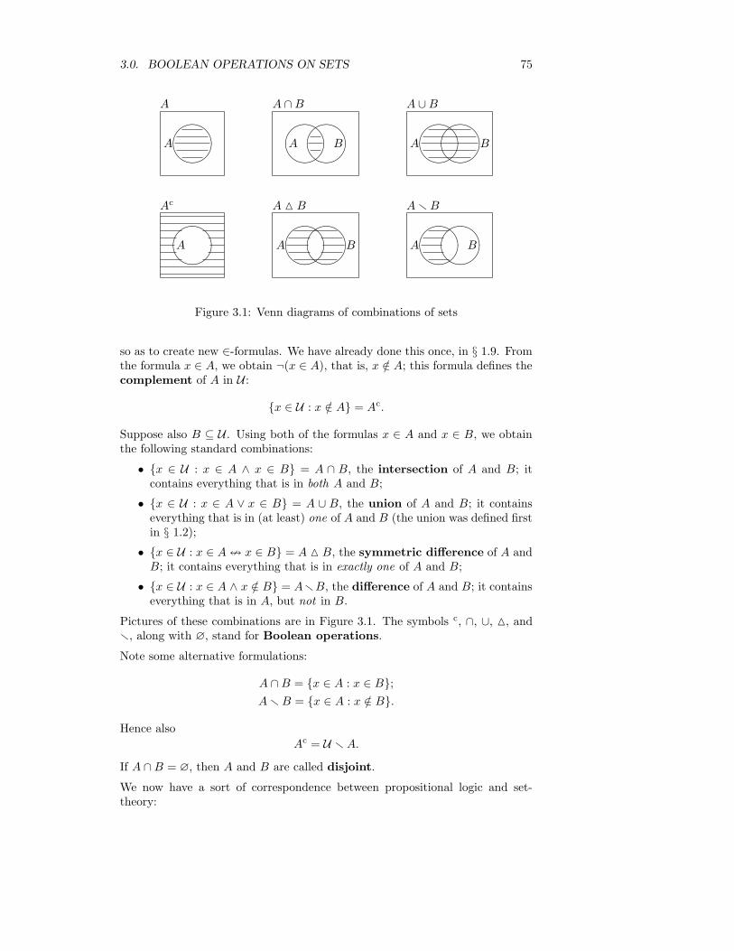
3.0. BOOLEAN OPERATIONS ON SETS 75
A
AÁÀ¿ A ∩B
A BÁÀ¿ÁÀ¿ A ∪B
A BÁÀ¿ÁÀ¿
Ac
AÁÀ¿ A M B
A BÁÀ¿ÁÀ¿ ArB
A BÁÀ¿ÁÀ¿
Figure 3.1: Venn diagrams of combinations of sets
so as to create new ∈-formulas. We have already done this once, in § 1.9. Fromthe formula x ∈ A, we obtain ¬(x ∈ A), that is, x /∈ A; this formula defines thecomplement of A in U :
x ∈ U : x /∈ A = Ac.
Suppose also B ⊆ U . Using both of the formulas x ∈ A and x ∈ B, we obtainthe following standard combinations:
• x ∈ U : x ∈ A ∧ x ∈ B = A ∩ B, the intersection of A and B; itcontains everything that is in both A and B;
• x ∈ U : x ∈ A ∨ x ∈ B = A ∪ B, the union of A and B; it containseverything that is in (at least) one of A and B (the union was defined firstin § 1.2);
• x ∈ U : x ∈ A = x ∈ B = A M B, the symmetric difference of A andB; it contains everything that is in exactly one of A and B;
• x ∈ U : x ∈ A ∧ x /∈ B = ArB, the difference of A and B; it containseverything that is in A, but not in B.
Pictures of these combinations are in Figure 3.1. The symbols c, ∩, ∪, M, andr, along with ∅, stand for Boolean operations.
Note some alternative formulations:
A ∩B = x ∈ A : x ∈ B;ArB = x ∈ A : x /∈ B.
Hence also
Ac = U rA.
If A ∩B = ∅, then A and B are called disjoint.
We now have a sort of correspondence between propositional logic and set-theory:
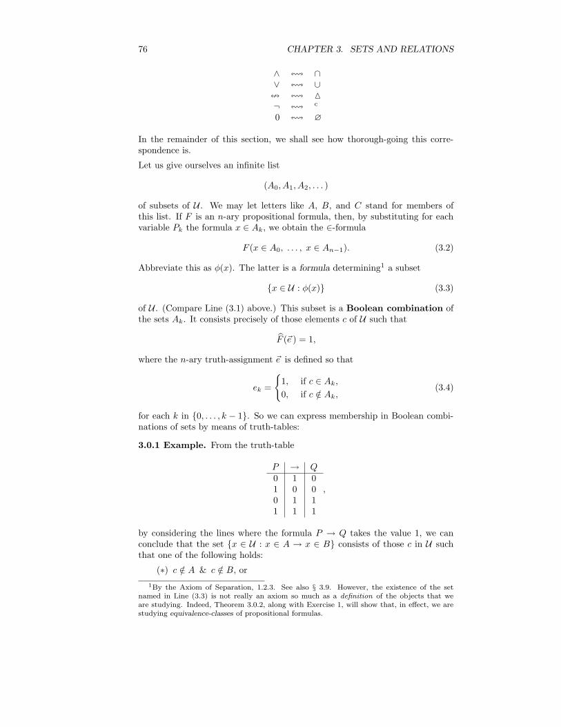
76 CHAPTER 3. SETS AND RELATIONS
∧ ! ∩∨ ! ∪
= ! M
¬ ! c
0 ! ∅
In the remainder of this section, we shall see how thorough-going this corre-spondence is.
Let us give ourselves an infinite list
(A0, A1, A2, . . . )
of subsets of U . We may let letters like A, B, and C stand for members ofthis list. If F is an n-ary propositional formula, then, by substituting for eachvariable Pk the formula x ∈ Ak, we obtain the ∈-formula
F (x ∈ A0, . . . , x ∈ An−1). (3.2)
Abbreviate this as φ(x). The latter is a formula determining1 a subset
x ∈ U : φ(x) (3.3)
of U . (Compare Line (3.1) above.) This subset is a Boolean combination ofthe sets Ak. It consists precisely of those elements c of U such that
F (~e ) = 1,
where the n-ary truth-assignment ~e is defined so that
ek =
1, if c ∈ Ak,
0, if c /∈ Ak,(3.4)
for each k in 0, . . . , k − 1. So we can express membership in Boolean combi-nations of sets by means of truth-tables:
3.0.1 Example. From the truth-table
P → Q0 1 01 0 00 1 11 1 1
,
by considering the lines where the formula P → Q takes the value 1, we canconclude that the set x ∈ U : x ∈ A → x ∈ B consists of those c in U suchthat one of the following holds:
(∗) c /∈ A & c /∈ B, or
1By the Axiom of Separation, 1.2.3. See also § 3.9. However, the existence of the setnamed in Line (3.3) is not really an axiom so much as a definition of the objects that weare studying. Indeed, Theorem 3.0.2, along with Exercise 1, will show that, in effect, we arestudying equivalence-classes of propositional formulas.
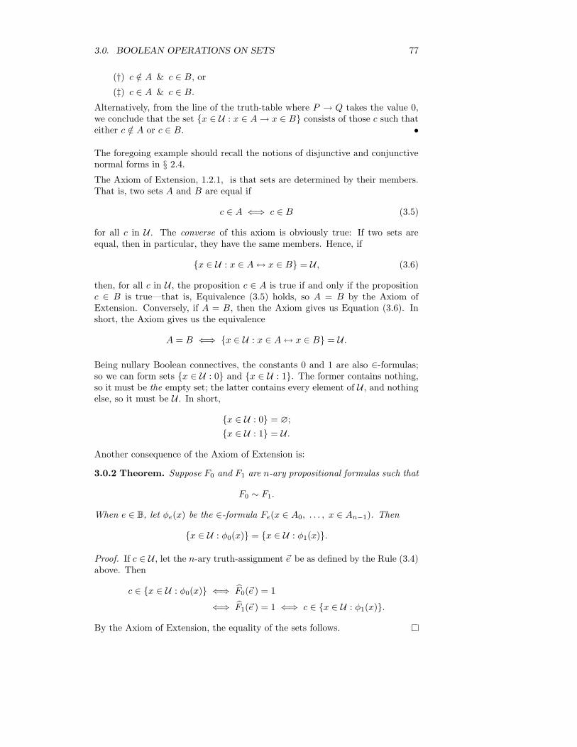
3.0. BOOLEAN OPERATIONS ON SETS 77
(†) c /∈ A & c ∈ B, or
(‡) c ∈ A & c ∈ B.
Alternatively, from the line of the truth-table where P → Q takes the value 0,we conclude that the set x ∈ U : x ∈ A→ x ∈ B consists of those c such thateither c /∈ A or c ∈ B. •
The foregoing example should recall the notions of disjunctive and conjunctivenormal forms in § 2.4.The Axiom of Extension, 1.2.1, is that sets are determined by their members.That is, two sets A and B are equal if
c ∈ A ⇐⇒ c ∈ B (3.5)
for all c in U . The converse of this axiom is obviously true: If two sets areequal, then in particular, they have the same members. Hence, if
x ∈ U : x ∈ A↔ x ∈ B = U , (3.6)
then, for all c in U , the proposition c ∈ A is true if and only if the propositionc ∈ B is true—that is, Equivalence (3.5) holds, so A = B by the Axiom ofExtension. Conversely, if A = B, then the Axiom gives us Equation (3.6). Inshort, the Axiom gives us the equivalence
A = B ⇐⇒ x ∈ U : x ∈ A↔ x ∈ B = U .
Being nullary Boolean connectives, the constants 0 and 1 are also ∈-formulas;so we can form sets x ∈ U : 0 and x ∈ U : 1. The former contains nothing,so it must be the empty set; the latter contains every element of U , and nothingelse, so it must be U . In short,
x ∈ U : 0 = ∅;
x ∈ U : 1 = U .
Another consequence of the Axiom of Extension is:
3.0.2 Theorem. Suppose F0 and F1 are n-ary propositional formulas such that
F0 ∼ F1.
When e ∈ B, let φe(x) be the ∈-formula Fe(x ∈ A0, . . . , x ∈ An−1). Then
x ∈ U : φ0(x) = x ∈ U : φ1(x).
Proof. If c ∈ U , let the n-ary truth-assignment ~e be as defined by the Rule (3.4)above. Then
c ∈ x ∈ U : φ0(x) ⇐⇒ F0(~e ) = 1
⇐⇒ F1(~e ) = 1 ⇐⇒ c ∈ x ∈ U : φ1(x).
By the Axiom of Extension, the equality of the sets follows.

78 CHAPTER 3. SETS AND RELATIONS
Example (3.0.1 continued). Because P → Q ∼ ¬P ∨Q, the two setsx ∈ U : x ∈ A→ x ∈ B and x ∈ U : x /∈ A ∨ x ∈ B are equal. •
We can say more. The following should be compared with Theorem 2.3.8:
3.0.3 Theorem (Replacement). Suppose F is a sub-formula of the n-ary for-mula G, so that G itself is H(P0, . . . , Pn−1, F ) for some formula H. Let
B = x ∈ U : F (x ∈ A0, . . . , x ∈ An−1).
Then the set x ∈ U : G(x ∈ A0, . . . , x ∈ An−1) is equal to
x ∈ U : H(x ∈ A0, . . . , x ∈ An−1, x ∈ B).
Proof. Exercise.
3.0.4 Corollary. For all ∈-formulas φ(x) and ψ(x),
x ∈ U : φ(x) ∧ ψ(x) = x ∈ U : φ(x) ∩ x ∈ U : ψ(x),x ∈ U : φ(x) ∨ ψ(x) = x ∈ U : φ(x) ∪ x ∈ U : ψ(x),x ∈ U : φ(x) = ψ(x) = x ∈ U : φ(x) M x ∈ U : ψ(x),
x ∈ U : ¬φ(x) = x ∈ U : φ(x)c.
Proof. Let A = x ∈ U : φ(x) and B = x ∈ U : ψ(x), and let H be thebinary formula P0 ∧ P1. Then
x ∈ U : φ(x) ∧ ψ(x)= x ∈ U : H(φ(x), ψ(x)) [by def’n of H]
= x ∈ U : H(x ∈ A, x ∈ B) [by Replacement]
= x ∈ U : x ∈ A ∧ x ∈ B [by def’n of H]
= A ∩B [by def’n of ∩]= x ∈ U : φ(x) ∩ x ∈ U : ψ(x) [by def’n of A and B].
The other identities are established likewise.
Example (3.0.1 continued again). We now have
x ∈ U : x ∈ A→ x ∈ B = x ∈ U : x /∈ A ∨ x ∈ B= x ∈ U : x /∈ A ∪ x ∈ U : x ∈ B= Ac ∪B,
and similarly, x ∈ U : x ∈ A → x ∈ B = (Ac ∩ Bc) ∪ (Ac ∩ B) ∪ (A ∩ B).Hence the equation
Ac ∪B = (Ac ∩Bc) ∪ (Ac ∩B) ∪ (A ∩B)
is an identity. •
3.0.5 Example. From the truth-table
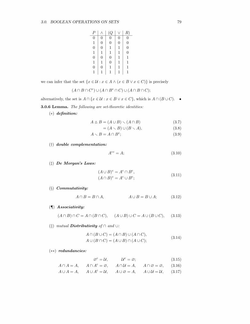
3.0. BOOLEAN OPERATIONS ON SETS 79
P ∧ (Q ∨ R)0 0 0 0 01 0 0 0 00 0 1 1 01 1 1 1 00 0 0 1 11 1 0 1 10 0 1 1 11 1 1 1 1
we can infer that the set x ∈ U : x ∈ A ∧ (x ∈ B ∨ x ∈ C) is precisely
(A ∩B ∩ Cc) ∪ (A ∩Bc ∩ C) ∪ (A ∩B ∩ C);
alternatively, the set is A ∩ x ∈ U : x ∈ B ∨ x ∈ C, which is A ∩ (B ∪ C). •3.0.6 Lemma. The following are set-theoretic identities:
(∗) definition:
A M B = (A ∪B) r (A ∩B) (3.7)
= (ArB) ∪ (B rA), (3.8)
ArB = A ∩Bc; (3.9)
(†) double complementation:
Acc = A; (3.10)
(‡) De Morgan’s Laws:
(A ∪B)c = Ac ∩Bc,
(A ∩B)c = Ac ∪Bc;(3.11)
(§) Commutativity:
A ∩B = B ∩A, A ∪B = B ∪A; (3.12)
(¶) Associativity:
(A ∩B) ∩ C = A ∩ (B ∩ C), (A ∪B) ∪ C = A ∪ (B ∪ C), (3.13)
(‖) mutual Distributivity of ∩ and ∪:
A ∩ (B ∪ C) = (A ∩B) ∪ (A ∩ C),A ∪ (B ∩ C) = (A ∪B) ∩ (A ∪ C); (3.14)
(∗∗) redundancies:
∅c = U , Uc = ∅; (3.15)
A ∩A = A, A ∩Ac = ∅, A ∩ U = A, A ∩∅ = ∅, (3.16)
A ∪A = A, A ∪Ac = U , A ∪∅ = A, A ∪ U = U , (3.17)
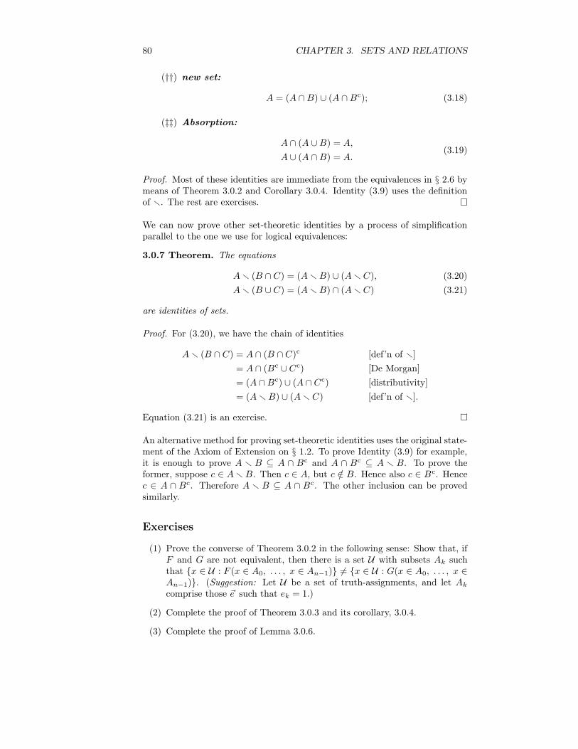
80 CHAPTER 3. SETS AND RELATIONS
(††) new set:
A = (A ∩B) ∪ (A ∩Bc); (3.18)
(‡‡) Absorption:
A ∩ (A ∪B) = A,
A ∪ (A ∩B) = A.(3.19)
Proof. Most of these identities are immediate from the equivalences in § 2.6 bymeans of Theorem 3.0.2 and Corollary 3.0.4. Identity (3.9) uses the definitionof r. The rest are exercises.
We can now prove other set-theoretic identities by a process of simplificationparallel to the one we use for logical equivalences:
3.0.7 Theorem. The equations
Ar (B ∩ C) = (ArB) ∪ (Ar C), (3.20)
Ar (B ∪ C) = (ArB) ∩ (Ar C) (3.21)
are identities of sets.
Proof. For (3.20), we have the chain of identities
Ar (B ∩ C) = A ∩ (B ∩ C)c [def’n of r]
= A ∩ (Bc ∪ Cc) [De Morgan]
= (A ∩Bc) ∪ (A ∩ Cc) [distributivity]
= (ArB) ∪ (Ar C) [def’n of r].
Equation (3.21) is an exercise.
An alternative method for proving set-theoretic identities uses the original state-ment of the Axiom of Extension on § 1.2. To prove Identity (3.9) for example,it is enough to prove A r B ⊆ A ∩ Bc and A ∩ Bc ⊆ A r B. To prove theformer, suppose c ∈ ArB. Then c ∈ A, but c /∈ B. Hence also c ∈ Bc. Hencec ∈ A ∩ Bc. Therefore A r B ⊆ A ∩ Bc. The other inclusion can be provedsimilarly.
Exercises
(1) Prove the converse of Theorem 3.0.2 in the following sense: Show that, ifF and G are not equivalent, then there is a set U with subsets Ak suchthat x ∈ U : F (x ∈ A0, . . . , x ∈ An−1) 6= x ∈ U : G(x ∈ A0, . . . , x ∈An−1). (Suggestion: Let U be a set of truth-assignments, and let Ak
comprise those ~e such that ek = 1.)
(2) Complete the proof of Theorem 3.0.3 and its corollary, 3.0.4.
(3) Complete the proof of Lemma 3.0.6.
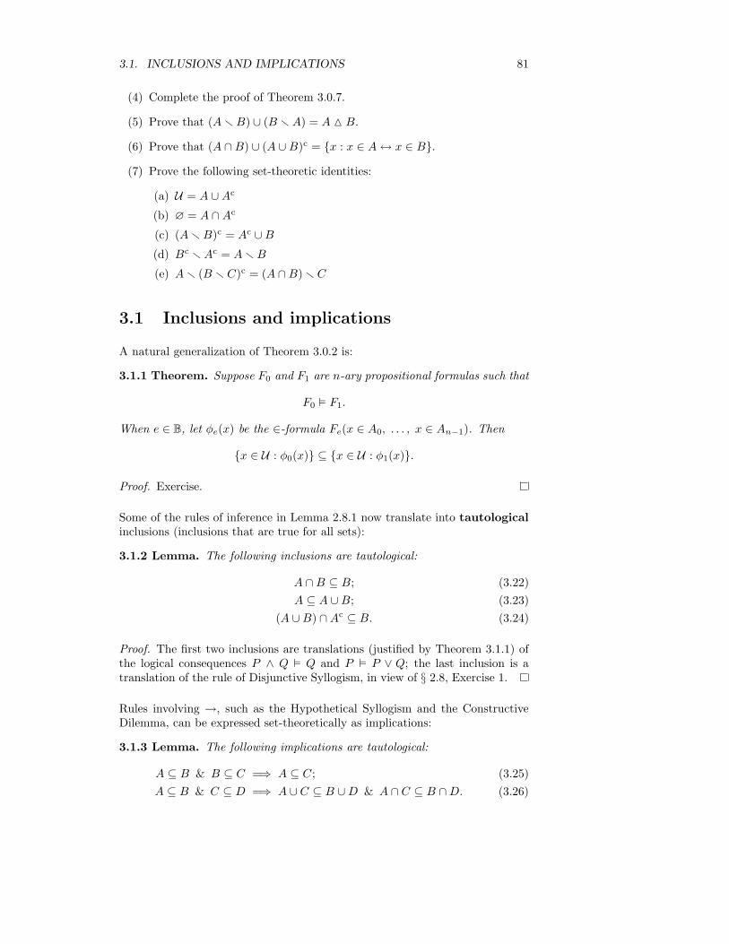
3.1. INCLUSIONS AND IMPLICATIONS 81
(4) Complete the proof of Theorem 3.0.7.
(5) Prove that (ArB) ∪ (B rA) = A M B.
(6) Prove that (A ∩B) ∪ (A ∪B)c = x : x ∈ A↔ x ∈ B.
(7) Prove the following set-theoretic identities:
(a) U = A ∪Ac
(b) ∅ = A ∩Ac
(c) (ArB)c = Ac ∪B(d) Bc rAc = ArB
(e) Ar (B r C)c = (A ∩B) r C
3.1 Inclusions and implications
A natural generalization of Theorem 3.0.2 is:
3.1.1 Theorem. Suppose F0 and F1 are n-ary propositional formulas such that
F0 ² F1.
When e ∈ B, let φe(x) be the ∈-formula Fe(x ∈ A0, . . . , x ∈ An−1). Then
x ∈ U : φ0(x) ⊆ x ∈ U : φ1(x).
Proof. Exercise.
Some of the rules of inference in Lemma 2.8.1 now translate into tautologicalinclusions (inclusions that are true for all sets):
3.1.2 Lemma. The following inclusions are tautological:
A ∩B ⊆ B; (3.22)
A ⊆ A ∪B; (3.23)
(A ∪B) ∩Ac ⊆ B. (3.24)
Proof. The first two inclusions are translations (justified by Theorem 3.1.1) ofthe logical consequences P ∧ Q ² Q and P ² P ∨ Q; the last inclusion is atranslation of the rule of Disjunctive Syllogism, in view of § 2.8, Exercise 1.
Rules involving →, such as the Hypothetical Syllogism and the ConstructiveDilemma, can be expressed set-theoretically as implications:
3.1.3 Lemma. The following implications are tautological:
A ⊆ B & B ⊆ C =⇒ A ⊆ C; (3.25)
A ⊆ B & C ⊆ D =⇒ A ∪ C ⊆ B ∪D & A ∩ C ⊆ B ∩D. (3.26)

82 CHAPTER 3. SETS AND RELATIONS
Proof. Suppose A ⊆ B and B ⊆ C and d ∈ A. Then d ∈ B, so d ∈ C. ThusA ⊆ C.
Suppose A ⊆ B and C ⊆ D. Say d ∈ A ∪ C. Then d ∈ A or d ∈ C. If d ∈ A,then d ∈ B, so d ∈ B ∪ D. The same conclusion follows similarly if d ∈ C.Therefore A ∪ C ⊆ B ∪D. The remaining inclusion is an exercise.
Implication (3.25) justifies abbreviating the proposition A ⊆ B & B ⊆ C by
A ⊆ B ⊆ C.
By Identities (3.16) and (3.17) above, Implication (3.26) has the special cases:
A ⊆ B & A ⊆ C =⇒ A ⊆ B ∩ C, (3.27)
A ⊆ B & C ⊆ B =⇒ A ∪ C ⊆ B. (3.28)
Their converses are a part of the following:
3.1.4 Lemma. The following are true for all sets:
(∗) A ⊆ B ∩ C =⇒ A ⊆ B;
(†) A ∪B ⊆ C =⇒ A ⊆ C;
(‡) A ∩B = ∅ & A ⊆ B =⇒ A = ∅;
(§) Ac ⊆ A ⇐⇒ Ac = ∅ ⇐⇒ A = U ;(¶) ArB = ∅ ⇐⇒ A ⊆ B.
Proof. Suppose A ⊆ B ∩ C. Since B ∩ C ⊆ B by Lemma 3.1.2, we get A ⊆ Bby Lemma 3.1.3. The remaining implications are exercises.
We are now equipped to prove some non-obvious claims:
3.1.5 Example. Suppose Ac ∪ (B M C) ⊆ A ∩Bc ∩ C. Then
A ∩ (B ∪ C) = (A ∪B) ∩ C. (3.29)
Indeed, to see this, note first
Ac ⊆ Ac ∪ (B M C) [by Lemma 3.1.2]
⊆ A ∩Bc ∩ C [by assumption]
⊆ A. [by Lemma 3.1.2]
Then Ac ⊆ A by Lemma 3.1.3, and therefore
A = U
by Lemma 3.1.4. By the same lemmas, and Lemma 3.0.6, our assumption nowgives us
(B r C) ∪ (C rB) = B M C ⊆ Bc ∩ C = B r C;
therefore C rB ⊆ B r C, that is,
C ∩Bc ⊆ B ∩ Cc.

3.1. INCLUSIONS AND IMPLICATIONS 83
Say a ∈ C ∩ Bc. Then a ∈ Bc. But also, a ∈ B ∩ Cc, so a ∈ B. Thusa ∈ Bc ∩B = ∅, which is absurd. So C ∩Bc must be empty, which means
B ⊆ C.
Finally then,A ∩ (B ∪ C) = B ∪ C = C = (A ∪B) ∩ C
since A = U = A ∪B. •
Where did this example come from? And, where did the proof come from?First, note that variations of the proof are possible: For example, part of theproof is showing
C ∩Bc ⊆ B ∩ Cc =⇒ C ∩Bc = ∅.
But if C ∩Bc ⊆ B ∩ Cc, then
C ∩Bc ⊆ (B ∩ Cc) ∩ (C ∩Bc) = B ∩ (Cc ∩ C) ∩Bc = ∅.
Thus there is no need to look at individual elements of C ∩Bc, as in the proofabove.
Whatever minor adjustments we make, the proof in Example 3.1.5 does notseem to follow a general pattern. Each step is justified, and the conclusion isas desired; so the proof is correct. But this observation does not tell us how tofind the proof.
There is an alternative proof that follows a general pattern; this proof alsosuggests how the proposition being proved was discovered. The key is the set-theoretic analogue of the disjunctive normal forms of § 2.4:Example (3.1.5 continued). We can analyze the given Boolean combinationsof A, B, and C as follows. First note that
Ac = (Ac ∩Bc) ∪ (Ac ∩B)
= (Ac ∩Bc ∩ Cc) ∪ (Ac ∩Bc ∩ C) ∪ (Ac ∩B ∩ Cc) ∪ (Ac ∩B ∩ C),while
B M C = (B ∩ Cc) ∪ (Bc ∩ C)= (Ac ∩B ∩ Cc) ∪ (A ∩B ∩ Cc) ∪ (Ac ∩Bc ∩ C) ∪ (A ∩Bc ∩ C).
Therefore
Ac ∪ (B M C) = (Ac ∩Bc ∩ Cc) ∪ (Ac ∩Bc ∩ C) ∪ (Ac ∩B ∩ Cc) ∪∪ (Ac ∩B ∩ C) ∪ (A ∩B ∩ Cc) ∪ (A ∩Bc ∩ C)
The six constituents of this union are disjoint, and the whole set Ac ∪ (B M C)is assumed to be a subset of its last constituent, A ∩Bc ∩C; therefore the firstfive constituents are empty. We aim to prove Equation (3.29). Analyzing thetwo members of this equation, we have
A ∩ (B ∪ C) = (A ∩B) ∪ (A ∩ C)= (A ∩B ∩ Cc) ∪ (A ∩B ∩ C) ∪ (A ∩Bc ∩ C),
(A ∪B) ∩ C = (A ∩ C) ∪ (B ∩ C)= (A ∩Bc ∩ C) ∪ (A ∩B ∩ C) ∪ (Ac ∩B ∩ C).
84 CHAPTER 3. SETS AND RELATIONS
Under the assumption, two constituents in each case are empty, and each mem-ber of Equation (3.29) is A ∩B ∩ C. •
Thus the alternative proof takes more writing, although it follows a generalprocedure that involves writing every set in question as a union of intersectionsof the sets A, B, and C and their complements.
Exercises
(1) Prove Theorem 3.1.1.
(2) Complete the proof of Lemma 3.1.3.
(3) Complete the proof of Lemma 3.1.4.
(4) Prove the following tautological inclusions:
(a) A ∩ (ArB)c ⊆ B
(b) Ar C ⊆ (ArB) ∪ (B r C)
(c) (ArB)c ∩ (B r C)c ⊆ (Ar C)c
(d) Ar C ⊆ (Ar (B r C)c) ∪ (ArB)
(e) A ⊆ Ar (B ∩Bc)
(f) (Ac rA)c ⊆ A
(g) Ac ⊆ Ac rA
(h) (A ∪B) r C ⊆ (Ar C) ∪ (B r C)
(i) Bc ⊆ (ArB) ∪ (Ac rB)
(j) ArB ⊆ Bc
(k) B rA ⊆ B
(5) Prove the following implications:
(a) U ⊆ B =⇒ U = B
(b) A ⊆ B & A ⊆ (B r C)c =⇒ A ⊆ C
(c) Ac ⊆ B ∩Bc =⇒ A = U(d) A ⊆ B & A ⊆ Bc =⇒ A = ∅
(e) Ac = U =⇒ A ⊆ B
(f) A ⊆ B =⇒ A ∩ C ⊆ B ∩ C(6) Prove the following equivalences:
(a) A ⊆ B ⇐⇒ Ac ∪B = U(b) A 6⊆ B ⇐⇒ A ∩Bc 6= ∅
(c) A ⊆ B ⇐⇒ Bc ⊆ Ac
(d) A ⊆ (B r C)c ⇐⇒ A ∩B ⊆ C
(7) Simplify (Ac ∩Bc ∩Cc)∪ (Ac ∩Bc ∩C)∪ (Ac ∩B ∩Cc)∪ (Ac ∩B ∩C)∪(A ∩B ∩ Cc) ∪ (A ∩Bc ∩ C) to the form Ac ∪ (B M C).
(8) Compose an example like 3.1.5.

3.2. CARTESIAN PRODUCTS, AND RELATIONS 85
A
B A×B
Figure 3.2: Cartesian product
3.2 Cartesian products, and relations
Suppose φ(x) is an ∈-formula as in § 3.0, Line (3.2). We can say that thisformula defines, in U , the set x ∈ U : φ(x); and this set can be calledthe interpretation of φ(x) in U . The interpretation of φ(x) may change if Uchanges. For example, the interpretation of x /∈ A in U is U rA, which dependson U . However, as long as U includes A, the interpretation of x ∈ A in U doesnot change: it is just A.
We now allow variables besides x, and we ask, for example, whether the binary∈-formula
x ∈ A ∧ y ∈ Bdefines a set. It does define a set, which is denoted
A×B
and called the Cartesian product of A and B. This set A×B can be depictedas in Figure 3.2. If a ∈ A and b ∈ B, then there will be an element of A × B,denoted
(a, b)
and called an ordered pair. Such objects will have the property that
(a, b) = (a′, b′) ⇐⇒ a = a′ & b = b′; (3.30)
consequently,(a, b) ∈ A×B ⇐⇒ a ∈ A & b ∈ B.
But what is an ordered pair?
So far (in this chapter), all of our sets have been Boolean combinations of givensets. A completely different way of producing sets is usually taken as an axiom:
3.2.1 Axiom (Pairing). For any two objects (possibly not distinct), there is aset whose elements are precisely those objects. That is, for all a and b, the set
a, b
exists.
86 CHAPTER 3. SETS AND RELATIONS
This axiom involves an existential statement. In particular, the axiom can bewritten formally as
∀x ∀y ∃z ∀w (w ∈ z ↔ w = x ∨ w = y).
When one formalizes set-theory in this way, one usually understands the vari-ables (here x, y, z, and w) to range only over sets. We are not being so restrictive,for now.
If a = b, then the set a, b is just
a,
which contains nothing but a and can be called a singleton. (We saw thisnotion in § 1.2.) If a 6= b, then a, b is an (unordered) pair or a doubleton.
3.2.2 Lemma. a, a, b = c, c, d ⇐⇒ a = c & b = d.
Proof. Exercise.
Now we can define ordered pairs so as to have the desired Property (3.30): bydefinition,
(a, b) = a, a, b.Note well that we make this definition solely so that ordered pairs will haveProperty (3.30). It is true but unimportant2 that a ∈ (a, b)—except that, inthe usual treatment of set-theory, one still needs the precise definition of (a, b)to justify axiomatically the existence of the set A×B. I shall discuss this pointlater. Meanwhile, we can write
A×B = (x, y) ∈ U × U : x ∈ A ∧ y ∈ B.
Suppose now F is a 2n-ary propositional formula. Then we have the binary∈-formula
F (x ∈ A0, . . . , x ∈ An−1, y ∈ A0, . . . , y ∈ An−1). (3.31)
Call this φ(x, y). Its interpretation in U is a subset of U × U , namely
(x, y) ∈ U × U : φ(x, y), (3.32)
which consists precisely of those (c, d) in U × U such that
F (~e , ~f ) = 1,
where ~e and ~f are the n-ary truth assignments such that
ek = 1 ⇐⇒ c ∈ Ak,
fk = 1 ⇐⇒ d ∈ Ak
for each k in 0, . . . , n− 1. As special cases, we have
(x, y) ∈ U × U : x ∈ A = A× U ;(x, y) ∈ U × U : y ∈ B = U ×B.
2Some discussion of this point is in [16, § 6].
3.2. CARTESIAN PRODUCTS, AND RELATIONS 87
These sets are also the interpretations in U × U of (x, y) ∈ A × U and (x, y) ∈U × B respectively. Hence, for example, the formulas x ∈ A and (x, y) ∈A × U are interchangeable or, as we may say, equivalent as binary formulas.In Line (3.32), we can now replace φ(x, y) with the formula
F ((x, y) ∈ A0 × U , . . . , (x, y) ∈ An−1 × U ,(x, y) ∈ U ×A0, . . . , (x, y) ∈ U ×An−1), (3.33)
without changing the set.
Since we have a new operation on sets, we may wonder how it interacts withthe ones that we already have. Let use first establish the notational conventionthat × has priority over ∩, ∪, M, and r, but not over c, so that, for example,
A×B ∩ C = (A×B) ∩ C;A×Bc = A× (Bc).
Then we have:
3.2.3 Theorem. The following are set-theoretic identities:
A× (B ∩ C) = A×B ∩A× C, (A ∩B)× C = A× C ∩B × C,A× (B ∪ C) = A×B ∪A× C, (A ∪B)× C = A× C ∪B × C,
U ×Ac = (U ×A)c, Ac × U = (A× U)c.
Proof. We prove the first identity in two ways; the rest are exercises.
Suppose (a, b) ∈ A × (B ∩ C). Then a ∈ A, and b ∈ B ∩ C. Hence alsob ∈ B and b ∈ C. Therefore (a, b) ∈ A × B and (a, b) ∈ A × C. Consequently(a, b) ∈ (A×B)∩ (A×C). Thus A× (B ∩C) ⊆ (A×B)∩ (A×C). The reverseinclusion is an exercise.
Alternatively, we have
A× (B ∩ C) = (x, y) ∈ U × U : x ∈ A ∧ y ∈ B ∩ C= (x, y) ∈ U × U : x ∈ A ∧ y ∈ B ∧ y ∈ C= (x, y) ∈ U × U : (x ∈ A ∧ y ∈ B) ∧ (x ∈ A ∧ y ∈ C)= (x, y) ∈ U × U : (x, y) ∈ A×B ∧ (x, y) ∈ A× C,
which is (A × B) ∩ (A × C) by definition of intersection. To save writing, wemight just note that A×(B∩C) is the interpretation of the following equivalentformulas:
x ∈ A ∧ y ∈ B ∩ C, x ∈ A ∧ y ∈ B ∧ y ∈ C,(x ∈ A ∧ y ∈ B) ∧ (x ∈ A ∧ y ∈ C), (x, y) ∈ A×B ∧ (x, y) ∈ A× C
—while the last formula defines (A×B) ∩ (A× C).
The identity for A×Bc is not so neat: see Exercise 3. Part of the last theoremcan be generalized:

88 CHAPTER 3. SETS AND RELATIONS
-
6
c c c c cc c c cc c cc ccs s s s
s s ss ss
Figure 3.3: The less-than relation on Z
3.2.4 Theorem. The equation
A×B ∩ C ×D = (A ∩ C)× (B ∩D)
is an identity.
Proof. A×B ∩ C ×D is the interpretation of
x ∈ A ∧ y ∈ B ∧ x ∈ C ∧ y ∈ D,
which is equivalent to
x ∈ A ∧ x ∈ C ∧ y ∈ B ∧ y ∈ D,
which is the interpretation of (A ∩ C)× (B ∩D).
For A×B ∪ C ×D and (A×B)c, see Exercise 5.
We have observed that the formulas on Lines (3.31) and (3.33) are equivalent.This suggests a further generalization: If (R0, . . . , Rn−1) is a list of n subsets ofU×U , and G is an n-ary propositional formula, then we have a binary ∈-formula
G((x, y) ∈ R0, . . . , (x, y) ∈ Rn−1).
We have binary analogues of Theorems 3.0.2 and 3.1.1 (which I shall not writedown).
A subset of U × U is a binary relation on U . If R ⊆ U × U , and (a, b) ∈ R,then we may also write
a R b.
Then R = (x, y) ∈ U × U : x R y.
3.2.5 Example. The less-than relation on Z (named in § 1.3) is the set
(x, y) ∈ Z× Z : x < y,
which can be depicted as in Figure 3.2. •
There are two generalizations:

3.2. CARTESIAN PRODUCTS, AND RELATIONS 89
(∗) If R ⊆ A×B, then R is a relation from A to B; also, A is the domainof R, and B is the co-domain.
(†) There are n-ary relations for every n in N.
The first of these will be taken up in the next section. On the latter point, notethat we can form an n-ary ∈-formula
x0 ∈ A0 ∧ . . . ∧ xn−1 ∈ An−1;
its interpretation in U can be denoted
A0 × · · · ×An−1.
This is a subset of U × · · · × U︸ ︷︷ ︸n
, which we can also denote
Un.
The elements of Un are just the (ordered) n-tuples
(c0, . . . , cn−1) or ~c
where each ck is in U . Such an n-tuple is just what we have called a list of nelements of U . In particular, an n-ary truth-assignment is an element of Bn.
Instead of A × A, we can write A2. We can let A1 be A itself. We can defineA3 to be A2 × A; define A4 to be A3 × A; and so on. By our precise definitionthen,
(a0, . . . , an) = ((a0, . . . , an−1), an) = (a0, . . . , an−1), (a0, . . . , an−1), an,
but this is not important; we could also use the definition
(a0, . . . , an−1) = a0, a0, a1, . . . , a0, a1, . . . , an−1
for example. (See also § 3.6.) In any case, we should understand
(a0, . . . , an−1) =
a0, if n = 1;
∅, if n = 0;
that is, (a) is just a, and ( ) is ∅. Then A1 = A as we said; also, A0 = ∅, whichis 1 in the von-Neumann definition of the natural numbers in § 1.2. Finally, if ~ais the n-tuple (a0, . . . , an−1), and ~b is the m-tuple (b0, . . . , bm−1), then we treat
the ordered pair (~a ,~b ) as the ordered (n+m)-tuple (a0, . . . , an−1, b0, . . . , bm−1).Then we have
Am ×An = Am+n
for all m and n in ω. (We do not have a meaning for An if n is a negativeinteger.)
An n-ary relation on U is a subset of Un. In particular, a singulary relationon U is just a subset of U . A nullary relation on U is a subset of U 0; which is∅; so a nullary relation is either ∅ or ∅. In the von-Neumann definition,these sets are 0 and 1 respectively; so a nullary relation is just a truth-value.
An n-ary predicate is a name for an n-ary relation. An n-ary relation is thena possible interpretation of an n-ary predicate.

90 CHAPTER 3. SETS AND RELATIONS
Exercises
(1) Prove Lemma 3.2.2.
(2) Complete the proof of Theorem 3.2.3.
(3) Prove the identity A×Bc = A× U r U ×B.
(4) Prove the identities:
(a) (A M B)× C = A× C M B × C;(b) (ArB)× C = A× C rB × C.
(5) Prove the identities:
(a) A×B ∪ C ×D = ((A ∪ C)× (B ∪D) rAc ×Dc) r Cc ×Bc;
(b) (A×B)c = Ac × U ∪ U ×Bc.
3.3 Functions
A relation R from a set A to a set B is a function from A to B if it has twoproperties:
(∗) For every a in A there is some b in B such that (a, b) ∈ R.(†) If R contains both (a, b) and (a, c), then b = c.
One might abbreviate these properties as follows:
(∗) (∀x ∈ A) (∃y ∈ B) x R y.
(†) (∀x ∈ A) (∀y ∈ B) (∀z ∈ B) (x R y & x R z =⇒ y = z).
Alternatively, R is a function if it has the property:
(∗) For every a in A, there is a unique b in B such that a R b.
Unique existence—existence of exactly one—is sometimes abbreviated by thequantifier
∃!.Then the last property can be abbreviated:
(∗) (∀x ∈ A) (∃! y ∈ B) a R b.
Often a function is denoted by a letter like f ; then, instead of writing (a, b) ∈ f ,or a f b, one writes
f(a) = b.
Suppose f is a function from A to B. This can be indicated by
f : A −→ B or Af−→ B.
In accordance with the definitions in the previous section, A is then the domainof f , and B is the co-domain of f . Also, f is a function on A, and f is afunction from A to B. Functions are sometimes called maps; in the presentcase, f can be said to map A into B.
3.3. FUNCTIONS 91
Considered as a string of symbols, f(x) is a term. Then the function f mightbe given by the notation
x 7−→ f(x),
and we might say that f takes or sends x to f(x). As we shall see presently,the term f(x) might be replaced with another term that does not contain aspecific name for f itself.
An n-ary operation on a set A is a function from An to A. Then there isat least one singulary operation on A, namely the identity on A: this is thefunction
x 7−→ x
on A, which can be denotedidA.
More generally, if k < n, then there is an n-ary operation
(x0, . . . , xn−1) 7−→ xk
on A. (This operation is idA if n = 1 and k = 0.) But there are all sorts ofoperations besides these:
3.3.1 Examples.
(∗) In §1.2, the successor of a number n in N is denoted n+ or n+ 1. Thismeans there is a function x 7→ x+ from N to itself; this is a singularyoperation on N.
(†) The operations + and · named in § 1.3 are binary operations on Z andcan be denoted (x, y) 7→ x+ y and (x, y) 7→ xy respectively.
(‡) Hence any arithmetic term t in an n-tuple (x0, . . . , xn) of variablesdetermines the n-ary operation ~x 7→ t on Z.
(§) The fundamental theorem of calculus is that if f is a continuous func-tion on R, and a ∈ R, then the function x 7→
∫ xaf is a primitive for f
(that is, a function whose derivative is f). •
Several refinements of the notion of a function are useful. Suppose again thatf : A→ B. Then f is:
(∗) surjective or onto, if every element of B is f(a) for at least one a in A;
(†) injective or one-to-one, if every element of B is f(a) for at most one ain A;
(‡) bijective, if it is one-to-one and onto (injective and surjective).
A surjective function is a surjection; an injective function is an injection; abijective function is a bijection. An injection is also called an embedding; abijection is also called a one-to-one correspondence. More symbolically, fis:
(∗) surjective, if (∀y ∈ B) (∃x ∈ A) f(x) = y;
(†) injective, if (∀x ∈ A) (∀y ∈ A) (f(x) = f(y) =⇒ x = y).
3.3.2 Examples.

92 CHAPTER 3. SETS AND RELATIONS
(∗) idA is a bijection.
(†) The squaring function x 7→ x2 is injective on N, but not on Z; as afunction from C to C, it is surjective, but not as a function from R to R.
(‡) The tangent-function x 7→ tanx from R to R is surjective, but notinjective.
(§) The cubing function x 7→ x3 from R to R is bijective. •
Again suppose f : A→ B. The range of f is the set
y ∈ B : (∃x ∈ A) f(x) = y;
this is a subset of the co-domain of f , and can be denoted
f(x) : x ∈ A,
or more simplyf(A).
Since this notation suggests—usually wrongly—that A is actually an elementof the domain of f , I shall also use the notation
f [A].
A function is surjective if and only if its range is equal to its co-domain.
3.3.3 Examples.
(∗) The co-domain of x 7→ sinx is usually considered to be R, although therange of the function is the interval [−1, 1].
(†) The function x 7→ 1 + x2, as a function on R, has range [1,∞). •
Suppose also g : B → C. The composition of f and g is
(x, z) ∈ A× C : g(f(x)) = z;
This can be denotedg f,
which can be read as g composed with f . Showing that g f is a functionis Exercise 1 below; it is Exercise 2 to show that the composition of injectivefunctions is injective, and the composition of surjective functions is surjective.
Many of the foregoing ideas are connected by the following:
3.3.4 Theorem. Suppose A 6= ∅ and f : A→ B.
(0) The function f is injective if and only if gf = idA for some function gfrom B to A.
(1) The function f is surjective if and only if fg = idB for some function gfrom B to A.
(2) The function f is bijective if and only if g f = idA and f g = idBfor some function g from B to A.

3.3. FUNCTIONS 93
Proof. (0) Suppose f is injective. Then for every b in f [A], there is exactly onea in A such that f(a) = b. This means that the set (f(x), x) : x ∈ A is afunction from f [A] to A. Since A 6= ∅, there is some c in A; then y 7→ c is afunction from B r f [A] to A. The union of these two functions, as sets, is afunction g from B to A, and g(f(a)) = a for all a in A, so g f = idA.
Suppose conversely that g f = idA. If f(a) = f(a′), then g(f(a)) = g(f(a′)),that is, idA(a) = idA(a
′), which means a = a′. Thus f is injective.
(1) Suppose f is surjective. Then for every b in B, there is at least one a in Asuch that f(a) = b. Now we have to do something sneaky: We pick one sucha, and define g(b) = a. We do this for all b in B, and this gives us g as desired.(That such picking can be done once for all is perhaps not obvious, but it is aconsequence of the set-theoretic Axiom of Choice.)
The converse, and (2), are left as an exercise.
3.3.5 Theorem. Suppose f : A → B and is bijective. Then there is exactlyone function g from B to A such that g f = idA and f g = idB.
Proof. By the last theorem, there is at least one such function. Suppose g0 andg1 are such functions, and b ∈ B. Then b = f(a) for some a in A, since f issurjective. Hence
g0(b) = g0(f(a)) = g0 f(a) = idA(a) = g1 f(a) = g1(f(a)) = g1(b).
Thus g0 = g1.
The unique function g in the theorem is the inverse of f and can be denoted
f−1.
A bijection can also be called an invertible function.
In general, if f : A→ B and C ⊆ A, then f ∩ (C × B) is a function from C toB; this can be denoted by
f ¹ C;
it is the restriction of f to C, and its range is f [C].
Exercises
(1) Show that the composition of two functions is a function.
(2) Show that the composition if injective functions is injective; of surjective,surjective.
(3) Complete the proof of Theorem 3.3.4.
(4) Suppose f and g are functions from A to B. For each of the followingrelations,
• prove whether it is always a function; and
• prove whether it is always not a function:

94 CHAPTER 3. SETS AND RELATIONS
(a) f ∪ g;(b) f ∩ g;(c) f g−1;
(d) f−1 g.
(5) Let f : A→ B and g : B → C.
(a) Supposing g and f are invertible, write (g f)−1 as a composition ofinverses (rather than an inverse of compositions).
(b) If g f is injective, does it follow that f is injective?—that g isinjective?
(c) Same question, with surjective for injective.
(d) Same question, with bijective for surjective.
3.4 Deeper into functions
Induced functions
If f : A → B and C ⊆ A, then we have defined f [C] as a subset of B. Thissuggests that we have a function X 7→ f [X]; but what are its domain andco-domain?
3.4.1 Axiom (Power-set). If A is a set, then the class of subsets of A is a set.
The set of subsets of A can be denoted
P(A);
it is called the power-set of A.
3.4.2 Examples.
(∗) P(∅) = ∅, that is, P(0) = 1 in the definition of von Neumann;
(†) P(∅) = ∅, ∅, that is, P(1) = 2.
(‡) ∅ ∈ P(A) and A ∈ P(A) for all sets A.
Hence, if f : A → B, then the function X 7→ f [X] has the domain P(A) andthe co-domain P(B).
3.4.3 Lemma. Suppose f : A→ B. Then
X ⊆ Y =⇒ f [X] ⊆ f [Y ]
for all subsets X and Y of A.
Proof. Suppose x ∈ f [X]. Then x = f(u) for some u in X. But X ⊆ Y , sou ∈ Y , and hence f(u) ∈ f [Y ], that is, x ∈ f [Y ].

3.4. DEEPER INTO FUNCTIONS 95
3.4.4 Theorem. Suppose f : A→ B. Then
f [X ∪ Y ] = f [X] ∪ f [Y ], (3.34)
f [X ∩ Y ] ⊆ f [X] ∩ f [Y ] (3.35)
for all subsets X and Y of A.
Proof. We have that f [X] and f [Y ] are subsets of f [X ∪ Y ] by the last lemma.Hence
f [X] ∪ f [Y ] ⊆ f [X ∪ Y ]
by (3.28). For the reverse inclusion, suppose x ∈ f [X ∪ Y ]. Then x = f(u) forsome u in X ∪ Y . Either u ∈ X or u ∈ Y , hence, either x ∈ f [X] or x ∈ f [Y ].In either case, x ∈ f [X] ∪ f [Y ]. This proves (3.34).
For (3.35), note that if f [X ∩ Y ] is a subset of both f [X] and f [Y ], by the lastlemma; we are now done, by (3.27).
3.4.5 Example. The inclusion (3.35) can be strict. For example, if f is(0, 0), (1, 0) and X = 0 and Y = 1, then X ∩ Y = ∅, but f [X] ∩ f [Y ] =0. •3.4.6 Theorem. Suppose f : A→ B.
(1) The following are equivalent:
(∗) f is injective.
(†) f [X ∩ Y ] = f [X] ∩ f [Y ] for all subsets X and Y of A.
(2) If f is injective, then
f [Xc] ⊆ (f [X])c,
f [X r Y ] ⊆ f [X] r f [Y ]
for all subsets X and Y of A.
(3) The following are equivalent:
(∗) f is bijective.
(†) f [Xc] = (f [X])c for all subsets X of A.
Proof. Exercise.
If f : A→ B, and C ⊆ B, then A has the subset
x ∈ A : f(x) ∈ C,
which can be denotedf−1[C].
Thus we have a functionY 7−→ f−1[Y ]
with domain P(B) and co-domain P(A). Note well that this function exists,whether f is invertible or not. The function Y 7→ f−1[Y ] behaves more nicelythan X 7→ f [X] with respect to the Boolean operations:
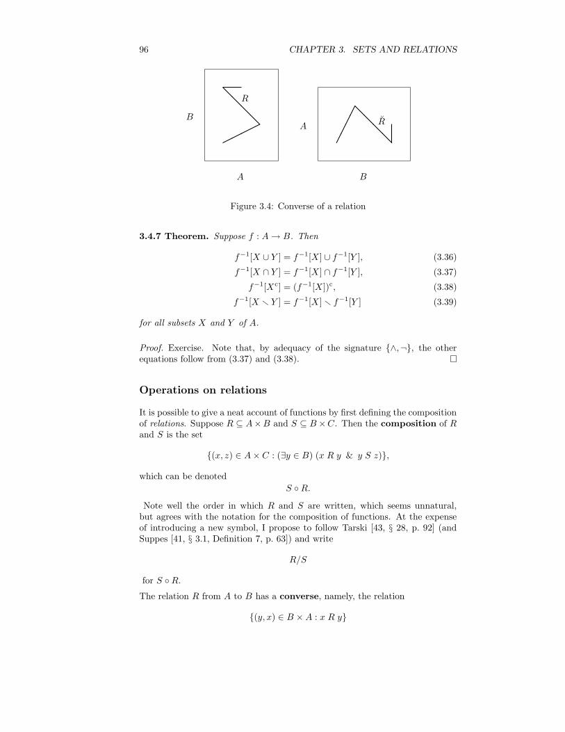
96 CHAPTER 3. SETS AND RELATIONS
©©©©
@@@@B
A
R
¢¢¢¢
@@
@@
B
AR
Figure 3.4: Converse of a relation
3.4.7 Theorem. Suppose f : A→ B. Then
f−1[X ∪ Y ] = f−1[X] ∪ f−1[Y ], (3.36)
f−1[X ∩ Y ] = f−1[X] ∩ f−1[Y ], (3.37)
f−1[Xc] = (f−1[X])c, (3.38)
f−1[X r Y ] = f−1[X] r f−1[Y ] (3.39)
for all subsets X and Y of A.
Proof. Exercise. Note that, by adequacy of the signature ∧,¬, the otherequations follow from (3.37) and (3.38).
Operations on relations
It is possible to give a neat account of functions by first defining the compositionof relations. Suppose R ⊆ A×B and S ⊆ B×C. Then the composition of Rand S is the set
(x, z) ∈ A× C : (∃y ∈ B) (x R y & y S z),
which can be denoted
S R.Note well the order in which R and S are written, which seems unnatural,but agrees with the notation for the composition of functions. At the expenseof introducing a new symbol, I propose to follow Tarski [43, § 28, p. 92] (andSuppes [41, § 3.1, Definition 7, p. 63]) and write
R/S
for S R.The relation R from A to B has a converse, namely, the relation
(y, x) ∈ B ×A : x R y

3.4. DEEPER INTO FUNCTIONS 97
¡¡¡¡¡¡¡¡¡¡
A
A
∆A
Figure 3.5: Diagonal on a set
from B to A; it can be denoted
R.
(See Figure 3.4.) This is sometimes denoted R−1, but this notation can bemisleading.
Finally, the binary relation of equality on A is just the set
(x, y) ∈ A×A : x = y.
We can also call this the diagonal on A, and give it the symbol
∆A.
(The delta stands for diagonal; see Figure 3.5.)
We can now make the following definitions: R is
(∗) full, if ∆A ⊆ R/R;
(†) functional, if R/R ⊆ ∆B .
3.4.8 Theorem. Let R ⊆ A × B. Then R is a function from A to B if andonly if R is full and functional (as a relation from A to B).
Proof. Exercise.
We have alternative characterizations for notions in § 3.3:
3.4.9 Theorem. Suppose f : A→ B.
(∗) f is surjective if and only if ∆B ⊆ f/f ;
(†) f is injective if and only if f/f ⊆ ∆A;
(‡) f is bijective if and only if f/f = ∆B and f/f = ∆A.
Proof. Exercise.
98 CHAPTER 3. SETS AND RELATIONS
Exercises
(1) Prove Theorem 3.4.6.
(2) Prove Theorem 3.4.7.
(3) Prove Theorem 3.4.8.
(4) Prove Theorem 3.4.9.
3.5 First-order logic
First-order logic provides a formal way to talk about particular operations andrelations. It allows for a precise definition of the context, mentioned in § 1.1,in which a mathematical proposition is true or false. First-order logic is a largesubject; this section will be only a cursory treatment. However, we have alreadymentioned the ingredients of first-order logic, in an informal way at least. Asignature L for a first-order logic consists of constants, function-symbols, andpredicates. A structure in the signature L is a non-empty set A along with afunction that takes:
(∗) each constant of L to an element of A;
(†) each function-symbol of L to an operation on A;
(‡) each predicate of L to a relation on A.
Thus the elements of L symbolize elements of A and operations and relationson A. More elements and operations are symbolized by terms, which are stringsmade of constants, function-symbols, and variables. More relations are symbol-ized by formulas. The simplest formulas are the atomic3 formulas, which consistof terms joined by the sign of equality or by a predicate. Atomic formulas can bepreceded by quantifiers (with variables) or combined by means of Boolean con-nectives; formulas in general are obtained in this way. New constants standingfor particular elements of A can be used as parameters in terms and formulas.
3.5.1 Example. The set Z of integers can be understood as a structure in thesignature +,−, ·, 0, 1, < (see § 1.3 (1.10)); a term in this signature (with pa-rameters from Z as desired) is an arithmetic term as defined in § 1.3. (However,the general definition of terms given below will use Polish notation as in § 2.1.)Diophantine equations and arithmetic inequalities are the atomic formulas inthis signature. •
The terminology of first-order logic is a means to give a precise but generalaccount of some ideas that one encounters in high-school mathematics.
Structures
By formal definition, a structure is an ordered pair (A, I)—which can also bereferred to as A—where:
3From the Greek Łtomoc uncuttable, not compound, from tìmoc a slice.
3.5. FIRST-ORDER LOGIC 99
(∗) A is a non-empty set, which is called the universe of the structure;
(†) I is a function, written also
s 7−→ sA,
whose domain L is called the signature of the structure;
(‡) sA is either an element of A or an n-ary operation or relation on A forsome positive n, for each s in L.
If L = s0, s1, . . . , then A can be written as
(A, s0A, s1
A, . . . ),
or just as (A, s0, s1, . . . ) unless ambiguity would result (that is, unless somestructure different from A has the same universe and the same signature).
3.5.2 Examples. The following are structures:
(1) (N,+, 0) (see § 1.2), or more briefly N;
(2) the power-set structure on a non-empty set Ω, namely
(P(Ω),∩,∪, c,∅,Ω,⊆);
(3) the truth-structure4
(B,∧,∨,¬, 0, 1,²),
where ² is the binary relation (0, 0), (0, 1), (1, 1) on B. •
The last two examples are the same if the elements of B are von-Neumannnatural numbers and Ω is the von-Neumann natural number 1. Propositionallogic studies the truth-structure. The area of mathematics and logic calledmodel-theory studies all structures.
When I is as above in the structure (A, I), and s is an element of L, then:(∗) sA is called the interpretation in A of s;
(†) s is called a symbol for sA.
So s is one of the following, according to its interpretation:
(∗) a constant;
(†) an n-ary function-symbol for some positive n in ω;
(‡) an n-ary predicate (or relation-symbol) for some positive n in ω.
Since nullary operations on A can be considered as elements of A, a constantcan be considered as a nullary function-symbol.
Here are some observations about the definition of structure:
4The name truth-structure is my invention.

100 CHAPTER 3. SETS AND RELATIONS
(∗) I am following the old convention5 of denoting the universe of a structureby a Roman letter, and the structure itself by the corresponding Fraktur orGothic letter. One might not bother to make a typographical distinctionbetween a structure and its universe. Indeed, as suggested in the examples,the distinction is not easy to make with standard structures like B or Z(which are commonly denoted by letters in a so-called blackboard-boldfont).
(†) Similarly, it is not always easy or convenient to distinguish in writingbetween a symbol and its interpretation.
(‡) In a structure (A, I), the interpretation-function I could be consideredto carry, within itself, the universe A. In any case, A and I work togetherto provide interpretations of the symbols in L as elements of, or operationsor relations on, a certain set, namely A itself. That’s all a structure is:something that provides a mathematical interpretation for certain sym-bols. What makes model-theory interesting is that the same symbols canhave different interpretions. Here begins the distinction between syntax(formal symbolism) and semantics (mathematical meaning).
Terms and formulas
The terms of a first-order signature L are conveniently written in Polish nota-tion (see § 2.1). First, we introduce a list
x0, x1, x2, . . .
of variables (that is, of individual variables: variables standing for individualelements of a universe). Then, by definition,
(∗) all variables are terms of L;(†) all constants of L are terms of L;(‡) if f is an n-ary function-symbol in L, and (t0, . . . , tn−1) is a list of n terms
of L, thenft0 · · · tn−1
is a term of L; if f is binary, then ft0t1 may also be written
(t0 f t1).
Finally, singulary function-symbols are sometimes written as superscriptson their arguments: examples include n+ in § 1.2, Line (1.5), and Ac in§ 1.9, Line (1.23).
The atomic formulas are defined similarly:
5Used for example in [6]. Recent writers (as in [27] or [35]) use ‘calligraphic’ letters, notFraktur:
For a structure with universe: A B C . . . M N . . .
I write: A B C . . . M N . . .
Others may write: A B C . . . M N . . .Another option (taken in [20]) is to use an ordinary letter like A for a structure, and thendom(A) for its universe. (Here dom stands for domain.)
3.5. FIRST-ORDER LOGIC 101
(∗) if t0 and t1 are terms of L, then the equation
t0 = t1
is an atomic formula of L;(†) if R is an n-ary predicate of L, and (t0, . . . , tn−1) is a list of n terms of L,
then the stringRt0 · · · tn−1
is a term of L; if R is binary, then Rt0t1 may also be written
t0 R t1.
Finally, formulas in general can be defined:
(∗) atomic formulas of L are formulas of L;(†) if φ is a formula of L, then so is ¬φ;(‡) if φ and χ are formulas of L, then (φ ∧ χ) is a formula of L;(§) if φ is a formula of L, and x is an individual variable, then ∃x φ is a
formula of L.These are the first-order formulas in the signature L; they constitute thefirst-order logic in that signature. We can use other connectives in additionto, or instead of, ¬ and ∧. One will generally want to use an adequate signaturefor propositional logic, like ¬,∧. Once the criterion of adequacy is met, thenusing fewer symbols makes the ensuing definitions and proofs easier to writedown.
We can also use the quantifier ∀; but formulas using ∀ can be rewritten with ∃alone by means of (1.24) and (1.25) in § 1.9.It is standard to write a formula ¬(t0 = t1) as t0 6= t1.
Interpretations of formulas
A term t can be called n-ary if the set of its variables is a subset of xk : k < n;then t is interpreted in an L-structure A as an n-ary operation tA on A. Thepossibility that n = 0 is allowed; in that case, t is nullary or constant, and itsinterpretation in A is just an element of A. The precise definition is what oneshould expect:
(∗) if k < n, then the variable xk is an n-ary term, and as such is interpretedin A as the n-ary operation ~x 7→ xk on A (here necessarily n > 0);
(†) every constant c is an n-ary term, interpreted in A as the constant n-aryoperation ~x 7→ cA on A (or just as cA, if n = 0);
(‡) if (t0, . . . , tk−1) is a list of n-ary terms, and f is a k-ary function-symbol,then the term ft0 · · · fk−1 is n-ary and, as such, is interpreted in A as then-ary operation
~x 7−→ fA(t0A(~x ), . . . , tk−1
A(~x ))
on A (or as fA(t0A, . . . , tk−1
A), if n = 0).

102 CHAPTER 3. SETS AND RELATIONS
3.5.3 Example. In Z, the two ternary terms (x0 · (x1 + x2)) and ((x0 · x1) +(x0 ·x2)) have the same interpretation, namely the ternary operation (x, y, z) 7→x(y + z) on Z. We could also write this operation more precisely as (x, y, z) 7→x ·Z (y +Z z). (See § 1.3 (1.7).) •
Interpretations of formulas take longer to define precisely, but the idea is that ¬,∧, and ∃ symbolize complementation, intersection, and projection respectively.An atomic formula φ can be called n-ary if the set of its variables is a subset ofxi : i < n. Then φ is interpreted in an L-structure A as an n-ary relation φA
on A. This relation φA is the solution-set in A of the formula φ. In particular:
(t0 = t1)A = ~x ∈ An : t0
A(~x ) = t1A(~x ), (3.40)
(Rt0 · · · tk−1)A = ~x ∈ An : (t0
A(~x ), . . . , tk−1A(~x )) ∈ RA. (3.41)
3.5.4 Example. The interpretation of ((x0 · x0) + (x1 · x1)) = 25 (or justx0
2+x12 = 25) in R is a circle of radius 5 and center (0, 0); the interpretation in
Z consists of the integer points on this circle, namely (±5, 0), (±4, 3), (±4,−3),(±3, 4), (±3,−4), and (0,±5). The interpretation of x0
2 + x12 < 25 in R is the
interior of the disk bounded by the circle. •
In the sense described in § 3.2, a nullary relation is a truth-value; if n = 0, thenEquations (3.40) and (3.41) can be written as the equivalences
(t0 = t1)A = 1 ⇐⇒ t0
A = t1A; (3.42)
(Rt0 · · · tk−1)A = 1 ⇐⇒ (t0
A, . . . , tk−1A) ∈ RA. (3.43)
Quantifiers complicate matters, such as the defining of the arity of a formula.Assume for the moment that we have defined this, and that φ and ψ are arbitraryn-ary formulas, whose interpretations φA and ψA are n-ary relations on A. Then
(¬φ)A = An r φA = (φA)c;
(φ ∧ ψ)A = φA ∩ ψA.
If also n > 0, then (∃xn−1 φ)A is an (n − 1)-ary relation on A, namely the set
of all (a0, . . . , an−2) in An−1 such that (a0, . . . , an−2, b) ∈ φA for some b in A.This means
(∃xn−1 φ)A = πnn−1[φ
A], (3.44)
where πnn−1 is the function
(x0, . . . , xn−2, xn−1) 7−→ (x0, . . . , xn−2) (3.45)
from An to An−1; such a function can be called a projection. (See Figure 3.6and § 3.7.) Note then that the formula ∃xn−1 φ should be considered as (n−1)-ary, not n-ary, even though it contains the variable xn−1. The point is that thisvariable is not free in the formula; it is only bound.
The set of free variables in a formula is defined recursively:
(∗) fv(φ) is the set of variables appearing in φ, if φ is atomic;
(†) fv(¬φ) = fv(φ);

3.5. FIRST-ORDER LOGIC 103
tb t(~a , b)
?t~a
πnn−1
An−1
A
An
Figure 3.6: Projection
(‡) fv(φ ∧ ψ) = fv(φ) ∪ fv(ψ);
(§) fv(∃x φ) = fv(φ) r x.Thus quantifiers bind variables, making them not free.
3.5.5 Example. Suppose R and S are binary predicates. Then
fv(∃x (x R y ∧ x S z)) = y, z,
but fv(∃x x R y ∧ x S z) = fv(∃x x R y) ∪ fv(x S z) = y ∪ x, z = x, y, z.Thus parentheses make a difference. •
Suppose fv(φ) ⊆ xk : k < n. Then φ is n-ary, and so is ∃xk φ, no matterwhat k is. If k < n, then let πnk be the function
(x0, . . . , xn−1) 7−→ (x0, . . . , xk−1, xk+1, . . . , xn−1)
from An to An−1; the function πnn−1 defined on Line (3.45) above is a specialcase. By definition then,
(∃xk φ)A =
φA, if n 6 k;
(πnk )−1[πnk [φ
A]], if k < n.
In particular, if k < n, then (∃xk φ)A is the set of ~a in An such that
(a0, . . . , ak−1, b, ak+1, . . . , an−1) ∈ φA
for some b in A.
If k = n−1, then ∃xk φ is also (n−1)-ary and, as such, can be interpreted in A
as on Line (3.44) above; now we can see this as an application of the followingrule.
Suppose again that φ is n-ary. Then φ is also (n + 1)-ary. Suppose that, assuch, φ has the interpretation X in A. Then, as an n-ary formula, φ has theinterpretation πn+1
n [X].
3.5.6 Example. As a binary formula, ∃x1 x02 + x1
2 = 25 is interpreted in Ras (x, y) ∈ R2 : −5 6 x 6 5, which is [−5, 5] × R; as singulary, the formulahas the interpretation [−5, 5]. •
104 CHAPTER 3. SETS AND RELATIONS
Truth of sentences
By our definition, some formulas are nullary . Such formulas are called sen-tences. If σ is a sentence, then σA is a truth-value, as we have noted. Inparticular, if σA = 1, then σ is called true in A, and we write
A ² σ; (3.46)
otherwise, σ is false in A, and we write
A 2 σ.
Thus, a structure in signature L is a context in which a sentence of L is trueor false. If σ is true in A, we may also say that A satisfies σ.
For an alternative (but equivalent) method of defining truth, we need param-eters, that is, constants standing for elements of the universe of a structure.We have been working with an arbitrary structure A in an arbitrary signatureL. If to this signature we add a parameter for every element of A, then weget a signature called L(A). Then A can be considered, in the obvious way, asa structure with this larger signature: if b ∈ A, then b is also considered as aconstant (belonging to L(A)) whose interpretation bA in A is just b itself.
Any formula can be made into a sentence by substitution of constants for itsfree variables. Now, we have defined the set of free variables of a formula; butthat does not mean that every element of that set is free where it appears in theformula; it might be bound. (Look again at Example 3.5.5.) If φ is a formula,and x is a variable, and c is a constant, then the result of replacing every freeoccurrence of x in φ with c is denoted
φxc ;
this is defined recursively as follows:
(∗) if φ is atomic, then φxc is just the result of replacing every occurrence ofx with c;
(†) (¬φ)xc is ¬(φxc );(‡) (φ ∧ ψ)xc is (φxc ) ∧ (φxc );
(§) (∃x φ)xc is ∃x φ (that is, the formula does not change);
(¶) (∃y φ)xc is ∃y (φxc ), if y is a different variable from x.
Then a particular occurrence of x in φ is free if it is replaced by c in theformation of φxc ; otherwise, the occurrence is bound.
If φ is a formula of L, and b ∈ A, then φxb is a formula of L(A). We can useEquivalences (3.42) and (3.43) to define truth of atomic sentences of L(A) in A.If σ is an arbitrary sentence of L(A) for which truth in A is defined, then
A ² ¬σ ⇐⇒ A 2 σ;
if also τ is a sentence of L(A) for which truth is defined, then
A ² (σ ∧ τ) ⇐⇒ A ² σ & A ² τ.
3.5. FIRST-ORDER LOGIC 105
Finally, if x ⊆ fv(φ), and truth of φxa is defined for all a in A, then
A ² ∃x φ ⇐⇒ a ∈ A : A ² (φxa) 6= ∅.
We now have a recursive definition of truth of sentences in structures. Thedefinition can be extended in an obvious way to allow other Boolean connectives.For example,
A ² (σ → τ) ⇐⇒ A 2 σ ∨ A ² τ
⇐⇒ A ² ¬σ ∨ A ² τ.
Likewise,A ² ∀x φ ⇐⇒ a ∈ A : A ² (φxa) = A.
Using the definition of truth, we can define interpretations of formulas. First,note that we can perform more than one substitution at once. If φ is n-ary, and~c is an n-tuple of constants, then, instead of writing
φx0
c0· · · xn−1
cn−1,
we can writeφ[c0, . . . , cn−1]
or just φ[~c ]. ThenφA = ~a ∈ An : A ² φ[~a ].
Strictly, the last equation is a theorem, namely the theorem that our two waysof defining interpretations are equivalent.
If a formula is described as
φ(u0, . . . , un−1),
this means that its set of free variables is a subset of u0, . . . , un−1. In thiscase, the formula
φ(c0, . . . , cn−1)
is just φ(u0, . . . , un−1)u0c0· · · un−1
cn−1.
3.5.7 Example. The sentence
¬(¬∃x0 ¬(Px0 ∧ ¬Qx0) ∧ (¬∃x0 ¬Px0 ∧ ∃x0 ¬Qx0)).
is true in every structure in the signature P,Q, where P and Q are singularypredicates. To prove this, note first that the sentence is just an official versionof
∀x (Px→ Qx)→ (∀x Px→ ∀x Qx).To prove that this is true in all structures in P,Q, it is enough to show thatA ² (∀x Px→ ∀x Qx) whenever A ² ∀x (Px→ Qx). So suppose
A ² ∀x (Px→ Qx). (3.47)
It is now enough to show that, if also A ² ∀x Px, then A ² ∀x Qx. So suppose
A ² ∀x Px. (3.48)
Let a ∈ A. Then A ² Pa, by (3.48). But A ² (Pa → Qa), by (3.47). HenceA ² Qa. Since a was arbitrary, we have A ² ∀x Qx. •

106 CHAPTER 3. SETS AND RELATIONS
Theories
The theory of a structure A in a signature L is the set of sentences of L thatare true in A.
The notation for truth in Line (3.46) is standard, although an alternative no-tation such as ²A σ might be preferable, in order to avoid confusion with thenotion of logical consequence, now to be introduced by analogy with § 2.7.Suppose Σ is a set of sentences of a first-order signature L, and A is a structurein L. Then A is a model of Σ if every sentence in Σ is true in L. A sentenceτ of L is a logical consequence of Σ if τ is true in every model of Σ; in thiscase, we can write
Σ ² τ.
A set of sentences is a theory if it contains all of its logical consequences. Youshould check that the theory of a structure is indeed a theory in the sense justdefined.
If some theory T is the set of logical consequences of a set Σ of sentences, thenΣ axiomatizes T , or Σ is a set of axioms for T . It is a consequence of Godel’sIncompleteness Theorem6 that the theory of N in the signature +,+, ·, 0, 1cannot be recursively axiomatized: there is no program that can generate acomplete set of axioms for the theory. By Mojzesz Presburger’s earlier work,7
the theory of N in the signature +,+, 0, 1 is recursively axiomatizable [27,§ 3.1, pp. 81–84]: the axioms are
(∗) ∀x x+ 6= 0 (that is, ∀x ¬(x+ = 0));
(†) ∀x ∀y (x+ = y+ → x = y);
(‡) ∀x x+ 0 = x;
(§) ∀x x+ 1 = x+;
(¶) ∀x x+ y+ = (x+ y)+;
(‖) φ(0) ∧ ∀x (φ(x)→ φ(x+))→ ∀x φ(x), for all formulas φ(x) of +,+, 0, 1.The last line is an axiom-scheme: it describes a set of axioms (in fact, aninfinite set).
In general, a theory T in a signature L is complete if
T ² σ ⇐⇒ T 2 ¬σ
for all sentences σ of L. In particular then, the theory of a particular structureis always complete. Two complementary problems of model-theory are:
(∗) To show that a particular set of sentences axiomatizes a complete theory;
(†) To find a set of sentences that axiomatizes the (complete) theory of aparticular structure.
Presburger’s result shows that the former can sometimes be done; Godel’s resultshows that the latter cannot always be done.
6Published in 1931; available in English in [48].7In Warsaw, in 1928, in his master’s thesis, at the suggestion of Alfred Tarski. Then
Presburger went into the insurance industry. He died under the Nazis. [15, pp. 73–74]

3.5. FIRST-ORDER LOGIC 107
If T is a theory in a signature L, then two n-ary formulas φ(~x ) and ψ(~x ) of Lare T -equivalent if
T ² ∀x0 · · · ∀xn−1 (φ(x0, . . . , xn−1)↔ ψ(x0, . . . , xn−1)).
One way to learn about a theory and its models is to try to eliminate quanti-fiers. A theory T in a signature L admits elimination of quantifiers if forevery formula of L, there is a formula that is T -equivalent to it, but that con-tains no quantifiers. Presburger proved elimination of quantifiers for the theoryaxiomatized above, but in a larger signature.
Higher-order logics
First-order logic uses individual variables, but no other kinds of variables. Inparticular, there are no variables for relations. Relations are symbolized bypredicates in first-order logic, and predicates stand for different relations indifferent structures; but in a particular first-order logic, predicates are constantin the sense that they cannot be preceded by quantifiers.
In second-order logic, variables standing for relations are allowed. The thirdof the properties of N listed at the end of § 1.2 is second order in this sense,since it refers to every subset of N.
Likewise, R is characterized (among the structures called ordered fields) by thesecond-order property of completeness, namely that every set of real numberswith an upper bound has a least upper bound.
First-order logic has a compactness theorem,8 namely that if every finite subsetof a set of sentences has a model, then the whole set has a model. Propositionallogic has a similar theorem; second-order logic does not. This is a reason whymodel-theorists work mostly with first-order logic.
Exercises
(1) Letting P and Q be singulary predicates, determine, from the definitionof ², whether the following hold. (A method is shown in Example 3.5.7.)
(∗) (∃x Px→ ∃x Qx) ² ∀x (Px→ Qx);
(†) (∀x Px→ ∃x Qx) ² ∃x (Px→ Qx);
(‡) ∃x (Px→ Qx) ² (∀x Px→ ∃x Qx);(§) ∃x Px, ∃x Qx ² ∃x (Px ∧ Qx);(¶) ∃x Px→ ∃y Qy ² ∀x ∃y (Px→ Qy).
(2) Let L = R, where R is a binary predicate, and let A be the L-structure(Z,6). Determine φA if φ is:
(∗) ∀x1 (Rx1x0 → Rx0x1);
(†) ∀x2 (Rx2x0 ∨Rx1x2).
8Proved by Kurt Godel for countable signatures in his doctoral dissertation in Vienna in1929; proved generally by Mal’tsev in the Soviet Union, and independently by Leon Henkin[19] in 1948 in his doctoral dissertation at Princeton. [20, p. 318]

108 CHAPTER 3. SETS AND RELATIONS
(3) Let L be S, P, where S and P are binary function-symbols. Then(R,+, ·) is an L-structure. Show that the following sets and relations aredefinable in this structure:
(∗) 0;(†) 1;(‡) a ∈ R : 0 < a;(§) (a, b) ∈ R2 : a < b.
(4) Show that the following sets are definable in (ω,+, ·,6, 0, 1):(∗) the set of even numbers;
(†) the set of prime numbers.
(5) Let R be the binary relation
(x, x+ 1) : x ∈ Z
on Z. Show that R is 0-definable in the structure (Z, <); that is, find abinary formula φ in the signature < such that φ(Z,<) = R.
3.6 Equipollence
By the definitions of the previous section, a non-empty set is a structure in theempty signature.
If a set is finite, then in principle we can count its elements. Two finite setsthen have the same size if they have the same number of elements. What if thesets are infinite? We can’t count them separately; but in theory we can countone of the sets by using the elements of the other:
Two sets are equipotent or equipollent9 if there is a bijection from one tothe other. If A and B are equipollent, we can write
A ≈ B.
Instead of ¬(A ≈ B), we may write A 6≈ B. If there is an injection from A toB, we write
A 4 B.
If there is an injection, but no bijection, we write
A ≺ B; (3.49)
in this case, B is strictly larger than A.
3.6.1 Examples.
(1) If A 6= ∅, then ∅ ≺ A.
(2) Z ≈ x ∈ Z : ∃y 2y = x. •9The Latin participles potent- and pollent- both mean able.

3.6. EQUIPOLLENCE 109
It is a remarkable fact,10 to be proved below in Theorem 3.6.3, that Sen-tence (3.49) may hold even when both A and B are infinite.
The following gives some justification for the name power-set.
3.6.2 Theorem. If n ∈ N, and a set A has n elements, then P(A) ≈ Bn.
Proof. We can consider A as a set
a0, . . . , an−1.
Let f be the function from P(A) to Bn given by
f(B) = (e0, . . . , en−1),
where
ei =
1, if ai ∈ B;
0, if ai /∈ B.
Let g be the function from Bn to P(A) given by
g((e0, . . . , en−1)) = ai : ei = 1.
Then g f = idP(A) and f g = idBn . So f is a bijection by Theorem 3.3.4.
The last theorem can be modified to make sense for infinite sets. In § 3.2, acouple of formal definitions of n-tuples are mentioned. By yet another definition,an n-tuple of elements of a set A is just a function11 from 0, . . . , n − 1 (thevon-Neumann natural number n) into A. To indicate explicitly the set of suchfunctions, I propose to use the notation
nA.
Then nA ≈ An. The latter set could be defined as the former. I shall use thenotation An when the precise definition of its elements is not important: whenall that matters is that
~a = ~b ⇐⇒∧
k<n
ak = bk
for all elements ~a and ~b of An. (Compare the use of N instead of ω for the setof natural numbers, as described in § 1.2, when the composition of an individualnatural number is not important.) We can generalize the new notation, writing
AB
for the set of functions from A to B. Then for all sets A, the function
f 7−→ x ∈ A : f(x) = 110Discovered by Cantor.11Many writers will give this function the domain 1, 2, . . . , n instead of 0, 1, . . . , n− 1.

110 CHAPTER 3. SETS AND RELATIONS
is a bijection from AB to P(A) whose inverse is Z 7→ χZ , where
χC(x) =
1, if x ∈ C;0, if x /∈ C;
for all subsets C of A. (Here χC is the characteristic function of C on A; theletter chi may cause confusion, but it stands for the Greek χαρακτήρ.) Thus
P(A) ≈ AB
for all sets A. The inequalityn < 2n (3.50)
holds for all natural numbers n (see § 4.5, Exercise 3); so the power-set of afinite set is always strictly larger than the original set. The same is true for allsets:
3.6.3 Theorem. A ≺ P(A) for all sets A.
Proof. We have an injection x 7→ x from A to P(A), so A 4 P(A). Supposef is an arbitrary injection from A into P(A). Let B be the subset x ∈ A : x /∈f(x) of A. Then B is not in the range of f . For, suppose x ∈ A. If x ∈ B,then x /∈ f(x), so B 6= f(x). If x /∈ B, then x ∈ f(x), so again B 6= f(x). Sothere is no bijection between A and P(A).
Suppose A 4 B and B 4 A; do we then have A ≈ B? In fact we do, byTheorem 4.8.11, but the proof is not easy.
3.7 Equivalence-relations
Let R be a binary relation on a set A. The following are some properties thatR might have. Now, R does have these properties, for example, if R is ∆A (asdefined in § 3.4). In any case, we say that R is:
(∗) reflexive, if (A,R) ² ∀x x R x;
(†) symmetric, if (A,R) ² ∀x ∀y (x R y → y R x);
(‡) transitive, if (A,R) ² ∀x ∀y ∀z (x R y ∧ y R z → x R z).
An alternative formulation can be given in terms of the notions of § 3.4. Therelation R is:
(∗) reflexive if and only if ∆A ⊆ R;
(†) symmetric if and only if R = R;
(‡) transitive if and only if R/R ⊆ R.
A reflexive, symmetric, transitive relation is called an equivalence-relation.
3.7.1 Examples.
(1) Truth-equivalence (§ 2.2) is an equivalence-relation on the set of propo-sitional formulas. (Likewise, if T is a first-order theory of L, then T -equivalence (§ 3.5) is an equivalence-relation on the first-order formulas ofL.)

3.7. EQUIVALENCE-RELATIONS 111
(2) If R is a relation from A to B, then R/R is an equivalence-relationon A.
(3) If n is an integer, then congruence modulo n is an equivalence-relation on Z. This is the relation consisting of pairs (a, b) such that
a ≡ b (mod n)
that is, n | a− b.(4) On N2, we can define an equivalence-relation ∼ by
(a, b) ∼ (c, d) ⇐⇒ a+ d = b+ c.
(See § 4.3 for elaboration.)
(5) Similarly, on Z× (Z r 0), we can define an equivalence-relation ≈ by
(a, b) ≈ (c, d) ⇐⇒ ad = bc.
(Again, see § 4.3.)(6) Equipollence is an equivalence-relation (on any set of sets).
(7) If k < n, and A is a set, then there is an equivalence-relation ∼nk on
An given by
~a ∼nk~b ⇐⇒
∧
j<nj 6=k
aj = bj ,
that is, ~a ∼nk~b ⇐⇒ πnk (~a ) = πnk (
~b ), where πnk is as in § 3.5. •
Suppose ∼ is an equivalence-relation on A. If b ∈ A, we can define
b/∼ = x ∈ A : b ∼ x;
this is the ∼-class of b, or the equivalence-class of b (with respect to ∼;the notation here must not be confused with the notation for composition ofrelations). If the equivalence-relation is clear, one might write [b] instead of b/∼,as in the following:
3.7.2 Lemma. If an equivalence-relation on A is given, then
[b] = [c] ⇐⇒ [b] ∩ [c] 6= ∅
for all b and c in A.
Proof. Exercise.
The quotient of A by the equivalence-relation ∼ is the set [b] : b ∈ A, whichcan be denoted
A/∼;this can be read as A modulo ∼. Then there is a quotient-map or projectionfrom A to A/∼, namely the function
x 7−→ [x].
112 CHAPTER 3. SETS AND RELATIONS
This function might be denoted π∼. Suppose also f : A → B. One may askwhether there is a function g from A/∼ to B such that f = g π∼. That is,does g exist so that the following diagram commutes?
Aπ∼ //
f
²²
A/∼
g
ÄÄÄÄÄÄÄÄÄÄÄÄÄ
B
Yet another way to formulate the question is, does f have π∼ as a factor? Nec-essary and sufficient conditions for a positive answer are given by the following.
3.7.3 Theorem. Suppose E is an equivalence-relation on A, and f : A → B.The following conditions are equivalent:
(∗) E ⊆ f/f ;
(†) x E y =⇒ f(x) = f(y) for all x and y in A;
(‡) there is a function g from A/E to B such that g([x]) = f(x) for all xin A.
Proof. Exercise; see Examples 3.7.4 below.
The function g in the theorem can be written
[x] 7−→ f(x).
Such an expression does not automatically define a function. If it does, we saythe function is well-defined.
3.7.4 Examples. The following parallel Examples 3.7.1:
(1) If F is an n-ary propositional formula in a signature L, then there is a
function ~e 7→ F (~e ) or F from Bn to B. Hence there is a function F 7→ Ffrom the set Fmn(L) of n-ary propositional formulas of L to the set B
n
B.
By definition of truth-equivalence, F ∼ G if and only if F = G. Hencethere is a well-defined injection F/∼ 7→ F from Fmn(L)/∼ to B
n
B; if L isadequate, then this function is also surjective.
(2) If f : A→ B, then A/(f/f) = a ∈ A : f(a) = b : b ∈ f(A).(3) If n > 0, then the distinct elements of the quotient of Z by congruencemodulo n are [0], [1], [2], . . . , [n− 1].
(4) The function [a, b] 7→ a− b is a well-defined bijection from N2/∼ to Z.(In § 4.3, the structure Z will be defined in terms of N so that there issuch a bijection.)
(5) The function [a, b] 7→ a/b is a well-defined bijection from Z×(Zr0)/≈to Q. (In § 4.3, the structure Q will be defined in terms of Z so that thereis such a bijection.)

3.8. ORDERINGS 113
(6) The equipollence-class of a set A can be called the cardinality of Aand denoted
|A|.Equipollent sets are sets having the same equipollence-class; such sets canalso be said to have the same cardinality.
(7) The function [~x ] 7→ πnk (~x ) is a well-defined bijection from An/∼nk toAn−1. •
A partition of A is a subset P of P(A) such that:
(∗) if B and C are in P , and B ∩ C 6= ∅, then B = C;
(†) every element of A is an element of some element of P .
3.7.5 Theorem. If ∼ is an equivalence-relation on A, then A/∼ is a partitionof A. Conversely, if P is a partition of A, then the relation
(x, y) ∈ A2 : (∃X ∈ P ) x, y ⊆ X
is an equivalence-relation on A.
Proof. Exercise.
Exercises
(1) Prove Lemma 3.7.2.
(2) Prove Theorem 3.7.3.
(3) Prove Theorem 3.7.5.
(4) Let A = 0, 1, 2, 3, 4, 5, 6, 7, 8, 9.
(a) Define an equivalence-relation E on A so that |A/E| = 5.
(b) Can you define an equivalence-relation F on A so that |A/F | = 7?
(5) Define an equivalence-relation ∼ on Z so that there is a bijection fromZ/∼ to N.
(6) For every property in the set reflexive, symmetric, transitive, find a setA and a relation R on A that has just the other two properties.
(7) Suppose R is a reflexive and symmetric relation on A, but R 6⊆ R/R. Canyou find an equivalence-relation S on A such that R ⊆ S?
3.8 Orderings
Let R be a binary relation on A. The following possible properties complementthose given in § 3.7. The relation R is:
(∗) irreflexive, if (A,R) ² ∀x ¬(x R x);
(†) anti-symmetric, if (A,R) ² ∀x ∀y (x R y ∧ y R x→ x = y).
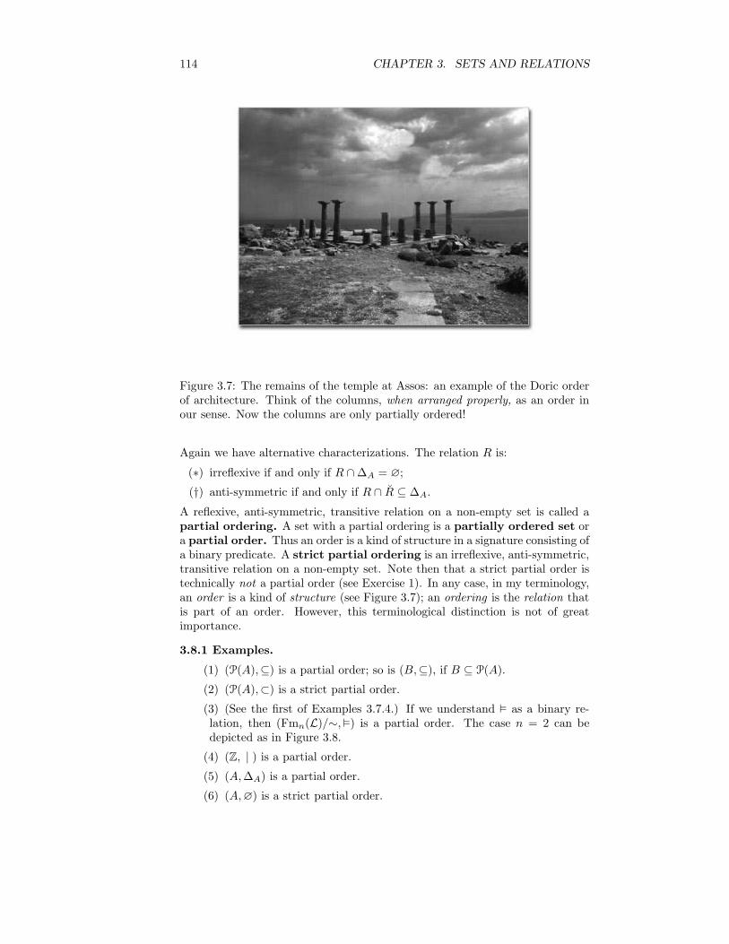
114 CHAPTER 3. SETS AND RELATIONS
Figure 3.7: The remains of the temple at Assos: an example of the Doric orderof architecture. Think of the columns, when arranged properly, as an order inour sense. Now the columns are only partially ordered!
Again we have alternative characterizations. The relation R is:
(∗) irreflexive if and only if R ∩∆A = ∅;
(†) anti-symmetric if and only if R ∩ R ⊆ ∆A.
A reflexive, anti-symmetric, transitive relation on a non-empty set is called apartial ordering. A set with a partial ordering is a partially ordered set ora partial order. Thus an order is a kind of structure in a signature consisting ofa binary predicate. A strict partial ordering is an irreflexive, anti-symmetric,transitive relation on a non-empty set. Note then that a strict partial order istechnically not a partial order (see Exercise 1). In any case, in my terminology,an order is a kind of structure (see Figure 3.7); an ordering is the relation thatis part of an order. However, this terminological distinction is not of greatimportance.
3.8.1 Examples.
(1) (P(A),⊆) is a partial order; so is (B,⊆), if B ⊆ P(A).
(2) (P(A),⊂) is a strict partial order.
(3) (See the first of Examples 3.7.4.) If we understand ² as a binary re-lation, then (Fmn(L)/∼,²) is a partial order. The case n = 2 can bedepicted as in Figure 3.8.
(4) (Z, | ) is a partial order.
(5) (A,∆A) is a partial order.
(6) (A,∅) is a strict partial order.

3.8. ORDERINGS 115
1
P ∨Q
oooooooooooooooooP → Q
²²²²²²²²Q→ P
////////
P | Q
JJJJJJJJJJJJJJ
Q
²²²²²²²²
oooooooooooooooooP
////////
oooooooooooooooooP = Q
JJJJJJJJJJJJ
oooooooooooooooP ↔ Q
////////
²²²²²²²²¬P
JJJJJJJJJJJJJ
²²²²²²²²¬Q
JJJJJJJJJJJJJ
////////
P ∧ Q
////////
²²²²²²²²
oooooooooooooooQ 9 P
JJJJJJJJJJJJJ
²²²²²²²²
ooooooooooooooooP 9 Q
JJJJJJJJJJJJJ
////////
ooooooooooooooooP fQ
JJJJJJJJJJJJ
////////
²²²²²²²²
0
JJJJJJJJJJJJJJ
////////
²²²²²²²²
ooooooooooooooooo
Figure 3.8: In this depiction of the set of (truth-equivalence-classes of) propo-sitional formulas in two variables, F ² G if an only if G can be reached from Fby travelling upwards along the drawn lines. The new connective 9 here hasthe obvious meaning.
(7) The relation 4 on sets is not a partial ordering; but we shall see in§ 4.8 that it ‘induces’ a partial ordering of cardinalities. •
3.8.2 Lemma.
(∗) If (A,R) is a partial ordering, then (A,R r ∆A) is a strict partialordering.
(†) If (A,S) is a strict partial ordering, then (A,S ∪ ∆A) is a partial or-dering.
Proof. Exercise.
In the lemma, one might say that R r ∆A is associated with R, and S ∪∆A
with S.
A partial order (A,R) is a total order (or a linear order) if
(A,R) ² ∀x ∀y (x R y ∨ y R x),
that is,
R ∪ R = A2.
If 6 is a total ordering, then the associated strict total ordering can be denotedby <, and vice versa.
3.8.3 Example. (Z,6) is a total order; (Z, <) is a strict total order. •

116 CHAPTER 3. SETS AND RELATIONS
Suppose (A,R) and (B,S) are partial orders, and f : A → B. Then f isorder-preserving if
x R y =⇒ f(x) S f(y)
for all x and y in A. An order-preserving function is an example of a moregeneral notion:
Suppose A and B are two structures in a signature L. A function f from A toB is called a homomorphism from A to B if
A ² φ(a0, . . . , an−1) =⇒ B ² φ(f(a0), . . . , f(an−1))
for all atomic formulas φ(x0, . . . , xn−1) of L and all ai in A, for all n in N.Moreover, f is an isomorphism if f is invertible and f−1 is a homomorphismfrom B to A.
A homomorphism is thus a function that preserves structure; it preserves thesymbols in a signature (hence it preserves the atomic formulas that use them).The existence of an isomorphism shows that two structures are the same asstructures. If an isomorphism exists between A and B, then A and B are calledisomorphic, and we write
A ∼= B.
Isomorphism is an equivalence-relation. Isomorphic structures have the sametheories.
3.8.4 Examples. Here are some kinds of homomorphisms and isomorphisms:
(1) An order-preserving function is a homomorphism of partial orders. Anisomorphism of partial orders is an invertible order-preserving functionwhose inverse is also order-preserving.
(2) Any function from a non-empty set to another is a homomorphism ofsets. Equipollence is isomorphism of sets.
(3) By Theorem 3.4.7, if f : A→ B, then X 7→ f−1[X] is a homomorphismfrom (P(B),∩,∪, c) to (P(A),∩,∪, c).
(4) More examples of homomorphisms and isomorphisms are in §§ 4.1, 4.3and 4.6. •
The following is a representation theorem: it shows that every partial ordercan be represented by (is isomorphic to) a structure of the form given in the firstof the Examples 3.8.1. Note how the proof of the theorem uses every propertyin the definition of partial orders.
3.8.5 Theorem. For every partial order (A,R), there is a set Ω and a subsetB of P(Ω) such that (A,R) ∼= (B,⊆). In fact, Ω can be A.
Proof. Let f be the function x 7→ y ∈ A : y R x from A to P(A). Then f isinjective: Indeed, suppose c and d are elements of A. If c R d and d R c, thenc = d since R is anti-symmetric. Suppose c 6= d. Then we may assume ¬(c R d).Then c /∈ f(d). But c ∈ f(c) since R is reflexive. Therefore f(c) 6= f(d). LetB = f [A]; then f gives a bijection between A and B.
Also, f is order-preserving: Suppose c R d. If e ∈ f(c), then e R c, so e R dsince R is transitive; hence e ∈ f(d). Thus f(c) ⊆ f(d). This shows that f isorder-preserving.

3.8. ORDERINGS 117
4 6
2
¡¡¡¡¡¡¡3 5
1
>>>>>>>
¡¡¡¡¡¡¡
1, 4 1, 2, 3, 6
1, 2
ssssssssss1, 3 1, 5
1
KKKKKKKKKK
ssssssssss
Figure 3.9: Two isomorphic partial orders:
But X 7→ f−1[X] is also order-preserving (as a function on B, this set beingequipped with the relation ⊆): If f(c) ⊆ f(d), then c ∈ f(d) since c ∈ f(c); soc R d.
Therefore f is an isomorphism from (A,R) to (B,⊆).
3.8.6 Examples.
(1) The partial ordering (1, 2, 3, 4, 5, 6, |) is isomorphic to (B,⊆), whereB is the set
1, 1, 2, 1, 3, 1, 2, 4, 5, 1, 2, 3, 6.
See Figure 3.9.
(2) A set of propositional formulas in n variables, partially ordered bylogical consequence (that is, by ²), is isomorphic to a set of Booleancombinations of n suitable sets, partially ordered by inclusion. CompareFigure 3.8 to Figure 3.10.
•
Exercises
(1) Show that no partial ordering is a strict partial ordering.
(2) Are there partial orders that are also equivalence-relations?
(3) Are there relations that are both symmetric and anti-symmetric?
(4) Write down the ordered pairs that belong to |, considered as a relation on1, 2, 3, 4, 5, 6. Can you add pairs to this relation so that it becomes atotal ordering?
(5) More generally, if R is a partial order on a finite set A, is there a totalordering S on A such that R ⊆ S?
(6) Find sets A and B such that all of the Boolean combinations depicted inFigure 3.10 are distinct.
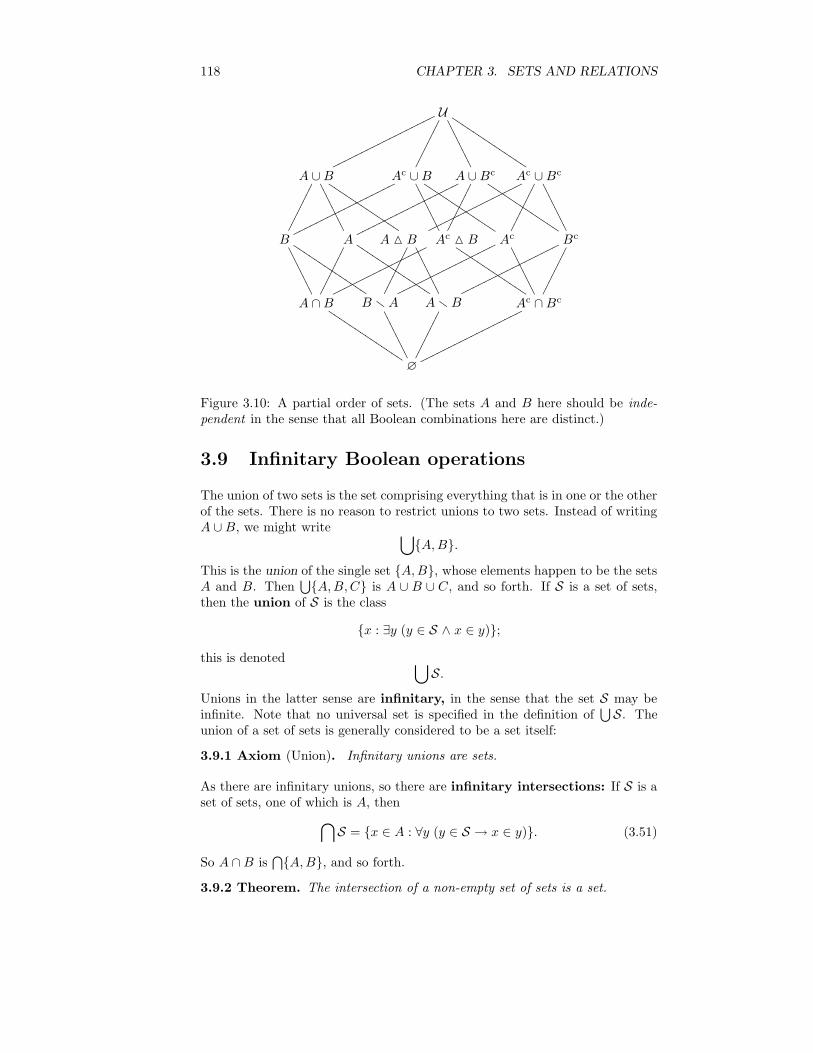
118 CHAPTER 3. SETS AND RELATIONS
U
A ∪B
ooooooooooooooooooAc ∪B
²²²²²²²²A ∪Bc
////////
Ac ∪Bc
JJJJJJJJJJJJJJ
B
²²²²²²²²
ooooooooooooooooooA
////////
ooooooooooooooooooA M B
JJJJJJJJJJJJJ
ooooooooooooooooAc M B
////////
²²²²²²²²Ac
JJJJJJJJJJJJJ
²²²²²²²²Bc
JJJJJJJJJJJJJ
////////
A ∩B
////////
²²²²²²²²
ooooooooooooooooB rA
JJJJJJJJJJJJJJ
²²²²²²²²
oooooooooooooooooArB
JJJJJJJJJJJJJJ
////////
oooooooooooooooooAc ∩Bc
JJJJJJJJJJJJJ
////////
²²²²²²²²
∅
JJJJJJJJJJJJJJ
////////
²²²²²²²²
oooooooooooooooooo
Figure 3.10: A partial order of sets. (The sets A and B here should be inde-pendent in the sense that all Boolean combinations here are distinct.)
3.9 Infinitary Boolean operations
The union of two sets is the set comprising everything that is in one or the otherof the sets. There is no reason to restrict unions to two sets. Instead of writingA ∪B, we might write ⋃
A,B.This is the union of the single set A,B, whose elements happen to be the setsA and B. Then
⋃A,B,C is A ∪ B ∪ C, and so forth. If S is a set of sets,then the union of S is the class
x : ∃y (y ∈ S ∧ x ∈ y);
this is denoted ⋃S.
Unions in the latter sense are infinitary, in the sense that the set S may beinfinite. Note that no universal set is specified in the definition of
⋃S. Theunion of a set of sets is generally considered to be a set itself:
3.9.1 Axiom (Union). Infinitary unions are sets.
As there are infinitary unions, so there are infinitary intersections: If S is aset of sets, one of which is A, then
⋂S = x ∈ A : ∀y (y ∈ S → x ∈ y). (3.51)
So A ∩B is⋂A,B, and so forth.
3.9.2 Theorem. The intersection of a non-empty set of sets is a set.

3.9. INFINITARY BOOLEAN OPERATIONS 119
Proof. By the Axiom of Separation, 1.2.3, the right member of Equation (3.51)is a set.
The following will be useful in the next chapter, starting in § 4.1.
3.9.3 Theorem. Let S be a set of sets, one of which is A. Then
⋂S ⊆ A ⊆
⋃S.
Proof. Exercise.
Sometimes, in an infinitary union⋃S (or an intersection
⋂S), the set S isgiven as the range of a function. Say f : A→ P(B). Then we can write
⋂f [A] =
⋂
x∈A
f(x)
and⋃f [A] =
⋃x∈A f(x).
3.9.4 Examples.
(∗) R =⋃n∈N
(−1− n, n+ 1);
(†) ⋂n∈N[n,∞) = ∅;
(‡) ⋂n∈N[−1/(n+ 1), 1/(n+ 1)] = 0.
Exercises
(1) Find⋃
∅ and⋃∅.
(2) Can you define⋂
∅?
(3) Find a set S of sets such that⋃S =
⋂S.
(4) Prove Theorem 3.9.3.
(5) Prove the infinitary analogues of some propositions in § 3.4: Supposef : A→ B, and S ⊆ P(A), and T ⊆ P(B). Then:
(a) f [⋃S] = ⋃f [X] : X ∈ S;
(b) f [⋂S] ⊆ ⋂f(X) : X ∈ S;
(c) the last inclusion is an equality if f is injective;
(d) f−1[⋃ T ] = ⋃f−1[X] : X ∈ T ;
(e) f−1[⋂ T ] = ⋂f−1[X] : X ∈ T .
Chapter 4
Numbers
4.0 The Peano axioms
In a book called The Principles of Arithmetic, Presented by a New Method [47],originally written in Latin and published in 1889, Giuseppe Peano describesthe positive integers by means of nine strings of symbols—strings that he callsaxioms. In our terminology, three of Peano’s axioms say that equality of pos-itive integers is an equivalence-relation; another says that everything equal toa positive integer is a positive integer. The remaining five axioms have moremathematical content, and versions of them are sometimes listed by themselves1
as the axioms for the positive integers; these axioms may or may not be calledthe Peano axioms. Two of these axioms say that 1 is a positive integer and thatevery positive integer has a successor that is a positive integer.
The remaining three of Peano’s axioms correspond to the three statements atthe end of § 1.2, except that the latter statements concern the natural numbers,rather than just the positive integers. In model-theoretic terms, Peano’s axiomsamount to the assertion that a certain structure is a model of the theory axiom-atized by certain sentences. (However, one of these sentences is second order.)I propose to make this an assertion about the natural numbers as follows:
4.0.1 Axiom (Existence of N). In the signature 0, +, there is a structure Nsuch that:
(∗) N ² ∀x x+ 6= 0;
(†) N ² ∀x ∀y (x+ = y+ → x = y);
(‡) (N, A) ² P0 ∧ ∀x (Px→ P (x+))→ ∀x Px, whenever A ⊆ N, and P isa singulary predicate.
(In the last line, it should be understood that A is to be considered as theinterpretation of P in N.) Henceforth, N is simply such a structure as namedin this Axiom.
I shall refer to the sentence ∀x x+ 6= 0 as Axiom Z, since it says that Z ero isnot a successor. Then ∀x ∀y (x+ = y+ → x = y) is Axiom U, since it says
1For example, in [23, pp. 988 f.] or [25, § 1].
120

4.0. THE PEANO AXIOMS 121
that successors are Unique when they exist. Finally, there is Axiom I, or theAxiom of Induction, a second-order sentence that can be written formally as
∀P (P0 ∧ ∀x (Px→ P (x+))→ ∀x Px),
where P is a singulary predicate-variable. Collectively, Axiom Z, Axiom U,and Axiom I can be called the Peano Axioms.
Axiom Z is that the immediate predecessor of 0 does not exist as an element ofN. The Axiom of Induction is that a set contains all natural numbers, providedthat it contains 0 and contains the successor of each natural number that itcontains. Later we shall define the binary operation (x, y) 7→ x+ y on N so thatx+ = x+ 1.
In § 1.2, I gave an informal definition of the set ω of von-Neumann naturalnumbers. The definition is such that the structure (ω, ′,∅) satisfies the Axiomof Induction automatically. In Theorems 1.2.4 and 1.2.6, we proved that thisstructure satisfies Axiom Z and Axiom U. Thus we proved the Axiom of Exis-tence of N, 4.0.1—on the assumption that ω exists. Now I want to justify thisassumption by means of another set-theoretic axiom:
4.0.2 Axiom (Infinity). There is a set Ω, consisting only of sets, such that∅ ∈ Ω, and for all sets A, if A ∈ Ω, then A′ ∈ Ω.
Let Ω be so. Then Ω contains all of what we have called the von-Neumannnatural numbers; but it may contain other things. We can throw out theseother things, obtaining ω itself, by taking an appropriate intersection. That is,we can make the definition
ω =⋂x ∈ P(Ω) : ∅ ∈ x ∧ ∀y (y ∈ x→ y ∪ y ∈ x). (4.1)
Now we can prove that ω has the properties claimed for it in § 1.2:4.0.3 Theorem. (ω, ′,∅) is a model of the Peano axioms.
Proof. Let S be the set whose intersection is defined to be ω in Equation 4.1.Then ω is a set by Theorem 3.9.2.
(∗) By definition, every element of S contains ∅; so ω contains ∅, the proofof Theorem 1.2.4 is valid, and ω satisfies Axiom Z.
(†) Every element of S also contains the set-theoretic successor of every setthat it contains; so ω satisfies Axiom U, by the proof of Theorem 1.2.6.
(‡) Finally, if A contains ∅, and contains the successor of its every element,then A ∈ S, and therefore ω ⊆ A by Theorem 3.9.3; so ω satisfies Axiom I.
Thus (ω, ′,∅) is a structure satisfying the Peano axioms.
We have now given a precise definition of the class ω defined informally in§ 1.2.2 We also observed in § 1.2 that, in ω, every non-zero von-Neumannnatural number is a successor; this is true generally in every model N of thePeano axioms, by the Axiom of Induction:
2More precisely, we have given two definitions—one less formal, one more—of structuressatisfying the Peano axioms. That only one structure can fit the definitions will be a conse-quence of Theorem 4.1.2.
122 CHAPTER 4. NUMBERS
4.0.4 Lemma. Every non-zero natural number is a successor. Symbolically,
N ² ∀x (x = 0 ∨ ∃y y+ = x).
Proof. Let A be the set of natural numbers comprising 0 and the successors.That is, A = 0 ∪ x ∈ N : ∃y y+ = x. Then 0 ∈ A by definition. Also, ifn ∈ A, then n+ is a successor, so n+ ∈ A. By induction, A = N.
In the last proof, the full inductive hypothesis n ∈ A was not needed; only n ∈ Nwas needed.
4.0.5 Theorem. The successor-operation is a bijection between N and Nr0;in particular,
N ≈ N r 0.
Proof. Exercise.
By the definition suggested by Richard Dedekind3 in 1882, a set is infinite if itis equipollent with a proper subset of itself. (See also § 4.8.) Then we have:
4.0.6 Corollary. N is infinite.
Proof. Immediate from the theorem.
4.0.7 Lemma. Every natural number is distinct from its successor:
N ² ∀x x+ 6= x.
Proof. Let A = x ∈ N : x+ 6= x. Now, 0+ is a successor and is thereforedistinct from 0 by Axiom Z. Hence 0 ∈ A. Suppose n ∈ A. Then n+ 6=n. Therefore n++ 6= n+ by the contrapositive of Axiom U; so n+ ∈ A. Byinduction, A = N.
4.1 Recursion
To able to say much more about the natural numbers, we should introduce theusual arithmetic operations. We need not do this by axioms; we can define theoperations. But how? There are several possible approaches. The approachthat I propose to take starts with the following theorem. Its proof is difficult,but once we have the theorem, then we can freely define many useful operationsand functions.
4.1.1 Theorem (Recursion). Suppose B is a set with an element c, and f :B → B. Then there is a unique function g from N to B such that g(0) = c and
g(n+) = f(g(n)) (4.2)
for all n in N.
3See Dedekind’s note on [9, p. 63].
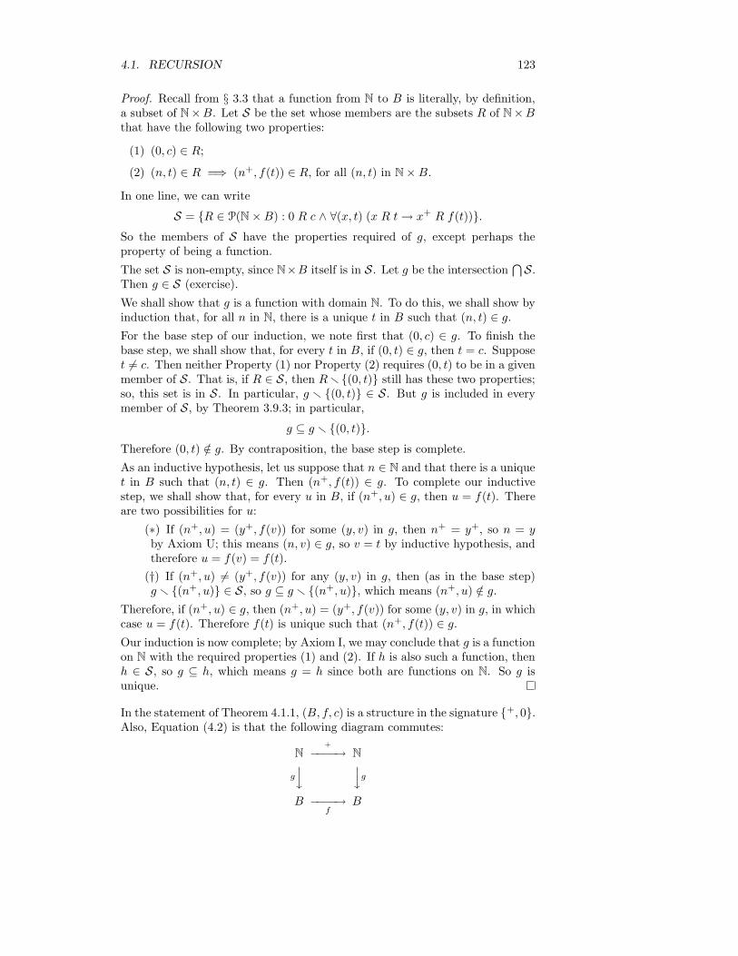
4.1. RECURSION 123
Proof. Recall from § 3.3 that a function from N to B is literally, by definition,a subset of N×B. Let S be the set whose members are the subsets R of N×Bthat have the following two properties:
(1) (0, c) ∈ R;(2) (n, t) ∈ R =⇒ (n+, f(t)) ∈ R, for all (n, t) in N×B.
In one line, we can write
S = R ∈ P(N×B) : 0 R c ∧ ∀(x, t) (x R t→ x+ R f(t)).So the members of S have the properties required of g, except perhaps theproperty of being a function.
The set S is non-empty, since N×B itself is in S. Let g be the intersection⋂S.
Then g ∈ S (exercise).
We shall show that g is a function with domain N. To do this, we shall show byinduction that, for all n in N, there is a unique t in B such that (n, t) ∈ g.For the base step of our induction, we note first that (0, c) ∈ g. To finish thebase step, we shall show that, for every t in B, if (0, t) ∈ g, then t = c. Supposet 6= c. Then neither Property (1) nor Property (2) requires (0, t) to be in a givenmember of S. That is, if R ∈ S, then Rr (0, t) still has these two properties;so, this set is in S. In particular, g r (0, t) ∈ S. But g is included in everymember of S, by Theorem 3.9.3; in particular,
g ⊆ g r (0, t).Therefore (0, t) /∈ g. By contraposition, the base step is complete.
As an inductive hypothesis, let us suppose that n ∈ N and that there is a uniquet in B such that (n, t) ∈ g. Then (n+, f(t)) ∈ g. To complete our inductivestep, we shall show that, for every u in B, if (n+, u) ∈ g, then u = f(t). Thereare two possibilities for u:
(∗) If (n+, u) = (y+, f(v)) for some (y, v) in g, then n+ = y+, so n = yby Axiom U; this means (n, v) ∈ g, so v = t by inductive hypothesis, andtherefore u = f(v) = f(t).
(†) If (n+, u) 6= (y+, f(v)) for any (y, v) in g, then (as in the base step)g r (n+, u) ∈ S, so g ⊆ g r (n+, u), which means (n+, u) /∈ g.
Therefore, if (n+, u) ∈ g, then (n+, u) = (y+, f(v)) for some (y, v) in g, in whichcase u = f(t). Therefore f(t) is unique such that (n+, f(t)) ∈ g.Our induction is now complete; by Axiom I, we may conclude that g is a functionon N with the required properties (1) and (2). If h is also such a function, thenh ∈ S, so g ⊆ h, which means g = h since both are functions on N. So g isunique.
In the statement of Theorem 4.1.1, (B, f, c) is a structure in the signature +, 0.Also, Equation (4.2) is that the following diagram commutes:
N+
−−−−→ N
g
yyg
B −−−−→f
B
124 CHAPTER 4. NUMBERS
That is, from the N on the left to the B on the right, there are two differentroutes, but each one yields the same result. In fact, the theorem is simply thatthere is a unique homomorphism from (N,+, 0) to (B, f, c).
A recursive definition, or a definition by recursion, is a definition of afunction on N that is justified by Theorem 4.1.1. Informally, we can define sucha function g by specifying g(0) and by specifying how g(n+) is obtained fromg(n).
Sections 4.2 and 4.4 will provide several important examples of recursive defini-tions. Such definitions are sometimes4 called inductive definitions, or definitionsby induction. However, this terminology is misleading when Axiom I is calledthe Axiom of Induction. Logically, the Recursion Theorem is equivalent to thethree Peano Axioms together; the Recursion Theorem is strictly stronger thanthe Induction Axiom, in the sense that there are models of Axiom I that do notsatisfy Theorem 4.1.1. The remainder of this section is devoted to proving this.
Let us say that a structure admits (definition by) recursion if it satisfiesthe Recursion Theorem. That is, a structure A in the signature +, 0 admitsrecursion if and only if, for any other structure B in this signature, there is aunique homomorphism from A to B.
Similarly, structures that satisfy the Induction Axiom can be said to admit(proof by) induction.
4.1.2 Theorem. All structures that admit recursion are isomorphic.
Proof. Suppose A and B admit recursion. Then there are unique homomor-phisms f from A to B and g from B to A. Hence the composition g f is ahomomorphism from A to itself; so it is the unique such homomorphism. ButidA is also such a homomorphism. Therefore g f = idA. Similarly, f g = idB .Therefore g = f−1, by Theorem 3.3.4.
4.1.3 Corollary. All structures that admit recursion satisfy the Peano axioms;in particular, they admit induction.
Proof. By the theorem, every structure that admits recursion is isomorphicto (N,+, 0). This satisfies the Peano axioms; hence so does every structureisomorphic to it.
However, there are structures that admit induction, but not recursion:5
4Dedekind calls them definitions by induction in [9, Theorem 126, p. 85], which correspondsto the Recursion Theorem above.
5Apparently Peano himself did not recognize the distinction between proof by inductionand definition by recursion; see the discussion on [25, p. x]. Burris does not acknowledgethe distinction; see [5, p. 391]. Stoll [40, p. 72] uses the term ‘definition by weak recursion’,although he observes that the validity of such a definition does not obviously follow from theInduction Axiom. However, Stoll does not prove (as we have done in Example 4.1.4) that theInduction Axiom is consistent with the negation of the Recursion Theorem.

4.2. THE ARITHMETIC OPERATIONS 125
4.1.4 Example. On B, define a singulary operation s by s(0) = 1 and s(1) = 0.Then (B, s, 0) admits induction,6 but there is no function g : B → N such thatg(0) = 0 and g(s(n)) = (g(n))+ for all n in B.
Exercises
(1) If g and S are as in the proof of the Recursion Theorem, prove that g ∈ S.(2) Prove directly (without Theorem 4.1.2) that Axiom Z is a consequence of
the Recursion Theorem. (For example, if in A the successor-operation issurjective, show that there is no homomorphism from A into N.)
4.2 The arithmetic operations
By recursion, we can define addition, multiplication and exponentiation.7 First,we define the binary operation + of addition on N by defining, for each n inN, the singulary operation y 7→ n+ y. This operation is given by the rules:
(∗) n+ 0 = n;
(†) n+m+ = (n+m)+.
4.2.1 Lemma. N satisfies
(∗) ∀x 0 + x = x,
(†) ∀x ∀y y+ + x = (y + x)+.
Proof. By definition of addition, 0 + 0 = 0. Suppose 0 + n = n. Then
0 + n+ = (0 + n)+ [by definition of addition]
= n+. [by inductive hypothesis]
This completes an induction showing ² ∀x 0 + x = x.
For the second claim, as the base step of an induction, we have
m+ + 0 = m+ [by the first claim]
= (m+ 0)+; [again by the first claim]
6The structure (B, s, 0) in Example 4.1.4 also satisfies Axiom U, but not Axiom Z. If wedefine t : B → B so that t(n) = 1 for each n in B, then (B, t, 0) satisfies the Induction Axiomand Axiom Z, but not Axiom U. Later we shall have natural examples of structures satisfyingAxiom Z and Axiom U, but not admitting induction.
7We can also define addition and multiplication using only the Induction Axiom, not theRecursion Theorem. The method is shown, for example, in [25]. As a result, the operationscan be defined on structures that do not satisfy all of the Peano Axioms. For example, let nbe a positive integer, and on Z let ≡ be congruence modulo n. if x ≡ y, then x + 1 ≡ y + 1(though by the standards of this chapter, we can’t quite prove this yet). Hence we can definea successor-operation s, namely
[x] 7−→ [x + 1] : Z/≡ −→ Z/≡.
The resulting structure (Z/≡, s, [0]) satisfies the Induction Axiom; therefore it can be equippedwith an addition and a multiplication that satisfy the theorems of this section. (The result isarithmetic modulo n.) We cannot in general define exponentiation on Z/≡. If we try to dothis in case n = 3, we get 20 = 1, 21 = 2, 22 = 2 · 2 = 1, so 2s(2) = 2—but also s(2) = 0, so2s(2) = 20 = 1.

126 CHAPTER 4. NUMBERS
so ∀y y+ + 0 = (y + 0)+.
Now, as an inductive hypothesis, suppose ∀y y+ + n = (y + n)+. Then, for allm in N, we have
m+ + n+ = (m+ + n)+ [by definition of addition]
= (m+ n)++ [by inductive hypothesis]
= (m+ n+)+ [again by definition of addition].
This completes an induction showing ∀x ∀y y+ + x = (y + x)+.
The second part of the proof showed N = x : ∀y y+ + x = (y + x)+: We haveproved the identity
y+ + x = (y + x)+ (4.3)
in N by induction on x. Induction on y here does not work directly. Indeed,suppose A = y ∈ N : ∀x y+ + x = (y + x)+. To prove that 0 ∈ A, we have toshow that 0+ +n = (0+n)+. From the first part of the theorem, we know that(0 + n)+ = n+; but we cannot yet say anything about 0+ + n. We could prove∀x 0+ + x = x+ by induction; but it would be more efficient just to start overand prove Identity (4.3) by induction on x.
To prove some identities below, one has to choose the right variable to workwith.
4.2.2 Theorem. N satisfies
(∗) ∀x x+ = x+ 1;
(†) ∀x ∀y x+ y = y + x [that is, + is commutative];
(‡) ∀x ∀y ∀z (x+ y) + z = x+ (y + z) [that is, + is associative];
(§) ∀x ∀y ∀z (x+ z = y + z → x = y) [that is, + admits cancellation].
Proof. Exercise.
The binomial coefficients(nm
)are given by a two-stage recursion:
(∗)(00
)= 1, and
(0m+
)= 0.
(†)(n+
0
)= 1, and
(n+
m+
)=(nm
)+(nm+
).
(See also Exercises 6 and 7 in § 4.5.)The binary operation · of multiplication on N is given by:
(∗) n · 0 = 0
(†) n ·m+ = n ·m+ n.
Multiplication is also indicated by juxtaposition, so that n ·m is nm.
4.2.3 Lemma. N satisfies
(∗) ∀x 0x = 0,
(†) ∀x ∀y y+x = yx+ x.
Proof. Exercise.

4.3. THE INTEGERS AND THE RATIONAL NUMBERS 127
4.2.4 Theorem. N satisfies
(∗) ∀x 1x = x,
(†) ∀x ∀y xy = yx [that is, · is commutative],
(‡) ∀x ∀y ∀z (x+ y)z = xz + yz [that is, · distributes over +],
(§) ∀x ∀y ∀z (xy)z = x(yz) [that is, · is associative].
Proof. Exercise.
Finally, exponentiation: the binary operation (x, y) 7→ xy on N is given by:
(∗) n0 = 1;
(†) nm+
= nm · n.
4.2.5 Theorem. The following are identities in N:
(∗) xy+z = xyxz;
(†) (xy)z = xyz;
(‡) (xy)z = xzyz.
Proof. Exercise.
Exercises
(1) Prove Lemma 4.2.2. In the latter two parts, does induction work on everyvariable?
(2) Prove that(x1
)= x for all x in N.
(3) Prove Lemma 4.2.3. In the second part, does induction work on eithervariable?
(4) Prove Theorem 4.2.4.
(5) Prove Theorem 4.2.5.
4.3 The integers and the rational numbers
In Examples 3.7.1 and 3.7.4, I mentioned equivalence-relations ∼ on N×N and≈ on Z× (Z r 0) and corresponding bijections:
(∗) [a, b] 7−→ a− b from N2/∼ to Z;
(†) [a, b] 7−→ a/b from Z× (Z r 0)/≈ to Q.
We couldn’t properly prove these claims then, since we didn’t have precise def-initions of the structures involved. Now that we have defined N axiomatically,we can use the observations in § 3.7 to justify a definition of Z and Q in termsof N.
128 CHAPTER 4. NUMBERS
4.3.1 Lemma. On N× N, let ∼ be the relation given by
(a, b) ∼ (c, d) ⇐⇒ a+ d = b+ c.
Then ∼ is an equivalence-relation. If (a0, b0) ∼ (a1, b1) and (c0, d0) ∼ (c1, d1),then
(∗) (a0 + c0, b0 + d0) ∼ (a1 + c1, b1 + d1);
(†) (b0, a0) ∼ (b1, a1);
(‡) (a0c0 + b0d0, b0c0 + a0d0) ∼ (a1c1 + b1d1, b1c1 + a1d1).
Proof. Exercise. For the last part, show that each member is equivalent to(a1c0 + b1d0, b1c0 + a1d0).
Letting ∼ be as in Lemma 4.3.1, we now define Z to be N × N/∼. Let the∼-class of (a, b) be denoted
a− b.By Theorem 3.7.3 and Lemma 4.3.1, we can define the operations +, −, and · onZ by the following rules, where a, b, c, d ∈ N. I use superscripts on the symbols(as described in § 3.5) as a reminder of which structure is being considered:
(∗) (a− b) +Z (c− d) = (a+N c)− (b+N d);
(†) −Z(a− b) = b− a;(‡) (a− b) ·Z (c− d) = (a ·N c+N b ·N d)− (b ·N c+N a ·N d).
Alternatively,
(∗) Addition on Z is (x− y, z − w) 7→ (x+ z)− (y + w);
(†) additive inversion on Z is x− y 7→ y − x;(‡) multiplication on Z is (x− y, z − w) 7→ (xz + yw)− (yz + xw).
Note that, by the current precise definition, an integer like 5 − 3 is not thenatural number 2; it is not a natural number at all; it is the equivalence-class
(2, 0), (3, 1), (4, 2), (5, 3), . . . ,
which is (x, y) ∈ N2 : x = y + 2. The distinction is just a technical detail,because of the following:
4.3.2 Theorem. Let i be the function x 7→ x − 0 from N to Z. Then i isinjective. Also, i is a homomorphism from (N,+, · ) to (Z,+, · ), that is,
(∗) i(a+N b) = i(a) +Z i(b);
(†) i(a ·N b) = i(a) ·Z i(b)for all a and b in N. On Z, addition and multiplication are commutative andassociative, and multiplication distributes over addition. Finally,
a+Z (−Za) = 0− 0 = i(0)
for all a in Z.
Proof. Exercise.

4.3. THE INTEGERS AND THE RATIONAL NUMBERS 129
On Z, define the binary operation − by the identity
x− y = x+ (−y).
4.3.3 Lemma. If a, b ∈ N, then the integer a− b is (a− 0)−Z (b− 0).
Proof. Exercise.
Now we can identify the natural numbers with their images in Z, consideringthe natural number n to be equal to the integer n− 0.
We can define the rational numbers similarly:
4.3.4 Lemma. On Z× (Z r 0), let ≈ be the relation given by
(a, b) ≈ (c, d) ⇐⇒ ad = bc.
Then ≈ is an equivalence-relation. If (a0, b0) ≈ (a1, b1) and (c0, d0) ≈ (c1, d1),then
(∗) (a0d0 ± b0c0, b0d0) ≈ (a1d1 ± b1c1, b1d1);
(†) (a0c0, b0d0) ≈ (a1c1, b1d1);
(‡) (b0, a0) ≈ (b1, a1) and (0, a0) ≈ (0, 1) if a0 6= 0.
Proof. Exercise.
Letting ≈ be as in Lemma 4.3.4, we define Q to be Z × (Z r 0)/≈. Let the≈-class of (a, b) be denoted
a
b
or a/b. By Theorem 3.7.3 and Lemma 4.3.4, we can define the operations +,−, and · on Q, and x 7→ x−1 on Q r 0/1, by the following rules, wherea, b, c, d ∈ Z:
(∗) a/b± c/d = (ad± bc)/bd;(†) (a/b)(c/d) = ac/bd;
(‡) (a/b)−1 = b/a if a 6= 0.
4.3.5 Theorem. The function x 7→ x/1 is an injective homomorphism from(Z,+,−, · ) to (Q,+,−, · ). On Q, addition and multiplication are commutativeand associative, and multiplication distributes over addition. Finally,
a · a−1 =1
1
for all a in Q r 0/1.
Proof. Exercise.
Now we can identify the integers with their images in Q, considering the integerx to be equal to the rational number x/1.

130 CHAPTER 4. NUMBERS
Exercises
(1) Prove Lemma 4.3.1.
(2) Prove Theorem 4.3.2.
(3) Prove Lemma 4.3.3.
(4) Prove Lemma 4.3.4.
(5) Prove Theorem 4.3.5.
4.4 Recursion generalized
How can we define n!, called n-factorial? Informally, we write
n! = 1 · 2 · 3 · · · (n− 1) · n.
A formal recursive definition should be able to take care of the dots. We say0! = 1, and (n+)! = n+ ·n!. But for this to be a valid definition by the RecursionTheorem, we would have to express n+ · n! as a function of n!.
In fact our definition of n! is valid by the following.
4.4.1 Theorem (Recursion with Parameter). Suppose B is a set with an ele-ment c, and F : N × B → B. Then there is a unique function G from N to Bsuch that G(0) = c and
G(n+) = F (n,G(n)) (4.4)
for all n in N.
Proof. Let f be the function
(x, b) 7−→ (x+, F (x, b))
from N × B to N × B. By recursion, there is a unique function g from N toN×B such that g(0) = (0, c) and
g(n+) = f(g(n))
for all n in N. Now let G be π g, where π is the function
(x, b) 7−→ b
from N× B to B. Then for each n in N we have g(n) = (m,G(n)) for some min N. We can prove by induction that m = n. Indeed, this is the case whenn = 0, since g(0) = (0, c). Suppose g(n) = (n,G(n)) for some n in N. Then
g(n+) = f(n,G(n)) = (n+, F (n,G(n))). (4.5)
In particular, the first entry in the value of g(n+) is n+. This completes ourinduction.
We now know that g(n) = (n,G(n)) for all n in N. Hence in particular g(n+) =(n+, G(n+)). But we also have (4.5). Therefore we have (4.4), as desired.Finally, each of g and G determines the other. Since g is unique, so is G.
4.5. THE ORDERING OF THE NATURAL NUMBERS 131
4.4.2 Example. We can define a function f on N by requiring f(0) = 0 andf(x+) = x. This is a valid recursive definition, by Theorem 4.4.1. Note that fpicks out the immediate predecessor of a natural number, when this exists.8
For any function f from N to M , where M is a set equipped with additionand multiplication, we can now define the sum
∑n
k=0 f(k) and the product∏nk=0 f(k) recursively as follows:
(∗)0∑
k=0
f(k) = f(0) and
n+∑
k=0
f(k) =
n∑
k=0
f(k) + f(n+);
(†)0∏
k=0
f(k) = f(0) andn+∏
k=0
f(k) =
(n∏
k=0
f(k)
)f(n+).
See Exercise 1 below.
Exercises
(1) Show clearly that the definitions of∑n
k=0 f(k) and∏n
k=0 f(k) are justifiedby Theorem 4.4.1.
(2) Prove the following for all n in N:
(a)∑n
k=0(k + 1) = (n2 + 3n+ 2)/2;
(b)∑n
k=0(k + 1)2 = (2n3 + 9n2 + 13n+ 6)/6;
(c)∑n
k=0 bk = (bn+1 − 1)/(b− 1);
(d)∑n
k=0(2k + 1) = (n+ 1)2;
(e)∏n
k=0((k + 1)/(k + 2)) = 1/(n+ 2).
4.5 The ordering of the natural numbers
We can define the binary relation 6 on N as the set
(x, y) ∈ N× N : ∃z x+ z = y.
The associated strict relation < is then (x, y) ∈ N× N : x 6 y ∧ x 6= y. Nowwe have to show that 6 is the total ordering that we expect:
4.5.1 Lemma. N ² ∀x ∀y (x+ 6 y+ → x 6 y).
Proof. Suppose a+ 6 b+. Then a+ + c = b+ for some c in N, by definition of6. This means (a+ c)+ = b+, by Lemma 4.2.1, so a+ c = b, by Axiom U, andtherefore a 6 b, again by the definition of 6.
4.5.2 Lemma. N satisfies:
(∗) ∀x (x 6 0→ x = 0);
(†) ∀x ∀y (x+ y 6 x→ y = 0).
8Since f is unique, we now have a proof that Axiom U follows from the Recursion Theorem.
132 CHAPTER 4. NUMBERS
Proof. Suppose a 6 0. Then a+ b = 0 for some b in N. Either a = 0, or a = c+
for some c in N, by Lemma 4.0.4. In the latter case, (c + b)+ = 0, which isabsurd by Axiom Z. Hence a = 0, and the first claim is proved.
Now suppose a + b 6 a. Then a + b + c = a = a + 0 for some c, so b + c = 0by cancellation (Theorem 4.2.2), which means b 6 0. Hence b = 0 by the firstclaim. The second claim is now proved.
4.5.3 Lemma. N satisfies:
(∗) ∀x ∀y (x < y → x+ 6 y);
(†) ∀x ∀y (x < y+ → x 6 y).
Proof. To prove the first claim, by Lemma 4.0.4, it is enough to show
∀x (x < 0→ x+ 6 0),
∀x ∀y (x < y+ → x+ 6 y+).
The first sentence is trivially true in N by Lemma 4.5.2, since the hypothesisx < 0 always fails: If n < 0, then n 6 0, so n = 0, which means ¬(n < 0).
For the second sentence, suppose n < m+. Then n + ` = m+ for some `; but` 6= 0, so ` = k+ for some k. Hence n + k+ = m+, that is, n+ + k = m+, son+ 6 m+.
The proof of the second claim is an exercise.
4.5.4 Theorem. On N, the relation 6 is a total ordering.
Proof. There are four properties to check:
Reflexivity: Since n+ 0 = n, we have n 6 n by definition.
Anti-symmetry: We can use Lemma 4.0.4. If n 6 0 and 0 6 n, then n 6 0,so n = 0 by Lemma 4.5.2. Suppose n 6 m+ and m+ 6 n. From the latterinequality, n = m+ + ` = (m + `)+ for some `. Hence (m + `)+ 6 m+
by the former inequality, so m+ ` 6 m by Lemma 4.5.1. Hence ` = 0 byLemma 4.5.2, so n = m+ + 0 = m+.
Transitivity: If n 6 m and m 6 0, then m = 0 by Lemma 4.5.2, so n 6 0,so n = 0. As an inductive hypothesis, suppose
∀x ∀y (x 6 y ∧ y 6 `→ x 6 `).
Suppose also n 6 m and m 6 `+. There are two possibilities. If m = `+,then n 6 `+. Suppose m < `+. Then m 6 ` by Lemma 4.5.3, so n 6 `by inductive hypothesis. By definition then, n + k = ` for some k, son+ k+ = `+, and therefore n 6 `+. This completes the induction.
Totality: We shall prove x 6 y∨y 6 x by induction on x. Since 0+m = mfor all m, we have ∀y 0 6 y. As an inductive hypothesis, suppose
∀y (n 6 y ∨ y 6 n).
To complete the induction, suppose ¬(n+ 6 m) for some m. Then ¬(n <m) by Lemma 4.5.3. By inductive hypothesis, m 6 n. Also n 6 n + 1 =n+. By transitivity, m 6 n+.
4.5. THE ORDERING OF THE NATURAL NUMBERS 133
The proof is complete.
Various standard properties can now be proved:
4.5.5 Theorem. N satisfies:
(∗) ∀x 0 6 x;
(†) ∀x ∀y ∀z (x < y ↔ x+ z < y + z);
(‡) ∀x ∀y ∀z (x < y → x · z+ < y · z+);
(§) ∀x ∀y ∃z (x 6 y ↔ x+ z = y).
Proof. Exercise.
Exercises
(1) Complete the proof of Lemma 4.5.3.
(2) Prove Theorem 4.5.5.
(3) Prove N ² ∀x x < 2x. (See § 3.6 (3.50).)
(4) Prove the following in N.
(∗) ∀x ∀y 1 + xy 6 (1 + x)y
(†) ∀x (3 < x→ x2 < 2x)
(5) Find the flaw in the following argument, where max is the function fromN×N to N such that max(x, y) = y if x 6 y, and otherwise max(x, y) = x.
If max(x, y) = 0, then x = y. Suppose that x = y whenevermax(x, y) = n. Suppose max(z, w) = n + 1. Then max(z −1, w−1) = n, so z−1 = w−1 by inductive hypothesis; thereforez = w. Therefore all natural numbers are equal.
(6) Prove that, if y 6 x, then
(x
y
)=
x!
y! (x− y)! .
(7) Prove the Binomial Theorem:
(x+ y)n =
n∑
i=0
(n
i
)xn−iyi.
(8) Prove that every proper divisor of a positive integer is less than thatinteger. (By proper divisor, I mean a divisor other than the numberitself.)

134 CHAPTER 4. NUMBERS
4.6 The real numbers
Recall from § 4.3 that every integer is a difference x−y of two natural numbers,and every rational number is a quotient u/v of two integers.
4.6.1 Lemma. There is a well-defined subset P of Z consisting of those differ-ences a− b of natural numbers a and b such that b < a. There is a unique stricttotal ordering < of Z such that
x < y ⇐⇒ y − x ∈ P
for all x and y in Z. The injection x 7→ x− 0 : N → Z is order-preserving.
4.6.2 Lemma. There is a well-defined subset P of Q consisting of those quo-tients a/b of integers a and b such that 0 < ab. There is a unique strict totalordering < of Q such that
x < y ⇐⇒ y − x ∈ P
for all x and y in Q. The injection x 7→ x/1 : Z → Q is order-preserving.
A cut of a total order (X,6) is a subset a such that:
(∗) ∅ ⊂ a ⊂ X;
(†) x < y ∧ y ∈ a =⇒ x ∈ a;
(‡) ∀y (y ∈ a → y 6 x) =⇒ x /∈ a.
The set R of real numbers is the set of cuts of Q. On R, the operations +and · and the relation < can be defined so that the expected algebraic propertiesare true. Details are an exercise.
4.6.3 Theorem. The function x 7→ y ∈ Q : y < x : Q → R is an injectivehomomorphism from (Q,+, · , <) to (R,+, · , <).
Proof. Exercise.
If a, b ∈ R, then [a, b) is the set x ∈ R : a 6 x < b.4.6.4 Theorem. Suppose the real number a is in [0, 1). Then there is a uniquefunction k 7→ ak : N → B such that
n∑
k=0
ak2k+1
6 a <
n∑
k=0
ak2k+1
+1
2n+1
for all n in N.
Proof. Exercise.
With notation as in the theorem, we can write
a =∑
k∈N
ak2k+1
;
this is a binary expansion of a.

4.7. WELL-ORDERED SETS 135
4.7 Well-ordered sets
Suppose (Ω,6) is a total order. Then we can define a function x 7→ predx fromΩ to P(Ω) by the rule
predx = y ∈ Ω : y < x.Then pred a is the set of predecessors of a. Suppose A ⊆ Ω. An element b ofΩ is a least or minimal element of A if b ∈ A, but b 6 c if c ∈ A. That is, anelement b of Ω is a least element of A if and only if
b ∈ A & A ∩ pred a = ∅.
4.7.1 Lemma. Least elements are unique when they exist.
Proof. Exercise.
The least element—if it exists—of a subset A can be denoted
minA.
The total order (Ω,6):
(∗) is well-ordered if every non-empty subset of Ω has a least element;
(†) admits (proof by) strong induction if A = Ω whenever A is a subsetof Ω such that
pred b ⊆ A =⇒ b ∈ Afor all b in Ω;
(‡) admits (definition by) strong recursion if, for every set B and func-tion h from P(B) to B, there is a unique function G from Ω to B suchthat
G(c) = h(G[pred c])
for all c in Ω.
We shall see presently that these three conditions are equivalent. Meanwhile,we can observe that (N,6) satisfies one of the conditions.
4.7.2 Lemma. pred (n+) = predn ∪ n for all n in N.
Proof. Since n < n+, we have predn ∪ n ⊆ pred (n+). For the reverse in-clusion, suppose a ∈ pred (n+), so that a < n+. Then a 6 n by Lemma 4.5.3,so a = n or a < n; in either case, a ∈ predn ∪ n. Thus, pred (n+) ⊆predn ∪ n.
4.7.3 Theorem. (N,6) admits strong induction.
Proof. Suppose A is a subset of N that contains n whenever it includes predn.By induction, we shall show that predn ⊆ A for all n in N, and then A = N.
Since pred 0 = ∅, and ∅ ⊆ A, this means 0 ∈ A by assumption. As aninductive hypothesis, suppose predn ⊆ A. Then n ∈ A by assumption, sopred (n+) = predn ∪ n ⊆ A by Lemma 4.7.2. This completes the induction.Hence, for all n, we have n ∈ pred (n+) ⊆ A, so n ∈ A. Thus A = N.
136 CHAPTER 4. NUMBERS
Example 4.7.7 will show one use of strong induction.
The totally ordered set (Ω,6) is well-ordered if and only if every subset with noleast element is empty. This formulation will be used in proving the followingtheorem. Also, a subset A of Ω has no least element if and only if
∀x (predx ∩A = ∅ → x /∈ A),
that is, ∀x (predx ⊆ Ω rA→ x ∈ Ω rA).
4.7.4 Theorem. The following are equivalent conditions on a total order:
(∗) It is well-ordered.
(†) It admits strong induction.
(‡) It admits strong recursion.
Proof. Let (Ω,6) be a total order. We shall show that, if it admits stronginduction or strong recursion, then it is well-ordered, and if it is well-ordered,then it admits strong induction and strong recursion.
Suppose (Ω,6) admits strong induction, but A is a subset of Ω with no leastelement. We shall show that A is empty. If a ∈ Ω, and pred a ⊆ Ω r A, thena ∈ ΩrA, since a is not a least element of A. By strong induction, Ω = ΩrA,so A = ∅. Thus (Ω,6) is well-ordered.
Suppose (Ω,6) admits strong recursion, but A is a subset of Ω with no leastelement. Let
C = x ∈ Ω : ∃y (y ∈ A ∧ y 6 x).Then C has no least element (exercise). For each e in B, let Ge be the functionfrom Ω to B given by
Ge(x) =
0, if x /∈ C;e, if x ∈ C.
(So G1 is the characteristic function of C on Ω in the sense of § 3.6, but G0 isthe constant function x 7→ 0 on Ω.) Let h be the function from P(B) to B givenby
h(X) = 1 ⇐⇒ 1 ∈ X,that is,
h(X) =
0, if X ∈ ∅, 0;1, if X ∈ 1, 0, 1.
Then G(a) = h(G[pred a]) for all a in Ω, whether G is G0 or G1 (exercise). Bystrong recursion, there is a unique such function G, so G0 = G1. ThereforeC = ∅. Thus (Ω,6) is well-ordered.
Now, conversely, suppose (Ω,6) is well-ordered. First, let A be a subset ofΩ such that, if pred a ⊆ A, then a ∈ A, for all a in A. Consequently, ifpred a ∩ (Ω r A) = ∅, then a /∈ Ω rA. Then Ω r A has no least element, so itis empty, and A = Ω. Thus (Ω,6) admits strong induction.
Finally, using that (Ω,6) admits strong induction, we shall follow the proofof the Recursion Theorem, 4.1.1, to prove that (Ω,6) admits strong recursion.

4.7. WELL-ORDERED SETS 137
Suppose B is a set, and h : P(B)→ B. Let S be the set of relations R from Ωto B such that
(a, h(f [pred a])) ∈ Rwhenever f : pred a → B and f ⊆ R. Then S is non-empty, since it containsΩ×B itself. Let G =
⋂S. Then G ∈ S (exercise). Let
A = x ∈ Ω : ∃! y (x, y) ∈ G.
Suppose pred a ⊆ A. Then G ∩ (pred a × B) is the unique function f frompred a to B such that f ⊆ G. Hence (exercise) h(f [pred a]) is the unique b inB such that (a, b) ∈ G. Therefore a ∈ A. By strong induction, A = Ω, so G isa function from Ω to B. Also,
G(a) = h(G[pred a])
for all a in Ω, since G ∈ S. Suppose G′ is another function on Ω in S. Let
D = x ∈ Ω : G(x) = G′(x).
If pred a ⊆ D, then G′(a) = h(G′[pred a]) = h(G[pred a]) = G(a), so a ∈ D. Bystrong induction, D = Ω, so G′ = G. Thus G is the only function on Ω in S,and (Ω,6) admits strong recursion.
4.7.5 Corollary. (N,6) is well-ordered and admits strong recursion.
Proof. Theorem 4.7.3.
Interrelations
What is the force of the word strong in strong induction and strong recursion?
Structures that admit induction or recursion have a signature that includes+, 0. Structures that admit strong induction or strong recursion have a sig-nature that includes 6. The next theorem establishes one connexion betweenthese two kinds of structures:
4.7.6 Theorem. Suppose (Ω,+, 0) admits induction and has a partial ordering6 such that a < a+ for all a in Ω. Then 6 is a total ordering, and N and Ω areisomorphic as structures in the signature +, 0,6: in particular, (Ω,6) admitsstrong induction.
Proof. Since (N,+, 0) admits recursion, there is a homomorphism h from (N, +, 0)to (Ω,+, 0). In particular,
h(m)+ = h(m+)
for all m in N. We shall first show that the function h is also a homomorphismfrom (N, <) to (Ω, <); that is,
∀x (x < n→ h(x) < h(n)) (4.6)
for all n in N. Sentence (4.6) is trivially true when n = 0. Suppose it is truewhen n = m, and now a < m+. Then a 6 m. Either a = m or a < m.
138 CHAPTER 4. NUMBERS
(∗) If a = m, then h(a) = h(m) < h(m)+ = h(m+).
(†) If a < m, then by inductive hypothesis, h(a) < h(m) < h(m+).
In either case, h(a) < h(m+). Thus (4.6) is true when n = m+. By induction,it is true for all n in N.
Also, h is surjective, by induction in (Ω,+, 0). Indeed, 0 ∈ h[N], and if a ∈ h[N],then a = h(n) for some n in N, so a+ = h(n)+ = h(n+), and a+ ∈ h[N].
Since h is a bijection, it is an isomorphism from N to Ω in the signature +, 0.To complete the proof, it is enough to show that h−1 is order-preserving. Ifh(m) 6 h(n), then ¬(h(n) < h(m)), so ¬(n < m) by (4.6); hence, m 6 n.
Thus, roughly,
induction & ordering =⇒ strong induction. (4.7)
It is sometimes suggested9 that strong induction can be proved from inductionalone. It cannot; there has to be an ordering around, as in the theorem. Exam-ple 4.1.4 gives a structure that admits induction, but has no ordering such that∀x x < x+.
Strong induction on N is called strong because it involves a stronger hypothesisthan ordinary induction. To prove N ² ∀x φ(x) by induction, one proves twothings, as described in § 1.2:(∗) N ² φ(0);
(†) N ² ∀x (φ(x)→ φ(x+)).
The inductive hypothesis is here is φ(x). To make the proof by strong induction,one proves one thing:
(∗) N ² ∀x (∀y (y < x→ φ(y))→ φ(x)).
Here the strong inductive hypothesis is ∀y (y < x → φ(y)). If x is 0, thenthis hypothesis is trivially true; if x is not 0, then x is a successor. Hence we cananalyse a proof by strong induction into two steps, as with ordinary induction:
(∗) N ² φ(0);
(†) N ² ∀x (∀y (y 6 x→ φ(y))→ φ(x+)).
In this formulation, the strong inductive hypothesis is ∀y (y 6 x→ φ(y)), thatis, φ(0) ∧ φ(1) ∧ . . . ∧ φ(x); this is a stronger assumption than φ(x) alone.Sometimes this stronger assumption is just what one needs:
4.7.7 Example. To prove that every natural number other than 1 has a primedivisor, it seems not enough to use induction. If n has prime divisors, whatdoes that say about n+ 1? But every positive integer divides 0, so 0 has primedivisors. Suppose n > 0, and all of the numbers in the set 2, 3, 4, . . . , n haveprime divisors. If n + 1 is prime, then it is its own prime divisor. If n iscomposite, then it has a divisor in the set just named, by Exercise 8 in § 4.5.By strong inductive hypothesis, this divisor has a prime divisor, which is thena divisor of n+ 1.
9For example, [13, § 4.4, p. 213] says that the two methods of proof are equivalent; but theproofs use hidden assumptions.
4.7. WELL-ORDERED SETS 139
From the theorem follows a connexion between recursion and strong recursion:
4.7.8 Corollary. Every structure (Ω,+, 0) that admits recursion has a partialordering 6 such that a < a+ for all a in Ω. If 6 is any such ordering on Ω,then 6 is total, and (Ω,6) admits strong recursion.
Proof. Every structure that admits recursion satisfies the Peano axioms, byCorollary 4.1.3; in particular, it has a total ordering as defined in § 4.5, so itadmits strong recursion by Corollary 4.7.5. If 6 is just a partial ordering ofthe structure such that ∀x x 6 x+, then the theorem applies, showing that thestructure is isomorphic to N and so admits strong recursion.
In short then,recursion =⇒ strong recursion. (4.8)
That is, logically, recursion is at least as strong as strong recursion. The con-verses of Implications (4.8) and (4.7) fail. To show this, some more definitionswill be useful. Let (Ω,6) be a well-ordered set. We can use 0 as a name forminΩ. An element a of Ω is a limit if:
(∗) a 6= 0;
(†) ∀x ∃y (x < a→ x < y < a).
In short, a is a limit if it is not zero and has no immediate predecessor.
4.7.9 Examples.
(∗) (N,6) has no limits.
(†) Extend 6 so that it well-orders N ∪ ∞ by defining n < ∞ for all nin N. Then ∞ is a limit.
A greatest element of Ω is an element a such that ∀x x 6 a. Suppose Ω hasno greatest element. Then we can define the successor-operation x 7→ x+ onΩ by
x+ = min y ∈ Ω : x < y.In this case, the limits of Ω are just those elements not in 0 ∪ x+ : x ∈ Ω,that is, the non-zero elements of Ω that are not successors.
4.7.10 Theorem. Every well-ordered set with no greatest element and no limitsadmits induction and recursion.
Proof. We shall show that such structures satisfy the Peano axioms. In suchstructures, ∀x 0 6 x < x+ by definition of successor; so Axiom Z is satisfied.Also, if a < b, then a+ 6 b < b+, again by definition of successor; so Axiom U issatisfied. Finally, suppose A is a proper subset of such a structure Ω, and 0 ∈ A.Then Ω rA has a least element b, which is not 0, so it must be a successor c+.Then c ∈ A, but c+ /∈ A. Contrapositively, if 0 ∈ A, and ∀x (x ∈ A→ x+ ∈ A),then A = Ω. That is, Axiom I is satisfied.
If a well-ordered set does have a greatest element, then this can have no succes-sor, so induction and recursion are meaningless. If the well-ordered set Ω hasno greatest element, but does have limits, let ` be its least limit. Then pred `
140 CHAPTER 4. NUMBERS
satisfies the hypotheses of Theorem 4.7.10, so it admits induction and recursion;but the whole structure Ω does not (exercise).10
Ordinals
Theorem 4.7.6 gives us that ⊆ is a total ordering of ω, and (ω,⊆) is well-ordered.By Lemma 1.2.5, if n ∈ ω, then n ⊆ ω. This observation gives an easy way toobtain the least element of a subset A of ω:
minA =⋂A.
Moreover, on ω, the relation ⊂ is precisely ∈:
4.7.11 Theorem. On ω, strict inclusion is containment.
Proof. We have n ∈ n ∪ n = n′ for all n in ω. Also, ∈ is a strict partialordering:
Irreflexivity: As the base of an induction, note ∅ /∈ ∅. Now suppose m′ ∈n′. Then m′ ∈ n∪n. If m′ = n, then m ∈ n. If m′ ∈ n, then m′ ⊆ n byLemma 1.2.5, so m ∈ n. In either case, m ∈ n. Contrapositively, if m /∈ n,then m′ /∈ n′. In particular, if m /∈ m, then m′ /∈ m′. This completes theinduction.
Anti-symmetry: Say m ∈ n. Then m ⊆ n, but m 6= n by irreflexivity, som ⊂ n. Hence n 6⊆ m, so n /∈ m.
Transitivity: If ` ∈ m and m ∈ n, then also m ⊂ n, so ` ∈ n.By Theorem 4.7.6, there is an isomorphism from (ω,⊂) to (ω,∈) that takes 0to 0 and n′ to n′; so this isomorphism is idω. This completes the proof.
Now we can rewrite Examples 4.7.9 in a neater way:
4.7.12 Examples.
(∗) (ω,⊆) has no limits.
(†) ω is a limit in (ω′,⊆).
A set that includes its every element is called transitive; that is, a set Ω istransitive if and only if
A ∈ B & B ∈ Ω =⇒ A ∈ Ω.
A transitive set that is strictly well-ordered by containment is called an ordinalnumber or an ordinal. Then ω is an ordinal; so are all of its elements; so isthe successor of every ordinal. The class of ordinals would be an ordinal itself,if it were a set; then it would contain itself, so it would strictly include itself.Therefore the class of ordinals is not a set. Still, it is well-ordered, and parts ofit can be listed:
0, 1, 2, 3, . . . ;ω, ω′, ω′′, . . .
10Rotman [36] gives an intuitive argument, based tacitly on induction and the ordering, forwhy N is well-ordered; then he claims to prove induction, seemingly from well-ordering alone.The hidden assumption is that every non-zero element of N is a successor.
4.8. CARDINALITY 141
There is an arithmetic of ordinals, according to which we can list the ordinalsas
0, 1, 2, 3, . . . ;ω, ω + 1, ω + 2, . . . ;ω · 2, . . . ;ω2, . . . ;ωω; . . .
Thus we have a way to extend the ordinary list first, second, third,. . . of ordinalnumbers.
Exercises
(1) Prove Lemma 4.7.1.
(2) Supply the missing details in the proof of Theorem 4.7.4.
(3) Show that there are well-ordered sets with no greatest element that donot admit induction or recursion.
(4) Find a formula ψ(x, y) containing no quantifiers such that the sentence∀x ∃y ψ(x, y) is logically equivalent to ∀x (∀y (y < x→ φ(y))→ φ(x)).
4.8 Cardinality
Infinite sets are defined in § 4.0 as sets equipollent with proper subsets of them-selves. Finite sets could be defined as sets that are not infinite; but it is moreinteresting and perhaps more natural to say that a set A is finite if
A ≈ predn
for some n in N. We may then write
|A| = n. (4.9)
This is not an equation in the usual sense, since we have not given a meaningto |A| by itself. In § 3.7, it was suggested that the equipollence-class of a setcan be called the cardinality of the set; but Formula (4.9) is also read as sayingthat the cardinality of A is n. If predn ≈ pred k, then it would be nice to haven = k; also, finite sets should not be infinite. In fact, both of these conditionshold:
4.8.1 Theorem. Finite sets are not infinite.
Proof. It is enough to prove by induction that no set predn is infinite. Theset pred 0 is empty, so it has no proper subsets that it can be equipollent with;hence it is not infinite. Suppose predn is not infinite. Say f is an injectivefunction from pred (n+) into itself. Define g from predn into itself by
g(x) =
f(x), if f(x) 6= n;
f(n), if f(x) = n.
(See Figure 4.1.) Then g is injective (exercise). Hence g is surjective, by induc-tive hypothesis. Therefore f is surjective (exercise). Consequently, pred (n+) isnot infinite.
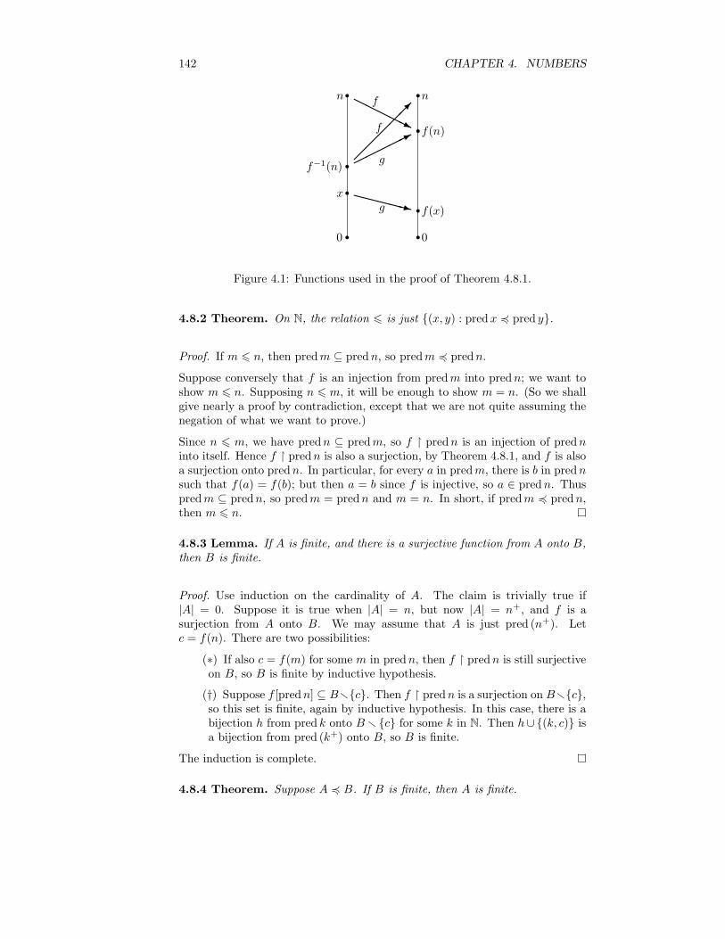
142 CHAPTER 4. NUMBERS
0 0
n n
x
f(x)
f−1(n)
f(n)
r r
r r
r rrr
f
f
g
g¡¡¡¡¡µ
©©©©©*
XXXXXz
HHHHHj
Figure 4.1: Functions used in the proof of Theorem 4.8.1.
4.8.2 Theorem. On N, the relation 6 is just (x, y) : predx 4 pred y.
Proof. If m 6 n, then predm ⊆ predn, so predm 4 predn.
Suppose conversely that f is an injection from predm into predn; we want toshow m 6 n. Supposing n 6 m, it will be enough to show m = n. (So we shallgive nearly a proof by contradiction, except that we are not quite assuming thenegation of what we want to prove.)
Since n 6 m, we have predn ⊆ predm, so f ¹ predn is an injection of predninto itself. Hence f ¹ predn is also a surjection, by Theorem 4.8.1, and f is alsoa surjection onto predn. In particular, for every a in predm, there is b in prednsuch that f(a) = f(b); but then a = b since f is injective, so a ∈ predn. Thuspredm ⊆ predn, so predm = predn and m = n. In short, if predm 4 predn,then m 6 n.
4.8.3 Lemma. If A is finite, and there is a surjective function from A onto B,then B is finite.
Proof. Use induction on the cardinality of A. The claim is trivially true if|A| = 0. Suppose it is true when |A| = n, but now |A| = n+, and f is asurjection from A onto B. We may assume that A is just pred (n+). Letc = f(n). There are two possibilities:
(∗) If also c = f(m) for some m in predn, then f ¹ predn is still surjectiveon B, so B is finite by inductive hypothesis.
(†) Suppose f [predn] ⊆ Brc. Then f ¹ predn is a surjection on Brc,so this set is finite, again by inductive hypothesis. In this case, there is abijection h from pred k onto Br c for some k in N. Then h∪ (k, c) isa bijection from pred (k+) onto B, so B is finite.
The induction is complete.
4.8.4 Theorem. Suppose A 4 B. If B is finite, then A is finite.
4.8. CARDINALITY 143
Proof. It is enough to show that if A ⊆ B, and B is finite, then A is finite. If Ais empty, then |A| = 0. Suppose A contains c. Define f from B to A by:
f(x) =
x, if x ∈ A;c, if x /∈ A.
Then f is surjective, so the claim follows by Lemma 4.8.3.
4.8.5 Theorem. If A is infinite, then N 4 A.
Proof. There is a non-surjective injection s : A → A. Let c ∈ A r s[A]. Then(A, s, c) satisfies Axiom Z and Axiom U. Now let
S = C ∈ P(A) : c ∈ C ∧ s[C] ⊆ C.
Then S contains A itself, so S is non-empty; so we can let B =⋂S. Then
(B, s ¹ B, c) satisfies all three Peano axioms (exercise). By Theorem 4.1.2, thereis an isomorphism from (N,+, 0) to (B, s ¹ B, c); this function is an injectionfrom N to A.
By Theorem 4.8.4, if A 4 B, and A is not finite, then B is not finite. Below weshall show that the non-infinite sets are precisely the infinite sets; but this willrequire a new set-theoretic axiom. Without this, we can still prove:
4.8.6 Theorem. Suppose A 4 B. If A is infinite, then B is infinite.
Proof. Suppose the functions f : A → B and g : A → A are injections. Thenf g f−1 is an injection from f [A] to B. Let C = B r f [A], and let h be theunion (f g f−1) ∪ idC . Then h is an injection from B to itself. If c /∈ g[A],then f(c) /∈ h[B].
By this theorem, we can show that a set A is infinite if we can find an injectivefunction G from N to A. That G is injective means precisely that
G(n+) ∈ Ar G(0), . . . , G(n)
for all n in N. Now, if A is not finite, then in each case the set
Ar G(0), . . . , G(n)
is not empty by Lemma 4.8.3, so there is some hope that the function G exists.Does strong recursion (that is, Corollary 4.7.5) give us such a function G? Itdoes, if there is a function h : P(A) → A such that h(X) /∈ X when X 6= A.However, we have no reason, so far, to assert that such a function exists. Thatfunctions like h exist is a consequence of:
4.8.7 Axiom (Choice). For every set A, there is a function f : P(A)→ A suchthat f(C) ∈ C whenever C 6= 0.
A function f as in the axiom is called a choice-function.
4.8.8 Theorem. Every set is either finite or infinite.
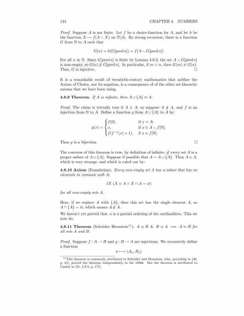
144 CHAPTER 4. NUMBERS
Proof. Suppose A is not finite. Let f be a choice-function for A, and let h bethe function X 7→ f(A rX) on P(A). By strong recursion, there is a functionG from N to A such that
G(n) = h(G[predn]) = f(ArG[predn])
For all n in N. Since G[predn] is finite by Lemma 4.8.3, the set ArG[predn]is non-empty, so G(n) /∈ G[predn]. In particular, if m < n, then G(m) 6= G(n).Thus, G is injective.
It is a remarkable result of twentieth-century mathematics that neither theAxiom of Choice, nor its negation, is a consequence of of the other set-theoreticaxioms that we have been using.
4.8.9 Theorem. If A is infinite, then A ∪ A ≈ A.
Proof. The claim is trivially true if A ∈ A; so suppose A /∈ A, and f is aninjection from N to A. Define a function g from A ∪ A to A by:
g(x) =
f(0), if x = A;
x, if x ∈ Ar f [N];
f(f−1(x) + 1), if x ∈ f [N].
Then g is a bijection.
The converse of this theorem is true, by definition of infinite, if every set A is aproper subset of A ∪ A. Suppose if possible that A = A ∪ A. Then A ∈ A,which is very strange, and which is ruled out by:
4.8.10 Axiom (Foundation). Every non-empty set A has a subset that has noelements in common with A:
∃X (X ∈ A ∧ X ∩A = ∅)
for all non-empty sets A.
Here, if we replace A with A, then this set has the single element A, soA ∩ A = ∅, which means A /∈ A.We haven’t yet proved that 4 is a partial ordering of the cardinalities. This wenow do.
4.8.11 Theorem (Schroder–Bernstein11). A 4 B & B 4 A =⇒ A ≈ B forall sets A and B.
Proof. Suppose f : A→ B and g : B → A are injections. We recursively definea function
n 7−→ (An, Bn)
11This theorem is commonly attributed to Schroder and Bernstein, who, according to [40,p. 81], proved the theorem independently in the 1890s. But the theorem is attributed toCantor in [31, § 8.3, p. 171].
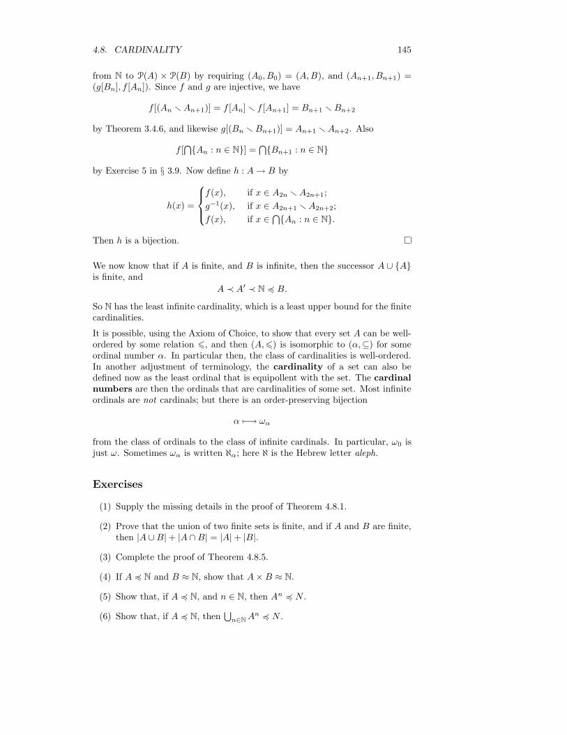
4.8. CARDINALITY 145
from N to P(A) × P(B) by requiring (A0, B0) = (A,B), and (An+1, Bn+1) =(g[Bn], f [An]). Since f and g are injective, we have
f [(An rAn+1)] = f [An] r f [An+1] = Bn+1 rBn+2
by Theorem 3.4.6, and likewise g[(Bn rBn+1)] = An+1 rAn+2. Also
f [⋂An : n ∈ N] = ⋂Bn+1 : n ∈ N
by Exercise 5 in § 3.9. Now define h : A→ B by
h(x) =
f(x), if x ∈ A2n rA2n+1;
g−1(x), if x ∈ A2n+1 rA2n+2;
f(x), if x ∈ ⋂An : n ∈ N.
Then h is a bijection.
We now know that if A is finite, and B is infinite, then the successor A ∪ Ais finite, and
A ≺ A′ ≺ N 4 B.
So N has the least infinite cardinality, which is a least upper bound for the finitecardinalities.
It is possible, using the Axiom of Choice, to show that every set A can be well-ordered by some relation 6, and then (A,6) is isomorphic to (α,⊆) for someordinal number α. In particular then, the class of cardinalities is well-ordered.In another adjustment of terminology, the cardinality of a set can also bedefined now as the least ordinal that is equipollent with the set. The cardinalnumbers are then the ordinals that are cardinalities of some set. Most infiniteordinals are not cardinals; but there is an order-preserving bijection
α 7−→ ωα
from the class of ordinals to the class of infinite cardinals. In particular, ω0 isjust ω. Sometimes ωα is written ℵα; here ℵ is the Hebrew letter aleph.
Exercises
(1) Supply the missing details in the proof of Theorem 4.8.1.
(2) Prove that the union of two finite sets is finite, and if A and B are finite,then |A ∪B|+ |A ∩B| = |A|+ |B|.
(3) Complete the proof of Theorem 4.8.5.
(4) If A 4 N and B ≈ N, show that A×B ≈ N.
(5) Show that, if A 4 N, and n ∈ N, then An 4 N .
(6) Show that, if A 4 N, then⋃n∈N
An 4 N .
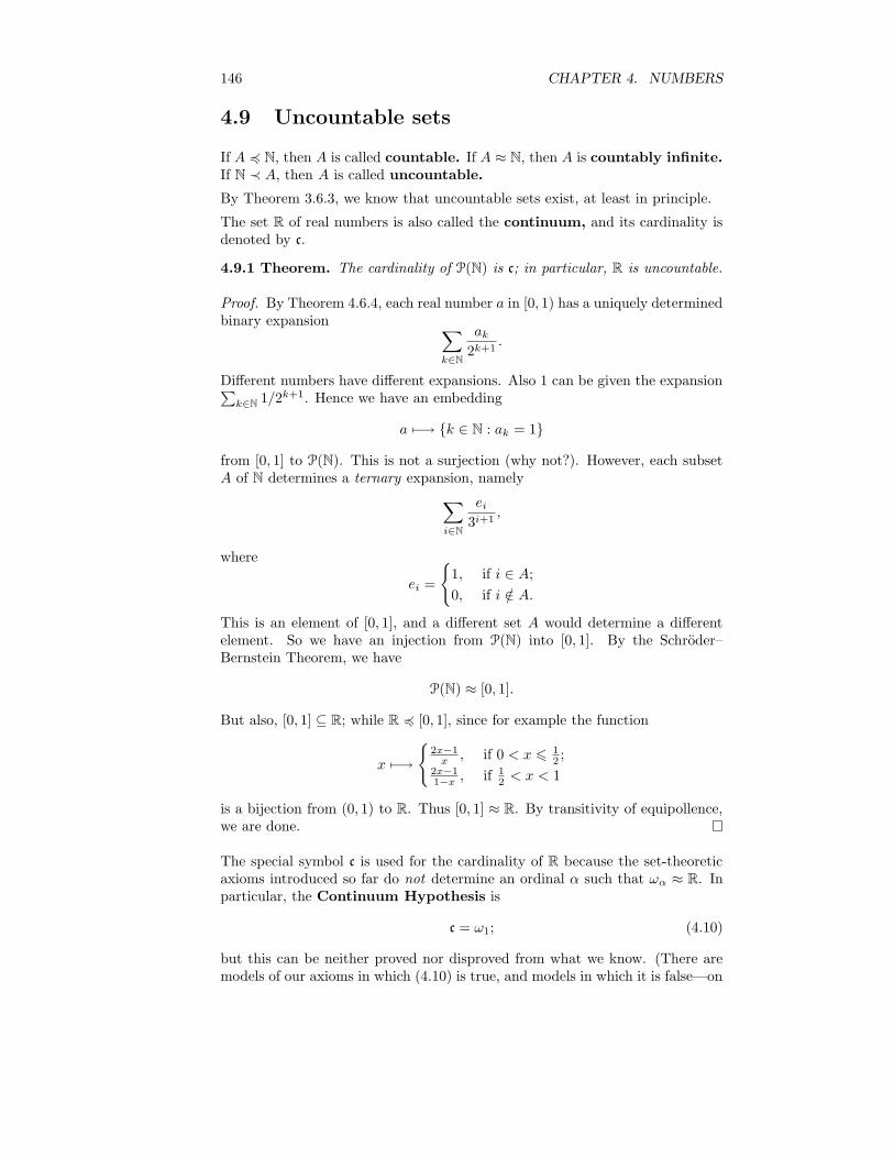
146 CHAPTER 4. NUMBERS
4.9 Uncountable sets
If A 4 N, then A is called countable. If A ≈ N, then A is countably infinite.If N ≺ A, then A is called uncountable.
By Theorem 3.6.3, we know that uncountable sets exist, at least in principle.
The set R of real numbers is also called the continuum, and its cardinality isdenoted by c.
4.9.1 Theorem. The cardinality of P(N) is c; in particular, R is uncountable.
Proof. By Theorem 4.6.4, each real number a in [0, 1) has a uniquely determinedbinary expansion ∑
k∈N
ak2k+1
.
Different numbers have different expansions. Also 1 can be given the expansion∑k∈N
1/2k+1. Hence we have an embedding
a 7−→ k ∈ N : ak = 1
from [0, 1] to P(N). This is not a surjection (why not?). However, each subsetA of N determines a ternary expansion, namely
∑
i∈N
ei3i+1
,
where
ei =
1, if i ∈ A;0, if i /∈ A.
This is an element of [0, 1], and a different set A would determine a differentelement. So we have an injection from P(N) into [0, 1]. By the Schroder–Bernstein Theorem, we have
P(N) ≈ [0, 1].
But also, [0, 1] ⊆ R; while R 4 [0, 1], since for example the function
x 7−→
2x−1x, if 0 < x 6 1
2 ;2x−11−x , if 1
2 < x < 1
is a bijection from (0, 1) to R. Thus [0, 1] ≈ R. By transitivity of equipollence,we are done.
The special symbol c is used for the cardinality of R because the set-theoreticaxioms introduced so far do not determine an ordinal α such that ωα ≈ R. Inparticular, the Continuum Hypothesis is
c = ω1; (4.10)
but this can be neither proved nor disproved from what we know. (There aremodels of our axioms in which (4.10) is true, and models in which it is false—on

4.9. UNCOUNTABLE SETS 147
the assumption that there are models of our axioms at all, and this is somethingthat we cannot prove either.)
If we only want to show N ≺ R, we can use the following diagonal argument.Suppose f is a function from N into [0, 1]. If n ∈ N, write
f(n) =∑
i∈N
an,i10i+1
,
where an,i ∈ 10. Now define
bi =
5, if ai,i 6= 5;
0, if ai,i = 5.
Then f(n) is never equal to∑
i∈Nbi/10
i+1; so f is not surjective.
Exercises
(1) Show that R is equipollent with the set of functions from N to N.
(2) Show that R× R ≈ R.
(3) A real number α is algebraic if there is no positive integer n for whichthere is an n-tuple ~a of rational numbers such that
∑
k<n
akαk + αn = 0.
A real number that is not algebraic is transcendental. Show that thereare uncountably many transcendental numbers.

Appendix A
Aristotle’s Analytics
Below is a translation from the first few pages of the Aristotelian work called thePrior Analytics. Like all of Aristotle’s extant works, the text appears to consistof students’ lecture notes; perhaps these notes were never edited by Aristotlehimself.
I only want to observe three features of the text:
(∗) the absence of any special notation;
(†) the definition of proposition;
(‡) the use of proofs.
The translation here is mine, from the text in [2]. Some of the wording isfrom the English translation by Tredennick that accompanies that text, butthere are deviations. For example, where I have ‘proposition’, Tredennick has‘premiss’. The typography is entirely my own, based on the conception of thetext as lecture-notes; the Greek text indicates no special line-breaks. Likewise,my English is highly abbreviated and ‘telegraphic’, as is the original Greek.
Here then is Aristotle:
First, to say what our study (σκέψιc) is about and of :
(∗) it is about demonstration (πόδειξιc), and
(†) it is of demonstrative science (âπιστήµη ποδεικτικη).
Next, to define:
(∗) proposition (πρότασιc), term (íροc), and syllogism (συllογισµόc), and
(†) which kinds [of syllogism] are complete (τέlειοc) and incomplete (τεlήc).
After these:
(‡) what it is for one thing to be or not to be wholly (τä âν ílú εÚναι « µεÚναι) in another, and
(§) what we mean by being predicated (κατηγορεισθαι) of all or of none.
A proposition is a statement affirming (καταφατικόc) or denying (ποφατικόc)something of something. It is universal (καθόlου), particular (âν µερει), orindefinite (διόριστοc).
148

149
(∗) By universal, I mean applying (Íπάρχειν) to all or none;
(†) by particular, applying to some, or not to some, or not to all;
(‡) by indefinite, applying or not applying, without reference to whole orpart, as in ‘The same science studies contraries’ or ‘Pleasure is not good.’
[I skip some further discussion of propositions.]
A term is what a proposition is divided into, namely
(∗) that which is predicated, and
(†) that of which it is predicated,
[a form of] to be or not to be being added or removed.
A syllogism is a ‘piece of language’ (lόγοc) in which, some things being as-sumed (τεθέντων τινων), because of these (τÄ ταυτα εÚναι), something differentfrom what was laid down (τα κειµένα) necessarily follows. By saying:
(∗) ‘because of these,’ I mean it follows through these (δι ταυτα);
(†) ‘it follows through these,’ no additional term is needed for the necessityto come about.
I call a syllogism:
(∗) complete, if it needs nothing else, apart from what it [already] contains,for the necessary [conclusion] to be evident;
(†) incomplete, if it needs one or more [propositions] not included amongthe [given] propositions, although they are necessary through the termsthat have been laid down.
These are the same:
(∗) for this to be wholly in that ;
(†) for that to be predicated of all of this.
We say that [that is] predicated of all [of this] when nothing of this can be takenof which that cannot be said. Similarly if [that ] is predicated of none [of this].
Now, every proposition is
(∗) an application (Íπάρχειν), or
(†) a necessary (âξ νάνκηc) application, or
(‡) a potential (του âνδέχεσθαι) application.
Of these,
(∗) some are affirmative (καταφατικόc),
(†) some negative (ποφατικόc),
according to each application.
Again, of the affirmative and negative, some are universal, some particular,some indefinite.
A universal
(∗) negative (στερητικόc) application is necessarily convertible (ντιστρέφειν)in terms; for example, if no pleasure is a good thing, then no good thingis a pleasure;
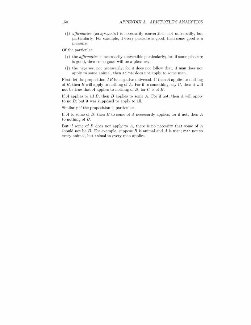
150 APPENDIX A. ARISTOTLE’S ANALYTICS
(†) affirmative (κατηγορικόc) is necessarily convertible, not universally, butparticularly. For example, if every pleasure is good, then some good is apleasure.
Of the particular:
(∗) the affirmative is necessarily convertible particularly; for, if some pleasureis good, then some good will be a pleasure;
(†) the negative, not necessarily; for it does not follow that, if man does notapply to some animal, then animal does not apply to some man.
First, let the proposition AB be negative universal. If then A applies to nothingof B, then B will apply to nothing of A. For if to something, say C, then it willnot be true that A applies to nothing of B, for C is of B.
If A applies to all B, then B applies to some A. For if not, then A will applyto no B; but it was supposed to apply to all.
Similarly if the proposition is particular:
If A to some of B, then B to some of A necessarily applies; for if not, then Ato nothing of B.
But if some of B does not apply to A, there is no necessity that some of Ashould not be B. For example, suppose B is animal and A is man; man not toevery animal, but animal to every man applies.

Bibliography
[1] Aristoteles. Metafizik. Sosyal Yayınlar, Cagaloglu–Istanbul, 1996. Secondprinting. Turkish translation by Ahmet Arslan.
[2] Aristotle. Categories, On Interpretation, and Prior Analytics, volume 325of Loeb Classical Library. Harvard University Press and William Heine-mann Ltd, Cambridge, Massachusetts and London, 1973. Translated by H.P. Cooke and H. Tredennick.
[3] Aristotle. The Metaphysics, Books I–IX, volume XVII of Loeb ClassicalLibrary. Harvard University Press, Cambridge, Massachusetts, USA, 1980.With an English translation by Hugh Tredennick. First printed 1933.
[4] George Boole. Collected Logical Works. Volume II: The Laws of Thought.The Open Court Publishing Company, Chicago and London, 1940. Firstpublished 1854. With a note by Philip E.B. Jourdain.
[5] Stanley N. Burris. Logic for Mathematics and Computer Science. PrenticeHall, Upper Saddle River, New Jersey, USA, 1998.
[6] C. C. Chang and H. J. Keisler. Model theory. North-Holland Publishing Co.,Amsterdam, 1973. Studies in Logic and the Foundations of Mathematics,Vol. 73.
[7] Alonzo Church. Introduction to mathematical logic. Vol. I. Princeton Uni-versity Press, Princeton, N. J., 1956.
[8] R. G. Collingwood. An Autobiography. Clarendon Press, c. 1938. Reprinted2002.
[9] Richard Dedekind. Essays on the theory of numbers. I:Continuity and irra-tional numbers. II:The nature and meaning of numbers. Dover PublicationsInc., New York, 1963.
[10] Rene Descartes. The Geometry of Rene Descartes. Dover Publications,Inc., New York, 1954. Translated from the French and Latin by DavidEugene Smith and Marcia L. Latham, with a facsimile of the first edition.
[11] John Donne. The Complete Poetry and Selected Prose of John Donne. TheModern Library, New York, 1952. Edited with an introduction by CharlesM. Coffin.
151
152 BIBLIOGRAPHY
[12] Lou van den Dries and Yiannis N. Moschovakis. Is the Euclidean algo-rithm optimal among its peers? Bulletin of Symbolic Logic, 10(3):390–418,September 2004.
[13] Susanna S. Epp. Discrete Mathematics with Applications. PWS PublishingCompany, Boston, Massachusetts, USA, 1995. 2nd edition.
[14] Euclid. The thirteen books of Euclid’s Elements translated from the text ofHeiberg. Vol. I: Introduction and Books I, II. Vol. II: Books III–IX. Vol.III: Books X–XIII and Appendix. Dover Publications Inc., New York, 1956.Translated with introduction and commentary by Thomas L. Heath, 2nded.
[15] Anita Burdman Feferman and Solomon Feferman. Alfred Tarski: life andlogic. Cambridge University Press, Cambridge, 2004.
[16] Paul R. Halmos. Naive set theory. Springer-Verlag, New York, 1974.Reprint of the 1960 edition, Undergraduate Texts in Mathematics.
[17] G. H. Hardy. A mathematician’s apology. Cambridge University Press,Cambridge, 1992. With a foreword by C. P. Snow, Reprint of the 1967edition.
[18] Richard D. Heffner. A Documentary History of the United States. NewAmerican Library, New York, 3rd edition, 1976. Expanded and RevisedBicentennial Edition.
[19] Leon Henkin. The completeness of the first-order functional calculus. J.Symbolic Logic, 14:159–166, 1949.
[20] Wilfrid Hodges. Model theory, volume 42 of Encyclopedia of Mathematicsand its Applications. Cambridge University Press, Cambridge, 1993.
[21] Homer C House and Susan Emolyn Harman. Descriptive English Grammar.Prentice-Hall, Englewood Cliffs, N.J., USA, second edition, 1950. Revisedby Susan Emolyn Harman. Twelfth printing, 1962.
[22] Jacob Klein. Greek mathematical thought and the origin of algebra. DoverPublications Inc., New York, 1992. Translated from the German and withnotes by Eva Brann, Reprint of the 1968 English translation.
[23] Morris Kline. Mathematical thought from ancient to modern times. OxfordUniversity Press, New York, 1972.
[24] Donald E. Knuth. The TEXbook, volume A of Computers & Typesetting.Addison Wesley Publishing Company, Reading, Massachusetts, USA, June1986. Seventh printing.
[25] Edmund Landau. Foundations of Analysis. The Arithmetic of Whole, Ra-tional, Irrational and Complex Numbers. Chelsea Publishing Company,New York, N.Y., 1951. Translated by F. Steinhardt.
[26] Azriel Levy. Basic set theory. Dover Publications Inc., Mineola, NY, 2002.Reprint of the 1979 original [Springer, Berlin; MR0533962 (80k:04001)].

BIBLIOGRAPHY 153
[27] David Marker. Model theory, volume 217 ofGraduate Texts in Mathematics.Springer-Verlag, New York, 2002. An introduction.
[28] Murray et al., editors. The Compact Edition of the Oxford English Dictio-nary. Oxford University Press, 1973.
[29] Ali Nesin. Onermeler Mantıgı. Istanbul Bilgi Universitesi Yayınları, 2001.
[30] Filiz Oktem. Uygulamalı Latin Dili. Sosyal Yayınlar, Eylul 1996.
[31] Bruno Poizat. A course in model theory. Universitext. Springer-Verlag,New York, 2000. An introduction to contemporary mathematical logic,Translated from the French by Moses Klein and revised by the author.
[32] Emil L. Post. Introduction to a general theory of elementary propositions.Amer. J. Math., 43(3):163–185, July 1921.
[33] Paul Reps and Nyogen Senzaki, editors. Zen Flesh, Zen Bones. Shambala,Boston, 1994. A Collection of Zen and Pre-Zen Writings.
[34] Kenneth A. Ross and Charles R.B. Wright. Discrete mathematics. 4th ed.Upper Saddle River, NJ: Prentice Hall. xiv, 684 p. $ 113.04 , 1999.
[35] Philipp Rothmaler. Introduction to model theory, volume 15 of Algebra,Logic and Applications. Gordon and Breach Science Publishers, Amster-dam, 2000. Prepared by Frank Reitmaier, Translated and revised from the1995 German original by the author.
[36] Joseph J. Rotman. A first course in abstract algebra. Prentice Hall Inc.,Upper Saddle River, NJ, 2nd edition, 2000.
[37] Joseph H. Silverman. The arithmetic of elliptic curves, volume 106 ofGraduate Texts in Mathematics. Springer-Verlag, New York, 1986.
[38] Paul Simon and Art Garfunkel. Simon and Garfunkel. Oyku Yayıncılık,Sultanahmet, Istanbul, 1987. Words and music of songs of Paul Simon andArt Garfunkel; Turkish translation by Devrim Eker.
[39] Michael Spivak. Calculus. 2nd ed. Berkeley, California: Publish Perish,Inc. XIII, 647 p. , 1980.
[40] Robert R. Stoll. Set theory and logic. Dover Publications Inc., New York,1979. Corrected reprint of the 1963 edition.
[41] Patrick Suppes. Axiomatic set theory. Dover Publications Inc., New York,1972. Unabridged and corrected republication of the 1960 original with anew preface and a new section (8.4).
[42] Alfred Tarski. Truth and proof. Scientific American, pages 63–77, 1969.
[43] Alfred Tarski. Introduction to Logic and to the Methodology of DeductiveSciences. Dover, 1995. An unabridged republication of the 9th printing,1961, of the 1946 second, revised edition of the work originally publishedby Oxford University Press, New York, in 1941.

154 BIBLIOGRAPHY
[44] Ivor Thomas, editor. Selections illustrating the history of Greek mathemat-ics. Vol. I. From Thales to Euclid. Harvard University Press, Cambridge,Mass., 1951. With an English translation by the editor.
[45] Ivor Thomas, editor. Selections illustrating the history of Greek mathe-matics. Vol. II. From Aristarchus to Pappus. Harvard University Press,Cambridge, Mass, 1951. With an English translation by the editor.
[46] Della Thompson, editor. The Concise Oxford Dictionary of Current En-glish. Clarendon Press, Oxford, ninth edition, 1995.
[47] Jean van Heijenoort. From Frege to Godel. A source book in mathematicallogic, 1879–1931. Harvard University Press, Cambridge, Mass., 1967.
[48] Jean van Heijenoort, editor. Frege and Godel. Two fundamental texts inmathematical logic. Harvard University Press, Cambridge, Mass., 1970.
[49] Andre Weil. Number theory. Birkhauser Boston Inc., Boston, MA, 1984.An approach through history, From Hammurapi to Legendre.
[50] Howard Zinn. A People’s History of the United States: 1492–Present.Harper Collins, New York, 2nd edition, 1995.

Symbols
= 7a, b, c 8d ∈ C 8d /∈ C 8
∅ 8C ⊆ D 8C 6⊆ D 9A = B 9A ⊂ B 9A 6= B 9x : Px 9U 10
A ∪B 10A′ 100 10
n+ 1 11m 6 n 11n− 1 12
0, . . . , n− 1 12N 12n+ 12n+ 1 12−1 13−n 13Z 13
x+ y 13−x 13x · y 13xy 13( ) 15
x2 17x < y 17y/x 18Q 18x | y 18|a| 22
gcd(a, b) 23R 23√2 23
a : b :: c : d 24p(x) 26x¯ y 27x⊕ y 27xª y 27x t y 27P ∧ Q 29P = Q 29¬P 29P ∨Q 29P → Q 30P ↔ Q 30A & B 33A =⇒ B 33A ⇐⇒ B 34
∃x 37∀x 37Ac 37² 39
F 41F (P0, . . . , Pn−1) 41
155
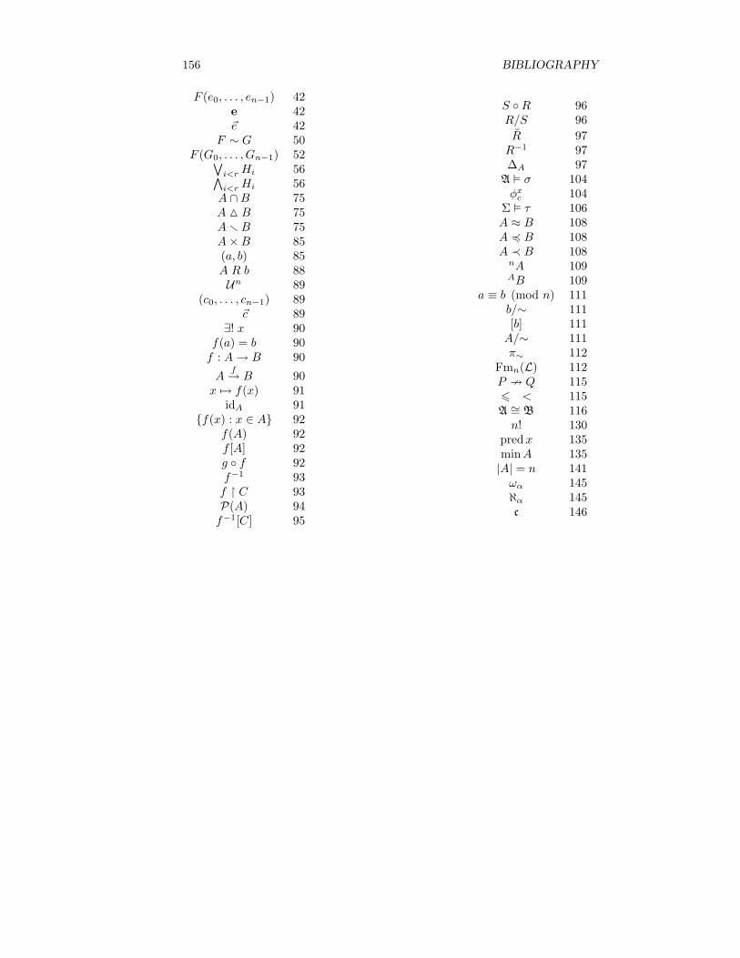
156 BIBLIOGRAPHY
F (e0, . . . , en−1) 42e 42~e 42
F ∼ G 50F (G0, . . . , Gn−1) 52∨
i<rHi 56∧i<rHi 56A ∩B 75A M B 75ArB 75A×B 85(a, b) 85A R b 88Un 89
(c0, . . . , cn−1) 89~c 89
∃! x 90f(a) = b 90f : A→ B 90
Af→ B 90
x 7→ f(x) 91idA 91
f(x) : x ∈ A 92f(A) 92f [A] 92g f 92f−1 93f ¹ C 93P(A) 94f−1[C] 95
S R 96R/S 96
R 97R−1 97∆A 97
A ² σ 104φxc 104
Σ ² τ 106A ≈ B 108A 4 B 108A ≺ B 108nA 109AB 109
a ≡ b (mod n) 111b/∼ 111[b] 111A/∼ 111π∼ 112
Fmn(L) 112P 9 Q 1156 < 115A ∼= B 116n! 130
predx 135minA 135|A| = n 141ωα 145ℵα 145c 146

Index
absolute value, 22Absorption Laws, 63, 80addend, 13addition, 13, 70, 125additive
— inverse, 13— inversion, 13
adequacy, 58adequate, 58adjective, 35
article, 35demonstrative —, 35descriptive —, 35determiner, 36existential —, 36logical —, 36negative —, 36quantitative —, 35universal —, 36
admits— definition by recursion, 124— definition by strong recursion,
135— proof by induction, 124— proof by strong induction, 135
adversative conjunction, 32affirmation of the consequent, 71aleph, 145algebraic, 147algorithm
Euclidean —, 22, 23alternating
— subtraction, 25alternative conjunction, 32antecedent, 33anthyphaeresis, 25anti-symmetric, 113architect, 32
—ure, 114
architecture, viargument, 46arithmetic
— inequality, 98— term, 98— formula, 16— identity, 16— inequality, 18— term, 2, 14
arity, 46binary, 41, 46n-ary, 41nullary, 41, 46singulary, 41, 46ternary, 41unary, 41
articledefinite —, 35indefinite —, 35
assignmenttruth-—, 42
associated, 115associative, 52, 126, 127associativity, 61
A— Lemma, 53Law of A—, 79
atomic— formula, 100
atomic formula, 98axiom, iii, 2, 3, 69, 106
—atizes, 106—-scheme, 106A— of Existence of N, 120A— I, 121A— of Extension, 77A— of Separation, 119A— of Choice, 93, 143A— of Comprehension, 10A— of Extension, 9
157

158 INDEX
A— of Foundation, 144A— of Induction, 121A— of Infinity, 121A— of Separation, 10, 76A— of the Power-set, 94A— U, 120A— Z, 120Peano A—s, 121
base step, 11, 123biconditional, 30, 34bijection, 91bijective, 91binary, 41, 46
— relation, 88bind, 103binomial
— coefficient, 126B— Theorem, 133
Boolean— combination, 76— connective, 26, 29— operation, 75— term, 30
bound occurrence of variable, 102, 104
calculusinfinitesimal —, 38, 91infinitesimal —, 1propositional —, 1, 23
cancellation, 126cardinal number, 145cardinality, 113, 141, 145Cartesian product, iii, 85cases, 70characteristic function, 136characteristic function, 110choice
—-function, 143Axiom of C—, 93, 143
class, 7equivalence-—, 111
closed formula, 31co-domain, 89, 90coefficient
binomial —, 126collective noun, 7combination
Boolean —, 76commutative, 126, 127
commutativity, 61Law of C—, 79
commutes, 112, 123compactness theorem, 107complement, 37, 75complete theory, 106completeness, 69, 107compose, 8composite, 18composition, 14, 96comprehension
Axiom of C—, 10comprises, 8condition
necessary —, 112sufficient —, 112
conditional, 30, 33congruence
— modulo n, 111, 125conjunction, 29, 32, 33
adversative —, 32alternative —, 32coordinating —, 32cumulative —, 32disjunctive —, 32subordinating —, 32transitional —, 32
conjunctive normal form, 57connective
Boolean —, 26, 29Schroder —, 60Sheffer stroke, 61
consequencelogical —, 64, 106
consequent, 33affirmation of the —, 71
consistent, 124consists of, 8constant, 15, 30, 98, 99
— term, 101literal —, 15numeral —, 15
constituentnormal disjunctive —, 55
constructive dilemma, 70contains, 8context, 2, 104contingency, 51continued fraction, 25continuous, 38, 91

INDEX 159
continuum, 146C— Hypothesis, 146
contradiction, 51, 70Law of C—, 6proof by —, 20, 142
contraposition, 34, 71, 123contrapositive, 35, 122, 139converse, 35, 77, 80, 82, 93, 96conversion, 34coordinating conjunction, 32Corinthian order, vicorollary, 7correspondence
one-to-one —, 91countable, 107, 146countably infinite, iv, 146cumulative conjunction, 32
dashswung —, 50
De Morgan’s Laws, 61, 79decreasing
strictly —, 21deducible, 65deduction, iii, 65, 69
D— Theorem, 71recognizable —, 67
definedwell-—, 112
defines, 85definite article, 35definition, 61
— by induction, 124— by recursion, 124admits — by recursion, 124admits — by strong recursion, 135inductive —, 10, 15, 124recursive —, 124
demonstrative adjective, 35derivable, 69descent
infinite —, 67infinite —, 20, 48, 72
descriptive adjective, 35detachment, 69, 70
D— Lemma, 65determiner, 36diagram
commutative —, 112, 123difference, 14, 75
symmetric —, 75dilemma
constructive —, 70Diophantine equation, 98Diophantine equation, 16disjoint, 75disjunction, 33
exclusive —, 29inclusive —, 29
disjunctive— normal form, 55, 56— syllogism, 70normal — constituent, 55
disjunctive conjunction, 32distributes, 127distributive, 17, 127distributivity, 61
Law of D—, 79self-— of implication, 71
divides, 18divisor, 18
proper —, 133domain, 89, 90, 100
co-—, 89, 90Doric order, 114double
— negation, 61—t, 13—ton, 86
element, 7greatest element, 139least —, 135minimal —, 135
elimination of quantifiers, 107embedding, 91empty set, 8equal, 9equality, 97
sign of —, 7, 30, 98equation
Diophantine —, 16, 98member of an —, 7
equipollence, 111equipollent, iv, 108equipotent, 108equivalence, 34
—-class, 16, 76, 111—-relation, iv, 110, 116material —, 30

160 INDEX
equivalent, 50, 87T -equivalent, 107truth-—, 50
Euclidean algorithm, 22, 23even number, 20excluded
Law of the E— Middle, 6exclusive
— disjunction, 29existential
— adjective, 36— quantifier, 37
extensionAxiom of E—, 9, 77
factor, 13, 112—ial, 130
false, 2, 104field
ordered —, 107final
— segment, 47finite, 141first
—-order formula, 101—-order logic, iv, 98, 101
formal— proof, iii, 28, 51, 65, 69—ly provable, 65, 69
formula, 76, 98, 101arithmetic —, 16atomic —, 98, 100∈-—, 74first-order formula, 101n-ary —, 103propositional —, 30sentence, 104set-theoretic —, 74sub-—, 43
foundation, i, 4Axiom of F—, 144
fractioncontinued —, 25
free— occurrence of variable, 104— variable, 102
from, 90full truth-table, 44function, iv, 13, 90
—-symbol, 98, 99
characteristic —, 110, 136choice-—, 143factor, 112homomorphism, 116interpretation-—, 100isomorphism, 116projection, 102, 111quotient-map, 111
Godel, 106, 107—’s Incompleteness Theorem, 106
goodwell-ordered, 135
grammar, 6, 32greatest element, 139
Henkin, 107homomorphism, 116, 124hypothesis, 65, 69
Continuum H—, 146inductive —, 11, 123strong inductive —, 138
hypothetical syllogism, 70
idempotent, 26identity, 91, 127
arithmetic —, 16immediate predecessor, 12implication, 33
material —, 30, 34self-distributivity of —, 71tautological —, 81
in, 8included in, 8includes, 8inclusion
tautological —, 81inclusive disjunction, 29incomplete
Godel’s I—ness Theorem, 106indefinite article, 35individual variable, 74, 100induction, 11
— on x, 126admits proof by —, 124admits proof by strong —, 135Axiom of I—, 121definition by —, 124proof by —, 2, 11, 15
inductive
INDEX 161
— hypothesis, 123— definition, 10, 15, 124— hypothesis, 11— step, 11—step, 123strong — hypothesis, 138
inequality, 18arithmetic —, 98
inequation, 18inference
rule of —, 69infinitary
— intersection, 118— union, 118
infinite, 8, 122— descent, 20, 48, 67, 72countably —, iv, 146uncountable, iv, 146
infinitesimal— calculus, 1, 38, 91
infinityAxiom of I—, 121
infix notation, 49initial segment, 47injection, 91injective, 91integer, 13, 18, 128
negative —, 13, 18positive —, 18
interpretation, 85, 99—-function, 100
intersection, 75infinitary —, 118
inverse, 93additive —, 13
inversionadditive —, 13
invertible, 93irrational, 23irreflexive, 113is to. . . as . . . is to . . . , 24isomorphic, 116isomorphism, 116
juxtaposition, 13
largerstrictly —, 108
lawAbsorption L—s, 63, 80
De Morgan’s L—s, 61, 79L— of Associativity, 61, 79L— of Commutativity, 61, 79L— of Contradiction, 6L— of Distributivity, 61, 79L— of the Excluded Middle, 6
least element, 135lemma, 7
Associativity L—, 53Detachment L—, 65
limit, 139linear order, 115list, 89literal constant, 15logic, 1
—al adjective, 36—al consequence, 64, 106a propositional —, 58first-order —, iv, 98first-order logic, 101mathematical —, 2predicate —, iii, 35propositional —, iii, 99second-order —, 107symbolic —, 1
ÃLukasiewicz, 49
Mal’tsev, 107map, 90
quotient-—, 111material
— equivalence, 30— implication, 30, 34— non-equivalence, 29
mathematical logic, 2meaning, 2member
— of a class, 7— of an equation, 7
mention, vmetaphysics, 4method
— of infinite descent, 67— of infinite descent, 20, 48— of simplification, 51truth-table —, 50
middleLaw of the Excluded M—, 6
minimal element, 135minuend, 14
162 INDEX
minus, 13model, 32, 35, 74, 106
—-theory, 99modifies, 35modulo
congruence — n, 111, 125modus
M— Ponens, 69M— Tollens, 70
multiplication, 13, 126
name, 31, 41n-ary, 41
— formula, 103— function-symbol, 99— operation, 91— predicate, 99— relation-symbol, 99binary, 41, 46nullary, 41, 46singulary, 41, 46ternary, 41unary, 41
natural— number, iv, 2, 8, 10von-Neumann — number, 11
necessary condition, 112negation, 29, 33
double —, 61negative, 13
— integer, 18— adjective, 36— integer, 13
new variable, 62n-factorial, 130non-equivalence
material —, 29non-negative integer, 18normal
— disjunctive constituent, 55conjunctive — form, 57disjunctive — form, 55, 56
notationinfix —, 49ÃLukasiewicz —, 49Polish —, 49, 98, 100reverse Polish —, 49
nouncollective —, 7
n-tuple, 42, 109
nullary, 41, 46— formula, 104— term, 101
number— of times, 22algebraic —, 147cardinal —, 145composite —, 18even —, 20integer, iii, 13irrational —, 23natural —, iv, 2, 8, 10negative integer, 13non-Neumann natural —, 11odd —, 20ordinal —, 140positive —, 13prime —, 18rational —, 18, 112, 129real —, iv, 23transcendental —, 147von-Neumann natural —, 94whole —, 13
numeral, 15
occurrencebound — of variable, 104free — of variable, 104
odd number, 20on, 90
—to, 91one
—-to-—, 91—-to-— correspondence, 91
operation, 13addition, 13, 125additive inversion, 13Boolean —, 75multiplication, 13, 126n-ary, 91order of —s, 16successor-—, 139
order— of operations, 16—ed field, 107—ed n-tuple, 89—ed pair, 85—ing, iv—-preserving, 116Corinthian —, vi
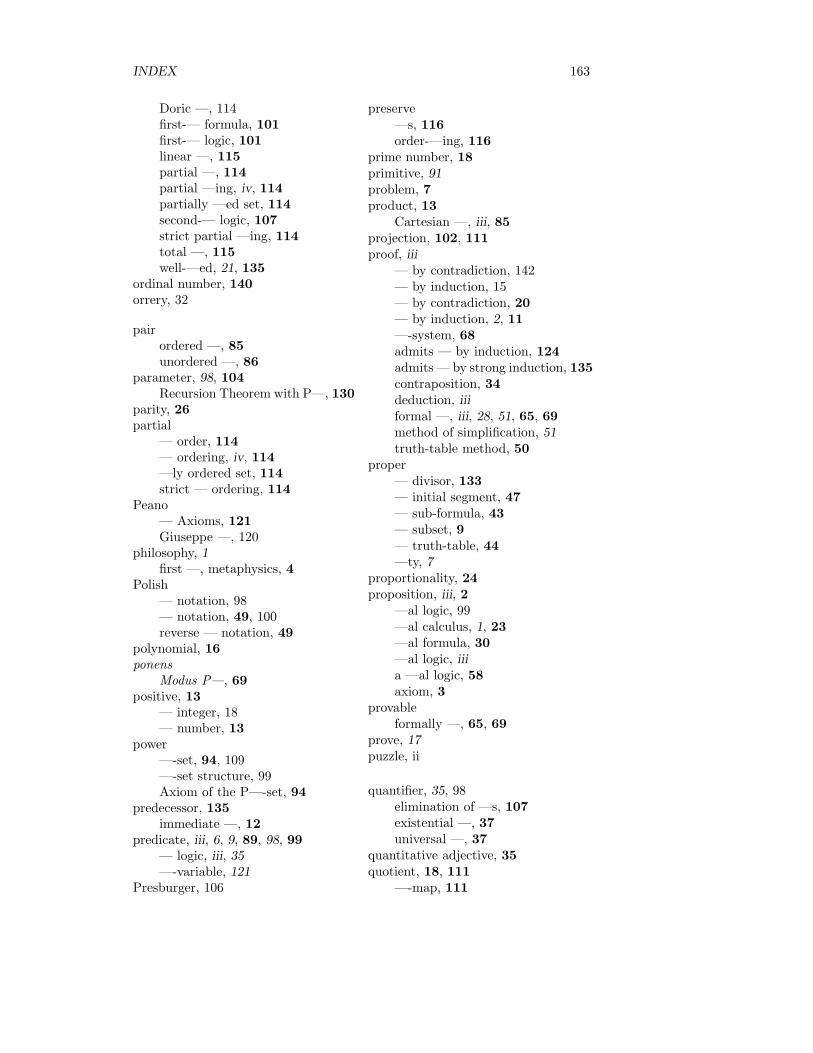
INDEX 163
Doric —, 114first-— formula, 101first-— logic, 101linear —, 115partial —, 114partial —ing, iv, 114partially —ed set, 114second-— logic, 107strict partial —ing, 114total —, 115well-—ed, 21, 135
ordinal number, 140orrery, 32
pairordered —, 85unordered —, 86
parameter, 98, 104Recursion Theorem with P—, 130
parity, 26partial
— order, 114— ordering, iv, 114—ly ordered set, 114strict — ordering, 114
Peano— Axioms, 121Giuseppe —, 120
philosophy, 1first —, metaphysics, 4
Polish— notation, 98— notation, 49, 100reverse — notation, 49
polynomial, 16ponens
Modus P—, 69positive, 13
— integer, 18— number, 13
power—-set, 94, 109—-set structure, 99Axiom of the P—-set, 94
predecessor, 135immediate —, 12
predicate, iii, 6, 9, 89, 98, 99— logic, iii, 35—-variable, 121
Presburger, 106
preserve—s, 116order-—ing, 116
prime number, 18primitive, 91problem, 7product, 13
Cartesian —, iii, 85projection, 102, 111proof, iii
— by contradiction, 142— by induction, 15— by contradiction, 20— by induction, 2, 11—-system, 68admits — by induction, 124admits — by strong induction, 135contraposition, 34deduction, iiiformal —, iii, 28, 51, 65, 69method of simplification, 51truth-table method, 50
proper— divisor, 133— initial segment, 47— sub-formula, 43— subset, 9— truth-table, 44—ty, 7
proportionality, 24proposition, iii, 2
—al logic, 99—al calculus, 1, 23—al formula, 30—al logic, iiia —al logic, 58axiom, 3
provableformally —, 65, 69
prove, 17puzzle, ii
quantifier, 35, 98elimination of —s, 107existential —, 37universal —, 37
quantitative adjective, 35quotient, 18, 111
—-map, 111
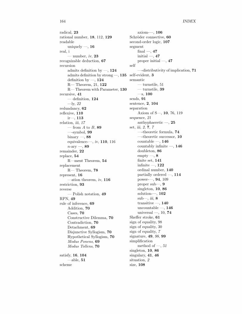
164 INDEX
radical, 23rational number, 18, 112, 129readable
uniquely —, 16real, i
— number, iv, 23recognizable deduction, 67recursion
admits definition by —, 124admits definition by strong—, 135definition by —, 124R— Theorem, 21, 122R—Theorem with Parameter, 130
recursive, 41— definition, 124—ly, 22
redundancy, 62reflexive, 110
ir—, 113relation, iii, 17
— from A to B, 89—-symbol, 99binary —, 88equivalence-—, iv, 110, 116n-ary —, 89
remainder, 22replace, 54
R—ment Theorem, 54replacement
R— Theorem, 78represent, 16
—ation theorem, iv, 116restriction, 93reverse
— Polish notation, 49RPN, 49rule of inference, 69
Addition, 70Cases, 70Constructive Dilemma, 70Contradiction, 70Detachment, 69Disjunctive Syllogism, 70Hypothetical Syllogism, 70Modus Ponens, 69Modus Tollens, 70
satisfy, 16, 104—able, 51
scheme
axiom-—, 106Schroder connective, 60second-order logic, 107segment
final —, 47initial —, 47proper initial —, 47
self—-distributivity of implication, 71
self-evident, 3semantic
— turnstile, 51— turnstile, 39—s, 100
sends, 91sentence, 2, 104separation
Axiom of S—, 10, 76, 119sequence, 21
anthyphaeretic —, 25set, iii, 2, 7, 7
—-theoretic formula, 74—-theoretic successor, 10countable —, 146countably infinite —, 146doubleton, 86empty —, 8finite set, 141infinite —, 122ordinal number, 140partially ordered —, 114power-—, 94, 109proper sub—, 9singleton, 10, 86solution-—, 102sub—, iii, 8transitive —, 140uncountable —, 146universal —, 10, 74
Sheffer stroke, 61sign of equality, 98sign of equality, 30sign of equality, 7signature, 49, 98, 99simplification
method of —, 51singleton, 10, 86singulary, 41, 46situation, 2size, 108
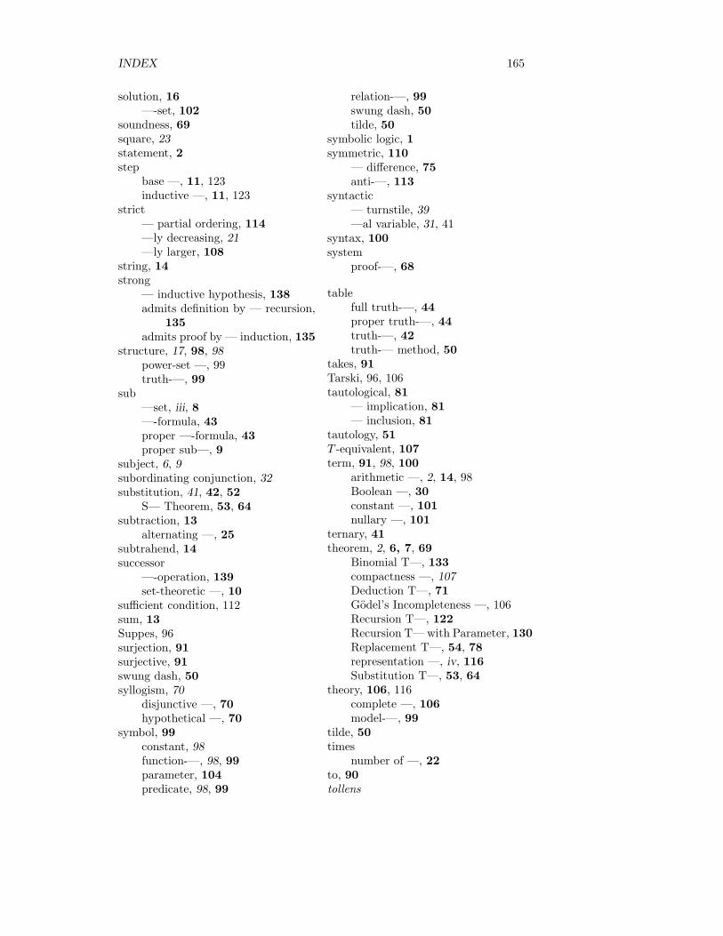
INDEX 165
solution, 16—-set, 102
soundness, 69square, 23statement, 2step
base —, 11, 123inductive —, 11, 123
strict— partial ordering, 114—ly decreasing, 21—ly larger, 108
string, 14strong
— inductive hypothesis, 138admits definition by — recursion,
135admits proof by — induction, 135
structure, 17, 98, 98power-set —, 99truth-—, 99
sub—set, iii, 8—-formula, 43proper —-formula, 43proper sub—, 9
subject, 6, 9subordinating conjunction, 32substitution, 41, 42, 52
S— Theorem, 53, 64subtraction, 13
alternating —, 25subtrahend, 14successor
—-operation, 139set-theoretic —, 10
sufficient condition, 112sum, 13Suppes, 96surjection, 91surjective, 91swung dash, 50syllogism, 70
disjunctive —, 70hypothetical —, 70
symbol, 99constant, 98function-—, 98, 99parameter, 104predicate, 98, 99
relation-—, 99swung dash, 50tilde, 50
symbolic logic, 1symmetric, 110
— difference, 75anti-—, 113
syntactic— turnstile, 39—al variable, 31, 41
syntax, 100system
proof-—, 68
tablefull truth-—, 44proper truth-—, 44truth-—, 42truth-— method, 50
takes, 91Tarski, 96, 106tautological, 81
— implication, 81— inclusion, 81
tautology, 51T -equivalent, 107term, 91, 98, 100
arithmetic —, 2, 14, 98Boolean —, 30constant —, 101nullary —, 101
ternary, 41theorem, 2, 6, 7, 69
Binomial T—, 133compactness —, 107Deduction T—, 71Godel’s Incompleteness —, 106Recursion T—, 122Recursion T—with Parameter, 130Replacement T—, 54, 78representation —, iv, 116Substitution T—, 53, 64
theory, 106, 116complete —, 106model-—, 99
tilde, 50times
number of —, 22to, 90tollens
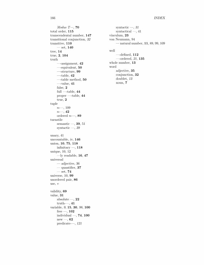
166 INDEX
Modus T—, 70total order, 115transcendental number, 147transitional conjunction, 32transitive, 110
— set, 140tree, 14true, 2, 104truth
—-assignment, 42—-equivalent, 50—-structure, 99—-table, 42—-table method, 50—-value, 41false, 2full —-table, 44proper —-table, 44true, 2
tuplen-—, 109n-—, 42ordered n-—, 89
turnstilesemantic —, 39, 51syntactic —, 39
unary, 41uncountable, iv, 146union, 10, 75, 118
infinitary —, 118unique, 10, 12
—ly readable, 16, 47universal
— adjective, 36— quantifier, 37— set, 74
universe, 10, 99unordered pair, 86use, v
validity, 69value, 31
absolute —, 22truth-—, 41
variable, 9, 15, 30, 98, 100free —, 102individual —, 74, 100new —, 62predicate-—, 121
syntactic —, 31syntactical —, 41
vinculum, 23von Neumann, 94
— natural number, 11, 89, 99, 109
well—-defined, 112—-ordered, 21, 135
whole number, 13word
adjective, 35conjunction, 32doublet, 13noun, 7


![CADASTRE SURVEY PRACTICE (SGHU 4323)...2018/11/13 · High-water mark of ordinary spring tides SEA BED [ X1,Y1, H1 ] [ X2,Y2, H1] [ X2,Y2, H2 ] [ X3,Y3, H1] [ X3,Y3, H2 ] [ X4,Y4,](https://static.fdocuments.us/doc/165x107/5fbc7b38fe1918776c7d22b0/cadastre-survey-practice-sghu-4323-20181113-high-water-mark-of-ordinary.jpg)