On the determinant of quaternionic polynomial matrices and its application to system stability

MATHEMATICAL METHODS IN THE APPLIED SCIENCESMath. Meth. Appl. Sci. 2008; 31:99–122Published online 25 May 2007 in Wiley InterScience(www.interscience.wiley.com) DOI: 10.1002/mma.901MOS subject classification: 93D 20; 15A 33; 15A 15; 15A 18

On the determinant of quaternionic polynomial matricesand its application to system stability

Ricardo Pereira∗,† and Paula Rocha

Department of Mathematics, University of Aveiro, Aveiro 3810-193, Portugal

Communicated by K. Guerlebeck

SUMMARY

In this paper, we propose a definition of determinant for quaternionic polynomial matrices inspired by thewell-known Dieudonne determinant for the constant case. This notion allows to characterize the stabilityof linear dynamical systems with quaternionic coefficients, yielding results which generalize the onesobtained for the real and complex cases. Copyright q 2007 John Wiley & Sons, Ltd.

KEY WORDS: quaternionic polynomial matrices; determinant; stability

1. INTRODUCTION

The research reported in this paper is motivated by the study of stability for linear dynamicalsystems with quaternionic coefficients. These systems can be used to model several physicalphenomena, for instance, in areas such as robotics and quantum mechanics. More concretely,quaternions are a powerful tool in the description of rotations [1]. There are situations, especially inrobotics, where the rotation of a rigid body depends on time, and this dynamics is advantageouslywritten in terms of quaternionic differential or difference equations. The effort to control therotation dynamics motivates the study of these equations from a system theoretic point of view(see, for instance, [2]). Another motivation stems from quantum mechanics, where a quaternionicformulation of the Schrodinger equation has been proposed in 1960s along with experimentsto check the existence of quaternionic potentials (see, for instance, [3]). This theory leads todifferential equations with quaternionic coefficients [4].

A common way to treat linear dynamical systems is to consider state space models. The stabilityof a linear state-space system x = Ax with real or complex coefficients is essentially characterized

∗Correspondence to: Ricardo Pereira, Department of Mathematics, University of Aveiro, Aveiro 3810-193, Portugal.†E-mail: [email protected]

Contract/grant sponsor: Portuguese Science Foundation

Copyright q 2007 John Wiley & Sons, Ltd. Received 18 July 2006

100 R. PEREIRA AND P. ROCHA

by the location of the eigenvalues of the system matrix A, involving thus the computation ofthe determinant of the polynomial matrix s I − A [5]. In a more general setting, the growth ofthe solutions (or trajectories) of a linear higher-order differential equation with constant (square)matrix coefficients (Rmdm/dtm + · · · + R1d/dt + R0)w = 0 can also be characterized in terms ofthe zeros of the determinant of the polynomial matrix R(s) := Rmsm + · · · + R1s + R0 [6].

When trying to generalize these results to the quaternionic case, we were confronted withthe lack of a notion of determinant for quaternionic polynomial matrices. Indeed, due to thenoncommutativity of the field of quaternions, the determinant of quaternionic matrices cannot bedefined as in the commutative (e.g. real or complex) case. Several definitions have been proposedfor matrices over the quaternionic skew field [7, 8], for instance, the Study determinant [9] (in1920) and latter, in the 1940s, the Dieudonne determinant [10]. Whereas the former is defined interms of complex adjoint matrices, the latter results from a direct approach that remains entirelyat the quaternionic level. However, up to our knowledge, this work has not been extended to thepolynomial ring case.

Considering complex adjoints for quaternionic polynomial matrices, as introduced in [11], theStudy determinant can be generalized in a straightforward manner. However, the natural questionarises whether it is possible to define a polynomial determinant without leaving the quaternionicframework, as happens with the Dieudonne determinant for the constant case. In this paper, wegive a positive answer to this question by introducing the polynomial determinant Pdet.

Further, we prove that, as should be expected, the zeros of Pdet(s I − A) are precisely the (right)eigenvalues of the quaternionic matrix A, which allows us to generalize the stability analysis oflinear dynamical systems to the quaternionic case.

2. PRELIMINARIES

2.1. Stability of linear systems

Systems described by linear differential equations with constant matrix coefficients(Rm

dm

dtm+ · · · + R1

d

dt+ R0

)w = 0 (1)

with R(s) := Rmsm + · · · + R1s + R0 ∈ Fn×n[s] and F the field R or C, can be considered as ageneralization of state-space systems:

x = Ax (2)

Such systems have been widely studied within the behavioural approach to dynamical systemsintroduced by Willems [12] with respect to various aspects. Here we are particularly interested inthe question of stability.

A linear system is said to be (asymptotically) stable if all its solutions tend to zero as timegoes to infinity. For systems described by an equation of type (2), stability is characterized by thefollowing proposition.

Proposition 2.1 (Kailath [5])The state system (2) is stable if and only if det(�I − A) �= 0, ∀� ∈ C+

0 , where C+0 := {z ∈ C :

Re(z)�0}.

Copyright q 2007 John Wiley & Sons, Ltd. Math. Meth. Appl. Sci. 2008; 31:99–122DOI: 10.1002/mma

DETERMINANT OF QUATERNIONIC POLYNOMIAL MATRICES 101

This result also generalizes to systems with description (1), as stated below.

Proposition 2.2 (Polderman and Willems [6])System (1) is stable if and only if det R(�) �= 0, ∀� ∈ C+

0 .

In this paper, we replace the field F by the quaternionic skew field H, to be properly definedin the next section. This gives rise to linear quaternionic systems, with trajectories evolvingover Hn .

In order to study the stability of such systems, we first introduce some preliminary concepts onquaternions and quaternionic polynomials and then, in Section 3, our notion of determinant forquaternionic polynomial matrices.

2.2. The quaternionic skew field

The set

H = {a + bi + cj + dk : a, b, c, d ∈ R}

where the imaginary units i, j, k satisfy i2 = j2 =k2 = ijk= −1 and, consequently,

ij= k= −ji, jk= i= −kj, ki= j= − ik

is an associative but noncommutative division algebra over R called quaternionic skew field.The real and imaginary parts of a quaternion � = a + bi + cj + dk are defined as Re � = a andIm � = bi + cj + dk, respectively, whereas, similar to the complex case, the conjugate � is givenby � = a − bi − cj − dk and the norm |�| is defined as |�| = √

��.Two quaternions � and � are said to be similar, � ∼ �, if there exists a nonzero � ∈ H such

that � = ��−1. Similarity is an equivalence relation and we denote by [�] the equivalence classcontaining �. Note that � ∈ [�], as a consequence of the following theorem.

Theorem 2.3 (Zhang [13])Given two quaternions �, � ∈ H, � ∈ [�] if and only if Re � =Re � and |�| = |�|.

This theorem also implies that every quaternion is similar to a complex number. Indeed, if� = a + bi + cj + dk∈ H then the complex z = a + √

b2 + c2 + d2i∈ C is similar to � sinceRe z =Re � and |z| = |�|.2.3. Quaternionic polynomials

In this section, we define the quaternionic polynomials to be considered in the sequel and studysome of their most relevant properties for our purposes. Unlike the real or complex case, there areseveral possible ways to define quaternionic polynomials since the coefficients can be taken to beon the right, on the left or on both sides of the indeterminate (see, e.g. [14]). In this paper, weshall adopt the following definition.

Definition 2.4A quaternionic polynomial p(s) is defined as

p(s) = pnsn + · · · + p1s + p0, pl ∈ H, l = 1, . . . , n



If pn �= 0, the degree of the quaternionic polynomial p(s), deg p(s), is n and its leading coefficient,lc p(s), is pn . As usual, if lc p(s) = 1, p(s) is said to be monic.

We denote by H[s] the set of quaternionic polynomials endowed with the following sum andproduct. Given two quaternionic polynomials p(s) = ∑N

n=0 pnsn and q(s)= ∑M

m=0 qmsm :

p(s) + q(s) =max{N ,M}∑

l=0(pl + ql)s

l

p(s)q(s) =N+M∑l=0

∑n+m=l

pnqmsl =: pq(s)

Clearly, H[s] is a noncommutative ring [15]. Note moreover that, with the defined operations, unlikethe commutative case, evaluation of polynomials is not a ring homomorphism, i.e. if r = pq ∈ H[s],then in general r(�) �= p(�)q(�), � ∈ H, as shown in the following example.

Example 2.5Let p(s) = s − i, q(s)= s − j and

r(s) = p(s)q(s)= (s − i)(s − j) = s2 − (i + j)s + k

Then

r(i) = i2 − (i + j)i − k= 2k but p(i)q(i)= (i − i)(i − j) = 0

To simplify the notation, we may omit the indeterminate and write p ∈ H[s], if no ambiguityarises.

A polynomial p(s) is said to be an invertible element or a unit of H[s] if there exists q(s)∈ H[s]such that q(s)p(s)= p(s)q(s)= 1. This clearly means that p(s) must be a nonzero quaternionicconstant.

Conjugacy is extended to quaternionic polynomials by linearity and by the rule asn = asn ,∀a ∈ H. As a consequence, pq = q p for every p, q ∈ H[s] (see [11]). Moreover, the followingresult holds.

Proposition 2.6 (Pereira et al. [11])Let p, q ∈ H[s]. Then

(i) pp= pp ∈ R[s].(ii) If pq ∈ R[s], then pq = qp.

Remark 2.7Note that in the particular case where p is monic and of degree 1, i.e. p(s) = s−�, � ∈ H, the productpp is an invariant of the similarity class of �. Indeed, pp= (s − �)(s − �) = s2 − 2(Re �)s + |�|2.Since, by Theorem 2.3, for all �′ ∼ � we have that Re � =Re �′ and |�| = |�′| it is clear that ifq(s)= s − �′, with � ∼ �′, then pp= qq.



A quaternionic polynomial d(s) is said to be a left divisor of a polynomial p(s) ∈ H[s], whichwe shall denote by d(s)|l p(s), or, equivalently, p(s) is said to be a right multiple of d(s), if thereexists a polynomial q(s) such that

p(s) = d(s)q(s)

If d(s) is a left divisor of both p(s) and q(s), and d(s) is a right multiple of every common leftdivisor of p(s) and q(s), then d(s) is a greatest common left divisor (gcld) of p(s) and q(s). Thegcld is unique up to right multiplication by a unit. Two polynomials p(s) and q(s) are called leftcoprime if every gcld of p(s) and q(s) is a unit.

The definitions of right divisor, gcrd, and right coprimeness (left multiple) are entirely analogous.We shall use the notation d(s)|r p(s) to indicate that d(s) is a right divisor of p(s).

In general, the gcld’s of two quaternionic polynomials are different from their gcrd’s.

Example 2.8Let p(s) = js − k and q(s)=−is + 1. Then every gcrd(p(s), q(s)) is of the form �(−is + 1),� ∈ H, and every gcld(p(s), q(s)) is a constant � ∈ H.

The zeros of a quaternionic polynomial p ∈ H[s] are the values � ∈ H such that p(�) = 0. Theproblem of finding such zeros as well as the study of the fundamental theorem of algebra for thequaternionic case were first addressed in the 1940s by Niven [16] and Niven and Eilenberg [17].This was followed by other contributions, such as [18, 19], where the questions of finding andcounting the number of zeros of quaternionic polynomials have been investigated.

A pair (p, q) ∈ H[s]2 is zero coprime if p and q do not have common zeros. Factors of apolynomial are usually related to its zeros, but the fact that evaluation is not a ring homomorphism,as mentioned before, implies that the relation between the factors and the zeros of a quaternionicpolynomial is not as simple as for real or complex polynomials. Results concerning this nontrivialrelation can be found in [20, 21].

The next proposition establishes a connection between zeros and right divisors.

Proposition 2.9 (Lam [21])A quaternion � is a zero of a nonzero p ∈ H[s] if and only if the polynomial s−� is a right divisorof p.

Note that this implies that zero coprimeness is equivalent to right coprimeness. However, ifd(s) is a left divisor of p(s), the zeros of d(s) are not necessarily zeros of p(s). For instance, inExample 2.5, p(s) = (s − i) is a left divisor of r(s), p(i) = 0 but r(i) = 2k �= 0.

Nevertheless, there is still some connection between the zeros of a polynomial and the zerosof its left divisors. Indeed, let r = pq ∈ H[s], if � ∈ H is a zero of the polynomial r but not of itsright divisor q , then its left divisor p must have a zero that is equivalent to �. This is formalizedin the following result.

Proposition 2.10 (Lam [21])Let r = pq ∈ H[s] and � ∈ H be such that � = q(�) �= 0. Then

r(�) = p(��−1)q(�)

In particular, � is a zero of r if and only if ��−1 is a zero of p.



Besides the similarity concept that we have been using up to this point, a second notion willplay an important role in the sequel. In order to distinguish it from the first one, we shall callit J -similarity, and denote it by ∼J , where the J stands for Jacobson, who first introduced thisnotion, [15].Definition 2.11 (Jacobson [15] and Cohn [22])Two quaternionic polynomials a, d ∈ H[s] are said to be J-similar, a ∼J d , if there exist b, c∈ H[s]such that the relation

ab= cd

is a coprime relation. By this, it is meant that (a, c) are left coprime and (b, d) are right coprime.

Our next result, that will be relevant in Section 3, relates the real polynomials aa and dd incase a ∼J d .

Proposition 2.12Let a = ∑n

l=0 alsl , d = ∑m

l=0 dlsl ∈ H[s] be such that |an| = |dm |.

If a ∼J d , i.e. there exist b, c∈ H[s] such that

ab= cd (3)

is a coprime relation, then

aa = dd and bb= cc

ProofSee Appendix A. �

2.4. Quaternionic polynomial matrices

As usual, Hg×r and Hg×r [s] will, respectively, denote the set of the g× r matrices with entriesin H and in H[s]. As for polynomials, for simplicity, we may also omit the indeterminate s andwrite R ∈ Hg×r [s] if no ambiguity arises.

A square matrix R ∈ Hg×g has full rank if for X ∈ H1×g , XR = 0 implies X = 0. The samedefinition holds for polynomial matrices.

A matrix U ∈ Hg×g[s] is said to be a unimodular polynomial matrix if there exists a polynomialmatrix V ∈ Hg×g[s] such that VU =UV = I , where I is the identity matrix.

According to [7] we shall use the following notation.

Notation 2.13Denote by Plm the matrix that is obtained from the identity by interchanging the lth and mth rows.Denote by Blm(�), where � ∈C and C is a set, the matrix that is obtained from the identity byadding the mth row multiplied by � to the lth row. Finally denote by SL(n,C) the set of all n × nmatrices that can be decomposed as a product of matrices of the types Plm and Blm(�), � ∈C.

As in the commutative case, it is possible to obtain a triangular matrix pre-multiplying theoriginal one by a matrix belonging to SL(n, H[s]). The result is formalized next. The proof is



completely analogous to the one of [6, Theorem B.1.1] and is based on the Euclidian divisionalgorithm.

Lemma 2.14For every R ∈ Hn×n[s] there exists a matrix U ∈ SL(n, H[s]) such that

UR = T

where T ∈ Hn×n[s] is a triangular matrix.

The following result is relevant for the definition of the determinant of quaternionic polynomialmatrices that will be given in Section 3.

Lemma 2.15Let

R =[

�1

�2

]∈ H2×1[s].

Then there exists U ∈ SL(n, H[s]) such that

UR =[u11 u12

u21 u22

][�1

�2

]=[t

0

]

with t a gcrd of �1 and �2, and letting g ∈ H[s] be such that �2 = gt ,

u21 ∼J g and |lcu21| = |lcg|

ProofSee Appendix A. �

3. POLYNOMIAL DETERMINANT

Before considering the polynomial case, it should be noticed that the question of defining adeterminant for constant quaternionic matrices is itself nontrivial and has deserved the attentionof several mathematicians throughout the years.

Indeed, due to the noncommutativity of the quaternionic skew field H, it is not possible toextend the usual definition of determinant. For instance, let

A=[i 0

0 j

]



and suppose that the usual properties for determinants of complex matrices would hold. Then

det A= det

[i 0

0 j

]= i det

[1 0

0 j

]= ij det

[1 0

0 1

]= ij= k

whereas, on the other hand

det A= det

[i 0

0 j

]= j det

[i 0

0 1

]= ji det

[1 0

0 1

]= ji=−k

leading to an absurd.The first mathematician who tried to define the determinant of a quaternionic matrix was

Cayley [23], but his definition was not satisfactory (see [7]). Only in the twentieth century newdevelopments in this topic were achieved. Moore [24] showed that the Cayley determinant makessense when restricted to hermitian quaternionic matrices and some different, but closely related,definitions such as the determinants of Study [9] and Dieudonne [10] were given. More recently,in the nineties, Gelfand and Retakh [25] introduced the notion of quasideterminant, but this isbeyond the scope of this article.

The determinants of Study and Dieudonne are in accordance with the following definition ofdeterminant for quaternionic matrices, that can be regarded as a generalization of the notion ofdeterminant for the real and complex cases.

Definition 3.1 (Aslaksen [7])A function d :Hn×n → H is said to be a determinant if it satisfies the following axioms:

(i) d(A)= 0 if and only if A has not full rank.(ii) d(AB)= d(A)d(B) for all A, B ∈ Hn×n .(iii) If A′ = Blm(�)A, � ∈ H, then d(A′) = d(A).

We shall also adopt this definition for the polynomial case and say that d :Hn×n[s] → H[s] isa polynomial determinant if it satisfies the conditions of Definition 3.1, with H replaced by H[s].

The concrete notion of polynomial determinant that we propose is motivated by the definitionof Dieudonne determinant given below. First we state an auxiliary lemma.

Lemma 3.2 (Dieudonne [10])Let A∈ Hn×n be invertible. Then there exists a matrix U ∈ SL(n, H) such that

U A= diag(1, . . . , 1, �), � ∈ H

Definition 3.3 (Dieudonne [10])Let A∈ Hn×n; the Dieudonne determinant of A, denoted by Ddet(A), is defined as follows.

• If A has not full rank, then Ddet(A) := 0.• Otherwise, let U ∈ SL(n, H) be such that

U A= diag(1, . . . , 1, �), � ∈ H

Then Ddet(A) := |�|.



Dieudonne [10] shows that Ddet (also called normalized Dieudonne determinant in [7]) isequivalent to his determinant originally defined in more abstract terms.

Remark 3.4Note that the Dieudonne determinant is not an extension of the determinant of real matrices, i.e.given a real matrix A∈ Rn×n then, in general, Ddet(A) �= det(A). For instance, consider the simplescalar case A= −1. Then det(A) =−1 but Ddet(A) = |−1| = 1.

The straightforward extension of the Dieudonne determinant to the polynomial case faces twomajor difficulties. First it is impossible to diagonalize a polynomial matrix R ∈ Hn×n[s] as inLemma 3.2, i.e. only multiplying on the left by a matrix U ∈ SL(n, H[s]). Second it does notmake sense to define the norm of a polynomial.

However, as seen in Lemma 2.14, given a matrix R ∈ Hn×n[s] there exists a matrix U ∈ SL(n,

H[s]) such that UR = T , where T is a triangular polynomial matrix. Using an approach in somesense similar to the one of Dieudonne, we define a polynomial determinant for the quaternionicpolynomial matrix R with basis on the diagonal elements of the triangular matrix T .

Definition 3.5We define the function Pdet(·) :Hn×n[s] → R[s] as follows.

Let R ∈ Hn×n[s]. Let further U ∈ SL(n, H[s]) be such that UR is upper triangular, i.e.

UR = T =

⎡⎢⎢⎢⎢⎢⎢⎢⎢⎢⎣

�1 ∗ · · · ∗ ∗0 �2

. . ....

...

0 0. . . ∗ ∗

......

. . . �n−1 ∗0 0 · · · 0 �n

⎤⎥⎥⎥⎥⎥⎥⎥⎥⎥⎦(4)

Then

Pdet(R) :=n∏

l=1�l�l

Note that Definition 3.5 is well posed as a consequence of the following lemma.

Lemma 3.6Given R ∈ Hn×n[s], let T and T ′ be two triangular matrices obtained by pre-multiplying R by Uand U ′ ∈ SL(n, H[s]), respectively. Let further �1, . . . , �n and �′

1, . . . , �′n be the elements of the

main diagonal of T and T ′, respectively. Thenn∏

l=1�′l�

′l =

n∏l=1

�l�l (5)

ProofIf R has not full rank, the same happens for every triangular matrix T such that UR = T , for someU ∈ SL(n, H[s]. This clearly implies that at least one of the diagonal elements of T is zero, andthe same happens with T ′. Therefore (5) holds since both sides of the equality are zero.



Let now R have full rank. Suppose first that R ∈ H2×2[s] is triangular and 2× 2, i.e.

R =[

�1 �12

0 �2

]with �1, �2 �= 0

Let

U =[u11 u12

u21 u22

]∈ SL(2, H[s])

be such that

UR =[u11 u12

u21 u22

][�1 �12

0 �2

]=[u11�1 u11�12 + u12�2

u21�1 u21�12 + u22�2

]=[

�′1 �′

12

0 �′2

]= T ′

Then u21�1 = 0, i.e. u21 = 0 and thereforeU is triangular. Taking into account thatU ∈ SL(2, H[s]),this implies that u11 and u22 are nonzero constants, i.e. u11, u22 ∈ H\{0}. We next show that|u11||u22| = 1. Indeed, it is not difficult to see that there exists V ∈ SL(2, H[s]) such that

VU =[1 0

0 u11u22

]

Since VU ∈ SL(2, H[s]) and it is a constant matrix, this implies that VU ∈ SL(2, H). Conse-quently, the Dieudonne determinant of VU must be equal to 1, i.e.

Ddet(VU ) = |u11u22| = |u11||u22| = 1

Recall that, as mentioned in Section 2.3, for every p, q ∈ H[s], pp ∈ R[s] and p q = qp. Hence,

�′1�

′1�

′2�

′2 = u11�1�1u11u22�2�2u22 = �1�1�2�2|u11|2|u22|2 = �1�1�2�2

If R ∈ Hn×n[s] is triangular and U ∈ SL(n, H[s]) is such that UR = T ′, with T ′ triangular, analo-gously to the previous case the matrix U must also be triangular and the product of the norms ofits main diagonal elements is equal to 1. Thus, equality (5) holds.

Finally, consider the case where R is not triangular. Let U,U ′ ∈ SL(n, H[s]) be such that

UR = T, U ′R = T ′ with T, T ′ triangular

Then

T ′ =U ′R =U ′U−1UR =U ′′T

where U ′′ =U ′U−1 ∈ SL(n, H[s]), and, by the previous case, we can conclude that equality (5)holds.



Example 3.7Let

R(s)=[

(s + 2j)(s + j) (s + 2j)(2s + k)(s + 3i) + 2s + 3

s + j (2s + k)(s + 3i)

]

Then

R =UT =[s + 2j 1

1 0

][s + j (2s + k)(s + 3i)

0 2s + 3

]

and U ∈ SL(n, H[s]). ThereforePdet(R) = (s + j)(s + j)(2s + 3)(2s + 3) = (s2 + 1)(2s + 3)2

We next show that Pdet(·) is indeed a polynomial determinant. For that purpose we first provean auxiliary result that states that it is invariant with respect to post-multiplications by a matrixU ∈ SL(n, H[s]).Lemma 3.8Let M ∈ Hn×n[s] and U ∈ SL(n, H[s]). Then

Pdet(MU )=Pdet(M) (6)

ProofSince U ∈ SL(n, H[s]) is a finite product of Plm and Blm(�) matrices, � ∈ H[s], it is clearly enoughto prove that

Pdet(MS)=Pdet(M)

if S is Plm or Blm(�) matrix, � ∈ H[s].If M has not full rank, equality (6) trivially holds.If M has full rank, there exists a matrix V ∈ SL(n, H[s]) such that T = V M , where T is a

triangular matrix, and consequently Pdet(M)=Pdet(T ). Thus

Pdet(MS)=Pdet(V MS)=Pdet(T S)

and it is therefore sufficient to show that Pdet(T S)= Pdet(S).Suppose first that T ∈ H2×2[s] and is given by

T =[

�1 �12

0 �2

]with �1, �2 �= 0 and hence Pdet(T ) = �1�1�2�2 (7)

In the sequel, we show that Pdet(T S)=Pdet(T ), where S = B12(�), � ∈ H[s], or S = P12. Note thatit is not necessary to prove that Pdet(T S) =Pdet(T ) with S = B21(�) since B21(�) = P12B12(�)P12.



The first case is obvious because

T B12(�) =[

�1 �12

0 �2

][1 �

0 1

]=[

�1 �1� + �12

0 �2

]

On the other hand,

T P12 =[

�1 �12

0 �2

][0 1

1 0

]=[

�12 �1

�2 0

]= T ′

By Lemma 2.15, there exists a matrix V =[

v11v21

v12v22

]∈ SL(n, H[s]) such that

VT ′ =[

v11 v12

v21 v22

][�12 �1

�2 0

]=[

�′1 v11�1

0 v21�1

]

where �′1 is a gcrd of �12 and �2, and letting g be such that �2 = g�′

1, v21 ∼J g and |lc v21| = |lc g|.Therefore

Pdet(T P12) =Pdet(T ′) = �′1�

′1v21�1v21�1 = �′

1�′1v21v21�1�1

By Proposition 2.12, v21v21 = gg, and thus, since �2�2 = g�′1g�

′1 = �′

1�′1gg, by (7)

Pdet(T P12) = �′1�

′1v21v21�1�1 = �′

1�′1gg�1�1 = �2�2�1�1 =Pdet(T )

The case where T ∈ Hn×n[s] can be treated with basis on the previous one. In fact, if S = Blm(�),� ∈ H[s], the proof that Pdet(T S)= Pdet(T ) is analogous to the 2× 2 case. Moreover, note thatPlm can be written as a product of matrices Pr(r+1), i.e. matrices that are obtained from the identityby changing consecutive rows. Indeed,

Plm =(m−1∏r=l

Pr(r+1)

)(−l∏

r=2−mP(−r)(−r+1)

)

for instance

P14 = P12P23P34P23P12

The proof that Pdet(T Pr(r+1)) =Pdet(T ) is analogous to the 2× 2 case and the result follows.�

Proposition 3.9Pdet is a polynomial determinant, i.e.

(i) Pdet(R) = 0 if and only if R has not full rank.(ii) Pdet(RR′) =Pdet(R)Pdet(R′) for all R, R′ ∈ Hn×n[s].(iii) If R′ = Blm(�)R, � ∈ H[s], then Pdet(R′) = Pdet(R).



Proof(i) If R has not full rank and UR = T , for some U ∈ SL(n, H[s] and T a triangular matrix, thenT has not full rank. Therefore one of it its main diagonal elements is zero and hence Pdet(T ) = 0.On the other hand, let UR = T , with U and T as in Definition 3.5. If Pdet(R) = 0, then thereexists l = 1, . . . , n such that �l = 0. It is easy to check that this implies that the matrix T has notfull rank, which implies that R has not full rank.

(ii) Let R, R′ ∈ Hn×n[s] and U,U ′ ∈ SL(n, H[s]) be such that

UR = T, U ′R′ = T ′ (8)

where T and T ′ are triangular matrices whose main diagonal elements are, respectively, �l and �′l ,

l = 1, . . . , n.By definition, we have

Pdet(R) =n∏

l=1�l�l and Pdet(R′) =

n∏l=1

�′l�

′l

Therefore

Pdet(R)Pdet(R′) =n∏

l=1�l�l�

′l�

′l =

n∏l=1

�l�′l�

′l�l =

n∏l=1

�l�′l�l�

′l (9)

Now, note that by (8)

URR′ = T R′ = TU ′−1T ′ (10)

Let V ∈ SL(n, H[s]) be such that TU ′−1 = V T , with T triangular. It follows from Lemma 3.8 that

Pdet(T ) =Pdet(TU ′−1) =Pdet(T ) (11)

moreover by (10)

V−1URR′ = T T ′

Thus, since V−1U ∈ SL(n, H[s]),

Pdet(RR′) =Pdet(T T ′) = Pdet(T )Pdet(T ′)

taking into account that the main diagonal elements of T T ′ are the product of the main diagonalelements of T and T ′. Finally, since from (11) Pdet(T ) =Pdet(T ), we conclude that

Pdet(RR′) =Pdet(T )Pdet(T ′) = Pdet(T )Pdet(T ′) =Pdet(R)Pdet(R′)

(iii) By (ii), Pdet(R′) =Pdet(Blm(�)R) =Pdet(Blm(�))Pdet(R). The result follows since it isobvious that Pdet(Blm(�))= 1. �



Recalling Definition 3.3 of the Dieudonne determinant Ddet, note that if R is a constant matrix,i.e. R ∈ Hn×n ,

Pdet(R) = [Ddet(R)]2

Indeed, by Lemma 3.2, there exists a matrix U ∈ SL(n, H) such that UR = diag(1, . . . , 1, �), with� ∈ H. Hence Ddet(R) = |�| and Pdet(R) = �� = |�|2.

On the other hand, in [9] the Study determinant Sdet of a matrix R ∈ Hn×n is introduced as thedeterminant of its complex adjoint matrix

Rc =[

R1 R2

−R2 R1

]

where R1 and R2 are complex adjoint matrices such that R = R1 + R2j. Since, as shown in [7],Sdet(R) =[Ddet(R)]2 we conclude that

Sdet(R)= Pdet(R) (12)

Now, in the polynomial case, defining the complex adjoint Rc(s) of a matrix R(s) ∈ Hn×n[s] andits Study determinant Sdet(R(s)) in the obvious way, it can be shown [26, Theorem 3.3.5] that

Sdet(R(s))=Pdet(R(s))

which generalizes relation (12) for the polynomial case.

4. EIGENVALUES

In this section we show that, as should be expected, the zeros of Pdet(s I − A) coincide with theright eigenvalues of A.

A quaternion � is said to be a right eigenvalue of A∈ Hn×n if Av = v�, for some nonzeroquaternionic vector v ∈ Hn . The vector v is called a right eigenvector associated with �. The set

�r (A) ={� ∈ H : Av = v�, for some v �= 0}

is called the right spectrum of A. An efficient algorithm to calculate the right eigenvalues ofquaternionic matrices can be found in [27].

The following proposition plays an important role in the proof of Theorem 4.2.

Proposition 4.1 (Brenner [28])Let A∈ Hn×n . Then

� ∈ �r (A) ⇒ [�] ⊆ �r (A)

where [�] denotes the equivalence class of � (cf. p. 3).



Theorem 4.2‡Let A ∈ Hn×n . Then

� ∈ �r (A) ⇔ � is a zero of Pdet(s I − A)

ProofAssume first that A is full rank (invertible). Then, as happens for real matrices, there exists aninvertible matrix S ∈ Hn×n such that A′ = S−1AS is a companion matrix, i.e. has the form

A′ :=

⎡⎢⎢⎢⎢⎢⎢⎢⎢⎣

0 1 0 · · · 0

0 0 1 · · · 0

......

.... . .

...

0 0 0 · · · 1

−a0 −a1 −a2 · · · −an−1

⎤⎥⎥⎥⎥⎥⎥⎥⎥⎦∈ Hn×n

Note that �r (A′) = �r (A). Indeed, A′v = v� for some nonzero v ∈ Hn if and only if A′v′ = v′�,where v′ = Sv. On the other hand, s I − A= s I − SA′S−1 = S(s I − A′)S−1, which implies thatPdet(s I − A) =Pdet(s I − A′). Moreover, it is not difficult to see that there exist matrices P andQ ∈ SL(n, H[s]) such that

P(s I − A′)Q = diag(−1, . . . , −1, d(s))=: D

with d(s)= sn + an−1sn−1 + · · · + a1s + a0 ∈ H[s]. Then,

Pdet(s I − A′) =Pdet(P−1DQ−1) =Pdet(P−1)Pdet(D)Pdet(Q−1) = dd

Hence it suffices to prove that

� ∈ �r (A′) ⇔ � is a zero of dd

‡In [22], Theorem 8.5.1 states that if d(s) ∈ H[s] and A is the companion matrix of d(s) then � ∈ �r (A) if and onlyif d(�) = 0. However that result is not true. Indeed, if d(s) = s2 − (i + j)s + k, the companion matrix of d(s) is

A=[

0 1

−k i + j

]

it turns out that i is a right eigenvalue of A associated with the eigenvector

v =[

i + j

−1 − k

]

but d(i) = 2k �= 0. Nevertheless, i is a zero of Pdet(s I − A) = (s2 + 1)2.



‘⇐’ Let � be a zero of dd. By Proposition 2.6, � is a zero of dd , i.e. (dd)(�) = 0. If d(�) = 0,i.e. �n + an−1�

n−1 + · · · + a1� + a0 = 0, it is immediate that A′v = v�, with v = [1 � · · · �n−1]T.Hence � ∈ �r (A′).

On the other hand, suppose that d(�) �= 0. Since, by hypothesis (dd)(�) = 0, by Proposition 2.10there exists �′ ∈ [�] such that d(�′) = 0. This implies, by [21, Theorem 16.4], that there exists�′′ ∈ [�′] = [�] such that d(�′′) = 0. From the previous case, we conclude that �′′ ∈ �r (A′) which,by Proposition 4.1, implies that � ∈ �r (A′).

‘⇒’ Let � ∈ �r (A′), i.e. A′v = v�, for some nonzero v =[v1 · · · vn]T ∈ Hn . Then⎧⎪⎪⎪⎪⎨⎪⎪⎪⎪⎩v2 = v1�

· · ·vn = vn−1�

−a0v1 − a1v2 − · · · − an−1vn = vn�

(13)

If v1 = 0 it follows from (13) that v2 = · · · = vn = 0 and thus we assume that v1 �= 0. Suppose firstthat v1 = 1. In this case, from (13) we have that

�n + an−1�n−1 + · · · + a1� + a0 = 0

i.e. d(�) = 0. By Proposition 2.9 this implies that (dd)(�) = 0. Suppose now that v1 �= 1 and definev := vv−1

1 ∈Hn and � := v1�v−11 ∈ H. Note that v1 = 1 and � ∈ [�]. Then

A′v = v� ⇔ A′vv−11 = vv−1

1 v1�v−11 ⇔ A′v = v�

and therefore � ∈ �r (A′). Analogously to the previous case we conclude that d (�) = 0. By [11,Lemma 4.2], this implies that (dd)(�) = 0 for all � ∈ [�] and hence (dd)(�) = 0.

Suppose now that A is not invertible. Let V ∈ Hn×n be a change of coordinates that reduces A toits Jordan form J = V AV−1, [13]. By the same arguments as before, it is clear that �r (J )= �r (A)

and Pdet(s I − J ) =Pdet(s I −A). Therefore, we shall assume without loss of generality that A= J .Since A is not invertible it will have the block diagonal form A := diag(N , A), where

N :=

⎡⎢⎢⎢⎢⎢⎢⎢⎣

0 ∗ · · · ∗

0 0. . .

...

......

. . . ∗0 0 · · · 0

⎤⎥⎥⎥⎥⎥⎥⎥⎦∈ Hr×r and A∈ H(n−r)×(n−r) is invertible

Note that Pdet(s I − A) = s2rPdet(s I − A). Hence, denoting by N(M(s)) the set of zeros ofPdetM , N(s I − A) ={0} ∪ N(s I − A). On the other hand, �r (A) = {0} ∪ �r ( A). Thus, since Ais invertible, it follows from the first part that N(s I− A)=�r ( A), yielding the desired result. �



Corollary 4.3Let R(s) = Insm + Rm−1sm−1 + · · · + R1s + R0 ∈ Hn×n[s] and

A=

⎡⎢⎢⎢⎢⎢⎢⎢⎢⎣

0 In 0 · · · 0

0 0 In · · · 0

......

.... . .

...

0 0 0 · · · In

−R0 −R1 −R2 · · · −Rm−1

⎤⎥⎥⎥⎥⎥⎥⎥⎥⎦∈ Hmn×mn

be the block companion matrix of R. Then

� ∈ �r (A) ⇔ (Pdet R)(�) = 0

ProofConsider the matrix (s I − A) ∈ Hmn×mn[s]. It is not difficult to check that, as happens for realmatrices, there exist two matrices P and Q ∈ SL(mn, H[s]) such that P(s I − A)Q = D, where Dis block diagonal matrix

D := diag(−I, . . . , −I, R(s))

Then, it is clear that

Pdet(s I − A) =Pdet(P−1DQ−1) =Pdet(P−1)Pdet(D)Pdet(Q−1) =Pdet(R)

Thus, the result follows from Theorem 4.2. �

5. STABILITY CRITERION

With the definition of the polynomial determinant Pdet for quaternionic polynomial matrices givenin the previous section, we are now in a position to extend the results on system stability presentedin Section 2.1 to the quaternionic case.

Let us first consider a quaternionic state-space system

x = Ax (14)

with A∈ Hn×n . The solutions of (14) are given by [29]x(t) = eAt x0, x0 ∈ Hn (15)

where the exponential is defined as usual. If S ∈ Hn×n is a change of coordinates that reduces Ato its Jordan form J = SAS−1, (15) can still be written as

x(t) = eJ t x0, x0 ∈ Hn

x = S−1 x(16)



Taking into account the special structure of the Jordan form, it is possible to prove that thecomponents of x(t) are given by

e�t p(t)

where the �’s are the elements in the diagonal of J and p(t) is a suitable quaternionic polynomial.On the other hand, if � is a diagonal element of J , there exists a suitable initial value x0 = Er

(where Er is the r th vector of the canonical basis of Rn ⊂ Hn) such that

x(t) = e�t Er

It turns out that the elements in the diagonal of J correspond to the standard§ right eigenvaluesof A. Together with Theorem 4.2, this allows to characterize the stability of x = Ax in terms ofthe right spectrum �r (A) of A, or equivalently, in terms of the zeros of Pdet(s I − A).

Proposition 5.1Let A∈ Hn×n . Then the following statements are equivalent:

(i) The quaternionic system described by x = Ax is stable.(ii) �r (A) ⊂ H− := {q ∈ H : Re q<0}.(iii) All the zeros of Pdet(s I − A) lie in H−.

ProofThe equivalence between (ii) and (iii) is a direct consequence of Theorem 4.2.

(i) ⇒ (ii) If �r (A) /⊂ H−, there exists a standard right eigenvalue � of A such that Re ��0. Thus,keeping the notation of the previous considerations, for a suitable r , x(t)= S−1e�t Er , is a solutionof x = Ax . Since, obviously, limt→+∞ x(t) �= 0 the system is not stable.

(ii) ⇒ (i) If �r (A) ⊂ H−, then limt→+∞ x(t) = limt→+∞ eJ t x0 = 0, for all x0 ∈ Hn . By (16),this clearly implies that limt→+∞ x(t) = 0, for every solution x(t) of x = Ax , proving that thesystem is stable. �

Consider now a quaternionic system described by a higher-order matrix differential equation

R

(d

dt

)w = 0 (17)

with R(s) := Rmsm + · · · + R1s + R0 ∈ Hn×n[s]. Assume first that R(s) has full rank. Followingthe same kind of arguments as in [12], it is possible to show that there exists a unimodular matrixU (s)∈ Hn×n[s] such that

U (s)R(s)= Insm + Rm−1s

m−1 + · · · + R1s + R0 =: R(s)

§The standard right eigenvalues of a matrix A∈ Hn×n are the complex right eigenvalues of A with nonnegativeimaginary part.



Defining x := [wT wT · · · (w(m−1))T]T, we obtain the alternative system description{x = Ax

w =Cx(18)

with

A=

⎡⎢⎢⎢⎢⎢⎢⎢⎢⎣

0 In 0 · · · 0

0 0 In · · · 0

......

.... . .

...

0 0 0 · · · In

−R0 −R1 −R2 · · · −Rm−1

⎤⎥⎥⎥⎥⎥⎥⎥⎥⎦and C =[In 0 · · · 0]

Note that the pair (C, A) is observable, i.e.

rank

⎡⎢⎢⎢⎢⎢⎢⎣C

CA

...

CAl−1

⎤⎥⎥⎥⎥⎥⎥⎦ = l with l = nm

This is equivalent to say that [s I − A

C

]

has a left inverse [6] V (s). Therefore, it follows from (18) that

x(t) = V

(d

dt

)[0I

]w(t)

Together with the second equation of (18) this implies that limt→+∞ w(t)= 0 if and only iflimt→+∞ x(t) = 0. Hence the stability of the original system is equivalent to the stability of (18),which in turn, by Corollary 4.3 is equivalent to say that all the zeros of Pdet R(s) lie in H−.

If R(s) has not full rank, Pdet R(s)≡ 0. In this case, the corresponding system is not stable,since (as happens for real systems [12]) w will have some components that can be freely assigned,and hence can be chosen not to tend to zero.

We conclude in this way that stability of (17) can be characterized in terms of the zeros ofPdet R(s) as follows.



Theorem 5.2Consider the system

R

(d

dt

)w = 0 (19)

with R(s) := Rmsm + · · · + R1s + R0 ∈ Hn×n[s]. This system is stable if and only if

(Pdet R)(�) �= 0 ∀� ∈ H such that Re(�)�0

6. CONCLUSIONS

In this paper, a definition of determinant for quaternionic polynomial matrices was proposed,which has been inspired by the Dieudonne approach to the nonpolynomial case. Using this newconcept, a relationship was established between the right eigenvalues of a quaternionic matrix Aand the zeros of Pdet(s I − A) providing a correct formulation for a result suggested by Cohn [22].This enabled a characterization of the stability of linear systems with quaternionic coefficients,R(d/dt)w = 0, in terms of the zeros of Pdet(R(s)), that generalizes the results obtained for thereal and complex cases.

APPENDIX A

A.1. Proof of Proposition 2.12

Suppose first that a and d are monic.Let �1 ∈ H be such that d(�1) = 0. By Proposition 2.9, d(s)= d(s)(s − �1), i.e. c(s)d(s)=

c(s)d(s)(s−�1), which implies that (cd)(�1) = 0. Then, by (3), (ab)(�1) = 0 but b(�1) �= 0 because(b, d) are right coprime. Thus, by Proposition 2.10 there exists �′

1 = b(�1)�1b(�1)−1 ∼ �1 such thata(�′

1) = 0, i.e. a(s)= a(s)(s−�′1) for some a ∈ H[s]. This implies that a(s)b(s)= a(s)(s−�′

1)b(s).Moreover, by Proposition 2.10

((s − �′1)b(s))(�1) = (�′

1 − �′1)b(�1) = 0

and hence (s − �′1)b(s)= b(s)(s − �1), for some b∈ H[s]. Thusa(s)b(s)= c(s)d(s) ⇔ a(s )b(s)(s − �1) = c(s)d(s)(s − �1)

⇔ a(s )b(s) = c(s)d(s)

Note that both a(s) and d(s) are monic. Proceeding analogously as many times as necessary it ispossible to cancel out all the factors of d(s), i.e if

d(s)= (s − �m) · · · (s − �1), �l ∈ H, l = 1, . . . ,m (A1)

we obtain a(s )b(s) = c(s) with{a(s)= a(s)(s − �′m) · · · (s − �′

1), �′l ∼ �l , l = 1, . . . ,m

(s − �′m) · · · (s − �′

1)b(s)= b(s)(s − �m) · · · (s − �1)(A2)



Since a(s) is monic so is a(s). If we prove that a(s)= 1, by (A1) and the first equation of (A2)and as a consequence of Remark 2.7, we have that aa = dd as desired.

Since (a, c) are left coprime by hypothesis, it is clear that also (a, c) are left coprime, whichimplies that their conjugates (a, c) are right coprime. Moreover,

a(s )b(s) = c(s) ⇔ b(s )a(s)= c(s)

In the same way as the factors of d(s) were cancelled out, it is possible to cancel out all the factorsof c and, letting c(s) = (s − �r ) · · · (s − �1), �l ∈ H, l = 1, . . . , r , we get b′(s)a′(s)= 1, with{

b(s) = b′(s)(s − �′r ) · · · (s − �′

1), �′l ∼ �l , l = 1, . . . , r

(s − �′r ) · · · (s − �′

1)a(s) = a′(s)(s − �r ) · · · (s − �1)(A3)

By the second equation of (A3), since a(s) is monic so is a′(s). Moreover, b′(s)a′(s)= 1 impliesthat a′(s) = 1 and hence also a = 1, i.e. a = 1 and thus, as we stated above,

aa = dd (A4)

Furthermore, ab= cd ⇔ ba = dc which, by (A4), implies that

abba = cddc ⇔ aabb= ddcc ⇔ aa(bb − cc) = 0 ⇔ bb= cc

If a and d are not monic, define the quaternions

� := an|an|2 and � := dm

|dm |2

Then, due to the assumption that |an| = |dm |,

��= anan|an|4 = 1

|an|2 = 1

|dm |2 = ��

Define also the polynomials

a(s)= a(s)�, c(s) = c(s)�−1, b(s)= �−1b(s), d(s) = �d(s)

Since by hypothesis (a, c) are left coprime and (b, d) are right coprime, also (a, c) are left coprimeand (b, d) are right coprime. Now

a(s)b(s)= c(s)d(s) ⇔ a(s)��−1b(s)= c(s)�−1�d(s) ⇔ a(s )b(s) = c(s)d(s)

where a(s) and d(s) are monic and a ∼J d , and the result follows then from the first part of theproof. �



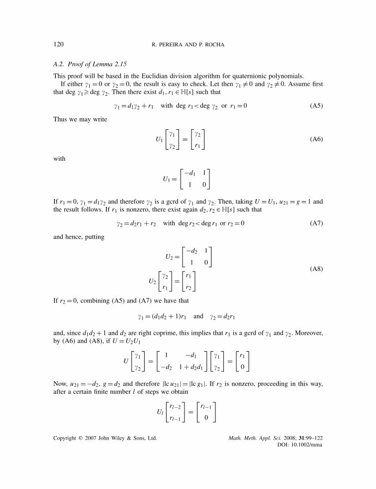
A.2. Proof of Lemma 2.15

This proof will be based in the Euclidian division algorithm for quaternionic polynomials.If either �1 = 0 or �2 = 0, the result is easy to check. Let then �1 �= 0 and �2 �= 0. Assume first

that deg �1� deg �2. Then there exist d1, r1 ∈ H[s] such that

�1 = d1�2 + r1 with deg r1< deg �2 or r1 = 0 (A5)

Thus we may write

U1

[�1

�2

]=[

�2

r1

](A6)

with

U1 =[−d1 1

1 0

]

If r1 = 0, �1 = d1�2 and therefore �2 is a gcrd of �1 and �2. Then, taking U =U1, u21 = g= 1 andthe result follows. If r1 is nonzero, there exist again d2, r2 ∈ H[s] such that

�2 = d2r1 + r2 with deg r2< deg r1 or r2 = 0 (A7)

and hence, putting

U2 =[−d2 1

1 0

]

U2

[�2

r1

]=[r1

r2

] (A8)

If r2 = 0, combining (A5) and (A7) we have that

�1 = (d1d2 + 1)r1 and �2 = d2r1

and, since d1d2 + 1 and d2 are right coprime, this implies that r1 is a gcrd of �1 and �2. Moreover,by (A6) and (A8), if U =U2U1

U

[�1

�2

]=[

1 −d1

−d2 1 + d2d1

][�1

�2

]=[r1

0

]

Now, u21 =−d2, g= d2 and therefore |lc u21| = |lc g1|. If r2 is nonzero, proceeding in this way,after a certain finite number l of steps we obtain

Ul

[rl−2

rl−1

]=[rl−1

0

]



and

�1 = grl−1

�2 = grl−1, r0 = �2(A9)

with g= d1d2 · · · dl + lower-order terms (l.o.t) and g= d2d3 · · · dl + l.o.t.Thus

U

[�1

�2

]=[t

0

](A10)

with U =Ul · · ·U1 and t = rl−1. Further, it is not difficult to see that

u21 = (−1)l−1dl · · · d2 + l.o.t

u22 = (−1)ldl · · · d2d1 + l.o.t(A11)

Note that, by (A9) and (A10), we can conclude that t is a gcrd of �1 and �2. Moreover |lc u21| = |lc g|since |lc u21| = |lc dl | · · · |lc d2| = |lc d2| · · · |lc dl | = |lc g|. Now, it still remains to prove that u21 ∼Jg. Clearly g and g are right coprime and since the matrix U is unimodular its elements u21 and u22are left coprime. Moreover, from Equation (A10) we obtain u21�1 +u22�2 = 0, which is equivalentto u21g2 + u22g1 = 0. Thus, by Definition 2.11 it follows that u21 ∼J g.

The case where deg �2� deg �1 is analogous to the previous one. Indeed, with the followingmultiplication [

0 1

1 0

][�1

�2

]=[

�2

�1

]

we fall into the previous case, where the expressions for �1 and �2 in (A9) as well as the expressionsfor u21 and u22 in (A11) are interchanged. It is clear that the result still holds. �

ACKNOWLEDGEMENTS

This work was supported in part by Portuguese Science Foundation (FCT—Fundacao para a Cienciae Tecnologia) through the Unidade de Investigacao Matematica e Aplicacoes of University of Aveiro,Portugal.

REFERENCES

1. Kuipers JB. Quaternions and Rotation Sequences. Princeton University Press: Princeton, NJ, 1999.2. El-Gohary A, Elazab ER. Exponential control of a rotational motion of a rigid body using quaternions. Applied

Mathematics and Computation 2003; 137(2–3):195–207.3. De Leo S, Ducati GC, Nishi CC. Quaternionic potentials in non-relativistic quantum mechanics. Journal of

Physics A: Mathematical and General 2002; 35(26):5411–5426.4. De Leo S, Ducati GC. Real linear quaternionic differential operators. Computers and Mathematics with Applications

2004; 48(12):1893–1903.5. Kailath T. Linear Systems. Prentice-Hall: Englewood Cliffs, NJ, 1980.6. Polderman JW, Willems JC. Introduction to Mathematical Systems Theory: A Behavioral Approach. Texts in

Applied Mathematics, vol. 26. Springer: Berlin, 1997.



7. Aslaksen H. Quaternionic determinants. Mathematical Intelligencer 1996; 18(3):57–65.8. Cohen N, De Leo S. The quaternionic determinant. Electronic Journal of Linear Algebra 2000; 7:100–111.9. Study E. Zur Theorie der linearen Gleichungen. Acta Mathematica 1920; 42:1–61.

10. Dieudonne J. Les determinants sur un corps non commutatif. Bulletin de la Societe Mathematique de France1943; 71:27–45.

11. Pereira R, Rocha P, Vettori P. Algebraic tools for the study of quaternionic behavioral systems. Linear Algebraand its Applications 2005; 400:121–140.

12. Willems JC. Paradigms and puzzles in the theory of dynamical systems. IEEE Transactions on Automatic Control1991; 36(3):259–294.

13. Zhang ZY. An algebraic principle for the stability of difference operators. Journal of Differential Equations 1997;136(2):236–247.

14. Pumplun S, Walcher S. On the zeros of polynomials over quaternions. Communications in Algebra 2002;30(8):4007–4018.

15. Jacobson N. The Theory of Rings. American Mathematical Society: New York, 1943.16. Niven I. The roots of a quaternion. American Mathematical Monthly 1942; 49:386–388.17. Eilenberg S, Niven I. The ‘fundamental theorem of algebra’ for quaternions. Bulletin of the American Mathematical

Society 1944; 50:246–248.18. Gordon B, Motzkin TS. On the zeros of polynomials over division rings. Transactions of the American

Mathematical Society 1965; 116:218–226.19. Serodio R, Pereira E, Vitoria J. Computing the zeros of quaternion polynomials. Computers and Mathematics

with Applications 2001; 42(8–9):1229–1237.20. Lee HC. Eigenvalues and canonical forms of matrices with quaternion coefficients. Proceedings of the Royal

Irish Academy Section A 1949; 52:253–260.21. Lam TY. A First Course in Noncommutative Rings. Springer: New York, 1991.22. Cohn PM. Skew Fields. Encyclopedia of Mathematics and its Applications, vol. 57. Cambridge University Press:

Cambridge, 1995.23. Cayley A. On certain results relating to quaternions. Philosophical Magazine 1845; 26:141–145.24. Moore EH. On the determinant of an Hermitian matrix of quaternionic elements. American MS Bulletin 1922;

28:161–162.25. Gelfand I, Retakh V. Quasideterminants. I. Selecta Mathematica, New Series 1997; 3(4):517–546.26. Pereira R. Quaternionic polynomials and behavioral systems. Ph.D. Thesis, University of Aveiro, 2006,

http://193.136.81.248/dspace/bitstream/2052/134/1/TesePhDRicardoPereira.pdf27. Bunse-Gerstner A, Byers R, Mehrmann V. A quaternion QR-algorithm. Numerische Mathematik 1989; 55(1):

83–95.28. Brenner JL. Matrices of quaternions. Pacific Journal of Mathematics 1951; 1:329–335.29. Hazewinkel M, Lewis J, Martin C. Symmetric systems with semisimple structure algebra: the quaternionic case.

Systems and Control Letters 1983; 3(3):151–154.


On the determinant of quaternionic polynomial matrices and its application to system stability

Documents

Transcript of On the determinant of quaternionic polynomial matrices and its application to system stability