Topics

Emin Gahramanov*

On the Demographics and the Severityof the Social Security Crisis

DOI 10.1515/bejeap-2015-0098Published online December 8, 2015

Abstract: Changing demographics across the world threatens the sustainability ofpension benefits. Yet there is widespread sentiment among some business andpolicy analysts that in the presence of population ageing, more elderly peoplewould mean more old-age consumption and robust business opportunities acrossall spending dimensions. In this paper we look at a micro-level analysis of inter-temporal consumption/saving behavior, and find that in the presence of notableheterogeneity with respect to the consumer impatience and rationality degree,different demographic challenges and likely policy responses would imply greatlyvarying and significant consumption changes at old age. We also touch upon theassociated issues of welfare analysis and transitional effects and discuss variouscomplexities and challenges for policy implications and economic projections.

Keywords: pension crisis, perfect foresight, rule of thumb, baby boom, lifeexpectancyJEL Classification: D91, E21, H55, D6

1 Introduction

There is general agreement between economists and policymakers that an ageingphenomenon across the globe would present considerable challenges. In thecontext of ageing, many academic and policy debates revolve around the solvencyof social security and disability programs (see, e.g., Brunner 2002; Lacomba andLagos 2006), as well as rising healthcare and medicare costs. Yet many businesscircles view ageing as an open door to exciting opportunities. According to Boyle(2013) at Bloomberg, “silver shoppers” and baby boomers represent trillions ofdollars’ worth of consumer segment, as elderly “… are looking for new experi-ences, and two-thirds of them plan to spend more time on hobbies and intereststhan they do today.” Government officials in many countries agree. According to

*Corresponding author: Emin Gahramanov, Department of Economics, American University ofSharjah, University City, Sharjah, United Arab Emirates, E-mail: egahramanov@aus.edu

BE J. Econ. Anal. Policy 2016; 16(2): 1001–1028

the New South Wales Government (Australia), in the next few decades millions “…of seniors will want products and services to suit their lifestyles, creating newmarkets and business opportunities.” (NSW Government 2012, 17). According toBradshaw (2015), the Chinese government reports that by 2050 there will be asignificant rise of China’s consumption related to the elderly, and this businessopportunity “… is something to work on immediately.”

However, based on a micro-level analysis of intertemporal spending deci-sions under various demographic phenomena and likely policy responses, weargue that projections of the elderly’s future spending patterns would be greatlyhindered by a number of complex factors. In the not so distant future, theelderly are likely to live in a very different world of pension provisions. As aresult, a given elderly person may actually decide to spend very differently thanhis predecessors. But this is still not the whole story. Ageing is not a homo-geneous phenomenon. Population ageing might be more pronounced due todeclining birth rates or due to the retirement of baby boomers or due toincreased longevity. Ageing may also be due to a combination of several com-plex factors. Adding to this complexity is the fact that many consumers mayhave inherently different attitudes towards life cycle saving and spending, letalone varying unobservable characteristics.

In this paper, we focus on a shortfall of pension benefits and analyze theeffect of a baby-boom-and-bust and increased longevity. In the context of thesedemographic scenarios, we focus on the intertemporal life cycle consumptiondecisions of perfect-foresight (“rational”) plus simple Keynesian rule-of-thumb(“myopic”) agents, with special attention to the role of consumer impatience. Wefurther analyze a scenario with a mandatory retirement age adjusted in such away as to keep the dependency ratio constant. In addition, we consider thetransition phase between the steady states. In general, although it may betempting to think that myopia will result in a greater consumption loss ofunprepared rule-of-thumb agents compared to their perfect-foresight brethren,we find this is not always the case. We show the two demographic scenarioshave a different impact on consumption decisions and this impact furthermoredepends on the assumptions concerning the savings rate of the rule-followingagents as well as on possible policy responses to the ageing process. We findthat perfect-foresight consumers’ relative consumption changes due to an ageingphenomenon can be higher or lower than that of the rule-of-thumb agentsdepending on the value of the former agents’ impatience level. With respect tothe transition results, we again observe notable differences in consumptionlosses that can be severe yet sensitive to the parameterization.

In addition, what is important for business forecasters and policymakers tokeep in mind is that in a world of stable factor prices and linear production

1002 E. Gahramanov

technology and constant labor productivity, the aggregate income (and con-sumption) is just proportional to the length of the working period. Thus, anincrease in the old-age consumption would be, other things being equal, coun-ter-balanced by a drop in young-age consumption. Under various demographicchanges and policy responses this may change, yet as can be fairly straightfor-wardly shown within our framework, aggregate income would still remain thesame for both “myopia” and “perfect foresight” scenarios.1 Thus, when policy-makers make statements concerning consumption, they should be quite cau-tious about over-emphasizing potential business opportunities, and be aware ofthe interconnections between spending patterns at various ages. Certainly, evenunder the constancy of aggregate income there might be a significant impact onsectoral production. This is because younger and old individuals do tend toconsume different types of goods, and various studies showed significant het-erogeneity in the spending patterns of the elderly and young (particularly in theareas of healthcare, education, and energy).2 On the other hand, for some goodsand services, there might be very little spending pattern differences at differentages. An example of this might be public transportation in some developedcountries where there is growing evidence that many younger people also spendsignificantly on public transportation (The Rockefeller Foundation 2014). This isimportant, as many governments do actively seek to invest in public transporta-tion to meet the projected demands of the elderly. In addition, there might alsobe a link between consumer sophistication and patience on the one hand, andtheir spending patterns at various ages on the other hand. Therefore, futurestudies should strive to properly estimate such links under changing demo-graphics and heterogeneity, while carefully relating these intricate micro-levelconnections to sectoral production at the aggregate level.

Our aim is to also gain insights into welfare analysis. The latter can beparticularly relevant for policymakers. Even though in a single period therelative consumption loss may be more severe with a life expectancy-drivencrisis, the agent actually lives longer under increased longevity. Thus, his life-time utility may be larger as there are more periods being summed up. We findthat an improvement in welfare is very sensitive to the impatience level, yet maystill arise even for a reasonably modest increase in life expectancy. This raisesfurther concerns from the perspectives of the Repugnant Consumption andpopulation ethics.3

1 We thank the Editor and an anonymous referee for bringing these relations to our attention.2 See, e.g., Abdel-Ghany and Sharpe (1997) and Kronenberg (2009).3 We are thankful to an anonymous referee for drawing our attention to this important issue.

Demographics and the Severity of the Social Security Crisis 1003

We next would like to highlight why we are analyzing rational life-cyclersversus myopes, while also paying attention to consumer impatience. First, it is atradition in orthodox economics to assume that people systematically behave ina rational manner and that consumers engage in consumption-smoothing.However, there is also ample evidence for the prevalence of Keynesian rule-of-thumb consumers (e.g., Campbell and Mankiw 1989, 1990; Thaler 1994; Lusardi1999; Hurst and Willen 2007; Wong 2012). Further to this, many authors incor-porated a rule-based myopic behavior in the quantitative-theoretic assessmentsof public pension provision and related issues.4 In addition, recent studies inbehavioral economics, argued that some of the observed rules-of-thumb mightactually be “hyperrational”, and result from the human evolutionary processand natural selection (Feigenbaum, Caliendo, and Gahramanov 2011;Feigenbaum, Gahramanov, and Tang 2013a, 2013b). We thus note that payingcareful attention to various personal characteristics in assessing an effect of aneconomic factor might be valuable.

Another point we would like to make is that it is known a key element inintertemporal decision making is the value of the individual rate of time pre-ference. There is ample literature suggesting that the discount rate may varygreatly across individuals, and such heterogeneity may explain significantwealth heterogeneity across households, while also being correlated with var-ious individual characteristics (e.g, education, age, gender, or family status). Wethus aim to highlight the role of the discount rate in our analysis.

In sum, we suggest both private and public sector analysts pay close atten-tion to and engage in a deeper discussion on the microeconomics behind theelderly’s likely intertemporal spending behavior in the context of changingpension systems and population projections. In addition, as there might beconnections between spending patterns at different ages and the type of con-sumer, future research should investigate the interaction of household behaviorand resulting sectoral demand at the aggregate level. Although it is virtuallyimpossible in practice to identify an exact type of consumer, knowing thedistribution of consumer types within a country would help to optimally planfor the provision of public programs, and forecast creative business opportu-nities. This necessiates more detailed micro-econometric studies and householdsurveys. Further, investigating some important paradoxes in population ethicsin the context of various demographic and pension provision scenarios presents

4 See, e.g., Feldstein (1985), Docquier (2002), Kaplow (2006), Findley and Caliendo (2007),Cremer et al. (2008), Findley and Caliendo (2010). Findley and Caliendo (2007, 2010), forinstance, focus on the rule-based private SMarT saving plan, with longevity being fixed.

1004 E. Gahramanov

considerable challenges, and in light of this, more research on a socially ethicalanalyses of heterogenous agents’ welfare in the context of ageing is needed.

The rest of this paper is organized as follows. Section 2 presents the maintheoretical results. Section 3 presents numerical findings, while Section 4 pre-sents some extensions. The last section presents the conclusion.

2 Basic Theory

2.1 Retirement of Baby Boomers

We intentionally keep the model as simple as possible. There is no uncertainty,and the framework in question is partial equilibrium. Markets are complete andthere are no borrowing constraints. Time (t) is continuous. The agent enters theworkforce at time t =0, retires at t = T, and dies at t = �T. The wage rate is w, andthe financial asset account, kðtÞ, grows at a market real rate of return, r. Thesocial security tax is θ. When retired, the agent receives social security benefitsfrom a pay-as-you-go system, b=Rθw, where R is the worker-to-retiree ratio.Disposable wages exceed retirement benefits.

When a previously born cohort of baby boomers enters the retirement stage,there is a drop in the worker-to-retiree ratio from R to ~R. Thus, we can consider anew steady state with benefits ~b= ~Rθw, where b > ~b.

The perfect foresight (“pf” for short) consumer solves the following controlproblem

maxfcpf ðtÞg

ð�T0e− ρtuðcpf ðtÞÞdt [1]

subject to

dkðtÞdt

= rkðtÞ− cpf ðtÞ, [2]

kð0Þ=ðT0e− rtð1− θÞwdt +

ð�TTe− rtbdt, [3]

kð�TÞ=0. [4]

The utility function takes the formcpf ðtÞð Þ1− σ1− σ , where σ is the inverse elasticity

of intertemporal substitution, and the rate of time preference is ρ. Hence,application of the Maximum Principle yields the optimal control

Demographics and the Severity of the Social Security Crisis 1005

cpf ðtÞ= kð0Þer�T + gt g − rð Þeg�T − er�T

, [5]

for t 2 ½0, �T�, and where g ≡ r − ρð Þ=σ. In a separate steady-state with ~R workersper retiree, the consumption program is

~cpf ðtÞ=~kð0Þer�T + gt g − rð Þ

eg�T − er�T, [6]

where the new initial condition, ~kð0Þ, is the same as eq. [3] but with benefitsequal to ~b.

Before we proceed, we assume that g ≠ r to prevent the consumption paths ineqs [5] and [6] being indeterminate. Next, we demonstrate the following proposition.

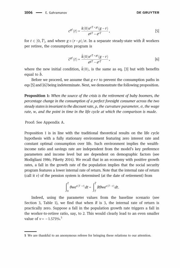
Proposition 1: When the source of the crisis is the retirement of baby boomers, thepercentage change in the consumption of a perfect foresight consumer across the twosteady states is invariant to the discount rate, ρ, the curvature parameter, σ, the wagerate, w, and the point in time in the life cycle at which the comparison is made.

Proof: See Appendix A.

Proposition 1 is in line with the traditional theoretical results on the life cyclehypothesis with a fully stationary environment featuring zero interest rate andconstant optimal consumption over life. Such environment implies the wealth-income ratio and savings rate are independent from the model’s key preferenceparameters and income level but are dependent on demographic factors (seeModigliani 1986; Piketty 2014). We recall that in an economy with positive growthrates, a fall in the growth rate of the population implies that the social securityprogram features a lower internal rate of return. Note that the internal rate of return(call it ν) of the pension system is determined (at the date of retirement) from

ðT0θweνðT − tÞdt =

ð�TTRθweνðT − tÞdt.

Indeed, using the parameter values from the baseline scenario (seeSection 3, Table 1), we find that when R is 3, the internal rate of return ispractically zero. Suppose a fall in the population growth rate triggers a fall inthe worker-to-retiree ratio, say, to 2. This would clearly lead to an even smallervalue of ν = − 1.575%.5

5 We are thankful to an anonymous referee for bringing these relations to our attention.

1006 E. Gahramanov

We now turn to a separate type of consumer – the rule-of-thumb consumer (“rot”,for short) who saves a fixed fraction, s, of his disposable wage earnings duringhis working years, and annuitizes the balance upon retirement. The agent’scapital account evolves according to the following differential equations andend-point conditions

dkðtÞdt

= rkðtÞ+ sð1− θÞw ∀t 2 ½0,T�, [7]

dkðtÞdt

= rkðtÞ−A ∀t 2 ½T, �T�, [8]

kð0Þ =0, [9]

kð�TÞ=0, [10]

where 0% ≤ s < 100% is the saving rate, and A is the constant annuity withdrawalthat eventually drives the account to zero. We show in Appendix B that

A=sð1− θÞw 1− erT

� �erðT − �TÞ − 1

∀t 2 ½T, �T�. [11]

Clearly, in the current steady-state the rule-of-thumb agent’s working lifeconsumption is

crotðtÞ= ð1− sÞð1− θÞw ∀t 2 ½0, T�, [12]

while his retirement consumption is

crotðtÞ=A+ b ∀t 2 ½T, �T�. [13]

In the new steady state, his retirement consumption will be

~crotðtÞ=A+ ~b ∀t 2 ½T, �T�, [14]

with ~crotðtÞ < crotðtÞ.

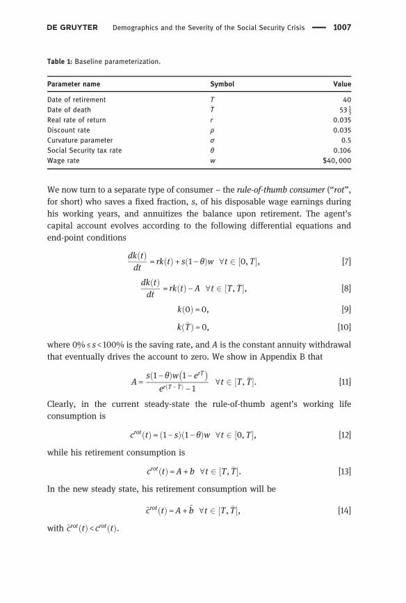
Table 1: Baseline parameterization.

Parameter name Symbol Value

Date of retirement T 40Date of death �T 53 1

3

Real rate of return r 0.035Discount rate ρ 0.035Curvature parameter σ 0.5Social Security tax rate θ 0.106Wage rate w $40, 000

Demographics and the Severity of the Social Security Crisis 1007

Proposition 2:When the source of the crisis is the retirement of baby boomers, thepercentage change in retirement consumption of the rule-of-thumb consumeracross the two steady states is invariant to time, t, and the wage rate, w, but ispositively related to the savings rate, s. Hence, the percentage drop in retirementconsumption due to a reduction in social security benefits is not as large whenmore is saved for retirement.

Proof: See Appendix C.

It should be noted the only drop in consumption experienced by the rule-of-thumbconsumer occurs during the retirement stage of life. Thus, if the consumer savedmore during their working life, he would accumulate more funds in the assetaccount, mitigating the adverse impact of the drop in the worker-to-retiree ratio.

A drop in the present value of lifetime resources due to lower pensionbenefits, causes a change in lifetime utility of the economic agent, ceterisparibus. The severity of the change might be sensitive to model parameters. Toassess a relative utility loss we, in line with Findley and Caliendo (2009), firststate the following definition.

Definition: The “compensating variation” is the constant fraction of consumptionthat has to be given to a consumer who lives in a steady state with lower pensionbenefits in order to equate his lifetime utility with the utility of an identicalconsumer receiving higher pension benefits in a different steady state.

Note that in this section we will deliberately limit our attention to the welfareanalysis of a perfect-foresight consumer, since welfare comparisons involving anon-optimizing consumer would not be straightforward. The latter issue isfurther discussed in Section 4.1.

For the perfect foresight consumer, the compensating variation, ςpf , solves

ð�T0e− ρt cpf ðtÞ� �1− σ

1− σdt =

ð�T0e− ρt

1 + ςpf� �

~cpf ðtÞ� �1− σ

1− σdt. [15]

It follows that

ςpf =kð0Þ− ~kð0Þ

~kð0Þ =θð~R−RÞ e− rT − e− r�T

� �ð1− θÞ e− rT − 1ð Þ+ ~Rθ e− r�T − e− rT

� � . [16]

Since kð0Þ > ~kð0Þ, ςpf is always positive, which is sensible.

1008 E. Gahramanov

Proposition 3: When the source of the crisis is the retirement of baby boomers, therelative welfare loss of the perfect foresight consumer is invariant to the discount rate, ρ.

Proof: Refer to eq. [16] and observe that ∂ςpf=∂ρ=0.

The natural question now to ask is whether there is a critical savings rate, s,which would make the rule-of-thumb consumer as disadvantaged as the perfectforesight consumer in terms of the relative loss in consumption. The answercritically depends on the source of the pension crisis as can be seen from thefollowing proposition and the subsequent sections.

Proposition 4: When the source of the crisis is the retirement of baby boomers,then regardless of the value of the curvature parameter, σ, the relative consump-tion losses of the rule-of-thumb and perfect foresight consumers will not be equalto each other (unless the saving rate is assumed to be s= 100%).

Proof: Using eqs [11] and [41], the equality with eq. [35] occurs only when sequals unity.

When the rule-of-thumb consumer saves his entire disposable wage throughouthis working life, his consumption loss during retirement is exactly equal to that ofthe perfect foresight agent. If we recall that the relative consumption drop for themyopic agent must monotonically decline with the saving rate, obviously a rule-of-thumb consumer cannot experience a lower percentage decline in consump-tion than a perfect foresight consumer. This would imply that the pension crisisfor the myopic agent is financially less severe.

2.2 Higher Life Expectancy vs. Retirement of Baby Boomers

We now will consider a pension crisis solely driven by an increase in lifeexpectancy. To capture the life expectancy-driven crisis, we assume a finitepopulation spread uniformly from 0 to �T years. All people die at �T, and whensomeone dies another person is born. Consequently, R=T=ð�T − TÞ. With higherlife expectancy, the finite population becomes spread from 0 to �F years (�F > �T).Thus, ~R= T=ð�F −TÞ <R.

Then, the optimal consumption profile becomes

~cpf ðtÞ= ϰð0Þer�F + gt g − rð Þeg�F − er�F

, [17]

where

Demographics and the Severity of the Social Security Crisis 1009

ϰð0Þ=ðT0e− rtð1− θÞwdt +

ð�FTe− rt~bdt. [18]

From eqs [17] and [5], the relative consumption loss of the perfect foresightagent is

Δcpf ðtÞcpf ðtÞ =

ϰð0Þ eg − rð Þ�T

− 1� �

kð0Þ e g − rð Þ�F− 1

� � − 1

=ð1− θÞ e− rT − 1

� �+ ~Rθ e− r�F − e− rT

� �ð1− θÞ e− rT − 1ð Þ+Rθ e− r�T − e− rT

� �0@

1A

×e

g − rð Þ�T− 1

e g − rð Þ�F− 1

!− 1.

[19]

Expression [19] leads to the following proposition.

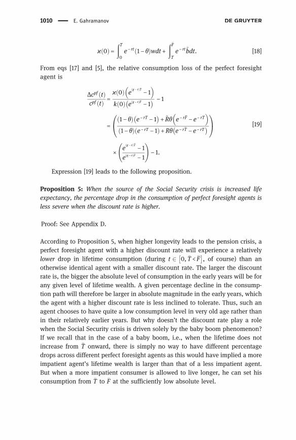
Proposition 5: When the source of the Social Security crisis is increased lifeexpectancy, the percentage drop in the consumption of perfect foresight agents isless severe when the discount rate is higher.

Proof: See Appendix D.

According to Proposition 5, when higher longevity leads to the pension crisis, aperfect foresight agent with a higher discount rate will experience a relativelylower drop in lifetime consumption (during t 2 0, �T < �F

� �, of course) than an

otherwise identical agent with a smaller discount rate. The larger the discountrate is, the bigger the absolute level of consumption in the early years will be forany given level of lifetime wealth. A given percentage decline in the consump-tion path will therefore be larger in absolute magnitude in the early years, whichthe agent with a higher discount rate is less inclined to tolerate. Thus, such anagent chooses to have quite a low consumption level in very old age rather thanin their relatively earlier years. But why doesn’t the discount rate play a rolewhen the Social Security crisis is driven solely by the baby boom phenomenon?If we recall that in the case of a baby boom, i.e., when the lifetime does notincrease from �T onward, there is simply no way to have different percentagedrops across different perfect foresight agents as this would have implied a moreimpatient agent’s lifetime wealth is larger than that of a less impatient agent.But when a more impatient consumer is allowed to live longer, he can set hisconsumption from �T to �F at the sufficiently low absolute level.

1010 E. Gahramanov

For the rule-of-thumb consumer, the new annuity withdrawal is

~A=sð1− θÞw 1− erT

� �erðT − �FÞ − 1

∀t 2 ½T, �F�, [20]

and the corresponding relative change in consumption is as follows

ΔcrotðtÞcrotðtÞ =

~A−A+ θwð~R−RÞA+Rθw

. [21]

We next establish the following two propositions.

Proposition 6: Regardless of the value of the curvature parameter, σ, percentagelosses in consumption of the rule-of-thumb consumer are equal to those of the

perfect foresight consumer if s= θðRa4 − ~RÞa5 − a4a6

, where a5 ≡ ð1− θÞ 1− erTð ÞerðT − �FÞ − 1 , a6 ≡ ð1− θÞ 1− erTð Þ

erðT − �TÞ − 1 ,

and a4 ≡ ð1− θÞ e− rT − 1ð Þ+ ~Rθ e− r�F − e− rTð Þð1− θÞ e− rT − 1ð Þ+Rθ e− r�T − e− rTð Þ

� × e

g − rð Þ�T− 1

e g − rð Þ�F− 1

� �.

Proof: See Appendix E.

Proposition 7: When the source of the Social Security crisis is the retirement ofbaby boomers, the relative loss in consumption (up to year �T) for both perfectforesight and rule-of-thumb consumers is less severe (when g =0, and s > 0%,respectively) than what it would be under a longevity-driven crisis. When g ≠0, itis unclear which type of crisis will bring a bigger consumption loss. When s=0%,the relative loss in consumption for rule-of-thumb consumers under both sources ofthe crisis is equal.

Proof: See Appendix F.

Intuitively, when a perfect foresight agent with a flat wage-consumption profilelives longer, he must smooth out his wage income over a longer horizon, and thiswill lead to a reduction in lifetime consumption (provided that wage incomeexceeds social security benefits, which is true by assumption). Thus, the consump-tion loss would be even more severe during a single period. However, with a non-flat consumption profile (g ≠0), the agent may shift his consumption loss to earlieror later stages in life. Proposition 7 also implies that when the source of the crisis isincreased life expectancy, the myopic consumer will always suffer a bigger drop inretirement consumption. The key is when everyone lives longer, the rule of thumbconsumer in question has a lower private annuity and lower benefits, whereas inthe case of the baby-boom phenomenon, he only has lower benefits with the sameprivate annuity. The lower annuity effect obviously vanishes when s=0%.

Demographics and the Severity of the Social Security Crisis 1011

Remark 1: As far as the loss in lifetime utility of the rational agent is concerned,it may be that the lifetime utility loss is not as severe. Or, perhaps the lifetimeutility change could even be positive. In a single period the relative consumptionloss may be more severe with a life expectancy-driven crisis. On the other hand,when the agent lives longer, his lifetime utility will tend to be larger becausethere are more periods being added up.

Precisely, the compensating variation for the perfect foresight consumer is now

ςpf =1− θð Þ 1− e− rT

� �+Rθ e− rT − e− r�T

� �1− θð Þ 1− e− rTð Þ+ ~Rθ e− rT − e− r�F

� �0@

1A

×e g − rð Þ�F − 1e g − rð Þ�T − 1

!e g 1− σð Þ− ρð Þ�T − 1e g 1− σð Þ− ρð Þ�F − 1

! 11− σ

− 1. [22]

Since comparative statics on eq. [22] with respect to the discount rateproduce rather cumbersome results, this time we render them to numericaldemonstrations. Nevertheless, a key conclusion from eq. [22] is that a changein discount rate does affect compensating variation for perfect foresight con-sumers. This is because when the crisis involves everyone living longer thanpreviously, it is relatively less valuable for consumers with a higher psycholo-gical discount rate to collect benefits for a longer time.

A word of caution is needed here. Based on Parfit’s idea of RepugnantConclusion, it is clear that population ageing phenomena manifested in increas-ing life expectancy and different population sizes would make welfare compar-isons a delicate ethical issue. It is problematic from an ethical viewpoint to arguethat a drop in the quality of life can be compensated by a gain in the populationsize or even length of life. There has been voluminous literature stating thatavoiding the Repugnant Conclusion is not straightforward, and experts in popula-tion ethics have long debated how to make consistent welfare comparisons insuch circumstances. Consider, for instance, switching to some kind of “averageutilitarianism” by deflating the total lifetime welfare of an agent by his corre-sponding length of life. However, suppose in the new steady state with lowerpension benefits and greater longevity we have an agent whose average utility isjust slightly lower than that in the old steady state with higher pension benefits. Isit necessarily better to have somebody live a shorter life in just a slightly bettercondition? Alternatively, in line with “critical level utilitarianism”, one mightargue that the steady state with lower pension benefits is more desirable only ifthe per period consumption level does not drop below a certain critical threshold,below which a resulting utility is negative. Yet how to determine such threshold?

1012 E. Gahramanov

Even if we determined the threshold above some individually neutral level, onecould have run into a situation where a greater number of per-period consump-tions (before a pension crisis) just below that threshold level but above the neutrallevel would have lead to more negative welfare values than a smaller number ofpost-crisis per-period consumptions (perhaps at very old ages) that are below theneutral level. This might lead to the Very Sadistic Conclusion (see Blackorby,Bossert, and Donaldson 2005; Huseby 2012). Although our paper does not aim totackle the above problems, future research is needed to investigate possibleavenues of avoiding potentially unethical conclusions.

3 Numerical Illustrations

We now simulate three separate scenarios: (1) the crisis is only triggered by thebaby-boom phenomenon; (2) the crisis is only triggered by higher life expectan-cies; and (3) the crisis is triggered jointly by (1) and (2). Table 1 shows the modelparameters.

Let the model age t =0 correspond to the actual age of 25, i.e., T =40corresponds to the retirement age of 65. The total Old-Age and SurvivorsInsurance tax rate is 10.6%, and thus we set θ=0.106, assuming that laborbears the full burden of the tax. Feigenbaum (2008) considers the curvatureparameter σ in the vicinity of 0.5, while setting the interest rate target tor =0.035, and thus we do likewise. For simplicity, assume the discount rate isequal to the interest rate, however we do vary it as seen below. We choose �T = 53 1

3

in the baseline state. We do this because the uniform population distributioncomfortably generates the current ratio of workers to retirees equal to 3.

Figure 1 plots the percentage losses in consumption of the perfect foresightand rule-of-thumb consumer for various working-age saving rates, s, and alsothe compensating variation of the perfect foresight agent. A lower value of theworker-to-retiree ratio is set at ~R= 2.

The loss in consumption of the perfect foresight agent is 1.39%, while thecompensating variation is 1.41% irrespective of the discount rate. Now, let usrefer to the scenario where greater longevity is the sole contributor to a drop inretirement benefits, which corresponds to �F = 60 (again, ~R= 2). Figure 2 reportsrelative changes in consumption and welfare.

If we set the discount rate, for example, to 6% (Figure 2(a)), the perfectforesight consumer will experience, for compatible years, only 0.88% lowerconsumption at each point across the life cycle when we compare a world withthree workers per retiree to a world with two workers per retiree. On the other

Demographics and the Severity of the Social Security Crisis 1013

hand, the myopic consumer still experiences severe consumption losses duringthe retirement phase of life. From Figure 2(b), it can be seen that the welfareeffect of the rise in dependency ratio is positive for the perfect-foresight agent,yet the higher the discount rate, the smaller the welfare gain.

3.1 A “Mixed Scenario”: Higher Longevity Coupledwith the Baby-Boom Effect

To draw more realistic quantitative results, one needs to recognize that often afall in the ratio of workers-to-retirees is triggered simultaneously by the

0% 20% 40% 60% 80% 100% 0%

5%

10%

15%

20%

25%

30%

Saving Rate

a) Consumption Loss: ρ = 6%

Perfect foresightMyopic

1% 2% 3% 4% 5% 6% 0%

5%

10%

15%

20%

25%

Discount Rate

b) Welfare Gain: ρ is relevant

Perfect foresight

Figure 2: Consumption and welfare changes due to a life expectancy-driven crisis.

0% 20% 40% 60% 80% 100% 0%

5%

10%

15%

20%

25%

30%

Saving Rate

a) Consumption Loss: ρ is irrelevant

Perfect foresightMyopic

0% 20% 40% 60% 80% 100% 0%

0.5%

1%

1.5%

2%

2.5%

3%

Discount Rate

b) Welfare Loss: ρ is irrelevant

Perfect foresight

Figure 1: Consumption and welfare changes due to a baby boom-driven crisis.

1014 E. Gahramanov

retirement of baby boomers and everyone living longer. A simple way to demon-strate the implications for such a scenario is to refer to the previous section. Itshould be noted that a new date of death can be set at some intermediate levelbetween �T = 53 1

3 and �F = 60, while a further drop in the ratio of workers toretirees can be attributed by the sudden retirement of a large number of babyboomers. We can set the new death date, �F, to 57, which means the average lifeexpectancy is up to 82 years old.6 A further decline in R will thus be assumed tocoincide with the population bubble phenomenon. Our simulation results can besummarized as follows.1) The decline of the myopic consumer’s consumption is much smaller but still

high (not lower than 17.5%) even with a moderate increase in longevity andhigh saving rates.

2) The drop in consumption of a perfect foresight agent varies greatly. It rangesfrom 10.06% (when ρ= 1%) to just 1.11% (when ρ= 6%).

3) The lifetime welfare of rational agents improves when the discount rate isrelatively low. However, when the discount rate gets even moderately high,the perfect foresight agent suffers a utility loss.

4 Extensions

4.1 Welfare Comparisons in the Presence of Rule-of-ThumbAgents

In earlier sections we focused on the welfare estimations for rational agentsonly. Technically, we could have assessed the intertemporal utility of therule-of-thumb consumers by that of perfect foresight agents as well. Although suchan approach would have been in line with some behavioral studies of pensionsystems (e.g., Feldstein 1985; Docquier 2002; İmrohoroğlu, İmrohoroğlu, and Joines2003; Hurst andWillen 2007; Cremer et al. 2008), it is certainly controversial. Giventhat individuals are not maximizing this objective, taking lifetime utility as thebenchmark would raise many objections.7

In this section, we consider an alternative approach. Let us look at the casewhere a steady lifetime consumption is the result of an optimizing model (whenr = ρ, implying g =0), and the tax rate θ is such that retirement consumption is

6 This number is close to the intermediate projections for females and males reported byTrustees in Diamond and Orszag (2005).7 We thank the Editor and an anonymous referee for bringing this point to our attention.

Demographics and the Severity of the Social Security Crisis 1015

also the same across two different agents. Thus, using expression [5] we canexpress a constant consumption profile (call it cpfconstðtÞ) as the outcome of theoptimizing model:

cpfconstðtÞ=kð0Þer�Trer�T − 1

=e− rTw erðT + �TÞð1− θÞ−RθerT − er�Tð1− θ−RθÞ

� �er�T − 1

, [23]

where the tax rate shall be chosen so that eq. [23] equals eq. [13]. After somealgebra, we can show that such a social security tax rate must be equal to

θ=er�T − erTð1− sÞ − erðT + �TÞs

er�Tð1 +RÞ− erðT + �TÞs− erTð1 +R− sÞ . [24]

Substituting eq. [24] into eq. [23], we obtain

cpfconstðtÞ=Rwð1− sÞðerT − er�TÞ

− er�Tð1 +RÞ+ erTð1 +R− sÞ+ erðT + �TÞs. [25]

Expression [25] is a function of a constant saving rate, s, so that for anyvalue of s, there is a flat, perfect-foresight consumption path, where the corre-sponding consumption rate is equal to that of the rule-of-thumb agent with thesaving rate s. Consequently, we obtain the percentage change in consumptiondue to a rise in the dependency ratio:

ΔcpfconstðtÞcpfconstðtÞ

=ðR− ~RÞðer�T + erTðs− 1Þ− erðT + �TÞsÞ

Rð− er�Tð1 + ~RÞ+ erTð1 + ~R− sÞ+ erðT + �TÞsÞ . [26]

So, the optimizing, “constant saving-rule” consumer’s compensating varia-tion (ςpfconst) is

ςpfconst =ðR− ~RÞðer�T + erTðs− 1Þ− erðT + �TÞsÞ

~Rðer�Tð1 +RÞ− erðT + �TÞs+ erTðs−R− 1ÞÞ . [27]

Figure 3 plots the compensating variation, against a range of possible savingrates.8

We see that a higher (optimal, yet constant) saving rule implies the utilityloss is lower due to a shortfall of pension benefits. Yet an important implicationfor welfare analysis is that seemingly myopic rule-of-thumb behavior can in fact

8 We can evaluate eq. [27] for various saving rates. However, for every saving rate, the payrolltax rate given by eq. [24] gets automatically updated. These different tax rates for the differentsteady-state comparisons are not problematic because we would keep the tax rates constantacross the steady states. Since θ should not fall outside the 0% and 100% region, we have tolimit the range of the saving rate, s, we can use.

1016 E. Gahramanov

be an outcome of a well-defined (however unconventional) optimizing model.Thus, more empirical research is needed to determine the realism of the objec-tive function in such models. Doing so might greatly aid researchers to under-take consistent and plausible welfare analysis.

4.2 Cases of Changing Cohort Sizes and Retirement Ages

In this section, we look at a scenario with changing cohort sizes, and we alsoconsider retirement age increases in such a way as to hold the dependency ratioconstant despite higher life expectancy.9 We start by assuming that at eachinstant in time a new cohort replaces an old cohort, yet the size of each cohortgrows exponentially at the rate n > 0. It is straightforward to show that thedependency ratio will depend on n (see also Piketty 2014 on this), and so longas n is constant, the worker-to-retiree ratio will also be constant.

We can further find that for any higher life length �F (�F > �T), the retirement date,which ensures the same worker-to-retiree ratio as before (call it F), is given by

0% 2% 4% 6% 8% 10% 0%

5%

10%

Optimal (Constant) Saving Rate

Welfare Loss

Figure 3: Welfare changes of optimizing “constant saving-rule” agents.

9 We thank an anonymous referee for suggesting to investigate this scenario.

Demographics and the Severity of the Social Security Crisis 1017

F = �FT�T. [28]

Consequently, the present value of lifetime income for the perfect foresightagent becomes

ϰð0Þnew =ðF0e− rtð1− θÞwdt +

ð�FFe− rtbdt, [29]

where superscript “new” indicates the situation, where an increase in longevityis accompanied by an increase in the retirement age from T to F = �FT=�T, so thatstill b=Rθw. Thus, the corresponding consumption profile becomes

~cpf ðtÞnew = ϰð0Þnewer�F + gt g − rð Þeg�F − er�F

. [30]

From eqs [30] and [5], the relative consumption change of the perfect fore-sight agent is

Δcpf ðtÞcpf ðtÞ =

ϰð0Þnew eg − rð Þ�T

− 1� �

kð0Þ e g − rð Þ�F− 1

� � − 1

=ð1− θÞ e− rF − 1

� �+Rθ e− r�F − e− rF

� �ð1− θÞ e− rT − 1ð Þ+Rθ e− r�T − e− rT

� �0@

1A

×e

g − rð Þ�T− 1

e g − rð Þ�F− 1

!− 1.

[31]

Proposition 8: ϰð0Þnew > kð0Þ.

Proof: See Appendix G.

However, it is still not clear whether eq. [31] is positive because term eg − rð Þ�T

− 1 is lessin an absolute sense than term e

g − rð Þ�F− 1. Let us suppose r =0.035, σ = 1.1, ρ=0.02,

θ=0.106, w= 1, �T = 53 13,

�F = 57, T =40. Thus, R= 3, F = 42.75. Clearly,~R= F=ð�F − FÞ= 3 =R, i.e., ~b= b. As a result, ϰð0Þnew = 20.6212, whilekð0Þ= 20.0796. We obtain cpf ðtÞ=0.630854e0.0136364t, and ~cpf ðtÞnew =0.625685e0.0136364t, respectively. Thus, we observe a decline in the lifetime consump-tion path for comparable ages. However, let us raise the discount rate to ρ=0.03.Then cpf ðtÞ=0.761595e0.00454545t, and ~cpf ðtÞnew =0.762369e0.00454545t, respectively.Thus, we observe a rise in the lifetime consumption path. Intuitively, when thediscount rate is relatively high, consumption in older age is low anyway, meaningthat an extra gain in the years of life at old age does not require many resources tosupport late life consumption, thus allowing greater consumption overall.

1018 E. Gahramanov

Remark 2: Applying the reasonings used in Appendix D, it is not difficult todeduce from eq. [31], that the percentage drop in the consumption of perfectforesight agents would be less pronounced when the discount rate is higher.

Similarly, we can obtain the new annuity withdrawal for the rule-of-thumb agent as

~Anew =sð1− θÞw 1− erF

� �erðF − �FÞ − 1

∀t 2 ½F, �F�, [32]

and the corresponding relative change in post-retirement consumption is asfollows

ΔcrotðtÞcrotðtÞ =

~Anew

−AA+Rθw

. [33]

Proposition 9: ~Anew >A, implying that when the longevity increase is associatedwith a sufficient rise in the retirement age so the dependency ratio is heldconstant, the rule-of-thumb agents’ consumption actually increases.

Proof: See Appendix H.

Intuitively, continuous compounding provides exponential growth of the myopicagent’s financial account over a longer period of working life, and when theagent finally retires, he can afford greater annuity amount withdrawal over asomewhat longer retirement span. Thus, ~Anew >A, and because the same amountof pension benefit is now preserved over the retirement span, the rule-of-thumbagent’s retirement consumption is greater.

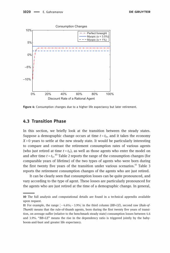
Given that our myopic agent unequivocally obtains a gain in his post-retire-ment consumption under the present scenario, let us see what the discount rate ofthe perfect-foresight consumer should be so the latter receives at least the sameconsumption gain. Suppose the saving rate, s, is equal to 3.5%, which is consistentwith the estimates in Thaler and Benartzi (2004). Using the same parameter valuesas in Table 1, as well as �F = 57 and F = 42.75, we plot the percentage gain in theconsumption of myopic agents, and the percentage changes of lifetime consump-tion of rational agents under different discount rates.

When the saving rate is mildly high, no matter how impatient the rationalagent is, his maximum consumption gain is lower than that of the myopic agent.Yet if we drop s to 1%, relatively impatient rational agents experience biggerconsumption gain. Figure 4 also shows rational agents with very low discountrate will actually experience a big consumption loss.

Demographics and the Severity of the Social Security Crisis 1019

4.3 Transition Phase

In this section, we briefly look at the transition between the steady states.Suppose a demographic change occurs at time t = t0, and it takes the economyX > 0 years to settle at the new steady state. It would be particularly interestingto compare and contrast the retirement consumption rates of various agents(who just retired at time t = t0), as well as those agents who enter the model onand after time t = t0.

10 Table 2 reports the range of the consumption changes (forcomparable years of lifetime) of the two types of agents who were born duringthe first twenty five years of the transition under various scenarios.11 Table 3reports the retirement consumption changes of the agents who are just retired.

It can be clearly seen that consumption losses can be quite pronounced, andvary according to the type of agent. These losses are particularly pronounced forthe agents who are just retired at the time of a demographic change. In general,

0% 20% 40% 60% 80% 100%

–10%

–5%

0%

5%

10%

Discount Rate of a Rational Agent

Consumption Changes

Perfect foresightMyopic (s = 3.5%)Myopic (s = 1%)

Figure 4: Consumption changes due to a higher life expectancy but later retirement.

10 The full analysis and computational details are found in a technical appendix availableupon request.11 For example, the range ½− 4.6%;− 3.9%� in the third column (BB+LE), second raw (Rule-of-Thumb) means that the rule-of-thumb agents, born during the first twenty five years of transi-tion, on average suffer (relative to the benchmark steady state) consumption losses between 4.6and 3.9%. “BB+LE” means the rise in the dependency ratio is triggered jointly by the baby-boom-and-bust and greater life expectancy.

1020 E. Gahramanov

we find the magnitude of the changes are quite sensitive to the parameterizationused, meaning that a standard steady state comparison should be contrastedwith a more complicated transition analysis. Doing so would enable a richer setof results to be obtained, yet it would certainly add an additional layer ofanalytical and computational complexity in trying to project future consumptionpatterns for the elderly in the immediate, as well as distant future.

5 Conclusion

There is widespread sentiment among business and policy analysts that givenpopulation ageing, more elderly people would mean more old-age consumption,and thus huge business opportunities. In this paper, we look at a micro-levelanalysis of intertemporal consumption/saving behavior, and find that in thepresence of heterogeneity with respect to the levels of impatience, as well ashow closely consumers follow a neoclassical model of spending, different demo-graphic challenges might imply greatly varied consumption changes at old age.For instance, we find that a baby-boom-and-bust phenomenon would generallylead to significant consumption losses for rule-of-thumb consumers, and theselosses can be assumed to be low only when an individual savings rate is veryhigh. In addition, while in a baby-boom-and-bust phenomenon, impatience het-erogeneity plays no role in quantifying a perfect-foresight consumer’s spendingchanges, however it does so if one assumes an increase in longevity. For example,if one assumes everyone is very impatient, then a shortfall in pension benefitswould lead to a moderate decline in per-period consumption of a rational agent,yet still leads to very low spending levels at very old age. In contrast, a rule-of-

Table 3: Consumption changes for those who are just retired at the time of the shock, ρ=3.5%,s=3.5%.

BB only LE only BB+LE LE+High Ret.

Perfect-foresight − 13.0% − 28.0% − 22.8% −9.8%Rule-of-Thumb − 18.3% − 30.0% − 25.9% − 7.2%

Table 2: Consumption changes for those born after the shock, ρ=3.5%, s=3.5%.

BB only LE only BB+LE LE+High Ret.

Perfect-foresight ½− 5.7%;−4.3%� ½− 7.5%;−6.4%� ½−6.8%;− 5.5%� ½− 3.0%;− 1.9%�Rule-of-Thumb ½− 3.0%;− 2.3%� ½− 5.5%;−4.8%� ½−4.6%;− 3.9%� ½−4.4%;5.0%�

Demographics and the Severity of the Social Security Crisis 1021

thumb consumer would suffer larger consumption losses. However, these losseswould turn into gains if one models a policy response where an increase inlongevity is matched by a proportional increase in the retirement age in order topreserve the current benefit levels. But if so, perfect foresight consumers wouldexperience, for many years during the old age, a big consumption loss or mod-erate consumption gain depending on how impatient they are. We also touchupon the issues of welfare analysis and transitional comparisons, and discuss theassociated complexities and challenges. We suggest future research also focus onthe interaction of household behavior and resulting sectoral demand at theaggregate level. We hope by identifying (via surveys and empirical studies) thedistribution of the core consumer types, accounting for some of the key behavioraland psychological differences among the consumers, while focusing on theirmicro-level decisions in the context of demographic phenomena, will aid policy-makers and business circles in their future projections.

Acknowledgments: I thank Johann Brunner and two anonymous referees fortheir very helpful comments. I would also like to thank Frank Caliendo and ScottFindley for many helpful discussions and encouragement. All errors are my own.

Appendix A

Using eqs [5] and [6], we obtain the percentage change in consumption of theperfect foresight agent:

Δcpf ðtÞcpf ðtÞ ≡ ~cpf ðtÞ− cpf ðtÞ

cpf ðtÞ =~kð0Þ− kð0Þ

kð0Þ . [34]

Integrate out kð0Þ and ~kð0Þ, and substitute into eq. [34] to get

θð~R−RÞ e− r�T − e− rT� �

ð1− θÞ e− rT − 1ð Þ+Rθ e− r�T − e− rT� � . [35]

Expression [35] is invariant to ρ, σ, w and t.

Appendix B

The general solution to differential equation [7] is

kðtÞ = −sð1− θÞw

r+ z1ert, [36]

1022 E. Gahramanov

where z1 is constant. Using the initial solution kð0Þ=0, a particular solution is

kðtÞ= sð1− θÞwr

ert − 1� �

, [37]

which implies

kðTÞ= sð1− θÞwr

erT − 1� �

. [38]

The general solution to differential equation [8] is

kðtÞ= Ar+ z2ert, [39]

where z2 is constant. Using the boundary condition kð�TÞ=0, a particular solution is

kðtÞ= Ar

1− erðt − �TÞ� �

. [40]

Finally, we obtain eq. [11] by setting t equal to T in eq. [40], and then equatingeqs [40] and [38] to solve for A.

Appendix C

Using eqs [13] and [14], we obtain

ΔcrotðtÞcrotðtÞ ≡ ~crotðtÞ− crotðtÞ

crotðtÞ =θw ~R−R� �

A+Rθw∀t 2 ½T, �T�. [41]

Since A is proportional to w, the wage rate can be factored out and eliminated

from eq. [41]. Since ∂A=∂s > 0 and ~R−R < 0, then ∂ΔcrotðtÞcrotðtÞh i

=∂s > 0.

Appendix D

Partially differentiating eq. [19] with respect to ρ, reveals the sign of comparativestatics depends on the sign of

∂g∂ρ

�Teg − rð Þ�T

eg − rð Þ�F

− 1� �

− �Feg − rð Þ�F

eg − rð Þ�T

− 1� �� �

e g − rð Þ�F− 1

� �2 . [42]

As ∂g=∂ρ < 0, expression [42] is negative when

�T eg − rð Þ�F

− 1� �

eg − rð Þ�T

> �Feg − rð Þ�F

eg − rð Þ�T

− 1� �

. [43]

Demographics and the Severity of the Social Security Crisis 1023

For cases g > r or g < r, expression [43] can be restated as

�Teg − rð Þ�T

e g − rð Þ�T− 1

>�Fe

g − rð Þ�F

e g − rð Þ�F− 1

. [44]

For eq. [44] to hold, the derivative of the left-hand side of eq. [44] with respect to�T must be negative, or

g − rð Þ�T + 1 > eg − rð Þ�T

, [45]

which cannot be true. Hence, eq. [42] is positive.

Appendix E

First, rewrite eq. [21] as

~A+ ~RθwA+Rθw

− 1≡ a5s+ ~Rθa6s+Rθ

− 1. [46]

Now, note that eq. [19] can be compactly stated as

a4 − 1. [47]

Finally, equate eqs [46]–[47] and solve for the unique, critical savings rate toconfirm the proposition.

Appendix F

For the perfect foresight consumer with g =0, we start comparingϰð0Þ e

− r�T− 1

� �kð0Þ e− r�F

− 1� � − 1

(modified expression [19]) with~kð0Þ− kð0Þ

kð0Þ (expression [34]). Observe the latter is

always negative. Hence, all we have to do is to prove modified eq. [19] is lessthan eq. [34]. Thus, we require

ϰð0Þ e− r�T − 1� �

kð0Þ e− r�F − 1� � <

~kð0Þkð0Þ . [48]

Multiplying both sides of eq. [48] by kð0Þ e− r�F − 1� �

, integrating-out ϰð0Þ and~kð0Þ, and collecting terms, finally produces the following inequality:

ð1− θÞw e− r�T − e− rðT + �TÞ − e− r�F + e− rðT + �FÞ� �

> ~b e− r�T − e− rðT + �TÞ − e− r�F + e− rðT + �FÞ� � [49]

1024 E. Gahramanov

We can divide both sides of eq. [49] by the bracketed expression. However first,we have to find out whether the expression is negative in sign.

Now, we rewrite the expression as Λ1 −Λ2, where Λ1 ≡ e− r�T − e− rðT + �TÞ, and

Λ2 ≡ e− r�F − e− rðT + �FÞ. Note that Λ1 > 0. We also observe that Λ2 is the same as Λ1,

but the only difference is �T is replaced by �F. Since the latter is strictly greater

than the former, all we need to know is how increasing �T changes the value of

Λ1. Clearly, ∂Λ1=∂�T = r e− rðT + �TÞ − e− r�T� �

is negative. Thus, Λ1 >Λ2, meaning that

expression [49] collapses to ð1− θÞw > ~b (( ð1− θÞw > b), which is true byassumption.

Now we consider the case when g < 0 (or, r < ρ). Using eqs [34] and [19], weneed to prove that

ϰð0Þ eg − rð Þ�T

− 1� �

kð0Þ e g − rð Þ�F− 1

� � <~kð0Þkð0Þ . [50]

The latter inequality is the same as

ϰð0Þ eg − rð Þ�T

− 1� �

> ~kð0Þ eg − rð Þ�F

− 1� �

, [51]

or

~Rwθ e− rT − e− r�F� �

+wð1− θÞe− rT erT − 1� �� �

eg − rð Þ�T

− 1� �

> ~Rwθ e− rT − e− r�T� �

+wð1− θÞe− rT erT − 1� �� �

eg − rð Þ�F

− 1� �

[52]

When g < 0, the term eg − rð Þ�F

− 1� �

is more negative than the term eg − rð Þ�T

− 1� �

.

However, the term ~Rwθ e− rT − e− r�F� �

is positive but greater than the term

~Rwθ e− rT − e− r�T� �

. Thus, eq. [52] may or may not hold. We clearly achieve the

same sort of ambiguity in general when g > 0.

Finally, for the rule-of-thumb consumer, compare eq. [21] with eq. [41]. Notethat when s > 0, ~A <A (when s=0, ~A=A=0). The proof then follows.

Appendix G

Suppose

kð0Þ − ϰð0Þnew ≥0. [53]

Rewrite the left-hand-side of eq. [53] as

Demographics and the Severity of the Social Security Crisis 1025

− Rwθ eFr +�Fr + rT − eFr + rT + r�T

� �+ wð1− θÞ −Rwθð Þ eFr +

�Fr + r�T − e�Fr + rT + r�T

� �� �

×e− Fr − �Fr − rT − r�T

r, [54]

or, as

Rwθ eFr +�Fr + rT − eFr + rT + r�T

� �+ wð1− θÞ −Rwθð Þ eFr +

�Fr + r�T − e�Fr + rT + r�T

� �≤0. [55]

The latter cannot be true since by assumption, wð1− θÞ >Rwθ, while �F > �T,and F >T. Thus, ϰð0Þnew > kð0Þ.

Appendix H

Let β≡ �F=�T. From eq. [28], we then have F = βT, while �F = β�T. Thus, eq. [32] canbe restated as

~Anew =sð1− θÞw 1− eβrT

� �eβrðT − �TÞ − 1

. [56]

Since β > 1, eq. [56] implies that going from A (see expression [11]) to ~Anew issimilar to increasing r. Thus, we can simply differentiate eq. [11] with respect to rto check its sign. We have

∂A∂r

= erðT − �TÞsð1− θÞwT er�T − 1� �

− �T erT − 1� �� �

ðerðT − �TÞ − 1Þ2. [57]

Clearly, eq. [57] is positive if T er�T − 1� �

− �T erT − 1� �

is, and the latter indeed is

greater than zero.12 Therefore, ~Anew exceeds A.

References

Abdel-Ghany, M., and D. L. Sharpe. 1997. “Consumption Patterns among the Young-Old andOld-Old.” The Journal of Consumer Affairs 31 (1):90–112.

Blackorby, C., W. Bossert, and D. J. Donaldson. 2005. Population Issues in Social Choice Theory,Welfare Economics, and Ethics. Cambridge: Cambridge University Press.

12 The proof is omitted for the sake of brevity, but is straightforward and available uponrequest.

1026 E. Gahramanov

Boyle, M. 2013. “Aging Boomers Stump Marketers Eyeing $15 Trillion Prize.” BloombergBusiness (September 17).

Bradshaw, D. 2015. “Ageing Population in China Creates Business Opportunities.” The FinancialTimes Limited (March 29).

Brunner, J. K. 2002. “Welfare Effects of Pension Finance Reform.” Johannes Kepler University ofLinz Working Paper.

Campbell, J. Y., and N. Gregory Mankiw. 1989. “Consumption, Income and Interest Rates:Reinterpreting the Time Series Evidence.” In NBER Macroeconomics Annual 1989, editedby O. J. Blanchard and S. Fischer, 185–216. Cambridge, MA: MIT Press.

Campbell, J. Y., and N. Gregory Mankiw. 1990. “Permanent Income, Current Income, andConsumption.” Journal of Business and Economic Statistics 8 (3):265–79.

Cremer, H., P. De Donder, D. Maldonado, and P. Pestieau. 2008. “Designing a Linear PensionScheme with Forced Savings and Wage Heterogeneity.” International Tax and PublicFinance 15 (5):547–62.

Diamond, P. A., and P. R. Orszag. 2005. Saving Social Security: A Balanced Approach, RevisedEdition. Washington, D.C.: The Brookings Institution.

Docquier, F. 2002. “On the Optimality of Public Pensions in an Economy with Life-Cyclers andMyopes.” Journal of Economic Behavior and Organization 47 (1):121–40.

Feigenbaum, J. 2008. “Can Mortality Risk Explain the Consumption Hump?” Journal ofMacroeconomics 30 (3):844–72.

Feigenbaum, J., F. Caliendo, and E. Gahramanov. 2011. “Optimal Irrational Behavior.” Journal ofEconomic Behavior and Organization 77 (3):285–303.

Feigenbaum, J., E. Gahramanov, and X. Tang. 2013a. “Is It Really Good to Annuitize?” Journal ofEconomic Behavior and Organization 93:116–40.

Feigenbaum, J., E. Gahramanov, and X. Tang. 2013b. “Can High Discount Rates Increase CapitalAccumulation?” Utah State University Working Paper.

Feldstein, M. 1985. “The Optimal Level of Social Security Benefits.” Quarterly Journal ofEconomics 100 (2):303–20.

Findley, S. T., and F. Caliendo. 2007. “OutSMarTing the Social Security Crisis.” Public FinanceReview 35 (6):647–68.

Findley, S. T., and F. N. Caliendo. 2009. “Short Horizons, Time Inconsistency, and OptimalSocial Security.” International Tax and Public Finance 16 (4):487–513.

Findley, S. T., and F. N. Caliendo. 2010. “Does It Pay to Be SMarT?” Journal of PensionEconomics and Finance 9 (3):321–44.

Hurst, E., and P. Willen. 2007. “Social Security and Unsecured Debt.” Journal of PublicEconomics 91 (7–8):1273–97.

Huseby, R. 2012. “Sufficiency and Population Ethics.” Ethical Perspectives19 (2):187–206.

İmrohoroğlu, A., S. İmrohoroğlu, and D. H. Joines. 2003. “Time-Inconsistent Preferences andSocial Security.” Quarterly Journal of Economics 118 (2):745–84.

Kaplow, L. 2006. “Myopia and the Effects of Social Security and Capital Taxation on LaborSupply.” NBER Working Paper No. 12452.

Kronenberg, T. 2009. “The Impact of Demographic Change on Energy Use andGreenhouse Gas Emissions in Germany.” Ecological Economics 68 (10):2637–45.

Lacomba, J. A., and F. Lagos. 2006. “Population Ageing and Legal Retirement Age.” Journal ofPopulation Economics 19 (3):507–19.

Demographics and the Severity of the Social Security Crisis 1027

Lusardi, A. 1999. “Information, Expectations, and Savings for Retirement.” In BehavioralDimensions of Retirement Economics, edited by H. Aaron, 81–115. Washington, DC:Brookings Institution Press and Russell Sage Foundation.

Modigliani, F. 1986. “Life Cycle, Individual Thrift, and the Wealth of Nations.” AmericanEconomic Review 76 (3):297–313.

NSW Government. 2012. NSW Ageing Strategy. Sydney: Department of Family and CommunityServices, Office for Ageing.

Piketty, T. 2014. “Economics of Inequality.” Paris School of Economics Lecture Notes.Thaler, R. H. 1994. “Psychology and Savings Policies.” American Economic Review

84 (2):186–92.Thaler, R. H., and S. Benartzi. 2004. “Save More TomorrowTM: Using Behavioral Economics to

Increase Employee Saving.” Journal of Political Economy 112 (1):S164–S187.The Rockefeller Foundation. 2014. Rockefeller Millennials Survey. Global Strategy Group.Wong, W.-K. 2012. “Consumption Response to Government Transfers: Behavioral Motives

Revealed by Savers and Spenders.” Contemporary Economic Policy 30 (4):489–501.

1028 E. Gahramanov