On the decline of biodiversity due to area lossstorch/publications/Keil_Storch_Jetz...On the decline...

ARTICLE

Received 27 Apr 2015 | Accepted 9 Oct 2015 | Published 17 Nov 2015

On the decline of biodiversity due to area lossPetr Keil1,2, David Storch2,3 & Walter Jetz1

Predictions of how different facets of biodiversity decline with habitat loss are broadly

needed, yet challenging. Here we provide theory and a global empirical evaluation to address

this challenge. We show that extinction estimates based on endemics–area and backward

species–area relationships are complementary, and the crucial difference comprises the

geometry of area loss. Across three taxa on four continents, the relative loss of species, and

of phylogenetic and functional diversity, is highest when habitable area disappears inward

from the edge of a region, lower when it disappears from the centre outwards, and lowest

when area is lost at random. In inward destruction, species loss is almost proportional to area

loss, although the decline in phylogenetic and functional diversity is less severe. These trends

are explained by the geometry of species ranges and the shape of phylogenetic and functional

trees, which may allow baseline predictions of biodiversity decline for underexplored taxa.

DOI: 10.1038/ncomms9837 OPEN

1 Department of Ecology and Evolutionary Biology, Yale University, 165 Prospect Street, New Haven, Connecticut 06520-8106, USA. 2 Center for TheoreticalStudy, Jilska 1, 110 00, Prague 1, Czech Republic. 3 Department of Ecology, Faculty of Science, Charles University, Vinicna 7, 128 44, Prague 2, Czech Republic.Correspondence and requests for materials should be addressed to P.K. (email: [email protected]).

NATURE COMMUNICATIONS | 6:8837 | DOI: 10.1038/ncomms9837 | www.nature.com/naturecommunications 1

& 2015 Macmillan Publishers Limited. All rights reserved.

mailto:[email protected]

http://www.nature.com/naturecommunications

Habitat loss due to accelerated climate change and directhuman impact has been causing a decline of biodiversityand associated ecosystem services1–3. Direct estimates of

biodiversity loss are challenging because of highly incompleteglobal species’ distribution knowledge4 and the difficulties ofascertaining actual extinctions5–7. Instead, estimates of diversityloss have relied on indirect methods, such as the relationshipbetween area and the number of species in that area, the species–area relationship (SAR)8–11, or the relationship between an areathat is lost and the number of species confined to it, theendemics–area relationship (EAR)12,13.

Recently, He and Hubbell12 initiated discussion over thereliability of the indirect methods, claiming that the SAR-basedmethod (also known as backward estimation) overestimatesextinctions when compared with the EAR-based method(forward estimation). This debate has generated several valuableinsights, such as recognition that EAR and SAR are linked by thecomplementarity of area that is lost and the area that remains14,recognition of point reflection symmetry of the two curves13, oridentification of critical role of aggregation of individuals15 andecological context16,17 at small-scale plots. However, this debatehas not yet been settled, and there are still critical unresolvedissues, as well as opportunities for synthesis.

Specifically, it has been suggested that different spatialarrangements of habitat loss lead to different extinctionestimates18–21, which follows implicitly from comparingestimates of the forward and backward methods8,12,16. Theemerging pattern has been that, given the same amount of losthabitable area, inward area loss starting on the edges of a regionleads to higher average proportional loss of species richness thanwhen area is lost outward from within the centre of the region.Yet, it is unclear if such pattern is inevitable, that is, if there is atheoretical possibility that, contrary to He and Hubbell’s claim12,SARs (the backward method) can also actually underestimateextinction rates. Further, apart from the anecdotal case of USbirds12, this discrepancy has been demonstrated, and explainedby aggregation of individuals15, only at small scales. It isunknown if the discrepancy holds at continental to globalscales, and if it holds, what generates it. These scales are critical,as the whole species’ ranges are lost at such large scales, and theextinctions are thus irreversible. Also, it is the global scale atwhich the current high-profile debate on the magnitude ofdiversity loss (that is, extinction crisis) takes place5,22. In contrast,studies of diversity loss with area loss have been mostly confinedto local plots12, which have conservation relevance in localcontext, but are irrelevant for global estimates (see Supplementary

Note 1 for details). In addition, both the existing theory andempirical assessments of diversity loss under area loss havetraditionally comprised only the number of species, discountingoften highly variable evolutionary and functional uniqueness ofspecies23.

Here we overcome these limitations by explicitly addressinghow the spatial configuration of area loss affects the loss ofspecies, and of associated phylogenetic diversity (PD) andfunctional diversity (FD)24,25. In the first part, we advance thetheoretical basis for the estimation of the decline of taxonomic,phylogenetic and functional diversity due to area loss, withparticular emphasis on geometry of the area loss. We thenempirically address these issues using data on three majorvertebrate taxa in nine large-scale regions and three geometries ofarea loss: contiguous inward, outward and randomly scattered.We further relate the magnitude of diversity loss to predictorssuch as mean range size, range clumpedness and shape. We showthat the commonly used extinction estimates based purely on arealoss are misleading at large scales—the direction of the area loss iscrucial, with a contiguous area loss coming from the edges ofregions inwards being, on average, the most serious threat tobiodiversity. Second, the direction of area loss is consistentlymore important for extinction estimates than mean species rangesize. Third, PD and FD are more resistant to loss of area thanspecies richness. Finally, we show how this resistance is related totaxon-wide estimates of phylogenetic and functional similarity.

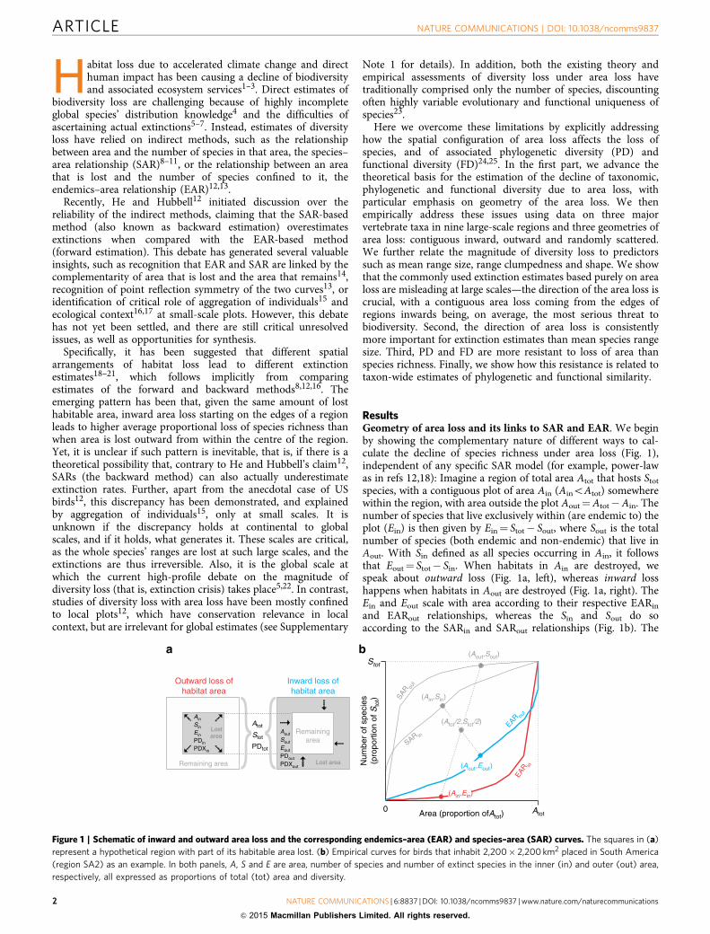
ResultsGeometry of area loss and its links to SAR and EAR. We beginby showing the complementary nature of different ways to cal-culate the decline of species richness under area loss (Fig. 1),independent of any specific SAR model (for example, power-lawas in refs 12,18): Imagine a region of total area Atot that hosts Stot

species, with a contiguous plot of area Ain (AinoAtot) somewherewithin the region, with area outside the plot Aout¼Atot�Ain. Thenumber of species that live exclusively within (are endemic to) theplot (Ein) is then given by Ein¼ Stot� Sout, where Sout is the totalnumber of species (both endemic and non-endemic) that live inAout. With Sin defined as all species occurring in Ain, it followsthat Eout¼ Stot� Sin. When habitats in Ain are destroyed, wespeak about outward loss (Fig. 1a, left), whereas inward losshappens when habitats in Aout are destroyed (Fig. 1a, right). TheEin and Eout scale with area according to their respective EARin

and EARout relationships, whereas the Sin and Sout do soaccording to the SARin and SARout relationships (Fig. 1b). The

PDXin

Outward loss ofhabitat area

Remaining area

Ain

Sin

Ein

PDin

PDXin

Inward loss ofhabitat area

Aout

Sout

Eout

PDout

PDXout

Remainingarea

0

SAR in

EAR in

EAR out

SAR ou

t

Atot

Stot

Area (proportion ofAtot)

Num

ber

of s

peci

es(p

ropo

rtio

n of

Sto

t) (Ain,Sin)

(Ain,Ein)

(Aout,Sout)

(Aout,Eout)

(Atot/2,Stot/2)Atot

Stot

PDtot

Lost area

Lostarea

Figure 1 | Schematic of inward and outward area loss and the corresponding endemics–area (EAR) and species–area (SAR) curves. The squares in (a)

represent a hypothetical region with part of its habitable area lost. (b) Empirical curves for birds that inhabit 2,200� 2,200 km2 placed in South America

(region SA2) as an example. In both panels, A, S and E are area, number of species and number of extinct species in the inner (in) and outer (out) area,

respectively, all expressed as proportions of total (tot) area and diversity.

ARTICLE NATURE COMMUNICATIONS | DOI: 10.1038/ncomms9837

2 NATURE COMMUNICATIONS | 6:8837 | DOI: 10.1038/ncomms9837 | www.nature.com/naturecommunications



EARin thus follows a point reflection symmetry with SARout andanalogically EARout is symmetrical to SARin (ref. 13).

Assuming immediate extinction (that is, no extinction debt),relevant for extinction estimates are always the EAR curves,which we also call extinction curves. The number of extinctspecies can be calculated directly from the EAR for the lost area,or indirectly by rotating the SAR for the remaining area on itsaxis about a central point14,26 (Fig. 1b); the latter being analogousto the backward method of estimating extinctions. The backwardapproach was considered incorrect by He and Hubbell12, butrecognized as valid by others14,27, with differences from theforward (that is, direct or EAR-based) method arising fromdiffering geometries of area loss. Specifically, in the case ofcontiguous area loss, the forward (EAR-based) method representsarea loss that goes outward from within, whereas the backward(SAR-based) method corresponds to inward loss starting from theedges of a region14.

Theoretical predictions. How severely diversity declines witharea loss is reflected by steepness of EAR extinction curves, whichin turn is determined by both the spatial arrangement of indivi-dual species ranges26 and of area loss. Using four distinct modelsof range placement (see Methods and Fig. 2 for details) and threescenarios of area loss in both analytical and simulation settings(Fig. 2), we make the following predictions:

Assuming random placement of discontinuous scattered ranges(Model 1; Fig. 2a), the inward and outward extinction curvesshould overlap; this coincidence of forward and backward curvesfor the randomly placed non-contiguous ranges stems from thesame causes as the coincidence of complementary SAR, nestedSAR and non-nested SAR for the random spatial distribution ofindividuals described by refs 12,15.

Assuming non-random concentration of contiguous ranges inone part of the region (Model 2; Fig. 2b), trivial and predictabledifferences should emerge between the inward and outwardEARs—when ranges are packed by the edges of the region(Fig. 2b) they will obviously be removed first by the inward arealoss, and the opposite holds for ranges concentrated in the middleof the region. However, differences between EARin and EARout

also emerge from models of random range placement (see below),so the difference is not just an issue of range concentration inparticular regions.

Assuming random placement of contiguous ranges (Models 3and 4, Fig. 2c,d and Supplementary Fig. 4), that is, when rangeswithin a region are distributed randomly and are convex andcontiguous geometrical shapes, non-trivial differences betweenEARin and EARout emerge because of the different ways therandomness is modelled. For analytical arguments, we usecircular ranges in a circular region (Fig. 2e–g; here we wereinspired by ref. 28), whereas for simulation purposes (Fig. 2a–d)we use rectangular ranges on a rectangular grid.

Let us have a circular region of area Atot and radius rtot, dividedinto an outer domain of area Aout and an inner domain of area Ain

with radius rin (Fig. 2e). Imagine that either Ain or Aout arecompletely destroyed, causing the loss of Ein or Eout. Let us setAin¼Aout¼Atot/2, and hence rin¼ rtot/

ffiffiffi2p

; in such case we are inthe middle of the extinction curve (Fig. 1b), and any differencebetween Ein and Eout is due to reasons other than AinaAout.Now when we try to place a circular range of radius rr (Fig. 2e)at a random location within the region, we realize thatthere are actually several ways to model such random placement26.Here we consider two most distinct ones, and call them Models3 and 4:

In Model 3 the whole range is placed randomly, so that itsentire body must fall within the region boundary, which causes

the well-known mid-domain effect29 (Fig. 2c and SupplementaryFig. 4a). Of key interest is the probability Pout that the range fallsexclusively (entirely) within the outer domain, contributing toEout, and probability Pin that the range will fall exclusively withinthe inner domain, contributing to Ein. These probabilities are(see Supplementary Note 2 for further details):

Pout ¼1; if rin ¼ 0

0; if rr � rtot� rinð Þ=2Xout; if rro rtot� rinð Þ=2;

8<: ð1Þ

where

Xout ¼rtot� rrð Þ2� rinþ rrð Þ2

rtot� rrð Þ2ð2Þ

and

Pin ¼0; if rr � rin

Xin; if rrorin;

�ð3Þ

where

Xin ¼rin� rrð Þ2

rtot� rrð Þ2ð4Þ

In Model 4, the range is allowed to overlap the region’s outerboundary, and hence its area after the placement can be ‘cropped’by the boundary, effectively eliminating the mid-domain effect26

(Fig. 2d, Supplementary Figs 4a and 5). In this case, theprobabilities are (see Supplementary Note 2 for further details):

Pout ¼1; if rin ¼ 0

Xout; if rin40

�; ð5Þ

where

Xout ¼rtotþ rrð Þ2� rinþ rrð Þ2

rtotþ rrð Þ2ð6Þ

and

Pin ¼1; if rin ¼ rtot

0; if rr � rin

Xin; if rrorin;

8<: ð7Þ

where

Xin ¼rin� rrð Þ2

rtotþ rrð Þ2ð8Þ

Here rr is the radius of the potential circular range before itstruncation by the region’s boundary.

In Models 3 and 4, the probability that the range will overlapthe boundary between the inner and outer domain is:

Poverlap¼ 1�Pout� Pin (9)

For Stot, species indexed by i it follows thatEin ¼

PStoti¼1 Pini and Eout ¼

PStoti¼1 Pouti . Figure 2f,g and

Supplementary Figs 6 and 7 show that, for any rr, it alwaysholds that PinZPout in Model 3, and hence, EinZEout, whereasPinrPout in Model 4, and hence, EinrEout. This holdsirrespective of the shape of the range size frequency distribution,as the curves in Fig. 2f,g involve all possible range sizes(represented by rr).

Hence, we conclude that: when species ranges are contiguousand placed randomly and entirely within a region as in Model 3(so that a ‘mid-domain effect’26 arises), and given Ain¼Aout, lossof the inner area leads to a higher proportion of extinct diversitythan loss of the outer area (Fig. 2c, f). When ranges are placedrandomly, but are allowed to overlap the region boundary (that is,are ‘cropped’ by it) as in Model 4, the loss of the outer area should

NATURE COMMUNICATIONS | DOI: 10.1038/ncomms9837 ARTICLE




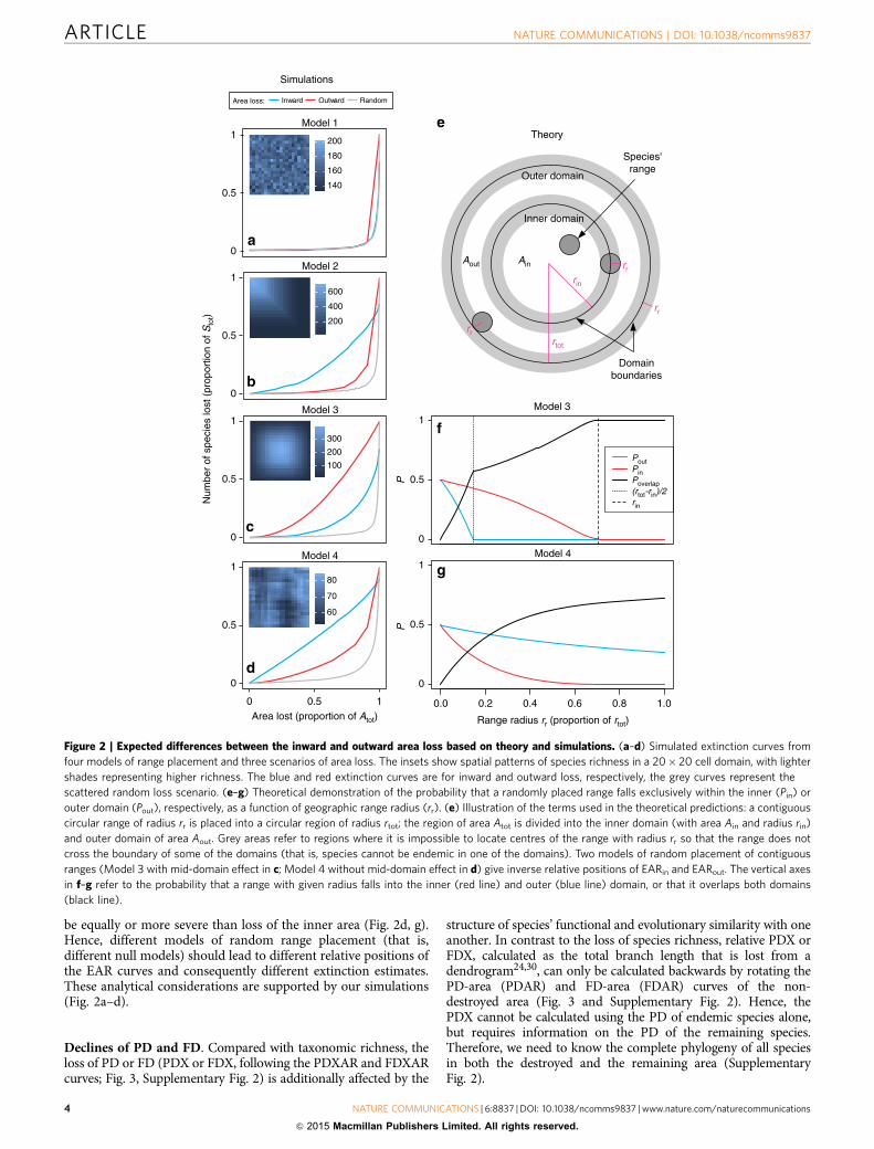
be equally or more severe than loss of the inner area (Fig. 2d, g).Hence, different models of random range placement (that is,different null models) should lead to different relative positions ofthe EAR curves and consequently different extinction estimates.These analytical considerations are supported by our simulations(Fig. 2a–d).

Declines of PD and FD. Compared with taxonomic richness, theloss of PD or FD (PDX or FDX, following the PDXAR and FDXARcurves; Fig. 3, Supplementary Fig. 2) is additionally affected by the

structure of species’ functional and evolutionary similarity with oneanother. In contrast to the loss of species richness, relative PDX orFDX, calculated as the total branch length that is lost from adendrogram24,30, can only be calculated backwards by rotating thePD-area (PDAR) and FD-area (FDAR) curves of the non-destroyed area (Fig. 3 and Supplementary Fig. 2). Hence, thePDX cannot be calculated using the PD of endemic species alone,but requires information on the PD of the remaining species.Therefore, we need to know the complete phylogeny of all speciesin both the destroyed and the remaining area (SupplementaryFig. 2).

Model 3

100

200

300

Model 4

0 0.5 1

60

70

80

Model 2

200

400

600

0

0.5

1

0

0.5

1

0

0.5

1

0

0.5

1

Model 1

140

160

180

200

Num

ber

of s

peci

es lo

st (

prop

ortio

n of

Sto

t)

Area lost (proportion of Atot)

Inward Outward RandomArea loss:

Simulations

Theory

rtot

Aout

rin

Ain

rin

rr

rr

Inner domain

Outer domain

Domainboundaries

rr

Species'range

0.0 0.2 0.4 0.6 0.8 1.0

Model 3

0

0.5

1

0

0.5

1

PP

Range radius rr (proportion of rtot)

Model 4

PoutPinPoverlap(rtot-rin)/2rin

Figure 2 | Expected differences between the inward and outward area loss based on theory and simulations. (a–d) Simulated extinction curves from

four models of range placement and three scenarios of area loss. The insets show spatial patterns of species richness in a 20� 20 cell domain, with lighter

shades representing higher richness. The blue and red extinction curves are for inward and outward loss, respectively, the grey curves represent the

scattered random loss scenario. (e–g) Theoretical demonstration of the probability that a randomly placed range falls exclusively within the inner (Pin) or

outer domain (Pout), respectively, as a function of geographic range radius (rr). (e) Illustration of the terms used in the theoretical predictions: a contiguous

circular range of radius rr is placed into a circular region of radius rtot; the region of area Atot is divided into the inner domain (with area Ain and radius rin)

and outer domain of area Aout. Grey areas refer to regions where it is impossible to locate centres of the range with radius rr so that the range does not

cross the boundary of some of the domains (that is, species cannot be endemic in one of the domains). Two models of random placement of contiguous

ranges (Model 3 with mid-domain effect in c; Model 4 without mid-domain effect in d) give inverse relative positions of EARin and EARout. The vertical axes

in f–g refer to the probability that a range with given radius falls into the inner (red line) and outer (blue line) domain, or that it overlaps both domains

(black line).





Lost species richness (E) is equivalent to PDX or FDX when allspecies are phylogenetically or functionally equivalent, that is,when the dendrogram representing their similarities is rake-shaped (Fig. 3a, green), and only such tree results in aproportional loss of PD (PDX) that is equal to that of E, thatis, the PDXAR and EAR curves are identical. We predict that if atree has ‘tippy’ topology (Fig. 3a, orange), then a species that israndomly selected for extinction will, on average, represent lowerproportion of the total branch lengths of the tree, compared withan extinction that occurs in a tree that has ‘stemmy’ or rake-liketopology (Fig. 3a, green). As a consequence, the initial loss of PDshould be less pronounced than the loss of species richness, andthe PDXAR curves should be below the EAR curves (Fig. 3b). Inother words, any redundancy among species’ functional orphylogenetic information, that is, increasing deviation from arake-shape topology, will result in an initial loss of PD that is lesspronounced than the loss of species richness. The same principlesapply for the loss of FD (FDX) or other dendrogram-basedmetrics.

Empirical extinction curves at large scales. We find that foramphibians, birds and mammals in nine regions on four con-tinents, simulated inward area loss leads to greater loss of speciesrichness than outward area loss, and that the randomly scatteredhabitat loss leads to lowest loss of richness (Fig. 4). The pro-portion of species predicted to go extinct in a given area is gen-erally highest for amphibians, which corresponds with thisgroup’s generally steeper SARs and EARs26. This is due to therelatively smaller ranges and higher endemicity of amphibians,which results in a predicted species loss that is almostproportional to the inward area loss. As expected, the initialloss of the PD and FD metrics PDX and FDX is always lower thanthe corresponding loss of species richness E (Fig. 5) for all taxa.This difference is particularly pronounced in mammals(Supplementary Fig. 3). In contrast, PD loss is relatively high inamphibians and also in birds in selected African and Asianregions (Supplementary Fig. 3).

Predictors of regional extinction vulnerability. We use areaunder the extinction curve (AUC) as our measure of extinctionvulnerability of a region, with steep curves, that is, high extinctionvulnerability of a region, characterized by high AUC. The mostimportant predictors of AUC were the Inward/Outward/Random

geometry of the habitat loss (averaged (avg.) b of 0, � 1.4 and� 1.8, respectively; Supplementary Table 2) followed by the typeof diversity considered (E or PDX; avg. b¼ � 0.4; SupplementaryTable 2), and three variables describing range geometry. Apartfrom the high extinction vulnerability for inward destruction andfor species richness as a measure of diversity, we also found highvulnerability in taxa with relatively small mean range sizes (avg.b¼ � 0.18), and with autocorrelated (avg. b¼ � 0.26) and morecompact (that is, relatively short perimeter; avg. b¼ � 0.123)species’ geographic ranges (Fig. 6a). In contrast, lower extinctionvulnerability emerges for outward and randomly scattereddestruction, for PD, and in regions and taxa with large, elongatedand/or scattered ranges (Fig. 6a). This confirms our expectationsabout the role of range size26 and shape. Notably, the geometry ofarea loss (inward versus outward or randomly scattered) had astronger effect than all other considered factors (Fig. 6a),including mean geographic range size.

Predictors of discrepancy between inward and outward loss.Two predictors of the EARout-EARin discrepancy (measured asDAUC) had particularly high absolute values of averaged betacoefficients and occurred in the two best models (SupplementaryTable 3): the mean Moran’s I of the ranges (avg. b¼ � 0.43) andthe mean range size (avg. b¼ � 0.32). Specifically, the dis-crepancy was higher in regions and groups with smaller and lessautocorrelated ranges. These two predictors were strongly colli-near (Pearson’s r¼ 0.7, Supplementary Table 1) and hence wewere unable to discriminate between them. Because of its slightlyhigher absolute value of b we report the mean Moran’s I inFig. 6b, but we stress that mean range size may play similarlyimportant role as the autocorrelation of the ranges.

Predictors of discrepancy between EAR and PDXAR. The mostimportant predictors of the discrepancy (DAUC) between the lossof species richness (EAR) and loss of PD (PDXAR) were thefactor describing the geometry of habitat loss (inward, outward orrandom with averaged b of 0, � 1.53 and � 1.66 respectively;Supplementary Table 4) and the Gamma statistic characterizingthe tree (avg. b¼ 0.35; Supplementary Table 4): phylogenetictrees characterized by higher concentration of branching eventstowards the tips (higher Gamma) lose their PD at a relativelyslower rate. We report the model that contains these two pre-dictors in Fig. 6c. Tree ‘stemminess’ emerges as additional

PDtot=Stot

PDtot<Stot

0 Atot

PDtot

PDXAR

PDXAR = EAR

PD

X(p

ropo

rtio

n of

PD

tot)

Proportion of Atot

Atot

Stot

PDtot

Num

ber

of s

peci

es(p

ropo

rtio

n of

Sto

t)

PD

and

PD

X

Area (proportion of A)tot

PDAR in

PDAR out

EAR in

PDXAR in

EAR out

PDXAR out

0

(Aout,PDXout)

(Ain,PDXin)

Figure 3 | Relationship between EAR curves describing the loss of species (E) and PDXAR curves describing the loss of phylogenetic diversity (PDX)

with area loss. (a) Illustrations of our expectation that two different phylogenetic trees lead to two distinct extinction curves (given the same spatial

pattern of area loss) are shown. (b) The PDXAR versus EAR discrepancy in the context of the inward versus outward area loss, using empirical curves for

South-American birds (region SA2) as an example. Note that the PDXAR and PDAR (that is, PD-area) curves follow the same point reflection symmetry as

EAR and SAR, but the PD for the lost area cannot be used for the calculation of PD loss.





relevant predictor (avg. b¼ 0.21; Supplementary Table 4), sug-gesting that the effect of tree topology on the EAR-PDXAR dis-crepancy is better captured by several tree summary statistics,rather than by the Gamma alone.

DiscussionAs inward versus outward extinction curves correspond toSAR-based (backward) versus EAR-based extinction estimates,our results falsify the statement by He and Hubbell12 that‘Species–area relationships always overestimate extinction ratesfrom habitat loss’. More precisely, our models show that the SAR-based backward method (equivalent to inward habitat loss14) cangive higher estimates of diversity loss than the direct EAR-basedmethod, but it can also give lower estimates, depending on thespecific arrangement of species ranges in the region. Thisambiguity emerges at large scales where species distributionsare better described by contiguous blocks rather than by sets ofindividuals (as in ref. 12). The issue arises even under simple nullexpectations of random distribution of ranges, and it criticallydepends on whether the realized (observed) species distributionsemerge as a result of truncation of potential distributions byphysical barriers29 or whether some variant of mid-domainprocess generates the distributions31; our findings bring this long-standing debate from basic macroecology into the context ofapplied extinction science.

Our key empirical finding is that, at large geographic scales, theinward loss of habitats leads to more pronounced declines ofspecies richness than when area is lost from within towards theedges. Our models indicate that this can happen for at least tworeasons: (i) ranges may be non-randomly concentrated close tothe edges for ecological reasons, for example, because of thepresence of suitable habitats in those areas. (ii) Alternatively, thehigher relative impact of inward area loss is expected in randomlydistributed contiguous ranges, when the ranges are truncated or‘cropped’ by region boundary, and this truncation can happen fornatural reasons, for example, coast truncating potential ranges ofa terrestrial species29 (Supplementary Fig. 5b), but it can also bean artefact of the study design, for example, when the focal regionis part of a larger region (Supplementary Fig. 5c), so that rangesalong the edge of the focal region are only parts of larger ranges,overlapping the region boundary. This can easily happen whenEAR curves are constructed for small-scale plots (as in ref. 12)that are arbitrarily delineated within a substantially larger region.


Spe

cies

ric

hnes

s lo

st(p

ropo

rtio

n of

Sto

t)

NA1 SA1 SA2 AF1 AF2 AF3 AS1 AS2 AS3

0

1

0

1

0

1

Bird

sM

amm

als

Am

phib

ians

0 1 0 1 0 1 0 1 0 1 0 1 0 1 0 1 0 1

Inward Outward Random

Figure 4 | Loss of species richness (E) resulting from simulated area loss using empirical species distributions in nine regions and three taxa. Inward

area loss (blue) always leads to higher proportional species loss than outward loss (red), and randomly scattered area loss (grey lines) consistently causes the

lowest proportional loss. The curves are averages of multiple realizations of the habitat destruction in each of the nine regions and in each of the three vertebrate

taxa (birds, mammals, amphibians). The maps at the top row show positions of the nine sampling regions. The shading in the maps indicates altitude.


0

1

0

1

0

1

Bird

sM

amm

als

Am

phib

ians

0 1 0 1 0 1


Div

ersi

ty lo

st (

prop

ortio

n of

tota

l)

FDX

EPDX

Figure 5 | Loss of species richness (E) compared with the decrease of

dendrogram-based measures of diversity (PDX and FDX) due to the

simulated loss of habitable area in nine regions and three taxa. Thin

transparent lines are realizations of the simulations in the nine regions,

thick lines are their averages. Supplementary Fig. 3 provides detailed

comparisons of the curves. Note that compared with mammals and birds

the amphibian phylogeny has a weaker topological resolution and is based

on a number of additional assumptions; see ref. 55 for details. We did not

include the E versus FDX comparison for amphibians here as available data

impeded comparability.





In such a case, the discrepancy between the effect of inward andoutward area loss is not particularly relevant for global speciesextinction, as the species that go extinct within the delineated areaare mostly those that persist outside of it.

Exact quantification of the role of (i) and (ii) is beyond ourscope here. Instead, we provide an inductive statistical model that

predicts the shape of extinctions curves and their discrepancies byfactors that are known to reflect scaling patterns of diversity32.We find that the inward–outward discrepancy is highest whenranges are small and have low spatial autocorrelation (contiguity),but these two aspects are correlated and difficult to separate.Intriguingly, the geometry of area loss (inward versus outward

Par

tial r

esid

uals

for

AU

C

−0.10

0.00

0.10

0.20

−0.10

0.00

0.10

0.20

−0.10

0.00

0.10

0.20

−0.10

0.00

0.10

0.20

−0.10

0.00

0.10

0.20

E PDX

0.17 0.19 0.21

Par

tial r

esid

uals

for

AU

C

0.45 0.55 0.65

Mean 1st class Moran’s IMean of sqrt (range size)/perimeter

0

AUC

1

1Area lost(proportion of Atot)

Lost

div

ersi

ty(p

ropo

rtio

n of

tota

l)

�= –0.39

�= 0.12 �= –0.25

20 40 60 80 100 140

Mean range size (# cells)

�= –0.19


�= –1.4

�= –1.82

AmphibiansMammalsBirds

0.45 0.55 0.65

0.10

0.15

0.20

0.25

0.30

�A

UC

−0.05

0.00

0.05

0.10

−2 0 2 4 6

−0.05

0.00

0.05

0.10

Gamma statistic


Par

tial r

esid

uals

for �

AU

C

0 1

1

Δ AUC

0 1

1

Δ AUC

Area lost(proportion of Atot)

Area lost(proportion of Atot)

Spe

cies

ric

hnes

s lo

st(p

ropo

rtio

n of

Sto

t)D

iver

sity

lost

(pro

port

ion

of to

tal)

EARin

EARout

EAR

PDXAR

Mean 1st class Moran's I ofthe ranges

AmphibiansMammalsBirds

�= –0.43

�= –1.53

�= –1.66

�= 0.28

Figure 6 | Statistical models explaining steepness of regional extinction curves and the discrepancy between different types of curves.

(a) Predictors of regional extinction vulnerability as quantified by the AUC value, (b) the discrepancy (DAUC) between the inward and outward loss of

habitat area and (c) the discrepancy between extinction curves for species richness (EAR) and phylogenetic diversity (PDXAR). Only the single best model,

respectively, is shown (based on lowest AICc score), which includes different predictors in each of the three approaches (see Supplementary Tables 2–4 for

details). Betas (b) are standardized coefficients. We do not provide P-values or standard errors because of a presumed but unknown degree of pseudo-

replication (the same taxon over multiple regions, and vice versa). The Gamma statistic represents ‘stemminess’ of a phylogenetic tree61. Each point stands

for one taxon in one of the nine regions, and/or one measure of diversity where appropriate.





direction of loss) had a substantially stronger effect on thesteepness of the extinction curves than mean geographic rangesize. Given the broadly recognized role of range size for extinctionrisk33,34, these findings are remarkable and point to the need tojointly account for both the range size and the spatial pattern ofthe lost habitable area.

Although the inward versus outward dichotomy representsuseful extremes, real-world habitat destruction rarely happens insuch a defined and contiguous form. Instead, often both inwardhabitat loss (for example, from larger-scale agricultural develop-ment or sea-level rise35–37) and outward area loss from localizedcentres (for example, sprawling cities or large-scale miningoperations) may occur simultaneously. An extreme case of suchsimultaneous loss is captured by our random fragmentationscenario in which the SAR- and EAR- based extinction curves areequivalent. For this scenario, the magnitude of extinctions isalways lower than in the contiguous scenarios (as also reported byrefs 20,21,38), revealing the seriousness of the threat fromincreasing contiguous habitat transformations, as opposed to themore scattered alterations. Note, however, that this applies onlyto immediate biodiversity loss. The scattered area or habitat lossmay actually lead to range fragmentation, which makes speciesmore vulnerable to extinction in the future16,17. More realisticmodels that account for various biological phenomena such ascoexistence mechanisms16, extinction debt21,39,40 or minimumarea requirement41 could help narrow the often broad bounds onexpected biodiversity loss provided by our extreme and simplifiedscenarios. We also see a promising new avenue in the emergingconcept of countryside SAR39, which realistically assumes that thenew habitats replacing the original area are still to some degreehabitable. Unfortunately, some of the more realistic and complexmodels require relatively detailed and context-specificinformation16 and will thus be less generally applicable than themore tractable scenarios presented here.

Some specific demonstrations of how PD can scale with area(PDAR) are now available42,43. However, as we show, such PDARcurves provide no information about the sensitivity of PD to arealoss in the focal region. Addressing this sensitivity requires: (i) theknowledge of the PDAR outside of the focal area and (ii) the pointreflection symmetry of the PDAR and PDXAR curves. These arefundamental issues that require consideration in assessments andpolicy addressing PD decline under area loss. As predicted (andpreviously qualitatively argued for PDAR curves42), thediscrepancy between the loss of species richness (described byEAR) and loss of PD (described by PDXAR) is determined by theshape of the underlying phylogenetic tree: the loss of PD (andother dendrogram-based metrics such as FD) is less pronouncedwhen the extinct species have close relatives or functionallysimilar species in the region, that is, in a ‘stemmy’ rather than‘tippy’ tree shape. For instance, although a single sunbird speciesis lost as habitable area disappears, other members of the cladewould retain a diminishing core of the group’s evolutionary andfunctional attributes, such as mixed nectar and insect feeding,until the extinction of the clade’s final species.

We find that for terrestrial vertebrate groups and their analysedfunctional traits, FD suffers a generally less steep proportionalloss than PD, highlighting that FD may often, and at leastinitially, be more readily retained compared with PD. However,unlike PDXAR, the specifics of the FDXAR curve and thegenerality of this finding will depend on the traits assessed44, theirnumber and respective weighting, and the clustering algorithm(or FD metric), all of which can influence the topology of thefunctional dendrogram45,46. Here, the key insight pertains toqualitative comparison, that is, we can confidently claim that theinitial loss of FD (and other dendrogram-based metrics) willalways be less pronounced than the loss of species richness.

Although the theory on spatial scaling of biodiversity has seenconsiderable progress26,47–49, the scale-dependence ofbiodiversity loss is a complex and yet underdeveloped field, andfurther analyses into the associations that we uncovered areneeded. In line with others20,21,38, we have shown that estimatesof diversity loss based solely on area lost, and ignoring spatialshape (arrangement, direction) of the loss, can be misleading. Thegeometry of area loss is crucial, and must be accounted forwhenever dealing with extinction predictions or managementdecisions. Although habitat transformation of small scatteredareas within a region may be relatively benign until habitatfragmentation leads to large-scale disappearance of whole speciesranges, the destruction of large contiguous blocks of habitatwithin a region may be fatal. Similarly, estimates of counts ofspecies are agnostic to species’ phylogenetic or functionaldistinctness or redundancy. Phylogenetic data, together with atleast basic geographic distribution characteristics and additionaltrait information, is rapidly growing and should increasinglyallow similar evaluations to ours for other clades and regions andenable a more inclusive conservation science that goes beyondvertebrates. As we demonstrate, such information can boundbiodiversity loss expectations and can provide important baselineestimates of the multi-facetted ecological consequences ofongoing and future habitat loss.

MethodsModels of range placement. Here we describe four contrasting models of rangeplacement that were used for our theoretical arguments (Fig. 2). The simulatedrealizations of Models 1–4 (Fig. 2a–d) use rectangular ranges placed on a rectan-gular grid, which is computationally convenient. The analytical reasoning based onModels 3 and 4 (Fig. 2e–g) assumes circular ranges placed into a circular region,which is analytically tractable28.

In Model 1, we assume random placement of scattered ranges. This model usesa region consisting of 20� 20 grid cells of the same area, where each grid cell has aprobability Pi of being occupied by an i-th species, and where Pi is constant acrossgrid cells. The presence or absence of i-th species in each cell is then simulated asan outcome of Bernoulli process with probability Pi. This model produces nospatial aggregation of ranges, and is similar to the random model of He andHubbell12. When averaged across many realizations, this model gives identicalEARin and EARout curves12. Note that He and Hubbell12 demonstrate this onlyimplicitly and use different terminology; they also operate at fine scale usingindividuals as smallest spatial units, whereas here we consider rectangular grid.

In Model 2, we assume non-random placement of contiguous ranges. Real-world large-scale distributions are usually to some degree contiguous, and oftenaggregated. Model 2 takes this to the extreme by using only contiguous ranges andplacing all of them into the upper-left corner of region consisting of 20� 20 gridcells. As a consequence, when Ain¼Aout the difference between Ein and Eout willsimply reflect the number of ranges forced to fall completely into Aout. Thismimics, for example, the presence of strong environmental gradients or barriersconstraining (truncating) species distributions, and in such a case, the differencebetween EARin and EARout is trivial.

Models 3 and 4 use random placement of contiguous ranges (SupplementaryFig. 4). Model 3 places each contiguous range entirely and randomly within theregion, causing highest richness in the centre (mid-domain effect). Model 4 alsoplaces ranges randomly, but allows them to overlap domain edges, effectivelyeliminating the mid-domain effect (see ref. 26 for details of this algorithm).

Simulations from models of range placement. The simulations use square rangesplaced on an artificial rectangular grid (region) of 20� 20 grid cells (Fig. 2a–d; seerefs 16,26 for similar approach). In each simulation run, we place 711 ranges withsizes drawn from empirical range-size frequency distribution observed in the speciesof birds that inhabit 2,200� 2,200 km2 placed in Western Africa (region AF1 inFig. 4). In each run, we calculate mean extinction curves of the inward and outwardscenario (EARin and EARout), as well as scattered random destruction scenarios inwhich grid cells are lost stepwise, one by one, and with the same probability at eachstep. Each simulation run was repeated 100 times, and the resulting 100 extinctioncurves were averaged to produce Fig. 2a–d. The same algorithm was applied toproduce the empirical extinction curves (see below).

Vertebrate distributional data. We used expert-drawn range maps for terrestrialamphibians, birds and mammals in all analyses. The range-maps were based on theIUCN assessment (http://www.iucnredlist.org/) for mammals50 and amphibians51.Distributions for birds were compiled from the best available sources for a given




http://www.iucnredlist.org/


geographical region or taxonomic group1. See also ref. 52 for more details on thedata.

Grid system and study regions. We used an equal area grid originally derived incylindrical equal-area projection withB1� size at the equator and a constant gridcell area Acell of B110� 110 km2. We selected nine square regions (hereafter theregions, Fig. 4 and Supplementary Fig. 1), each of them having a total area (Atot) ofexactly 20� 20 grid cells. The regions were selected so that they lie completelywithin major continental landmasses and each grid cell within the region containsat least some land. The regions were also selected to cover broad variety ofterrestrial biomes, altitudes and latitudes. The nearly identical geometry (note thatregions in higher latitudes are slightly elongated relative to the low latitudes) of theregions enabled us to control for the potentially confounding effects of area andshape, and the extinction curves are thus comparable among the nine regions. Wenote that because of their large size, the study regions are bound to contain distinctenvironmental gradients, and species ranges inside the regions may aggregate alongsuch gradients, similar to the situation in Model 2. This has the potential toenhance the inward–outward discrepancy of the EAR curves.

Extinction curves: species richness (E). We explored three scenarios of habitablearea loss: inward, outward and scattered random. We adopted a strictly nestedsampling design26 to explore the effects of inward and outward scenario (Fig. 1).We considered sampling windows of sides l and area Ain¼Acell� l2, where l 2 Zand 1rlr20. We started with the smallest sampling window (l¼ 1) and with thelargest area outside of the sampling window (Aout¼Atot�Ain). We moved thesampling window continually across the 20� 20 regional grid, and for eachposition, we recorded number of species with ranges exclusively within (Ein) andnumber of species with ranges exclusively outside of (Eout) the sampling window.We calculated mean bEin and bEout by averaging Ein and Eout values across all of thepossible positions of the sampling window. We then enlarged the side of thesampling window to l¼ 2 and we repeated the procedure described above. Wecontinued enlarging the window until l reached 20 and Ain¼Atot, calculating meanbEin and bEout for each of the window areas. We then plotted the proportions bEin=Stot

against Ain/Atot (these are the red EARin curves in Figs 1 and 4 representing theoutward destruction) and bEout=Stotagainst Aout/Atot (these are the blue EARout

curves in Figs 1 and 4 that represent the inward destruction).In the scattered random destruction scenario, we selected the grid cells for the

sampling one by one. The area within the set of selected cells was Ain, and therichness of species endemic to that area was Ein. In each step, each grid cell withinthe remaining area (Atot�Ain) had the same probability of being selected for thedestruction. We repeated this procedure 400 times and averaged the resultingextinction curves to get EARin and EARout.

Extinction curves: PD. We used the most recent and dated phylogenies on thethree vertebrate taxa. For birds, we chose the first tree in the posterior set(distribution) of trees in Jetz et al.53 (see also Jetz et al.23 for discussion of treedating and robustness). We also selected one mammal super-tree from Kuhnet al.54. For amphibians, we used the super-tree from Isaac et al.55. We used theterm PD for the sum of the branch lengths of a phylogenetic tree (or a sub-tree, seebelow)24. In one extreme case (the rake-shaped phylogeny), PD is equivalent tospecies richness (Fig. 3). Let us define several terms (see also Fig. 3 andSupplementary Fig. 2): Let PDtot be the total PD of a region, PDin and PDout arePDs of all of the species occurring inside and outside of the sampling window,respectively, PDEin and PDEout are PDs of species that live exclusively (are endemicto) inside and outside of the window, and PDXin and PDXout are the PD lost due toarea loss. We note that PDXin does not always equal PDEin as we demonstrate inSupplementary Fig. 2b—PDXin is calculated using PDout, whereas calculation ofPDEin does not require PDout. In fact, PDXin¼ PDtot�PDout (SupplementaryFig. 2), and the same principle applies for PDXout. For our purpose, we calculateddPDXin and dPDXout, which is the PDXin and PDXout averaged over all of thepositions of the sampling window of a given area. We plotted the proportionsdPDXin=PDtot against Ain/Atot (the solid PDXARin curve in Fig. 3, representingoutward habitat loss) and dPDXout=PDtotagainst Aout/Atot (the dashed PDXARout

curve in Fig. 3, representing the inward habitat loss).

Extinction curves: FD. We used species-level trait databases of all birds andmammals56 to calculate dendrogram-based FD metric for all grid cellassemblages57. Specifically, we used Gower distance to calculate species pairwisedissimilarity, weighting each of five functional trait categories (diet, body size,activity time and two measures of foraging niche) equally. For detailed descriptionof the traits, see Wilman et al.56, Additional Information and SupplementaryMethods. The species were then clustered by an UPGMA algorithm58 to obtain afunctional dendrogram of each taxon in each region, an approach that insimulation studies has been shown to provide strong representation of originaldissimilarities59. To calculate the proportional loss of FD (FDX), we applied exactlythe same procedure as described above for PD, but using the functionaldendrograms instead of the phylogenetic trees. We did not have a comparablycomprehensive species-level trait database for amphibians, so we did not constructthe FDX curves for this taxon.

Representing regional extinction vulnerability by AUC. We use the AUC (orsimply integral) to represent the abovementioned variation of extinction curves(EAR, PDXAR and FDXAR), with steep curves, that is, high extinction vulner-ability of a region, characterized by high AUC.

Regional predictors. For each of the three major taxa in each of the nine regions,we put together nine predictors (see Supplementary Methods for technical details):(i) Gamma statistic. Tree ‘stemminess’ represented by Pybus and Harvey’s60

gamma statistic (g) characterizes the distribution of branching events within thetree. Trees with go0 have relatively longer inter-nodal distances towards the tips ofthe phylogeny (‘tippy’ trees), whereas trees with g40 have relatively longer inter-nodal distances towards the root of the phylogeny (‘stemmy’ trees). (ii) Stemminess.This is an alternative measure of how ‘tippy’ (or ‘stemmy’) a tree is in a givenregion. It is calculated as Lactual/Lmax, where Lactual is the sum of all branch lengthsin the phylogeny and Lmax is the distance from the tips to the root of the treemultiplied by the total number of tips. (iii) Colless’ index of imbalance61, whichmeasures the branching symmetry of the phylogenetic tree of a given taxon in agiven region. (iv) Mean range size, which is the arithmetic mean (calculated acrossall species) of the total number of grid cells in a given region in which a species was‘detected’ according to the expert-drawn range map. (v) Mean of sqrt(range size)/perimeter. By perimeter we mean the total number of grid-cell sides that form edgesof a gridded area occupied by a species in a given region. We calculated thearithmetic mean of the sqrt(range size)/perimeter over all species of a given taxonthat live in the region. (vi) Mean Moran’s I of the ranges. For each species in eachregion, we measured the autocorrelation of the 1 (occupied) and 0 (unoccupied)values by global Moran’s I58, which is a measure of contiguity of the ranges, and wetook the arithmetic mean (across all species) of the values. (vii) Total richness (orStot) of given taxon in given region. (viii) Richness gradient. We created fine-grain(using 1� cells) map of species richness for each taxon in each region. We thencalculated an ordinary least squares linear regression of the richness in the cellsagainst latitude and longitude of the cells, and their interaction. R2 of thisregression is our index of richness gradient. We interpret it as the magnitude of thelarge-scale spatial autocorrelation of species richness; it also measures howclumped are species ranges towards the edge of the region. (ix) Moran’s I ofrichness, which measured the global first-distance class autocorrelation of cell-specific values of species richness. In contrast to the previous measure, the Moran’sI of richness captures short-distance autocorrelation.

Predictors i–iii capture various aspects of departure of phylogenetic trees fromthe rake-shaped topology, which we hypothesized to be responsible for thePDXAR-EAR discrepancy (Fig. 3 and Supplementary Fig. 2). Predictors iv–videscribe some basic geometrical properties of species geographic ranges in theregions such as range shape, contiguity and complexity of the range edge, whichhave potential links to scaling patterns of biodiversity26,32. Predictor vii representsthe size of the species pool (regional diversity), which was also suggested to affectbeta diversity62 and the associated scaling of species richness. Predictors vii and ixdescribe autocorrelation structure of gradients of species richness, which we expectto broadly correspond with aggregation of species ranges within the domain, asillustrated by our simulations in the inset maps in Fig. 2a–d.

Models explaining AUC and DAUC by the regional predictors. We built threesets of statistical models: (i) Models that explain AUC of all of the EAR andPDXAR curves (162 data points). (ii) Models that explain DAUC of all pairs ofEARin and EARout (27 data points). (iii) Models that explain DAUC of all pairs ofEAR and PDXAR curves (81 data points). By ‘data points’, we mean uniquecombinations of taxa, regions and types of extinction curves. All models used thepredictors described above as predictors and the taxon- and region-specific AUC orDAUC as a response. The specific predictors used in each of the three sets ofmodels are listed in Supplementary Tables 2–4. For all models, we used ordinaryleast squares regression (normal error distribution). We first fitted models with allcombinations of predictors (no interactions or nonlinear terms) and we ranked themodels by their AICc (Akaike Information Criterion with small sample size cor-rection). For all predictors, we also calculated standardized regression coefficients(b) by rescaling each predictor to zero mean and variance of 1, and we averaged thebetas over all of the models (Supplementary Tables 2–4).

All result from modelling, model selection and model averaging aresummarized in Supplementary Tables 2–4. Models presented in Fig. 6 were selectedamong the models given in Supplementary Tables 2–4. When selecting thesemodels we had in mind (i) their interpretability, (ii) out-of-sample predictiveperformance measured by AICc, (iii) number of predictors, (iv) collinearitybetween the predictors (Supplementary Table 1) and (v) how well theycorresponded with the averaged standardized coefficients (b) presented in thesecond line of Supplementary Tables 2–4. Finally, we note that our 27combinations of taxa and regions used for the modelling give a relatively smallsample size and are not independent realizations of a random process. This makesit problematic to calculate likelihoods and limits the interpretation of AICc valuesand model rankings (Supplementary Tables 2–4). Consequently, we do not reportP-values or standard errors.

We note that the standard, published procedures for dendrogram-based FDcalculations are affected by the number, weighting and types of traits assessed44,and the clustering algorithm40,41. These differences may impact the exact





shape of FDXAR curves. We therefore do not analyse these curves or FDXAR andPDXAR differences in detail and instead focus on the qualitative comparisonbetween FDXAR and EAR curves, which is not affected by these methodologicaleffects.

All of the distributional data, phylogenies, functional dendrograms andshapefiles used for the analyses described above are also provided (see AdditionalInformation). Further technical details are in Supplementary Methods.

References1. Jetz, W., Wilcove, D. S. & Dobson, A. P. Projected impacts of climate

and land-use change on the global diversity of birds. PLoS Biol. 5, e157(2007).

2. Butchart, S. H. M. et al. Global biodiversity: indicators of recent declines.Science 328, 1164–1168 (2010).

3. Pereira, H. M. et al. Scenarios for Global Biodiversity in the 21st century.Science 330, 1496–1501 (2010).

4. Jetz, W., McPherson, J. M. & Guralnick, R. P. Integrating biodiversitydistribution knowledge: toward a global map of life. Trends Ecol. Evol. 27,151–159 (2012).

5. Barnosky, A. D. et al. Has the Earth’s sixth mass extinction already arrived?Nature 471, 51–57 (2011).

6. Biton, R. et al. The rediscovered Hula painted frog is a living fossil. Nat.Commun 4, 1959 (2013).

7. Costello, M. J., May, R. M. & Stork, N. E. Can we name Earth’s species beforethey go extinct? Science 339, 413–416 (2013).

8. Pimm, S. L. & Askins, R. A. Forest losses predict bird extinctions in easternNorth America. Proc. Natl. Acad. Sci 92, 9343–9347 (1995).

9. Brook, B. W., Sodhi, N. S. & Ng, P. K. L. Catastrophic extinctions followdeforestation in Singapore. Nature 424, 420–426 (2003).

10. Thomas, C. D. et al. Extinction risk from climate change. Nature 427, 145–148(2004).

11. Malcolm, J. R., Liu, C., Neilson, R. P., Hansen, L. & Hannah, L. Global warmingand extinctions of endemic species from biodiversity hotspots. Conserv. Biol.20, 538–548 (2006).

12. He, F. & Hubbell, S. P. Species-area relationships always overestimateextinction rates from habitat loss. Nature 473, 368–371 (2011).

13. Pan, X. Fundamental equations for species-area theory. Sci. Rep 3, 1334 (2013).14. Pereira, H. M., Borda-de-Agua, L. & Martins, I. S. Geometry and scale in

species-area relationships. Nature 482, E3–E4 (2012).15. He, F. & Hubbell, S. Estimating extinction from species--area relationships: why

the numbers do not add up. Ecology 94, 1905–1912 (2013).16. Matias, M. G. et al. Estimates of species extinctions from species–area

relationships strongly depend on ecological context. Ecography 37, 431–442(2014).

17. Rybicki, J. & Hanski, I. Species–area relationships and extinctions caused byhabitat loss and fragmentation. Ecol. Lett. 16, 27–38 (2013).

18. Kinzig, A. P. & Harte, J. Implications of endemics-area relationship forestimates of species extinctions. Ecology 81, 3305–3311 (2000).

19. Ney-Nifle, M. & Mangel, M. Habitat loss and changes in the species-arearelationship. Conserv. Biol. 14, 893–898 (2000).

20. Ulrich, W. & Buszko, J. Habitat reduction and patterns of species loss. BasicAppl. Ecol. 5, 231–240 (2004).

21. Ramage, B. S., Marshalek, E. C., Kitzes, J. & Potts, M. D. Conserving tropicalbiodiversity via strategic spatiotemporal harvest planning. J. Appl. Ecol. 50,1301–1310 (2013).

22. Pimm, S. L. et al. The biodiversity of species and their rates of extinction,distribution, and protection. Science 344, 1246752 (2014).

23. Jetz, W. et al. Global distribution and conservation of evolutionary distinctnessin birds. Curr. Biol. 24, 919–930 (2014).

24. Faith, D. P. Conservation evaluation and phylogenetic diversity. Biol. Conserv.61, 1–10 (1992).

25. Flynn, D. F. B., Mirotchnick, N., Jain, M., Palmer, M. I. & Naeem, S. Functionaland phylogenetic diversity as predictors of biodiversity–ecosystem-functionrelationships. Ecology 92, 1573–1581 (2011).

26. Storch, D., Keil, P. & Jetz, W. Universal species-area and endemics-arearelationships at continental scales. Nature 488, 78–81 (2012).

27. Axelsen, J. B., Roll, U., Stone, L. & Solow, A. Species–area relationships alwaysoverestimate extinction rates from habitat loss: comment. Ecology 94, 761–763(2013).

28. Allen, A. P. & White, E. P. Effects of range size on species-area relationships.Evol. Ecol. Res 5, 493–499 (2003).

29. Sizling, A. L., Storch, D. & Keil, P. Rapoport’s rule, species tolerances, and thelatitudinal diversity gradient: geometric considerations. Ecology 90, 3575–3586(2009).

30. Cadotte, M. W. Experimental evidence that evolutionarily diverse assemblagesresult in higher productivity. Proc. Natl Acad. Sci. USA 110, 8996–9000 (2013).

31. Grytnes, J. A. Ecological interpretations of the mid-domain effect. Ecol. Lett. 6,883–888 (2003).

32. Storch, D., Marquet, P. A. & Brown, J. H. Scaling Biodiversity (CambridgeUniv., 2007).

33. Lande, R. Risks of population extinction from demographic and environmentalstochasticity and random catastrophes. Am. Nat. 142, 911–927 (1993).

34. Cardillo, M. et al. Multiple causes of high extinction risk in large mammalspecies. Science 309, 1239–1241 (2005).

35. Ferraz, G. et al. Rates of species loss from Amazonian forest fragments. Proc.Natl Acad. Sci. USA 100, 14069–14073 (2003).

36. Laurance, W. F. & Balmford, A. Land use: a global map for road building.Nature 495, 308–309 (2013).

37. Wetzel, F. T., Beissmann, H., Penn, D. J. & Jetz, W. Vulnerability of terrestrialisland vertebrates to projected sea-level rise. Glob. Change Biol. 19, 2058–2070(2013).

38. Kallimanis, A. S., Kunin, W. E., Halley, J. M. & Sgardelis, S. P. Metapopulationextinction risk under spatially autocorrelated disturbance. Conserv. Biol. 19,534–546 (2005).

39. Pereira, H. M. & Daily, G. C. Modelling biodiversity dynamics in countrysidelandscapes. Ecology 87, 1877–1885 (2006).

40. Wearn, O. R., Reuman, D. C. & Ewers, R. M. Extinction debt and windows ofconservation opportunity in the Brazilian Amazon. Science 337, 228–232(2012).

41. Pe’er, G. et al. Toward better application of minimum area requirements inconservation planning. Biol. Conserv. 170, 92–102 (2014).

42. Morlon, H. et al. Spatial patterns of phylogenetic diversity. Ecol. Lett. 14,141–149 (2011).

43. Helmus, M. R. & Ives, A. R. Phylogenetic diversity–area curves. Ecology 93,S31–S43 (2012).

44. Maire, E., Grenouillet, G., Brosse, S. & Villeger, S. How many dimensions areneeded to accurately assess functional diversity? A pragmatic approach forassessing the quality of functional spaces. Glob. Ecol. Biogeogr 24, 728–740(2015).

45. Mouchet, M. et al. Towards a consensus for calculating dendrogram-basedfunctional diversity indices. Oikos 117, 794–800 (2008).

46. Pavoine, S., Vallet, J., Dufour, A.-B., Gachet, S. & Daniel, H. On the challenge oftreating various types of variables: application for improving the measurementof functional diversity. Oikos 118, 391–402 (2009).

47. He, F. & Legendre, P. Species diversity patterns derived from species-areamodels. Ecology 83, 1185–1198 (2002).

48. Harte, J., Smith, A. B. & Storch, D. Biodiversity scales from plots to biomes witha universal species-area curve. Ecol. Lett. 12, 789–797 (2009).

49. Sizling, A. L., Kunin, W. E., Sizlingova, E., Reif, J. & Storch, D. Betweengeometry and biology: the problem of universality of the species-arearelationship. Am. Nat. 178, 602–611 (2011).

50. Schipper, J. et al. The status of the World’s land and marine mammals:diversity, threat, and knowledge. Science 322, 225–230 (2008).

51. Buckley, L. B. & Jetz, W. Linking global turnover of species and environments.Proc. Natl Acad. Sci. USA 105, 17836–17841 (2008).

52. Belmaker, J. & Jetz, W. Cross-scale variation in species richness–environmentassociations. Glob. Ecol. Biogeogr 20, 464–474 (2011).

53. Jetz, W., Thomas, G. H., Joy, J. B., Hartmann, K. & Mooers, A. O.The global diversity of birds in space and time. Nature 491, 444–448(2012).

54. Kuhn, T. S., Mooers, A. Ø. & Thomas, G. H. A simple polytomy resolver fordated phylogenies: Resolving polytomies under a birth-death model. MethodsEcol. Evol 2, 427–436 (2011).

55. Isaac, N. J. B., Redding, D. W., Meredith, H. M. & Safi, K. Phylogenetically-informed priorities for amphibian conservation. PLoS ONE 7, e43912(2012).

56. Wilman, H. J. et al. EltonTraits 1.0: Species-level foraging attributes of theworld’s birds and mammals. Ecology 95, 2027 (2014).

57. Petchey, O. L. & Gaston, K. J. Dendrograms and measuring functional diversity.Oikos 116, 1422–1426 (2007).

58. Legendre, P. & Legendre, L. Numerical Ecology (Elsevier, 2012).59. Merigot, B., Durbec, J.-P. & Gaertner, J.-C. On goodness-of-fit measure for

dendrogram-based analyses. Ecology 91, 1850–1859 (2010).60. Pybus, O. G. & Harvey, P. H. Testing macro-evolutionary models using

incomplete molecular phylogenies. Proc. Biol. Sci 267, 2267–2272 (2000).61. Davies, T. J. & Buckley, L. B. Exploring the phylogenetic history of mammal

species richness. Glob. Ecol. Biogeogr 21, 1096–1105 (2012).62. Kraft, N. J. B. et al. Disentangling the drivers of b diversity along latitudinal and

elevational gradients. Science 333, 1755–1758 (2011).

AcknowledgementsWe thank to Carsten Meyer and Chia-Ying Ko for parts of the list of amphibiansynonyms. Jonathan Belmaker made comments on an early draft and assisted with thefunctional trees. James Rosindell and Mao-Ning Tuanmu provided valuable comments.Ben S. Carlson improved the language. The research has received funding from thePeople Programme (Marie Curie Actions) of the European Unions Seventh Framework





Programme (FP7/2007–2013) under REA grant agreement no 302868. We are alsograteful to support from NSF grants DBI0960550, DEB-1441737, DEB 1026764 andNASA Biodiversity Grant NNX11AP72G to W.J.

Author contributionsP.K., D.S. and W.J. designed the study and wrote the paper. W.J. provided large part ofthe data. P.K. led the writing, formalized the theoretical arguments, processed the dataand did all analyses, simulations and visualizations.

Additional informationComplete R code, distributional data, phylogenies, functional dendrograms andshapefiles used for the analyses and simulations. The data can be downloaded from Figshare:figshare.com/s/a08c417290df11e49da006ec4bbcf141 (doi:10.6084/m9.figshare.1282334). Thedata come with readme.txt file that contains further details and guidelines for loading thedata and reproducing the analyses.

Supplementary Information accompanies this paper at http://www.nature.com/naturecommunications

Competing financial interests: The authors declare no competing financial interests.

Reprints and permission information is available online at http://npg.nature.com/reprintsandpermissions/

How to cite this article: Keil, P. et al. On the decline of biodiversity due to area loss.Nat. Commun. 6:8837 doi: 10.1038/ncomms9837 (2015).

This work is licensed under a Creative Commons Attribution 4.0International License. The images or other third party material in this

article are included in the article’s Creative Commons license, unless indicated otherwisein the credit line; if the material is not included under the Creative Commons license,users will need to obtain permission from the license holder to reproduce the material.To view a copy of this license, visit http://creativecommons.org/licenses/by/4.0/






http://npg.nature.com/reprintsandpermissions/

http://npg.nature.com/reprintsandpermissions/

http://creativecommons.org/licenses/by/4.0/


On the decline of biodiversity due to area lossstorch/publications/Keil_Storch_Jetz...On the decline...

Documents

Transcript of On the decline of biodiversity due to area lossstorch/publications/Keil_Storch_Jetz...On the decline...