On the Crossover of Boundary Currentsin an Idealized Model of the Red Sea

The MIT Faculty has made this article openly available. Please share how this access benefits you. Your story matters.

Citation Zhai, Ping, Larry J. Pratt, and Amy Bower. “On the Crossover ofBoundary Currents in an Idealized Model of the Red Sea.” Journalof Physical Oceanography 45, no. 5 (May 2015): 1410–1425. © 2015American Meteorological Society

As Published http://dx.doi.org/10.1175/jpo-d-14-0192.1

Publisher American Meteorological Society

Version Final published version

Citable link http://hdl.handle.net/1721.1/100414

Terms of Use Article is made available in accordance with the publisher'spolicy and may be subject to US copyright law. Please refer to thepublisher's site for terms of use.

On the Crossover of Boundary Currents in an Idealized Model of the Red Sea

PING ZHAI

MIT–WHOI Joint Program in Physical Oceanography, Woods Hole Oceanographic Institution,

Woods Hole, Massachusetts, and Department of Marine, Earth and Atmospheric Sciences, North

Carolina State University, Raleigh, North Carolina

LARRY J. PRATT AND AMY BOWER

Department of Physical Oceanography, Woods Hole Oceanographic Institution, Woods Hole, Massachusetts

(Manuscript received 15 September 2014, in final form 27 January 2015)

ABSTRACT

The west-to-east crossover of boundary currents has been seen inmean circulation schemes from several past

models of the Red Sea. This study investigates the mechanisms that produce and control the crossover in an

idealized, eddy-resolving numerical model of the Red Sea. The authors also review the observational evidence

and derive an analytical estimate for the crossover latitude. The surface buoyancy loss increases northward

in the idealized model, and the resultant mean circulation consists of an anticyclonic gyre in the south and a

cyclonic gyre in the north. In themidbasin, the northward surface flow crosses from the western boundary to the

eastern boundary. Numerical experiments with different parameters indicate that the crossover latitude of the

boundary currents changes with f0, b, and the meridional gradient of surface buoyancy forcing. In the analytical

estimate, which is based on quasigeostrophic, b-plane dynamics, the crossover is predicted to lie at the latitude

where the net potential vorticity advection (including an eddy component) is zero. Various terms in the po-

tential vorticity budget can be estimated using a buoyancy budget, a thermal wind balance, and a parameter-

ization of baroclinic instability.

1. Introduction

The Red Sea is an example of an ‘‘inverse estuary’’ in

which surface buoyancy loss far exceeds the gain because

of freshwater input. It differs from theMediterranean Sea

and fromother prominentmarginal seas in its narrow and

meridionally elongated geometry. In fact, its latitude

range is such that the Coriolis parameter f doubles from

the south to the north tip, resulting in a novel situation in

which zonal motion is encouraged by a strong beta effect

but suppressed by narrow geometry.

Observations of the Red Sea circulation are tem-

porally and spatially sparse, and many properties of the

climatological circulation are uncertain. Robust features

include the overturning circulation, which occupies the

upper 300m in the north and upper 150m in the south

and whose annual transport of about 0.36 Sverdrups

(Sv; 1 Sv5 106m3 s21) is based on measurements within

the strait of Bab el Mandeb (BAM) (Murray and Johns

1997). There is also striking transition in summer to a

three-layer exchange flow in the BAM, which is thought

to be because of the summer reversal in thewind direction

in the southernRed Sea andGulf ofAden as well as in the

Arabian Sea (Smeed 1997, 2000, 2004; Yao et al. 2014a,b).

Another feature that appears in multiple observations is a

cyclonic gyre, approximately 300m deep, at the northern

end (Vercelli 1927; Morcos 1970; Morcos and Soliman

1974; Maillard 1974; Clifford et al. 1997), believed to

be a site of convection and Red Sea overflow water pro-

duction (Sofianos and Johns 2003). Many inferences

about the general circulation come from numerical sim-

ulations (e.g., Clifford et al. 1997; Eshel and Naik 1997;

Siddall et al. 2002; Sofianos et al. 2002; Sofianos and Johns

2003; Biton et al. 2008, 2010; Chen et al. 2014; Yao et al.

2014a,b), most of which reproduce the northernmost

gyre but which can differ in other aspects. There have

been very few analytical models, laboratory experiments,

Corresponding author address: Ping Zhai, Department ofMarine,

Earth and Atmospheric Sciences, North Carolina State University,

Jordan Hall, RM 4145, Raleigh, NC 27695-8208.

E-mail: pingzhai425@gmail.com

1410 JOURNAL OF PHYS ICAL OCEANOGRAPHY VOLUME 45

DOI: 10.1175/JPO-D-14-0192.1

� 2015 American Meteorological Society

or idealized numerical simulations apart from the cele-

brated Phillips (1966) model, but his restriction to a two-

dimensional overturning cell and his neglect of rotation

are limiting.

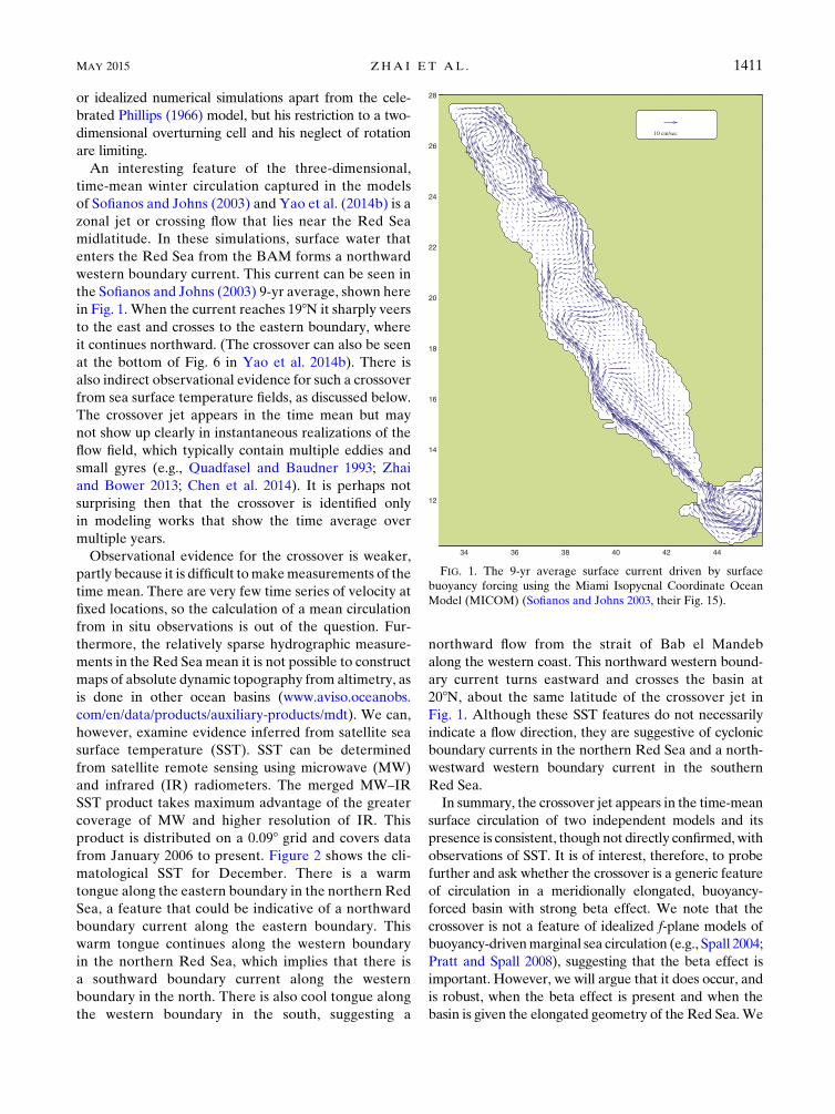
An interesting feature of the three-dimensional,

time-mean winter circulation captured in the models

of Sofianos and Johns (2003) and Yao et al. (2014b) is a

zonal jet or crossing flow that lies near the Red Sea

midlatitude. In these simulations, surface water that

enters the Red Sea from the BAM forms a northward

western boundary current. This current can be seen in

the Sofianos and Johns (2003) 9-yr average, shown here

in Fig. 1. When the current reaches 198N it sharply veers

to the east and crosses to the eastern boundary, where

it continues northward. (The crossover can also be seen

at the bottom of Fig. 6 in Yao et al. 2014b). There is

also indirect observational evidence for such a crossover

from sea surface temperature fields, as discussed below.

The crossover jet appears in the time mean but may

not show up clearly in instantaneous realizations of the

flow field, which typically contain multiple eddies and

small gyres (e.g., Quadfasel and Baudner 1993; Zhai

and Bower 2013; Chen et al. 2014). It is perhaps not

surprising then that the crossover is identified only

in modeling works that show the time average over

multiple years.

Observational evidence for the crossover is weaker,

partly because it is difficult tomakemeasurements of the

time mean. There are very few time series of velocity at

fixed locations, so the calculation of a mean circulation

from in situ observations is out of the question. Fur-

thermore, the relatively sparse hydrographic measure-

ments in the Red Sea mean it is not possible to construct

maps of absolute dynamic topography from altimetry, as

is done in other ocean basins (www.aviso.oceanobs.

com/en/data/products/auxiliary-products/mdt). We can,

however, examine evidence inferred from satellite sea

surface temperature (SST). SST can be determined

from satellite remote sensing using microwave (MW)

and infrared (IR) radiometers. The merged MW–IR

SST product takes maximum advantage of the greater

coverage of MW and higher resolution of IR. This

product is distributed on a 0.098 grid and covers data

from January 2006 to present. Figure 2 shows the cli-

matological SST for December. There is a warm

tongue along the eastern boundary in the northern Red

Sea, a feature that could be indicative of a northward

boundary current along the eastern boundary. This

warm tongue continues along the western boundary

in the northern Red Sea, which implies that there is

a southward boundary current along the western

boundary in the north. There is also cool tongue along

the western boundary in the south, suggesting a

northward flow from the strait of Bab el Mandeb

along the western coast. This northward western bound-

ary current turns eastward and crosses the basin at

208N, about the same latitude of the crossover jet in

Fig. 1. Although these SST features do not necessarily

indicate a flow direction, they are suggestive of cyclonic

boundary currents in the northern Red Sea and a north-

westward western boundary current in the southern

Red Sea.

In summary, the crossover jet appears in the time-mean

surface circulation of two independent models and its

presence is consistent, though not directly confirmed, with

observations of SST. It is of interest, therefore, to probe

further and ask whether the crossover is a generic feature

of circulation in a meridionally elongated, buoyancy-

forced basin with strong beta effect. We note that the

crossover is not a feature of idealized f-plane models of

buoyancy-drivenmarginal sea circulation (e.g., Spall 2004;

Pratt and Spall 2008), suggesting that the beta effect is

important. However, we will argue that it does occur, and

is robust, when the beta effect is present and when the

basin is given the elongated geometry of the Red Sea.We

FIG. 1. The 9-yr average surface current driven by surface

buoyancy forcing using the Miami Isopycnal Coordinate Ocean

Model (MICOM) (Sofianos and Johns 2003, their Fig. 15).

MAY 2015 ZHA I ET AL . 1411

will also show that the crossover depends on the presence

of a northward increase in the surface buoyancy flux,

also a feature of the Red Sea air–sea interaction.Wewill

explore the dynamics of the crossover and present an

analytical estimate of its latitude as a function of f0, b,

and the northward gradient of the surface buoyancy flux.

This work is organized as follows: Section 2 describes the

numerical simulation of the buoyancy-driven circulation

in an idealized Red Sea using an eddy-resolving general

circulation model. Section 3 introduces an ad hoc an-

alytical estimate, centered on the buoyancy equation

and on potential vorticity dynamics, of parameter

dependencies of the crossover latitude. Section 4 offers

some conclusions.

2. Numerical model simulation of the buoyancy-driven circulation in an idealized Red Sea

a. Model description

The Massachusetts Institute of Technology general

circulation model (MITgcm) (Marshall et al. 1997) is

used to simulate the buoyancy-driven circulation in an

idealized Red Sea. The model used in this study is

nonhydrostatic and solves the momentum and density

equations on a Cartesian, staggered Arakawa C grid.

The parameters that are used in the control experiment

(EXPT0) are described in this section, whereas param-

eter settings for other experiments are listed in Table 1.

The model domain includes the idealized Red Sea, the

strait of Bab el Mandeb, and the Gulf of Aden (Fig. 3).

The idealizedRed Sea is a rectangular basin with a width

of 300 km and a length of 1600km. The Gulf of Aden is

600km wide and 250km long. In the Red Sea and the

Gulf of Aden, the bottom depth increases from 0m at

the coast to 1000m over an offshore distance of 80 km.

The strait of Bab el Mandeb is 100km wide and 150 km

long, with a sill depth of 200m. The horizontal grid

spacing is 5 km, and there are 29 vertical levels, with

thickness varying from 10m at the surface to 100m at the

bottom. The Coriolis parameter in EXPT0 is approxi-

mated by f 5 f0 1 by with f0 5 3.5 3 1025 s21 and

b 5 2.1 3 10211m21 s21, which are typical of the Red

Sea. The term f0 is the Coriolis parameter at the south-

ern boundary of the model domain.

The model is forced by surface fluxes of heat Q

and freshwater E in the Red Sea. In EXPT0, Q

changes linearly from 0 at the southern end of the Red

Sea (y 5 400 km) to 220Wm22 at the northern end

FIG. 2. Climatological MW–IR SST (8C) for December.

TABLE 1. Model run parameters and symbols used in Fig. 13. B0 5 ay 1 b represents the surface buoyancy flux, and YC is the crossover

latitude. Units are B0 (kgm22 s21); f0 (s

21); b (m21 s21); a (kgm23 s21); b (kgm22 s21); and crossover YC (km).

EXPT f0 (3 1025) b (3 10211) a (3 10212) b (3 1026) YC Symbol

EXPT0 3.5 2.1 3.5 21.4 1028 DEXPT1 1.5 2.1 3.5 21.4 1351 d

EXPT2 2.5 2.1 3.5 21.4 1139 d

EXPT3 7.0 2.1 3.5 21.4 798 d

EXPT4 10.5 2.1 3.5 21.4 674 d

EXPT5 3.5 0.5 3.5 21.4 852 DEXPT6 3.5 1.5 3.5 21.4 995 DEXPT7 3.5 4 3.5 21.4 1152 DEXPT8 3.5 6 3.5 21.4 1218 DEXPT9 3.5 2.1 0 2.8 658 O

EXPT10 3.5 2.1 1.7 0.7 927 O

EXPT11 3.5 2.1 2.6 20.34 989 O

EXPT12 3.5 2.1 4.3 22.4 1074 O

1412 JOURNAL OF PHYS ICAL OCEANOGRAPHY VOLUME 45

(y 5 2000 km), and E increases linearly from 0 at the

southern end of the Red Sea to 4.3myr21 at the

northern end. We use a linear equation of state, such

that r5 rr(12 aTT1 bSS), where rr5 999.8 kgm23 is a

reference density and aT 5 2 3 1024 8C21 and bS 5 8 31024 are thermal expansion and haline contraction co-

efficients. The surface buoyancy flux (Fig. 3) calculated

from Q and E is B0 52aTQ/cw 1 r0bSS0E, where cw 53900Jkg21 8C21 is the heat capacity of water. In this

model, surface freshwater flux changes the salinity of

seawater but cannot affect the total volume. The buoy-

ancy flux B0 has units of kilograms per square meter per

second and increases linearly with latitude according to

B0 5 ay 1 b (Table 1).

In the numerical experiments shown in Table 1, the

mean buoyancy flux over the whole Red Sea remains

fixed.We will be particularly interested in how themean

circulation is affected by variations in the distribution of

the surface buoyancy flux and in f0 and b. The initial

conditions for temperature and salinity are based on

average profiles of temperature and salinity measured

from theMarch 2010 and September–October 2011 Red

Sea cruises (Bower 2010; Bower and Abualnaja 2011;

Bower and Farrar 2015). The temperature and salinity in

the eastern part of the Gulf of Aden (Fig. 3) are relaxed

to these initial profiles with a relaxation time scale of

60 days.We have tried different relaxation profiles in the

eastern Gulf of Aden and different choices of relaxation

profiles do not influence the circulation pattern. The

relaxation of temperature and salinity in the Gulf of

Aden acts as a source of buoyancy to balance the surface

buoyancy losses in the Red Sea. Second-order viscosity

and diffusivity are used to parameterize subgrid-scale

processes. In the area outside the strait and west from

the buffer zone, the surface buoyancy flux is zero. The

vertical viscosity and diffusivity for temperature and

salinity are 1025m2 s21. The vertical diffusivity is in-

creased to 1000m2 s21 when the water column is hy-

drostatically unstable in order to simulate convection.

There is no explicit horizontal diffusivity of temperature

and salinity in the model. The Smagorinsky viscosity nSis used to determine the horizontal viscosity, such that

Ah 5 (vS/p)2L2

ffiffiffiffiffiffiffiffiffiffiffiffiffiffiffiffiffiffiffiffiffiffiffiffiffiffiffiffiffiffiffiffiffiffiffiffiffiffiffiffiffiffiffiffiffiffi(ux 2 yy)

2 1 (uy 1 yx)2

q, where L is the

spacing scale, u and y are horizontal velocities, and

subscripts represent partial derivatives. Recommended

values for nS are in the range of 2.2 to 4 for large-scale

oceanic simulations (Griffies and Hallberg 2000); we

have chosen nS 5 2.5. No slip boundary conditions are

applied at bottom and lateral boundaries.

Themodel is run for 25 yr with steady surface heat loss

and evaporation and reaches a quasi-steady state. Un-

less it is explicitly stated otherwise, the mean fields dis-

cussed in this study will be the average over the final 5 yr

of the 25-yr simulation.

b. Numerical model results

The benchmark experiment EXPT0 reveals a set of

gyres and boundary currents that establish pathways for

the northward movement of lighter water from the strait

through the Red Sea basin. As indicated in Fig. 4, which

shows a 5-yr mean surface velocity and density, the sur-

face inflow from the Gulf of Aden brings lighter water

into the Red Sea through the strait of Bab el Mandeb.

When the inflow enters the Red Sea, it turns left and

continues moving northward along the western boundary

until it reaches about 1000km, where it turns east and

crosses the basin. Because of the surface buoyancy losses,

the density of each boundary current increases as the

inflow moves northward. To the north of the crossover

FIG. 3. Model domain with bottom topography (colors, m) and

EXPT0 surface buoyancy loss (white contours with contour interval

of 0.5 3 1026 kgm22 s21 and with zero contour at Y 5 400 km).

Temperature and salinity in the region east of the dashed white line

are restored to the initial profiles.

MAY 2015 ZHA I ET AL . 1413

latitude, the surface boundary circulation is cyclonic; in

the southern Red Sea, it is predominantly anticyclonic.

Two snapshots of the surface temperature (Fig. 4)

from EXPT0 suggest the same general configuration of

boundary currents and crossover as in the 5-yr mean

fields. Eddies are also present in the snapshots, and the

crossover in one snapshot occurs slightly to the south of

its mean position near 1000km, while the crossover in

another snapshot occurs to the north of its mean posi-

tion. The eddies may be instrumental in transporting

warm and freshwater from the boundary currents to the

interior where heat and freshwater are lost because of

surface cooling and evaporation, as described by Spall’s

2004 f-plane experiment.

The zonal sections of meridional velocity at y 5 500

and 1770km are plotted in Fig. 5. The vertical structure

of the meridional velocity at y 5 1770km indicates that

the cyclonic boundary circulation in the northern Red

Sea is intensified in the upper 200m with maximum

speed in excess of 30 cm s21. Recall that 200m is also the

sill depth for the southern strait. Below 200m, there is a

much weaker anticyclonic circulation with speed less

than 5 cm s21. The zonal section of meridional velocity

at y 5 500km indicates that the circulation in the

southern Red Sea is also intensified in the upper 200m.

The western boundary current can extend to 800m.

However its speed below 200m is very weak. The

weaker, northward-flowing eastern boundary current

only penetrates down to 100m and overlies a counter-

current that extends from 100 to 300m and is situated

slightly offshore. The maximum velocity of the surface

northward flow is about 5 cm s21 and that of the sub-

surface southward countercurrent is about 10 cm s21.

The countercurrent returns water in the Red Sea

back to the strait. Therefore, the vertical, integrated

boundary current on the eastern boundary is southward

and the depth-integrated circulation in the southern

Red Sea is predominantly anticyclonic. Overall, the

surface circulation associated with waters entering

the model domain through the strait is stronger than

the intermediate circulation that carries the return

flow. The primary reason for this mismatch is the pres-

ence of a strong recirculation component in the surface

flow, especially in the northern basin.

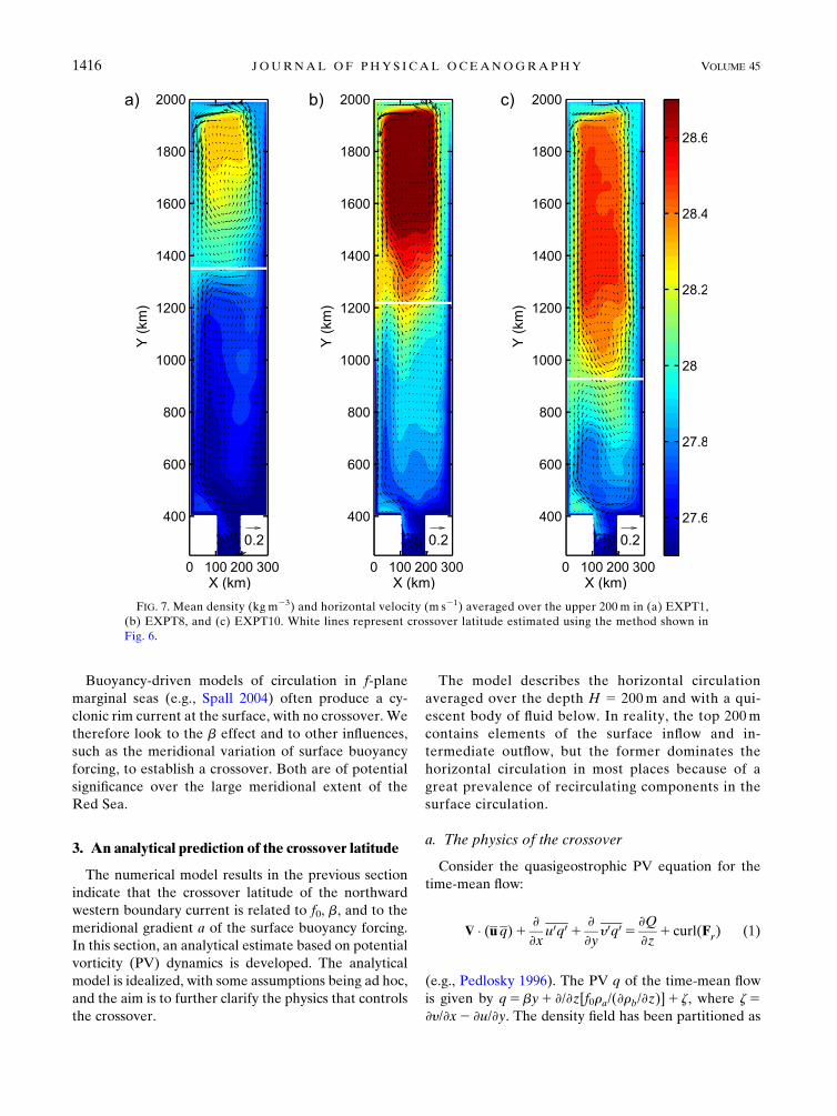
The determination of the crossover latitude of the

northward western boundary current in the numerical

model is illustrated in Fig. 6. The crossover latitude is

defined as the zero-crossing point of themeanmeridional

velocity on the western boundary, taken as the average

meridional velocity within 80km of the western coast and

FIG. 4. (a) Mean density (kgm23) and horizontal velocity (m s21) for EXPT0 averaged over the upper 200m.

(b),(c) Two snapshots of the surface temperature from EXPT0 (contour interval is 0.38C).

1414 JOURNAL OF PHYS ICAL OCEANOGRAPHY VOLUME 45

in the upper 200m. (In our model, 80km is the offshore

topographic width scale and also the approximate width

of the boundary current.) In EXPT0, the crossover lati-

tude of the western boundary is 1028km. Subsequent

numerical experiments with different parameters will

indicate that the crossover latitude varies with f0, b, and

the meridional gradient of surface buoyancy fluxes. As

shown in Table 1 and Fig. 7, the crossover latitude moves

to 1351km when f0 5 1.5 3 1025 s21 (EXPT1) or to

1218km when b is increased to 6 3 10211m21 s21

(EXPT8). In EXPT10, the meridional gradient of surface

buoyancy flux is reduced, and the crossover latitude shifts

to 927km.

Sofianos and Johns (2003) suggested that crossover

occurs at the latitude above which Rossby waves with the

frequency of the forcing (2p yr21 in their study) are no

longer possible and only Kelvin waves exist. Their argu-

ment is based on a study of eastern boundary currents by

McCreary et al. (1986, hereinafter MSK86), in which a

subtropical ocean is subject to time-periodic, wind, and

buoyancy forcing at frequencys. The critical latitude for a

long Rossby wave with this frequency, and with vertical

mode number n, is shown to be ucr 5 tan21[cn/(2Rs)],

where R is Earth’s radius. Poleward of ucr, this wave

becomes Kelvin-like, decaying away from the eastern

boundary over the Rossby radius of deformation. The

argument then is that western boundary layer dynamics

should prevail at the annual frequency south of ucr, while

an eastern boundary layer should exist to the north.

Sofianos and Johns (2003) find reasonable agreement

between their observed crossover latitude and the value

of ucr obtained by choosing s as the seasonal frequency

(2p yr21) and by choosing the second baroclinic mode

(n 5 2) and computing the associated vertical eigen-

value cn. One difficulty with this approach is that

the crossover exists in our model (and in that of Yao

et al. 2014b) in the presence of steady forcing. For this

case, s 5 0, and the above prediction would put the

crossover at 908N. In addition, the crossover latitude in

the mean field does not change significantly if an an-

nual cycle is substituted for the steady forcing, as il-

lustrated in Fig. 8 for the EXPT0 simulation with and

without an annual cycle. It was mentioned in the in-

troduction that the crossover is identified only in a time

average over multiple years. Because of the presence of

eddies in the instantaneous field, it is difficult to esti-

mate crossover latitude for time periods shorter than a

few months. There are some other interesting com-

parisons with theMSK86, and these will be discussed in

the final section.

FIG. 5. Zonal sections ofmeanmeridional velocity (contour interval is 5 cm s21) fromEXPT0 at

(a) y 5 500 km and (b) y 5 1770 km. Zero velocity contour is plotted in thick black lines.

FIG. 6. Mean western boundary current speed, which is calcu-

lated as the average meridional velocity in the western boundary

(within 80 km of the western boundary) in the upper 200m. The

crossover latitude YC is defined as the zero-crossing point.

MAY 2015 ZHA I ET AL . 1415

Buoyancy-driven models of circulation in f-plane

marginal seas (e.g., Spall 2004) often produce a cy-

clonic rim current at the surface, with no crossover. We

therefore look to the b effect and to other influences,

such as the meridional variation of surface buoyancy

forcing, to establish a crossover. Both are of potential

significance over the large meridional extent of the

Red Sea.

3. An analytical prediction of the crossover latitude

The numerical model results in the previous section

indicate that the crossover latitude of the northward

western boundary current is related to f0, b, and to the

meridional gradient a of the surface buoyancy forcing.

In this section, an analytical estimate based on potential

vorticity (PV) dynamics is developed. The analytical

model is idealized, with some assumptions being ad hoc,

and the aim is to further clarify the physics that controls

the crossover.

The model describes the horizontal circulation

averaged over the depth H 5 200m and with a qui-

escent body of fluid below. In reality, the top 200m

contains elements of the surface inflow and in-

termediate outflow, but the former dominates the

horizontal circulation in most places because of a

great prevalence of recirculating components in the

surface circulation.

a. The physics of the crossover

Consider the quasigeostrophic PV equation for the

time-mean flow:

$ � (u q)1 ›

›xu0q0 1

›

›yy0q05

›Q

›z1 curl(Fr) (1)

(e.g., Pedlosky 1996). The PV q of the time-mean flow

is given by q5by1 ›/›z[f0ra/(›rb/›z)]1 z, where z5›y/›x2 ›u/›y. The density field has been partitioned as

FIG. 7. Mean density (kg m23) and horizontal velocity (m s21) averaged over the upper 200 m in (a) EXPT1,

(b) EXPT8, and (c) EXPT10. White lines represent crossover latitude estimated using the method shown in

Fig. 6.

1416 JOURNAL OF PHYS ICAL OCEANOGRAPHY VOLUME 45

r(x, y, z)5 rb(z)1 ra(x, y, z), and Q and Fr represent

unspecified heating and friction functions. The overbar

represents a time average, and primes are deviations

from the time average.

Now integrate (1) over a volume extending throughout

the active layers and enclosed by a rectangular circuit C

that contains a segment of the western boundary current

and extends slightly offshore of its outer edge (Fig. 9):

ðL0

ðy2

y1

ð02H

0@›y q

›y1

›y0q0

›y1

›u0q0

›x

1Adz dy dx5

ððA

C

Qz50 dA1

þC

ð02H

Fr � dz dl .

The left integrand contains the divergence of mean and

eddy PV fluxes, and these could be integrated and

written as a sum of fluxes across the lateral boundaries of

the box. The net flux of PV out of the box by the mean

flow and by the eddies must be balanced by generation

of PV inside the box by heating/cooling at the surface

and by frictional stresses acting tangentially alongC. We

will assume that the meridional flux of PV is primarily

due to the mean flow and therefore that the second inte-

grand on the left-hand side is neglected. We will further

assume that the main contribution to the frictional term

comes from the solid boundary. Also, if the boundary

current is narrow and the surface buoyancy loss is spread

evenly across the width of the basin, then the thermal

forcing term is likely negligible compared to offshore eddy

flux since the latter must supply the buoyancy that is lost

in the interior. With these assumptions, the PV budget is

ðL0

ðy2

y1

ð02H

0@›y q

›y1

›u0q0

›x

1A dy dz dx5

þC

ð02H

Fr � dz dl .

(2)

Although we have not specified the form of the fric-

tional vector Fr, we will assume that it opposes the flow

FIG. 8. Mean surface density (kgm23) and horizontal velocity (m s21) in (a) EXPT0 with steady forcing and (b) an

experiment using surface buoyancy forcing with annual cycle. The surface buoyancy forcing used in (b) has a form of

ay1 b1 c cos(t). (c) The values in January (maximum) and July (minimum) are plotted. The annual-mean buoyancy

forcing indicated by the thick black line is the same as EXPT0.

MAY 2015 ZHA I ET AL . 1417

along the wall. For a western boundary current as shown

in Fig. 9, we anticipate the main frictional contribution

will come from the segment of C corresponding to the

wall so thatÞC

Ð 02H Fr � dz dl52

Ð y2y1

Ð 02H F(y)

r jx5L dz dy.

A northward boundary current will be associated

with a negative Fr(y), and (2) then indicates that the

divergence of the potential vorticity flux (integrand

on the left) must be positive. This is the situation that

would exist for the northward flow of a linear, baro-

tropic western boundary layer on a beta plane (q5 by)

and with no eddies. If the same situation were postu-

lated on the eastern boundary, the sign of the friction

term would reverse but the divergence of the eddy flux

would remain the same, so (2) would no longer hold.

This reasoning would then constitute an argument for

western intensification.

If q is dominated by the stretching term, with

stratification weakening toward the north, so that

›/›z[f0ra/(›rb/›z)] decreases in the northward direc-

tion, then the signs in the eddy-free version of (2) are

self-consistent only if the friction comes from the

eastern segment of the integration contour C. The

geographic eastern boundary becomes the ‘‘dynamical’’

western boundary. In the Red Sea, where thermal

convection in the north is expected to weaken strati-

fication, it is possible that q will be dominated by by in

the south, and by the stretching term in the north, with

dq/dy vanishing at some intermediate latitude. In an

eddy-free environment, this would be the crossover

latitude.However, the real situation is complicated by the

presence of the eddy term in (2), and the general condi-

tion that must be satisfied at the crossover latitude is that

the total advection (mean plus eddy) of PV is zero. This

is the physical basis for the estimation of the crossover

latitude, though further analysis and assumptions are

required to write the fluxes in terms of the governing

parameters of the model.

b. Assumptions

Figure 10 shows the assumed flow configuration and

geometrical parameters used to produce the estimate of

the crossover latitude YC. This picture is based on a

number of assumptions:

1) The surface water that enters the Red Sea through

the BAM moves northward along the western Red

Sea boundary (current I) and crosses over to the

FIG. 10. A schematic diagram illustrating the boundary currents in

the ad hoc analytical model.

FIG. 9. A schematic diagram showing the structure of the

boundary current.

1418 JOURNAL OF PHYS ICAL OCEANOGRAPHY VOLUME 45

eastern boundary at latitude YC. (That the current

should begin on the west coast is in agreement with

the numerical model runs for nonzero b. In the actual

Red Sea, the value of b is largest in the south, and the

surface buoyancy forcing is weakest there. It stands

to reason that the northward potential vorticity

gradient will be dominated by b in the south, leading

to westward intensification there.) To the north, the

circulation is dominated by a set of cyclonic bound-

ary currents (III, IV, and V).

2) The horizontal velocity components vary weakly

with z over 0$ z$2H but rapidly go to zero below

the base of this layer (z 5 2H).

3) The boundary layer dynamics are linear, meaning

that contribution to q from relative vorticity z is

weaker than the planetary contribution by or that

from the stretching term. This assumption is not

always met in the numerical simulations, but it is

invoked here to enable closure.

4) The surface buoyancy loss to the atmosphere in the

interiors of the gyres is balanced by eddy buoyancy

fluxes from boundary currents III, IV, and V into the

interior. The importance of such eddy fluxes has been

emphasized in a number of observations and model

results from other marginal seas (e.g., Visbeck et al.

1996; Marshall and Schott 1999; Spall 2004, 2011,

2013; Pratt and Spall 2008; Isachsen and Nost 2012).

We further assume that the eddy buoyancy flux is

proportional to the mean boundary current velocity

VbN of boundary currents III, IV, and V (Stone 1972;

Visbeck et al. 1996; Spall and Chapman 1998; Spall

2004) and to the density difference between the

boundary current and the interior. For the eddy

fluxes from boundary currents III, IV, and V into

the interior of the northern gyres, this parameteriza-

tion takes the form

u0r05 cVbN(rinN 2 rbN) , (3)

where c is a nondimensional coefficient represent-

ing the efficiency of buoyancy transport by the

baroclinic eddy (c is related to the ratio of bottom

slope to isopycnal slope; Spall 2004); rbN is mean

density of boundary currents III, IV, and V, aver-

aged over its length, width, and depth; and rinN is the

density of the interior region in the northern gyre,

assumed to be constant. With this formulation the

eddy buoyancy flux is constant along the length of

the boundary layer.

5) VbN is in thermal wind balance:

VbN 5Hg

2r0 fC

rinN 2 rbNL

, (4)

where L is the width of boundary current and is

approximated using the width of bottom slope (80km).

The equation fC 5 f0 1bYC defines the Coriolis pa-

rameter at the southern boundary of the northern gyre.

Since the analytical model is applied in the northern

gyre, fC is used as a reference Coriolis parameter in (4)

and the following calculations.

6) The wind stress is ignored, though we will later

speculate on its effect.

7) The density varies linearly with depth over the

surface layer of thickness H and has constant value

r0 below. Specifically,

r(x, y, z)5

([12N2(z1H)/g]r01 2hrai(z1H)/H, z$2H

r0, z,2H.

Thus, the background stratification rb(z) 5[12N2(z1H)/g]r0 (also the stratification of the

resting state) has constant value N in the surface

layer. The perturbation density ra 5 2hrai(z1H)/H

also varies linearly with z, and its vertical average

hrai over the surface layer is a function of x and y.

(The assumption of linearly varying density in the

surface layer is in rough agreement with the nu-

merical simulations, as suggested in Fig. 11.)

This concludes the list of assumptions. The goal now is

to evaluate the terms in the left-hand side of (2), with the

integration box located at the eastern boundary (as de-

picted by the blue rectangle in Fig. 10). We begin

calculating the mean advection of PV. Its vertical aver-

age hy qi over the surface layer is

hy qi5 y

H

ð02H

by2

fCg

r0

›

›z

raN2

!dz

5 y

by2

fCg

r0H

rajz502 rajz52H

N2

!.

The density perturbation in the deep region is zero

(rajz52H5 0), and thus rajz50

5 2hrai, so that

hy qi5 yby22fCg

r0

hraiHN2

y . (5)

MAY 2015 ZHA I ET AL . 1419

Similarly, the eddy flux of potential vorticity is

hu0q0i522fCg

r0HN2u0hr0ai . (6)

Angle brackets are dropped in the following calcula-

tion for convenience.

The divergence of the northward advection of density

within an eastern boundary current is balanced by sur-

face buoyancy loss to the atmosphere over the boundary

current and zonal eddy fluxes of buoyancy from the

boundary current into the interior, thus the buoyancy

budget for boundary current III can be written as

›

›y

ðXE

XE2L

y ra dx2 u0r0ajx5X

E2L

5LB0(y)

H. (7)

Here, u0r0a is the zonal eddy buoyancy flux. A more

detailed derivation of (7) appears in appendix A.

With the help of (5) and (6), the left-hand side of (2)

can now be written as

ðXE

XE2L

ðy2

y1

0@›y q

›y1

›u0q0

›x

1A dy dx5

ðXE

XE2L

ðy2

y1

24›yby

›y2

2fCg

r0HN2

0@›y ra

›y1

›u0r0a›x

1A35 dy dx

5

ðy2

y1

26664›

›y

ðXE

XE2L

yby dx22fCg

r0HN2

›

›y

ðXE

XE2L

y ra dx2 u0r0ajx5XE2L

!375dy . (8)

If (7) is used to simplify the final expression in paren-

theses, and the result is substituted into (2), it follows

that

L

ðy2

y1

›yby

›y2

2fCgB0

r0H2N2

!dy5

ððAcurlFr dx dy .

The integrand on the left-hand side represents the

divergence of the advection of PV within the box. It in-

cludes contributions from mean and eddy fluxes. The

predicted YC lies where the integrand vanishes, that is,

›yby

›y2

2fCgB0(y)

r0H2N2

5 0 (at y5YC) , (9)

where B0 5 ay 1 b.

To compute YC from (9), one needs to estimate the

velocity y in terms of known parameters. This involves a

series of algebraic steps that use the parameterization of

baroclinic instability [(3)], the thermal wind condition

[(4)], and the buoyancy budget for the northern gyre

as a whole. The resulting septic equation for YC along

with a prediction of the density difference between the

boundary current and the interior are developed in

appendix B [see (B3) and (B4)].

c. PV constraints on the boundary currents andcrossover latitude

The predicted value of the crossover latitude YC is

shown in Fig. 12 as a function of f0, b, and themeridional

FIG. 11. (a) A schematic diagram of density profile in the analytical model. (b) Density

profiles in EXPT0. The thick black line represents mean density profile, and thin black lines

represent density profiles at different locations.

1420 JOURNAL OF PHYS ICAL OCEANOGRAPHY VOLUME 45

gradient a of the surface buoyancy flux. In computingYC

in the analytical model we have chosen N2 as 2.2 31025 s22, which is an average value in the model domain

in EXPT0. The empirical constant c ranges from 0.008 to

0.03 through estimations in numerical experiments by

using (3), and c5 0.015 is used in the analytical estimate.

Sensitivity of the predicted YC to N2 and c will be

discussed below.

According to (9), the planetary PV advection is

proportional to b, while the magnitude of the buoyancy

loss term increases with f0 and surface buoyancy loss.

As a result, the crossover latitude is anticipated to in-

crease with b and decrease with f0, which is supported

by Fig. 12. Equation (9) also suggests that the buoyancy

loss term increases with the meridional gradient a of

the surface buoyancy flux (as contained in the param-

eter B0 5 ay 1 b), and Fig. 12 confirms that when

a decreases, the predicted and actual crossover latitude

moves farther south. Essentially, a decrease in a causes

the surface buoyancy losses to become stronger in the

southernRed Sea and the contribution of stretching PV

increases. Comparisons between the analytical pre-

diction and numerical model for all model runs are

shown in Fig. 13. The prediction tends to overestimate

YC when YC is large and underestimate YC when YC is

small. There is also a strong linear relationship between

the predicted and numerical model values. The two

agree with a least squares fit slope of 0.78 and a cor-

relation coefficient of 0.97.

The comparisons of rinN 2 rbN and VbN are shown in

Fig. 13. They also reveal good agreement between the

numerical model and the ad hoc analytical model. The

predicted and numerical model results of rinN 2 rbN are

linearly related with a correlation of 0.91 and a least

squares fit slope of 1.06. According to (B3), rinN 2 rbNincreases with f0 and b. The value rinN 2 rbN also in-

creases with the meridional gradient a of the surface

buoyancy flux. This is because when a increases, the

surface buoyancy losses become stronger in the north-

ern Red Sea. Thus, a larger rinN 2 rbN is required to

generate larger eddy buoyancy fluxes to balance surface

buoyancy losses in the interior region. The predicted

and numerical model results of VbN are linearly related

FIG. 12. Variations of crossover latitude due to variations

in (a) f0, (b) b, and (c) the meridional gradient of surface

buoyancy loss a. The parameters for each experiment are given

in Table 1.

FIG. 13. Comparison of (a) crossover latitude, (b) density difference, and (c) boundary velocity between the analytical prediction and

a series of numericalmodel results. Themeaning of different types of symbols is described in Table 1. Black dots correspond to changing f0,

red triangles correspond to variable b, and blue circles correspond to the variable meridional gradient (a) of surface buoyancy flux. The

black line is the least squares fit line to the points plotted in this figure.

MAY 2015 ZHA I ET AL . 1421

with a correlation of 0.95 and a least squares fit slope of

1.01. The term VbN also increases with a, which can be

explained by thermal wind relation [(4)]. Equation (4)

also indicates that VbN decreases with f0 and b.

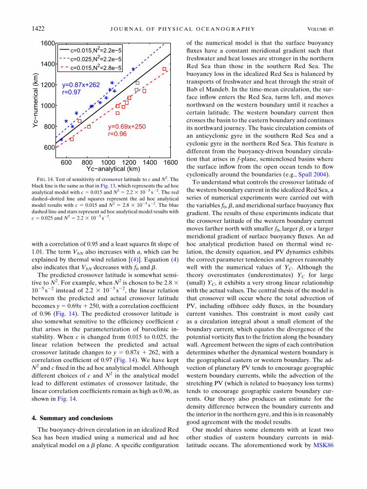
The predicted crossover latitude is somewhat sensi-

tive to N2. For example, when N2 is chosen to be 2.8 31025 s22 instead of 2.2 3 1025 s22, the linear relation

between the predicted and actual crossover latitude

becomes y5 0.69x1 250, with a correlation coefficient

of 0.96 (Fig. 14). The predicted crossover latitude is

also somewhat sensitive to the efficiency coefficient c

that arises in the parameterization of baroclinic in-

stability. When c is changed from 0.015 to 0.025, the

linear relation between the predicted and actual

crossover latitude changes to y 5 0.87x 1 262, with a

correlation coefficient of 0.97 (Fig. 14). We have kept

N2 and c fixed in the ad hoc analytical model. Although

different choices of c and N2 in the analytical model

lead to different estimates of crossover latitude, the

linear correlation coefficients remain as high as 0.96, as

shown in Fig. 14.

4. Summary and conclusions

The buoyancy-driven circulation in an idealized Red

Sea has been studied using a numerical and ad hoc

analytical model on a b plane. A specific configuration

of the numerical model is that the surface buoyancy

fluxes have a constant meridional gradient such that

freshwater and heat losses are stronger in the northern

Red Sea than those in the southern Red Sea. The

buoyancy loss in the idealized Red Sea is balanced by

transports of freshwater and heat through the strait of

Bab el Mandeb. In the time-mean circulation, the sur-

face inflow enters the Red Sea, turns left, and moves

northward on the western boundary until it reaches a

certain latitude. The western boundary current then

crosses the basin to the eastern boundary and continues

its northward journey. The basic circulation consists of

an anticyclonic gyre in the southern Red Sea and a

cyclonic gyre in the northern Red Sea. This feature is

different from the buoyancy-driven boundary circula-

tion that arises in f-plane, semienclosed basins where

the surface inflow from the open ocean tends to flow

cyclonically around the boundaries (e.g., Spall 2004).

To understand what controls the crossover latitude of

the western boundary current in the idealizedRed Sea, a

series of numerical experiments were carried out with

the variables f0, b, and meridional surface buoyancy flux

gradient. The results of these experiments indicate that

the crossover latitude of the western boundary current

moves farther north with smaller f0, larger b, or a larger

meridional gradient of surface buoyancy fluxes. An ad

hoc analytical prediction based on thermal wind re-

lation, the density equation, and PV dynamics exhibits

the correct parameter tendencies and agrees reasonably

well with the numerical values of YC. Although the

theory overestimates (underestimates) YC for large

(small) YC, it exhibits a very strong linear relationship

with the actual values. The central thesis of the model is

that crossover will occur where the total advection of

PV, including offshore eddy fluxes, in the boundary

current vanishes. This constraint is most easily cast

as a circulation integral about a small element of the

boundary current, which equates the divergence of the

potential vorticity flux to the friction along the boundary

wall. Agreement between the signs of each contribution

determines whether the dynamical western boundary is

the geographical eastern or western boundary. The ad-

vection of planetary PV tends to encourage geographic

western boundary currents, while the advection of the

stretching PV (which is related to buoyancy loss terms)

tends to encourage geographic eastern boundary cur-

rents. Our theory also produces an estimate for the

density difference between the boundary currents and

the interior in the northern gyre, and this is in reasonably

good agreement with the model results.

Our model shares some elements with at least two

other studies of eastern boundary currents in mid-

latitude oceans. The aforementioned work by MSK86

FIG. 14. Test of sensitivity of crossover latitude to c and N2. The

black line is the same as that in Fig. 13, which represents the ad hoc

analytical model with c 5 0.015 and N2 5 2.2 3 1025 s22. The red

dashed–dotted line and squares represent the ad hoc analytical

model results with c 5 0.015 and N2 5 2.8 3 1025 s22. The blue

dashed line and stars represent ad hoc analytical model results with

c 5 0.025 and N2 5 2.2 3 1025 s22.

1422 JOURNAL OF PHYS ICAL OCEANOGRAPHY VOLUME 45

centers on a semi-infinite ocean with an eastern

boundary and with buoyancy and wind forcing. The

buoyancy forcing increases to the north, producing a sea

surface that slopes down toward the north and a geo-

strophically balanced flow toward the east. This flow is

brought to zero at the eastern boundary by a boundary

layer that relies on thermal diffusion to achieve a vor-

ticity balance. The boundary current has poleward sur-

face flow, with surface sinking, and there is weaker,

equatorward undercurrent. The model results include

cases of steady forcing along with cases of seasonal

forcing, but the domain of interest lies to the south of the

critical latitudes for the first two baroclinic, Rossby wave

modes in all cases. Although there is no western

boundary and nothing like a crossover jet, the structure

of the eastern boundary current may share some ele-

ments with that in our model, which also has poleward

surface flowwith an opposing undercurrent. (This aspect

is lost in the averaging that we do over the upper 200m

of our model but is worthy of further investigation.)

Pedlosky and Spall (2005, hereinafter PS05) analyze a

buoyancy-forced, two-layer circulation in a rectangular

domain. The PS05 model involves steady, b-plane flow,

so the whole domain essentially lies to the south of the

relevant Rossby wave critical latitude. The buoyancy

forcing, which is introduced as a cross-interface velocity,

increases linearly to the north and produces the same

eastward geostrophic flow as in MSK86. The model also

admits an eastern thermal ‘‘boundary layer,’’ in which

sinking takes place, but in the asymptotic setting ex-

plored by PS05, this layer covers the interior. The linear,

quasigeostrophic analytical model has a southward

western boundary current at all latitudes within the

domain, with smooth, eastward flow in the interior not

crossover jet. Primitive equation numerical simulations

are also presented, and one of these produces a closed,

cyclonic gyre in the north, similar to that seen in our

simulations (e.g., Fig. 4). But again, there is no distinct

crossover jet. The discrepancy between PS05 and this

study might be because of the model configuration. The

inflow transport in their analytical model is weak by

assumption and is specified, while the inflow transport in

our study is part of the solution. The buoyancy forcing in

our model is imposed as a surface buoyancy flux,

whereas their forcing is imposed by restoring an in-

terface to some predetermined shape. Thus, the result-

ing spatial pattern of forcing is different. In addition, the

sloping boundary in our model may have a substantial

influence on the physics of the boundary layers.

Buoyancy-driven circulation in the idealized Red Sea

consists of an anticyclonic boundary circulation in the

southern Red Sea and a cyclonic boundary circulation in

the northern Red Sea. This circulation pattern is similar

in some respects to that of the subtropical and subpolar

gyres of the North Atlantic and North Pacific. However,

it is generally agreed that these gyres are driven by wind,

whereas the Red Sea circulation is primarily determined

by buoyancy forcing (Sofianos and Johns 2003).

The crossover latitude moves southward in the nu-

merical experiment with surface wind stress in Sofianos

and Johns (2003). Further to the issue of wind forcing, it

is natural to ask how wind might influence the crossover

latitude. The simplest way of introducing a wind stress

would be to incorporate it as a body force t/rH, evenly

distributed over the depth of the upper 200m. The

function (2) then becomes

ðL0

ðy2

y1

ð02H

24›y q

›y1›u0q0

›x2 curl

�t

rH

�35dy dz dx5

þC

ð02H

Fr � dz dl .

The crossover occurs where the friction term on the right

vanishes, as before. If the wind stress curl is negative, the

corresponding term agrees in sign with the term in-

volving b (hidden in y q), and this would tend to move

the crossover latitude northward, provided that the eddy

flux term remains the same. The wind stress curl in

winter in the southern Red Sea in Sofianos and Johns

(2003) is positive. Thus, the crossover latitude moves

southward in their study.

Although our formal prediction of the crossover lat-

itude differs from what Sofianos and Johns (2003) sug-

gest, with ours based on a steady state and theirs based

on seasonal time dependence, the underlying mechanisms

share some common elements. Both involve potential

vorticity dynamics, and both contemplate a basin in

which the beta effect, westward propagation of Rossby

waves, and westward intensification dominate in the

southern portion. In Sofianos and Johns (2003),

b decreases in the northward direction, and there

exists a latitude beyond which propagation of long

Rossby waves at the annual frequency is not supported.

In our scenario, the beta effect is reversed at higher

latitude by vortex stretching due to diverging iso-

pycnals and possibly by offshore eddy fluxes of poten-

tial vorticity. In our study, both the ad hoc analytical

model and numerical model suggest that it is the

MAY 2015 ZHA I ET AL . 1423

competition between the advection of planetary vor-

ticity and the buoyancy loss term in the PV budget that

determines the crossover latitude.

Acknowledgments. We have benefited from talking

with Tom Farrar, Jiayan Yang, Paola Rizzoli, and Mike

Spall. This work is supported by Award USA 00002,

KSA 00011, and KSA 00011/02 made by King Abdullah

University of Science and Technology (KAUST), by

National Science Foundation Grants OCE0927017,

OCE1154641, andOCE85464100, and by theWoodsHole

Oceanographic Institution Academic Program Office.

APPENDIX A

Simplification of the Density Equation

The density equation can be written as

›u ra›x

1›y ra›y

1›w ra›z

1›u0r0a›x

1›y0r0a›y

1›w0r0a›z

5B0

H.

We now integrate this equation vertically over the

thickness H of the upper layer and also from the outer

edge x5XE 2 L of the eastern boundary current to the

position x5XE of the eastern wall. We will assume that

the vertical velocity vanishes or is negligibly small at z5 0

and also at z 5 2H (consistent with the assumption

that H is constant). We also set u 5 u0 5 0 at the wall,

and we further assume that the northward advection of

density by the time-averaged flow is much larger than

the northward eddy flux of density y ra � y0r0a. This allleads to (7).

APPENDIX B

Development of the Relationship for the CriticalLatitude YC

To derive the prediction for YC, we begin by ap-

proximating the velocity in (9) with the average velocity

VbN in boundary currents III, IV, and V. Use of the

thermal wind relation [(4)] for VbN then leads to

bN2H2

4f 2C(rinN 2 rbN)5

LB0(YC)

H, (B1)

where B0(YC)5 aYC 1 b. To get an expression for

(rinN 2 rbN), we consider the buoyancy budget for the

northern gyre as a whole. As suggested in Fig. 10, the sea

surface buoyancy loss in the interior region (shaded in

blue in Fig. 10) in the northern gyre is assumed to be

balanced by lateral eddy fluxes originating from

boundary currents III, IV, and V. Thus, the buoyancy

budget can be written as

[2LinN(YC)1WinN]Hu0r0 5ðA

N

B0 dA5WinNBTN(YC) ,

(B2)

where LinN(YC)5YN 2 (3L/2)2YC and WinN are the

length and width of the interior region in the northern

gyre; AN 5LinNWinN is the area of interior region; H is

the vertical scale of the boundary current; and

BTN(YC)5

ðYN2L

YC1L/2

B0 dy .

If (B2) is combined with the thermal wind relation [(4)]

for VbN and with the parameterization of baroclinic in-

stability [(3)], one obtains an expression for the density

difference between the boundary current and the

interior:

rinN 2 rbN 5

ffiffiffiffiffiffiffiffiffiffiffiffiffiffiffiffiffiffiffiffiffiffiffiffiffiffiffiffiffiffiffiffiffiffiffiffiffiffiffiffiffiffiffiffi2r0 fCLWinNBTN

cH2g(2LinN 1WinN)

s. (B3)

Substitution for the density difference in (B1) leads to

bN2H2

4fC(YC)2

ffiffiffiffiffiffiffiffiffiffiffiffiffiffiffiffiffiffiffiffiffiffiffiffiffiffiffiffiffiffiffiffiffiffiffiffiffiffiffiffiffiffiffiffiffiffiffiffiffiffiffiffiffiffiffiffi2r0 fC(YC)LWinNBTN(YC)

cg[2LinN(YC)1WinN]

s5LB0(YC) .

(B4)

Given that B0 and LinN are linear in YC, and that BTN is

quadratic inYC, it follows that (B4) is essentially a septic

equation for YC, though in practice it is solved in the

above form.

REFERENCES

Biton, E., H. Gildor, and W. R. Peltier, 2008: Red Sea during the

Last Glacial Maximum: Implications for sea level re-

construction. Paleoceanography, 23, PA1214, doi:10.1029/

2007PA001431.

——, ——, G. Trommer, M. Siccha, M. Kucera, M. T. J. van der

Meer, and S. Schouten, 2010: Sensitivity of Red Sea circulation

to monsoonal variability during the Holocene: An integrated

data and modeling study. Paleoceanography, 25, PA4209,

doi:10.1029/2009PA001876.

Bower, A., 2010: Cruise report—R/V Aegaeo KAUST leg1

northeastern Red Sea, 16-29March 2010. WHOI Tech. Rep.

WHOI-KAUST-CTR-2010-01, 28 pp.

——, and Y. Abualnaja, 2011: Cruise report—R/V Aegaeo

KAUST leg1 eastern Red Sea, 15 September-10 October

2011. WHOI Tech. Rep. WHOI-KAUST-CTR-2011-01,

25 pp.

——, and J. Farrar, 2015: Air-sea interaction and horizontal

circulation in the Red Sea. The Red Sea: The Formation,

1424 JOURNAL OF PHYS ICAL OCEANOGRAPHY VOLUME 45

Morphology, and Environment of a Young Ocean Basin,

N. Rasul and I. Stuart, Eds., Springer, 329–342.

Chen, C., and Coauthors, 2014: Process modeling studies of phys-

ical mechanisms of the formation of an anticyclonic eddy in

the central Red Sea. J. Geophys. Res. Oceans, 119, 1445–1464,

doi:10.1002/2013JC009351.

Clifford, M., C. Horton, J. Schmitz, and L. H. Kantha, 1997: An

oceanographic nowcast/forecast system for the Red Sea.

J. Geophys. Res., 102, 25 101–25 122, doi:10.1029/97JC01919.

Eshel, G., andN.H.Naik, 1997: Climatological coastal jet collision,

intermediate water formation, and the general circulation of

the Red Sea. J. Phys. Oceanogr., 27, 1233–1257, doi:10.1175/1520-0485(1997)027,1233:CCJCIW.2.0.CO;2.

Griffies, S. M., and R. W. Hallberg, 2000: Biharmonic friction

with a Smagorinsky-like viscosity for use in large-scale eddy-

permitting ocean models. Mon. Wea. Rev., 128, 2935–2946,

doi:10.1175/1520-0493(2000)128,2935:BFWASL.2.0.CO;2.

Isachsen, P. E., and O. A. Nost, 2012: The air sea transformation

and residual overturning circulation within the Nordic Seas.

J. Mar. Res., 70, 31–68, doi:10.1357/002224012800502372.

Maillard, C., 1974: Eaux intermediaires et formation d’eau pro-

fonde en Mer Rouge. L’Oceanographie Physique de la Mer

Rouge, CNEXO, 105–133.

Marshall, J., and F. Schott, 1999: Open-ocean convection: Observa-

tions, theory, and models. Rev. Geophys., 37, 1–64, doi:10.1029/

98RG02739.

——, C. Hill, L. Perelman, and A. Adcroft, 1997: Hydrostatic,

quasi-hydrostatic, and nonhydrostatic ocean modeling.

J. Geophys. Res., 102, 5733–5752, doi:10.1029/96JC02776.

McCreary, J. P., S. R. Shetye, and P. K. Kundu, 1986: Thermoha-

line forcing of eastern boundary currents: With application to

the circulation off the west coast of Australia. J. Mar. Res., 44,

71–92, doi:10.1357/002224086788460184.

Morcos, S., 1970: Physical and chemical oceanography of the Red

Sea. Oceanogr. Mar. Biol., 8, 73–202.

——, and G. F. Soliman, 1974: Circulation and deep water for-

mation in the northern Red Sea in winter. L’Oceanographic

Physique de la Mer Rouge, CNEXO, 91–103.

Murray, S. P., and W. Johns, 1997: Direct observations of seasonal

exchange through the Bab el Mandeb strait. Geophys. Res.

Lett., 24, 2557–2560, doi:10.1029/97GL02741.

Pedlosky, J., 1996:OceanCirculation Theory. Springer-Verlag, 453 pp.

——, and M. A. Spall, 2005: Boundary intensification of vertical

velocity in a b-plane basin. J. Phys. Oceanogr., 35, 2487–2500,

doi:10.1175/JPO2832.1.

Phillips, O. M., 1966: On turbulent convection currents and the

circulation of the Red Sea. Deep-Sea Res. Oceanogr. Abstr.,

13, 1149–1160.

Pratt, L. J., andM. Spall, 2008: Circulation and exchange in choked

marginal seas. J. Phys. Oceanogr., 38, 2639–2661, doi:10.1175/

2008JPO3946.1.

Quadfasel, D., and H. Baudner, 1993: Gyre-scale circulation cells

in the Red-Sea. Oceanol. Acta, 16 (3), 221–229.

Siddall, M., D. A. Smeed, S. Matthiesen, and E. J. Rohling, 2002:

Modelling the seasonal cycle of the exchange flow in Bab El

Mandab (Red Sea). Deep-Sea Res. I, 49, 1551–1569,

doi:10.1016/S0967-0637(02)00043-2.

Smeed, D. A., 1997: Seasonal variation of the flow in the strait of

Bab al Mandab. Oceanol. Acta, 20 (6), 773–781.

——, 2000: Hydraulic control of three-layer exchange flows: Appli-

cation to the Bab al Mandab. J. Phys. Oceanogr., 30, 2574–2588,doi:10.1175/1520-0485(2000)030,2574:HCOTLE.2.0.CO;2.

——, 2004: Exchange through the Bab al Mandab. Deep-Sea Res.

II, 51, 455–474, doi:10.1016/j.dsr2.2003.11.002.

Sofianos, S. S., and W. E. Johns, 2003: An Oceanic General Cir-

culation Model (OGCM) investigation of the Red Sea circu-

lation: 2. Three-dimensional circulation in the Red Sea.

J. Geophys. Res., 108, 3066, doi:10.1029/2001JC001185.——,——, and S. P. Murray, 2002: Heat and freshwater budgets in

theRed Sea fromdirect observations at Bab elMandeb.Deep-

Sea Res., 49, 1323–1340.

Spall, M. A., 2004: Boundary currents and water mass trans-

formation in marginal seas. J. Phys. Oceanogr., 34, 1197–1213,

doi:10.1175/1520-0485(2004)034,1197:BCAWTI.2.0.CO;2.

——, 2011: On the role of eddies and surface forcing in the heat

transport and overturning circulation in marginal sea.

J. Climate, 24, 4844–4858, doi:10.1175/2011JCLI4130.1.

——, 2013: On the circulation of Atlantic Water in the Arctic

Ocean. J. Phys. Oceanogr., 43, 2352–2371, doi:10.1175/

JPO-D-13-079.1.

——, and D. C. Chapman, 1998: On the efficiency of baroclinic

eddy heat transport across narrow fronts. J. Phys. Ocean-

ogr., 28, 2275–2287, doi:10.1175/1520-0485(1998)028,2275:

OTEOBE.2.0.CO;2.

Stone, P., 1972: A simplified radiative–dynamical model for the static

stability of rotating atmospheres. J. Atmos. Sci., 29, 405–418,

doi:10.1175/1520-0469(1972)029,0405:ASRDMF.2.0.CO;2.

Vercelli, E., 1927: Richerche di oceanografia fisica eseguite della

R. N. AMMIRAGLIO MAGNAGHI (1923– 24), 4, la tem-

peratura e la salinita. Ann. Idrogr., 11, 1–66.Visbeck, M., J. Marshall, and H. Jones, 1996: Dynamics of iso-

lated convective regions in the ocean. J. Phys. Oceanogr.,

26, 1721–1734, doi:10.1175/1520-0485(1996)026,1721:

DOICRI.2.0.CO;2.

Yao, F., I. Hoteit, L. J. Pratt, A. S. Bower, P. Zhai, A. Köhl, andG. Gopalakrishnan, 2014a: Seasonal overturning circula-

tion in the Red Sea: 1. Model validation and summer cir-

culation. J. Geophys. Res. Oceans, 119, 2238–2262,

doi:10.1002/2013JC009004.

——, ——,——,——, A. Köhl, G. Gopalakrishnan, and D. Rivas,

2014b: Seasonal overturning circulation in the Red Sea: 2.

Winter circulation. J. Geophys. Res. Oceans, 119, 2263–2289,doi:10.1002/2013JC009331.

Zhai, P., and A. S. Bower, 2013: The response of the Red Sea to a

strong wind jet near the Tokar Gap in summer. J. Geophys.

Res. Oceans, 118, 422–434, doi:10.1029/2012JC008444.

MAY 2015 ZHA I ET AL . 1425