On the convergence of the homotopy analysis method to...

Journal ofLinear and Topological AlgebraVol. 04, No. 02, 2015, 87- 100

On the convergence of the homotopy analysis method to solvethe system of partial differential equations

A. Fallahzadeha∗, M. A. Fariborzi Araghib and V. Fallahzadehc

a,bDepartment of Mathematics, Islamic Azad University, Central Tehran Branch,PO. Code 14168-94351, Iran;

cDepartment of Mathematics, Islamic Azad University, Arac Branch, Iran.

Received 12 June 2015; Revised 5 September 2015; Accepted 20 October 2015.

Abstract. One of the efficient and powerful schemes to solve linear and nonlinear equationsis homotopy analysis method (HAM). In this work, we obtain the approximate solution ofa system of partial differential equations (PDEs) by means of HAM. For this purpose, wedevelop the concept of HAM for a system of PDEs as a matrix form. Then, we prove theconvergence theorem and apply the proposed method to find the approximate solution ofsome systems of PDEs. Also, we show the region of convergence by plotting the H-surface.

c⃝ 2015 IAUCTB. All rights reserved.

Keywords: Homotopy analysis method, System of partial differential equations, H-surface.

2010 AMS Subject Classification: 65M12.

1. Introduction

Homotopy analysis method (HAM) was introduced by Liao in [8]. HAM is an efficientmethod for solving different kinds of partial differential equations. In recent years thismethod has been used to solve the various types of PDEs [1, 2, 5–7, 15]. The system ofPDEs arise in mathematics, engineering and physical sciences. In [11], Sami Bataineh etal. used the HAM for solving the system of PDEs analytically, and in [3, 4], the homotopyperturbation method (HPM) was applied for solving the system of PDEs.

In this work, we introduce a development of the homotopy analysis method based onthe matrix form of HAM and apply it to find the approximate solution of a given systemof linear or nonlinear partial differential equations. Then, we prove the convergence of the

∗Corresponding author.E-mail address: amir [email protected] (A. Fallahzadeh).

Print ISSN: 2252-0201 c⃝ 2015 IAUCTB. All rights reserved.Online ISSN: 2345-5934 http://jlta.iauctb.ac.ir

88 A. Fallahzadeh et al. / J. Linear. Topological. Algebra. 04(02) (2015) 87-100.

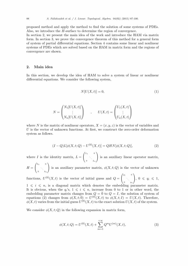
proposed method and apply the method to find the solution of some systems of PDEs.Also, we introduce the H-surface to determine the region of convergence.In section 2, we present the main idea of the work and introduce the HAM via matrixform. In section 3, we prove the convergence theorem of this method for a general formof system of partial differential equations. Section 4 contains some linear and nonlinearsystems of PDEs which are solved based on the HAM in matrix form and the regions ofconvergence are shown.

2. Main idea

In this section, we develop the idea of HAM to solve a system of linear or nonlineardifferential equations. We consider the following system,

N [U(X, t)] = 0, (1)

N =

N1[U(X, t)]...

Nn[U(X, t)]

, U(X, t) =

U1(X, t)...

Un(X, t)

where N is the matrix of nonlinear operators, X = (x, y, z) is the vector of variables andU is the vector of unknown functions. At first, we construct the zero-order deformationsystem as follows.

(I −Q)L[ϕ(X, t;Q)− U (0)(X, t)] = QHN [ϕ(X, t;Q)], (2)

where I is the identity matrix, L =

(L1 0

...

0 Ln

)is an auxiliary linear operator matrix,

H =

(h1 0

...

0 hn

)is an auxiliary parameter matrix, ϕ(X, t;Q) is the vector of unknown

functions, U (0)(X, t) is the vector of initial guess and Q =

(q1 0

...

0 qn

), 0 ⩽ qi ⩽ 1,

1 ⩽ i ⩽ n, is a diagonal matrix which denotes the embedding parameter matrix.It is obvious, when the qi’s, 1 ⩽ i ⩽ n, increase from 0 to 1 or in other word, theembedding parameter matrix changes from Q = 0 to Q = I, the solution of system ofequations (2) changes from ϕ(X, t; 0) = U (0)(X, t) to ϕ(X, t; I) = U(X, t). Therefore,ϕ(X, t) varies from the initial guess U (0)(X, t) to the exact solution U(X, t) of the system.

We consider ϕ(X, t;Q) in the following expansion in matrix form,

ϕ(X, t;Q) = U (0)(X, t) +

+∞∑m=1

QmU (m)(X, t), (3)

A. Fallahzadeh et al. / J. Linear. Topological. Algebra. 04(02) (2015) 87-100. 89

where

U (m)(X, t) =1

m!

∂mϕ1(X,t,q1)

∂qm1|q1=0

...∂mϕn(X,t,qn)

∂qmn|qn=0.

. (4)

The convergence of the vector series (3) depends upon the auxiliary parameter matrixH, if it is convergent at Q = I, we have

U(X, t) = U (0)(X, t) +

+∞∑m=1

U (m)(X, t). (5)

Now, we define the vector,

−→U k = {U (0)(X, t), . . . , U (k)(X, t)}, (6)

where,

U (i) =

U(i)1 (X, t)

...

U(i)n (X, t)

, i = 0, . . . , k. (7)

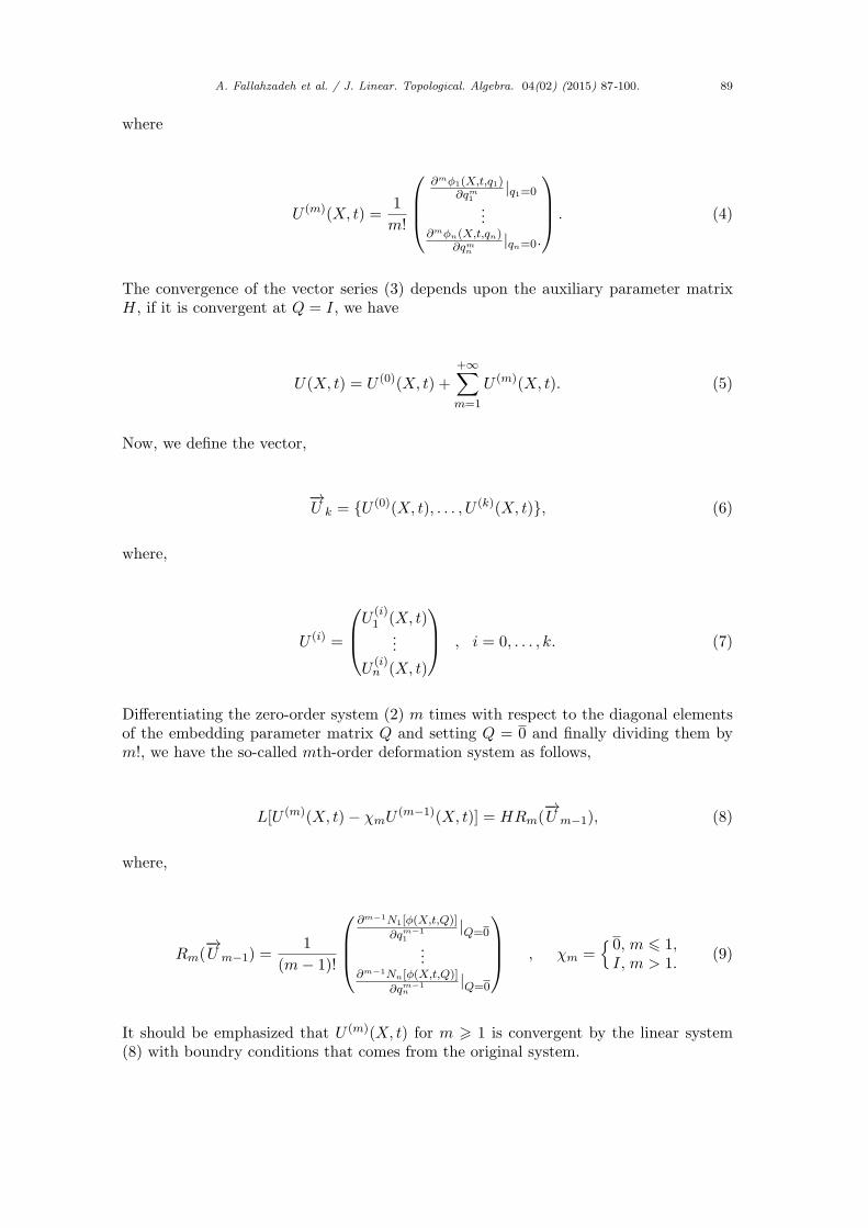
Differentiating the zero-order system (2) m times with respect to the diagonal elementsof the embedding parameter matrix Q and setting Q = 0 and finally dividing them bym!, we have the so-called mth-order deformation system as follows,

L[U (m)(X, t)− χmU (m−1)(X, t)] = HRm(−→U m−1), (8)

where,

Rm(−→U m−1) =

1

(m− 1)!

∂m−1N1[ϕ(X,t,Q)]

∂qm−11

|Q=0

...∂m−1Nn[ϕ(X,t,Q)]

∂qm−1n

|Q=0

, χm ={0, m ⩽ 1,I, m > 1.

(9)

It should be emphasized that U (m)(X, t) for m ⩾ 1 is convergent by the linear system(8) with boundry conditions that comes from the original system.


3. Convergence of the HAM for system of PDEs

In this case, we consider the following general form of the system of partial differentialequations,

ADS +BT +B′T ′ = C, (10)

where A is the 3× 3 coefficients matrix, D is the 3× 3 differential operator matrix that

[D]ij =∂α

(1)ij

∂xα(1)ij

+∂α

(2)ij

∂yα(2)ij

+∂α

(3)ij

∂zα(3)ij

+∂α

(4)ij

∂tα(4)ij

S is unknowns vector(u v w

)T. B and B′ are the 3 × 9 and 3 × 7 coefficients matrices

of functions respectively and T and T ′ are the following vectors:

T =(u v w u2 v2 w2 uv uw vw

)TT ′ =

(uv2 uw2 vu2 vw2 wu2 wv2 uvw

)Tand C =

(c1(x, y, z, t) c2(x, y, z, t) c3(x, y, z, t)

)Tis the 3× 1 vector of known functions.

In this part, we prove a theorem for convergence of the HAM for system of partialdifferential equations (10).

Theorem 3.1 If the series solution (5) of system (10) and also the series∑+∞

m=0DSm

where Sm =(um vm wm

)Tare convergent then the series (5) converges to the exact

solution of the system (10).

Proof. Let:

S =

+∞∑m=0

Sm,

where

limm→+∞

Sm =−→0 . (11)

We write

n∑m=1

[Sm − χmSm−1] = S1 + (S2 − S1) + (S3 − S2) + · · ·+ (Sn − Sn−1) = Sn.

Using (11), we have,

+∞∑m=1

[um − χmSm−1] = limn→+∞

Sn =−→0 .


According to the definition of the operator L, we can write

+∞∑m=1

L[Sm − χmSm−1] = L

+∞∑m=1

[Sm − χmSm−1] =−→0 .

From above expression and equation (8), we obtain

+∞∑m=1

L[Sm − χmSm−1] = H

+∞∑m=1

[Rm(−→S m−1)].

Since H ̸= 0, we have

+∞∑m=1

[Rm(−→S m−1)] =

−→0 . (12)

From (12), it holds

+∞∑m=1

Rm(−→S m−1) =

+∞∑m=1

ADSm−1

+B

+∞∑m=1

( (um−1 vm−1 wm−1

)T∑m−1i=0

(um−1um−1−i vm−1vm−1−i wm−1wm−1−i um−1vm−1−i um−1wm−1−i vm−1wm−1−i

)T)

+B′+∞∑m=1

m−1∑i=0

m−i−1∑k=0

( (uivkvm−i−k−1 uiwkwm−i−k−1 viukum−i−k−1

)T(viwkwm−i−k−1 wiukum−i−k−1 wivkvm−i−k−1 uivkwm−i−k−1

)T)

−(I − χm)C =−→0 .

We consider the following element from previous matrix equation. The similar manipu-lations can be done for other elements.


+∞∑m=1

m−1∑i=0

m−i−1∑k=0

uivkwm−i−k−1

=

+∞∑i=0

m−1∑m=i+1

m−i−1∑k=0

uivkwm−i−k−1

=

+∞∑i=0

ui

+∞∑m=i+1

m−i−1∑k=0

vkwm−i−k−1

=

+∞∑i=0

ui

+∞∑m=1

m−1∑k=0

vkwm−k−1

=

+∞∑i=0

ui

+∞∑k=0

+∞∑m=k+1

vkwm−k−1

=

+∞∑i=0

ui

+∞∑k=0

vk

+∞∑m=0

wm.

In addition, we have,

+∞∑m=1

ADSm−1 = AD

+∞∑m=0

Sm,

+∞∑m=1

(I − χm)C = C.

Therefore

ADS +BT +B′T ′ − C =−→0 . (13)

■

4. Test Examples

In this part, we consider three sample systems of PDEs and apply the matrix form ofHAM mentioned in previous section to solve these systems. The results in the tables havebeen provided by MAPLE.

Example 4.1 We consider the following linear system of PDEs:

utt + vx + 2u = 0,uxx + vt + 2u = 0,

(14)

with the initial conditions:


u(x, 0) = sin(x),ut(x, 0) = cos(x),v(x, 0) = cos(x).

(15)

The exact solution of this system is:

S(x, t) =

(sin(x+ t)cos(x+ t)

). (16)

We see:

N [S(x, t)] =

(N1[S(x, t)]N2[S(x, t)]

)=

(utt + vx + 2uuxx + vt + 2u

),

S(x, t) =

(u(x, t)v(x, t)

).

(17)

To solve the system (14) by means of HAM, we have:

N [ϕ(x, t,Q)] =

(N1[ϕ(x, t,Q)]N2[ϕ(x, t,Q)]

)=

(∂2ϕ1(x,t,q1)

∂t2 + ∂ϕ2(x,t,q2)∂x + 2ϕ1(x, t, q1)

∂2ϕ1(x,t,q1)∂x2 + ∂ϕ2(x,t,q2)

∂t + 2ϕ1(x, t, q1)

), (18)

where Q =(q1 00 q2

)and the linear matrix operator

L[ϕ(x, t,Q)] =

(∂2

∂t2 0

0 ∂∂t

)(ϕ1(x, t, q1)ϕ2(x, t, q2)

), (19)

with the property

L

(c1(x) + c2(x)t

c3(x)

)= 0, (20)

where c1(x), c2(x) and c3(x) are the integration constants. By using (8) under the initialconditions, we have:

Rm(−→u m−1) =

(∂2um−1(x,t)

∂t2 + ∂vm−1(x,t)∂x + 2um−1(x, t)

∂2um−1(x,t)∂x2 + ∂vm−1(x,t)

∂t + 2um−1(x, t)

). (21)

The solution of the mth-order deformation system (8) for m ⩾ 1 becomes:


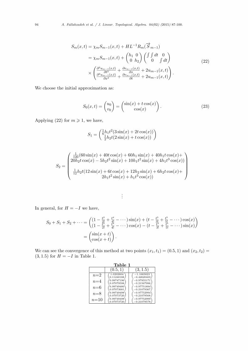
Sm(x, t) = χmSm−1(x, t) +HL−1Rm(−→S m−1)

= χmSm−1(x, t) +

(h1 00 h2

)(∫ ∫dt 0

0∫dt

)

×

(∂2um−1(x,t)

∂t2 + ∂vm−1(x,t)∂x + 2um−1(x, t)

∂2um−1(x,t)∂x2 + ∂vm−1(x,t)

∂t + 2um−1(x, t)

).

(22)

We choose the initial approximation as:

S0(x, t) =

(u0v0

)=

(sin(x) + t cos(x)

cos(x)

). (23)

Applying (22) for m ⩾ 1, we have,

S1 =

(16h1t

2(3 sin(x) + 2t cos(x))12h2t(2 sin(x) + t cos(x))

)

S2 =

1

120(60 sin(x) + 40t cos(x) + 60h1 sin(x) + 40h1t cos(x)+20h2t cos(x)− 5h2t

2 sin(x) + 10h1t2 sin(x) + 4h1t

3 cos(x))

112h2t(12 sin(x) + 6t cos(x) + 12h2 sin(x) + 6h2t cos(x)+

2h1t2 sin(x) + h1t

3 cos(x))

...

In general, for H = −I we have,

S0 + S1 + S2 + · · · =((1− t2

2! +t4

4! − · · · ) sin(x) + (t− t3

3! +t5

5! − · · · ) cos(x)(1− t2

2! +t4

4! − · · · ) cos(x)− (t− t3

3! +t5

5! − · · · ) sin(x)

)=

(sin(x+ t)cos(x+ t)

).

We can see the convergence of this method at two points (x1, t1) = (0.5, 1) and (x2, t2) =(3, 1.5) for H = −I in Table 1.

Table 1(0.5, 1) (3, 1.5)

n=2(

1.02026040.11240188

) (−1.1665823−0.42620403

)n=4

(0.997471960.07079598

) (−0.97955171−0.21567996

)n=6

(0.997494800.07073681

) (−0.97751894−0.21079367

)n=8

(0.997494980.07073720

) (−0.97752994−0.21079568

)n=10

(0.997494980.07073720

) (−0.97752999−0.21079578

)


We present the H-surfaces of the example 4.1 which is a two-dimensional system tosee the convergent region. In [8] the concept of h-curve was discussed to show the regionof convergence in the HAM to solve a given linear or nonlinear equation, where h is theauxilary parameter. These curves convert to surfaces for a set of equations like a systemof PDEs. By ploting the H-surface, it is easy to discover the valid region of the HAMand the optimal values of the entries of matrix H, which corresponds to the hyperplaneparallel to the hyperplane that is made by the h1, . . . , hn.In figures 1, 2 and 3, we plot the 5-approximation of u, v, vt, vx, utt and uxx when x = 0.5and t = 1. In this case, when H = −I we obtain the Taylor series of the exact solutionof the system. In this figures, we can see the region of convergence of the u, v, vt, vx, uttand uxx is [−2, 1]× [−2, 1].

Example 4.2 We consider the following linear system of PDEs with variable coefficients:

ut + vzz − wxx − u = 0,uyy + vtt − exwxx − v = 0,eyuyy + vxx − wttt − w = 0,

(24)


u(x, y, z, 0) = y + z,v(x, y, z, 0) = y + x,vt(x, y, z, 0) = y + x,w(x, y, z, 0) = x+ y,wt(x, y, z, 0) = x+ y,wtt(x, y, z, 0) = x+ y.

(25)


S(x, y, z, t) =

(y + z)et

(x+ z)et

(x+ y)et

. (26)

Similar to the example 4.1, for m ⩾ 1 we have:

Sm(x, y, z, t) = χmSm−1(x, y, z, t) +HL−1Rm(−→S m−1) = χmSm−1(x, y, z, t)

+

h1 0 00 h2 00 0 h3

×

∫ dt 0 00∫ ∫

dt 00 0

∫ ∫ ∫dt

×

∂um−1(x,y,z,t)

∂t + ∂2vm−1(x,y,z,t)∂z2 − ∂2wm−1(x,y,z,t)

∂x2 − um−1(x, y, z, t)∂2um−1(x,y,z,t)

∂y2 + ∂2vm−1(x,y,z,t)∂t2 − ex ∂2wm−1(x,y,z,t)

∂x2 − vm−1(x, y, z, t)

ey ∂2um−1(x,y,z,t)∂y2 + ∂2vm−1(x,y,z,t)

∂x2 − ∂3wm−1(x,y,z,t)∂t3 − wm−1(x, y, z, t)

.

(27)where


L =

∂∂t 0 0

0 ∂2

∂t2 0

0 0 ∂3

∂t3

, (28)

with the property

L

c1(x, y, z)c2(x, y, z) + c3(x, y, z)t

c4(x, y, z) + c5(x, y, z)t+ c6(x, y, z)t2

= 0, (29)

where c1(x, y, z), . . . , c6(x, y, z) are integration constant.

We choose the initial approximation as:

S0(x, y, z, t) =

u0v0w0

=

y + z(x+ z)(1 + t)

(x+ y)(1 + t+ 12 t

2)

. (30)

Applying (27) for m ⩾ 1 and H = −I we have,

S1 =

t(y + z)

( t2

2! +t3

3! )(x+ z)

( t3

3! +t4

4! +t5

5! )(x+ y)

S2 =

t2

2! (y + z)

( t4

4! +t5

5! )(x+ z)

( t6

6! +t7

7! +t8

8! )(x+ y)

...

In general, we have,

S0 + S1 + S2 + · · · =

(1 + t+ t2

2 + · · · )(x+ z)

(1 + t+ t2

2 + · · · )(y + z)

(1 + t+ t2

2 + · · · )(x+ z)

=

et(y + z)et(x+ z)et(x+ y)

.

We can see the convergence of this method at two points (x1, y1, z1, t1) = (1, 2, 3, 0.5)and (x2, y2, z2, t2) = (2, 3, 1, 3) for H = −I in Table 2.

Table 2


(1, 2, 3, 0.5) (2, 3, 1, 3)

n=28.1250000

6.59479174.9461639

34.0000000055.20000000100.0457589

n=4

8.24218756.59488514.9461639

65.5000000060.19017857100.4276173

n=6

8.24359816.59488514.9461639

77.6500000060.25640578100.4276846

n=8

8.24360646.59488514.9461639

80.0366071460.25661055100.4276846

n=10

8.24360646.59488514.9461639

80.3186607160.25661077100.4276846

Example 4.3 We consider the nonlinear system of ordinary differential equations asfollows:

utt − 2uv2 = 0,vt − uv = 0,

(31)


u(0) = 0,ut(0) = 1,v(0) = 1.

(32)


S(t) =

(tan(t)sec(t)

). (33)

In this example, we have:

N [ϕ(t,Q)] =

(N1[ϕ(t,Q)]N2[ϕ(t,Q)]

)=

(∂2ϕ1(t,q1)

∂t2 − 2ϕ1(t, q1)ϕ22(t, q2)

∂ϕ2(t,q2)∂t − ϕ1(t, q1)ϕ2(t, q2)

), (34)

where Q =(q1 00 q2

)and the linear matrix operator

L[ϕ(t,Q)] =

(∂2

∂t2 0

0 ∂∂t

)(ϕ1(x, t, q1)ϕ2(x, t, q2)

), (35)

with the property

L

(c1 + c2t

c3

)= 0, (36)

where c1, c2 and c3 are the integration constant. The solution of the mth-order deforma-tion system (8) for m ⩾ 1 becomes:


Sm(t) = χmSm−1(t) +HL−1Rm(−→S m−1) = χmSm−1(t) +

(h1 00 h2

)(∫ ∫dt dt 00

∫dt

)×(

∂2Sm−1(t)∂t2 − 2

∑+∞m=1

∑m−1i=0

∑m−i−1k=0 ui(t)vk(t)vm−i−k−1(t)

∂um−1(t)∂t −

∑+∞m=1

∑m−1i=0 ui(t)vm−i−1(t)

).

(37)We choose the initial approximation as:

S0(t) =

(u0v0

)=

(t1

). (38)

Applying (37), we can see the results of the method at two points t1 = 0.5 and t2 = 1for H = −I in Table 3.

Table 3

t1 = 0.5 t2 = 1n=2

(0.5458333341.138020833

) (1.466666671.708333333

)n=4

(0.54629767421.139478798

) (1.5425044091.827405754

)n=6

(0.54630244051.139493772

) (1.5549597731.846970484

)n=8

(0.54630248941.139493926

) (1.5570056351.850184116

)n=10

(0.54630248991.139493927

) (1.5573416791.850711974

)

5. Conclusion

In this work, the homotopy analysis method was introduced in matrix form and appliedto obtain the approximate solution of a linear or nonlinear system of partial differentialequations. For this purpose, a convergence theorem was proved and some sample systemsof PDEs were solved and the convergence of the HAM was discussed in each system.Also, the H-surface was introuced to illustrate the region of convergence in the HAM.Therefore, the HAM is able to solve the system of PDE via the matrix form and theconvergence of method is guranteed.

Aknowledgements

The authors are thankful to the Islamic Azad University, central Tehran branch for theirsupports during this research and also the anonymous referee for careful reading andsuggestion to improve the quality of this work.

References

[1] S. Abbasbandy, Homotopy analysis method for the Kawahara equation, Nonlinear Analysis: Real WorldApplications 11 (2010) 307-312.

[2] S. Abbasbandy, Solitary wave solutions to the modified form of CamassaHolm equation by means of thehomotopy analysis method, Chaos, Solitons and Fractals 39 (2009) 428-435.


[3] J. Biazar, M. Eslami, A new homotopy perturbation method for solving system of partial differential equa-tions, Computers and Mathematics with Applications 62 (2011) 225-234.

[4] J. Biazar, M. Eslami, H. Ghazvini, Homotopy perturbation method for system of partial differential equations,International Journal of Nonlinear Sciences and Numerical simulations 8 (3) (2007) 411-416.

[5] M.A. Fariborzi Araghi, A. Fallahzadeh, On the convergence of the Homotopy Analysis method for solvingthe Schrodinger Equation, Journal of Basic and Applied Scientific Research 2(6) (2012) 6076-6083.

[6] M.A. Fariborzi Araghi, A. Fallahzadeh, Explicit series solution of Boussinesq equation by homotopy analysismethod, Journal of American Science, 8(11) (2012).

[7] T. Hayat, M. Khan, Homotopy solutions for a generalized second-grade fluid past a porous plate. NonlinearDyn 42 (2005) 395-405.

[8] S.J. Liao, Beyond pertubation: Introduction to the homotopy Analysis Method, Chapman and Hall/CRCPress, Boca Raton, (2003).

[9] S.J. Liao, Notes on the homotopy analysis method: some definitions and theorems, Communication in Non-linear Science and Numnerical Simulation, 14 (2009) 983-997.

[10] P. Roul, P. Meyer, Numerical solution of system of nonlinear integro-differential equation by Homotopyperturbation method, Applied Mathematical Modelling 35 (2011) 4234-4242.

[11] A. Sami Bataineh, M.S.M. Noorani, I.Hashim, Approximation analytical solution of system of PDEs byhomotopy analysis method, Computers and Mathematics with Applications 55 (2008) 2913-2923.

[12] F. Wang, Y. An, Nonnegative doubly periodic solution for nonlinear teleghraph system, J.math.Anal.Appl.338 (2008) 91-100.

[13] A.M. Wazwaz, The variational iteration method for solving linear and nonlinear system of PDEs, Comput,Math, Appl 54 (2007) 895-902.

[14] W. Wu, Ch. Liou, Out put regulation of two-time-scale hyperbolic PDE systems, Journal of Process control11 (2001) 637-647.

[15] W. Wu, S. Liao, Solving solitary waves with discontinuity by means of the homotopy analysis method. Chaos,Solitons & Fractals, 26 (2005) 177-185.

[16] E. Yusufoglu, An improvment to homotopy perturbation method for solving system of linear equations,Computers and Mathematic with Applications 58 (2009) 2231-2235.


(a) H-surface of u (b) H-surface of v

Figure 1. H-Surfaces of u and v in example 4.1

(a) H-surface vt (b) H-surface vx

Figure 2. H-Surfaces of vt and vx in example 4.1

(a) H-surface utt (b) H-surface uxx

Figure 3. H-Surfaces of utt and uxx in example 4.1

On the convergence of the homotopy analysis method to...

Documents

Transcript of On the convergence of the homotopy analysis method to...