On the continuity of the equilibrium price density and its uses · 2017-04-12 · On the continuity...

On the continuity of the equilibrium price densityand its uses

Anthony Horsley and Andrew J. WrobelDepartment of Economics, London School of EconomicsHoughton Street, London WC2A 2AE, United Kingdom

(e-mail: [email protected])

3 March 2005CDAM Research Report LSE-CDAM-2005-04

Abstract

With L∞ as the commodity space, the equilibrium price density is shown tobe a continuous function of the commodity characteristics. The result is basedon symmetry ideas from the Hardy-Littlewood-Pólya theory of rearrangements. Itincludes, but is not limited to, the case of symmetric (rearrangement-invariant) pro-duction costs and additively separable consumer utility. For example, in continuous-time peak-load pricing of electricity, it applies also when there is a storage tech-nology and demands are cross-price dependent. In this context, a continuouslyvarying price has two uses. First, it precludes demand jumps that would arise fromdiscontinuous switches from one price rate to another. Second, in the problemsof operating and valuing hydroelectric and pumped-storage plants (studied else-where), price continuity guarantees that their capacities (viz., the reservoir and theconverter), the energy stocks, and in the case of hydro also the river flows, havewell-defined marginal values.

Keywords: Price continuity, equilibrium existence, efficiency rents, energy stor-age.2000 AMS Mathematics Subject Classification: Primary 91B50. Secondary

46E30.1991 Journal of Economic Literature Classification: C62, D51, D58, L94.

1

1 Introduction

Discontinuous pricing, e.g., in time-of-use (TOU) tariffs, is likely to result in disequilib-rium by creating demand discontinuities that are incompatible with pricing at marginalcost: e.g., with a sudden price drop, any consequential demand jump means that themarginal cost also rises and thus begins to differ from the ruling price. To avoid this,an equilibrium price must be continuous as a function of time. This property has otheruseful implications: for example, with marginal cost pricing of electricity, price continu-ity guarantees that the short-run profit function is differentiable in the fixed inputs, andhence that their efficiency rents are uniquely defined: see [15] or [18], and [16, Theorem1] or [17].1 And these values are fundamental to the short-run approach to long-runequilibrium that we develop in [20].When both demand and supply are cross-price independent, the price-continuity re-

sult can be obtained by the elementary method of supply and demand curves: theirintersection varies continuously with time if the curves do. This applies to, e.g., the caseof cross-price independent demand for electricity supplied by thermal plants (Section 2).By exploiting the results of [15] or [18], the method of curves can be extended to in-clude energy storage (Section 3). This is useful because, as we show in [15] or [18], pricecontinuity guarantees that the capacities of a storage plant (viz., the reservoir and theconverter) have definite marginal values.An alternative and ultimately much more general method of proving price continuity

in equilibrium begins by observing that, in examples like thermal electricity generation,the short-run supply curve remains unchanged over the cycle, which is represented bythe interval [0, T ]. So, on the assumption of no start-up or shutdown costs, the short-run cost is a symmetric (a.k.a. rearrangement-invariant) function of the output bundle y= (y (t))t∈[0,T ]–and hence so is the long-run cost. Symmetry means that the productioncost, C (y), depends on the values of y but not on their particular arrangement on [0, T ].In the language of electricity suppliers, the cost is a function of the load-duration curve,which mathematically is the decreasing rearrangement of y (Definition 5). Cost symme-try is useful because it implies that the trajectories of output y and of the supportingprice p are similarly arranged (Lemma 9 with Remark 10), which means that it cannotbe that p (t0) y (t00). With symmetry, this holds globally on [0, T ],i.e., for any instants t0 and t00. But, on the production side, it suffices to impose a weaker,local condition which formalises the notion that a price jump cannot entail a drop insupply (Definition 11). On the demand side, a similar, though slightly stronger, condi-tion means that a price jump must entail a drop in demand (Definition 22). Together,these conditions rule out a price jump in equilibrium (Theorem 26). The assumption onconsumer demand captures more than just the case of additively separable utility, and

1For the profit to be differentiable, the price does not have to be a pure density function: it sufficesthat the density part be continuous [15]. This is useful when the price contains also a “singular” part.

2

thus goes beyond the case of independent demands (Example 24). The assumption aboutsupply generalises both the case of symmetric costs and the case of additively separablecosts, but it has to be weakened further to include technologies such as energy storage(Definition 14 and Lemma 35).2

Although our analysis is motivated by a continuous-time problem, it applies to anygood differentiated by a commodity characteristic that ranges over a topological space,denoted also by T , which carries an “underlying” measure σ and thus generalises theinterval [0, T ] with the Lebesgue measure (for example, σ could be a probability on a“continuum” of events). In such a context, quantities of goods and their values areintegrals with respect to (w.r.t.) σ–and so the commodity space consists of functions,from T into the real line R, that are integrable, square-integrable or bounded (dependingon the problem). It must be paired with a suitable price space. A pair of Lebesguespaces, L% and L%

0with (1/%) + (1/%0) = 1, is an example; and the price space L%

0is the

norm-dual of L% when % < +∞.But the case relevant for peak-load pricing is that of % = +∞: the functions repre-

senting commodity bundles must be bounded because the problem involves capacity costsor constraints. The norm-dual of L∞ [0, T ] is larger than L1 [0, T ], and the elements ofL∞∗ \L1, called “price singularities”, have an essential role as capacity charges when theoutput y ∈ L∞ [0, T ] has a pointed peak: if the set {t : y (t) = Sup (y)} has zero Lebesguemeasure then the subdifferential ∂ Sup (y) lies wholly in L∞∗ \L1. When the equilibriumallocation actually lies in the smaller commodity space of continuous R-valued functions,C [0, T ], such a price functional can be restricted to C and represented by a singularmeasure. Thus it acquires a tractable mathematical form and can be used as part of aTOU tariff. For example, when the demand for electricity has a firm pointed peak, apoint measure represents the capacity charge in $ per kW demanded at the peak instant,whilst the fuel charge is a price density in $/kWh: see [14]. Thus the price system liesin the space of measuresM [0, T ].The type of equilibrium that the price space L1 [0, T ] does accommodate is one in

which the capacity charge is spread as a density over a peak plateau in the output. Suchan equilibrium arises if the users’ utility and production functions are Mackey continuous(which means that consumption is interruptible, i.e., that a brief interruption causes onlya small loss of utility or output): see [19]. For this case, we identify a set of conditions onwhich the equilibrium price function, p?, is not only integrable but also continuous. Theseconditions–viz., symmetry of production costs, additive separability of consumer utility,and their generalisations–are specific to commodity spaces of measurable functions (suchas L∞). Our price-continuity result is therefore quite different from those of Hindyet al. [7], Horsley [8] and [9], Jones [23], and Ostroy and Zame [28], which apply tothe commodity space of measuresM (T ), and therefore to a different class of problems

2Even in the context of thermal generation with storage, our general framework improves on themethod of curves because it applies also with interdependent demands.

3

(Section 10). They employ the standard approach to price representation, which reliesmainly on topological assumptions on consumer preferences and production sets in acommodity space paired with the “target” price space. When the price space is C (T ),that method necessitates the use ofM (T ) as the commodity space; so it could not serveour purposes because production costs such as the capacity cost are undefined outsidethe space L∞. However, like Ostroy and Zame, here as in [13] we exploit the “automatic”continuity of the essential limit, which reduces the task to showing that the limit of p?

exists everywhere on T .The method of curves, which does not require a fully formalised vector-space frame-

work, is presented first (Sections 2 and 3). The commodity and price spaces L∞ and L1

are introduced in Section 4. This is followed by a discussion of symmetry and its gener-alisations, in Sections 5 and 6. Section 7 gives the general price-continuity theorem. Thecase of additively separable utility (without cost separability) is spelt out in Section 8(with additional results showing that both price and quantity trajectories are continuousand bounded). The application to electricity pricing with storage and with a general,cross-price dependent demand is presented in Section 9, which extends and supersedesSection 3. Appendix A gives the proofs for Sections 5 to 9. Appendix B reviews theconcept of essential value (or limit). Appendix C reviews some properties of continuousfunctions.

2 Peak-load pricing with cross-price independent de-mands

The simplest model of equilibrium consists of supply and demand curves, S and D, in theprice-quantity plane; and if one or both curves vary continuously with a parameter suchas time, then so does their intersection point. This observation is useful in continuous-time peak-load pricing, i.e., pricing a cyclically demanded good which is produced by oneor more techniques with capacity costs (in addition to variable costs). In this context, acontinuous price can serve as an equilibrium solution to the problem of demand jumpscaused by discontinuous switches from one price rate to another in a TOU tariff. Alocal demand maximum arises on the wrong side of such an instant, viz., just after aprice drop (or just before a price jump). For example, the introduction of a two-ratetariff for electricity usually results in a surge of demand just after the switch from thedaytime rate to the night-time rate: see, e.g., [27, pp. 65—66 with Figure 2.2]. Since thisis a typical example, the cyclically priced flow in question is henceforth referred to aselectricity, although the model applies to other goods as well.With a one-station technology, the long-run marginal cost (LRMC) tariff has the

form p?LR (t) = w + rγ? (t), where r is the unit capacity cost, w is the unit runningcost, and γ? (with

Rγ? (t) dt = 1) is the distribution of the capacity charge, which is

4

concentrated on the (global) maxima of the long-run equilibrium output y?LR. To keepdemand constant during the peak, the price varies continuously with time. With a multi-station technology, the tariff structure is more complex: the offpeak price varies betweenthe lowest and the highest of the unit variable costs of the various station types. Marginalcost pricing means that the offpeak price is the generating system’s marginal variablecost, i.e., the unit fuel cost of the marginal station on line. (In the long run the systemmust also be optimal, i.e., it must minimise the total cost of meeting the demand.) Thusthe marginalist principle might appear to imply discontinuous price changes: with, say,a two-station technology with variable costs w1 < w2, it seems that the price must dropfrom w2 to w1 as soon as the demand (at price w2) has fallen to k1, the capacity ofthe first, base type. But the users’ response to such a sudden price drop is likely toreverse, albeit temporarily, the downward trend of demand–in which case, to meet thedemand at the price w1, the second station must immediately be switched back on, andthe marginal fuel cost increases back to w2. This undermines the tariff because the rulingprice, w1, differs from the marginal cost. And if the tariff is revised to take account ofthe new demand trajectory, new price discontinuities are created, so the difficulty arisesafresh. As we show, there is nevertheless an equilibrium solution: it consists in loweringthe price gradually, from w2 to w1, to keep the demand constant and equal to k1 for atime after the peak station has been switched off. The price keeps falling just enoughto maintain the demand (which would fall below k1 if the price were kept constant atw2). After such a transition period, the price “freezes” at w1, and demand starts fallingagain. Price and quantity move alternately (along the vertical and horizontal segmentsof the supply curve in Figure 1a), i.e., the price and output trajectories have alternatingplateaux: see Figures 1b and 1d.3 Thus price continuity implies that, in addition to thepeak plateau, the output has offpeak plateaux during which the price changes from w2to w1 and vice versa.In practice, a continuous price change could be approximated by a number of small

price jumps. A cruder but effective device is to stagger a price drop by timing it differentlyfor different consumers. For example, since 1977 Electricité de France has spread theonset of its night-time rate over one and a half hours;4 each consumer is notified of hisparticular night period but is given no choice in the matter. Since the effect on marketdemand is akin to facing the “average consumer” with a price varying between the tworates, this can be viewed as a rough implementation, workable even with two-rate orthree-rate meters, of the exact pricing solution.With a cross-price independent demand for electricity and a purely thermal generating3The graphs in Figures 1b and 1d are not periodic. They can be thought of in two ways: either as

representing only a part of the cycle, or as representing the whole cycle, but after a rearrangement oftime which produces nonincreasing price- and load-duration curves (and which exists by Lemma 9 andRemark 7).

4With a uniformly timed night-time rate, the EdF’s experience in 1976 was that demand would surge,just after the start of the low rate, by over 3GW (ca. 7% of maximum demand).

5

technology, the method of supply and demand curves applies directly to the short-runequilibrium, and it extends to the long-run equilibrium by the short-run approach. Theperfectly competitive short-run supply curve depends on the generating capacities (kθ)and their unit running costs (wθ), where θ = 1, . . . ,Θ are the various station types. Ifthe current electricity price is p, then the supply from station type θ is: Sθ (p) = 0 forp < wθ, Sθ (p) = kθ for p > wθ, and Sθ (p) = [0, kθ] for p = wθ (in which case Sθ (p) ismulti-valued). The total supply is STh (p) =

PΘθ=1 Sθ (p). For, say, Θ = 2 with w1 < w2,

the total supply from a two-station thermal system k = (k1, k2) is

STh (p) =

⎧⎪⎪⎪⎪⎨⎪⎪⎪⎪⎩0 for p < w1[0, k1] for p = w1k1 if w1 w2

(1)

(Figure 1a). This is, of course, the supply schedule of a producer whose short-run costis additively separable over the cycle [0, T ]. Here, for the thermal technology,

CSR (y (·)) =Z T

0

cSR (y (t)) dt (2)

with (see also Figure 1c)

cSR (y) =

Z y

0

S−1Th (q) dq =Z y

0

¡w11[0,k1] (q) + w21[k1,k1+k2] (q)

¢dq (3)

= w1y + (w2 − w1) (y − k1)+

if 0 ≤ y ≤ k1 + k2 (otherwise cSR = +∞).The demand Dt (p) is, at any time t, a function of the current price alone. It can be

interpreted as the demand of a household maximising the utility function

U (x (·) ,m) = m+Z T

0

u (t, x (t)) dt

over x (·) ≥ 0 andm ≥ 0 subject to the budget constraintm+R T0p (t) x (t) dt ≤M , where

M is the income and p (·) is a TOU price in terms of the numeraire (which represents allthe other goods and thus closes the model). With this behaviour, the equilibrium pricecan be expressed in terms of marginal utility and thus shown to be continuous in t if∂u/∂x is continuous. For each t, the instantaneous utility u (t, x) is taken to be a strictlyconcave, increasing and differentiable function of the consumption rate x ∈ R+, with(∂u/∂x) (t, 0) > w1 (to ensure that the short-run equilibrium demand is positive at everyt, if k1 > 0). For simplicity, all demand is assumed to come from a single household. Its

6

income M is the sum of an endowment of the numeraire (mEn) and the pure profit fromelectricity sales, i.e.,

M = mEn +2X

θ=1

µZ T

0

(p (t)− wθ)+ dt− rθ

¶· kθ

where r1 and r2 are the unit capacity costs (per cycle), and π+ = max {π, 0} is thenonnegative part of π. To guarantee a positive demand for the numeraire, assume thatmEn >

P2θ=1 (Twθ + rθ) kθ. Then the demand at any time t depends only on the current

price p (t), and it is determined from the equation

∂u

∂x(t, x (t)) = p (t) .

In other words, Dt (p) = ((∂u/∂x) (t, ·))−1 (p). When w2 < (∂u/∂x) (t, k1 + k2), thisvalue of ∂u/∂x is the price needed to equate demand to k1 + k2. Similarly, when w1≤ (∂u/∂x) (t, k1) ≤ w2, the middle term is the price needed to bring the demand downto k1. So the short-run equilibrium price can be given as

p?SR (t) = w1 +min

(µ∂u

∂x(t, k1)− w1

¶+, w2 − w1

)+

µ∂u

∂x(t, k1 + k2)− w2

¶+(4)

which is continuous in t if ∂u/∂x is (for any fixed x > 0). If additionally w1 >mint (∂u/∂x) (t, k1) and w2 < maxt (∂u/∂x) (t, k1), then those times t with p?SR (t) be-tween w1 and w2 (and with the equilibrium output equal to k1) form a set of positivemeasure.5 With k2 > 0, this is an offpeak plateau in the output (Figure 1d).The long-run equilibrium is obtained from the short-run equilibrium by solving the

simultaneous equations rθ =R T0(p?SR (t, k1, k2)− wθ)

+ dt for k and putting the solutionk? into p?SR (t, k).

6

The short-run price formula (4) extends to the case of any number, Θ, of stations.Also, no inequalities between the wθ’s need be assumed. This is useful when wθ dependson time, in which case there may be no fixed merit order among the stations. Denote byw↑ ∈ RΘ the nondecreasing rearrangement of the vector w = (wθ)

Θθ=1 ∈ RΘ (i.e., w↑1 is

the smallest entry in w, w↑2 is the second smallest, and so on). In these terms,

p?SR (t) = w↑1 (t) +

Θ−1Xθ=1

min

⎧⎨⎩⎛⎝∂u

∂x

⎛⎝t, Xα:wα(t)≤w↑θ (t)

kα

⎞⎠− w↑θ (t)⎞⎠+

,³w↑θ+1 (t)− w

↑θ (t)

´⎫⎬⎭(5)

5Note that 0 < meas {t : w1 < (∂u/∂x) (t, k1) < w2} because this set is nonempty and open.6In the case of a corner solution with k2 = 0, only the inequality r2 ≥

R T0(p?SR − w2)

+ dt holds.

7

+

Ã∂u

∂x

Ãt,

ΘXθ=1

kθ

!− w↑Θ (t)

!+.

3 Peak-load pricing with storage and independentdemands

In addition to eliminating demand jumps, price continuity is useful in the problem ofoperating and valuing storage facilities for cyclically priced goods. In the context ofelectricity this applies to hydroelectric and pumped-storage plants. Here we deal withpumped storage (PS); the case of hydro is similar. Unlike a thermal plant, a storageplant has two capital inputs, viz., the reservoir capacity kSt (in kWh) and the conversioncapacity kCo (in kW) which transforms the stored energy into electricity and vice versa.(For a more detailed description of the technology, see [18] and Section 9 here.) Givena TOU electricity price p and the plant’s capacities kPS = (kSt, kCo), the stock of energycan be assigned a TOU shadow price ψ (t), which is its marginal value in maximisationof the operating profit. As we show in [18, Lemma 8], ψ (t) is unique for every t if p (t) iscontinuous in t. In general, there is a set of such stock price functions Ψ (p, kPS), but ithas just one element, ψ (p, kPS), if p is continuous. It then follows that the capacities havedefinite and separate marginal values, and so does the river flow in the case of hydro: see[16, Theorem 1] and [17], in addition to [18, Theorem 9]. This brings out the importanceof price continuity in the general equilibrium.In terms of any ψ ∈ Ψ (p, kPS), the storage plant’s optimal output rate y (t) can be

given as in (6) below: y (t) = ±kCo if p (t) 6= ψ (t), with y (t) ∈ [−kCo, kCo] if p (t) = ψ (t).For each t, this defines the plant’s supply curve SPS,t in the price-quantity plane, butthe curve is not cross-price independent because it depends on ψ (t), which depends onthe whole function p. This means that, with a combined generation and storage system,the short-run equilibrium price cannot be found by intersecting curves as in the purelythermal case. Nevertheless, if p?SR is an equilibrium tariff, and St is the system’s supplycurve constructed from kθ, wθ, kCo and a ψ ∈ Ψ (p?SR, kPS), then–for a certain choice,ψ?SR, of ψ–the curve St intersects the demand curve Dt at p

?SR (t). This fact can still be

used to show that p?SR is continuous, but the argument requires an extra step, which is toshow that ψ?SR (t) is continuous in t (and hence that St varies continuously with t). Onceψ?SR is known to be continuous, continuity of p

?SR follows, as in the purely thermal case,

from (5), which is now applied with Θ+1 instead of Θ and with wΘ+1 (t) := ψ?SR (t). (Italso follows that the set Ψ (p?SR) is actually a singleton ψ (p?SR), and that this is ψ

?SR.)

It remains to show that ψ?SR is indeed continuous. This can be deduced from equi-librium conditions and two properties of every ψ ∈ Ψ, viz.: (i) that ψ is of boundedvariation, so it has the two one-sided limits ψ (t±),7 and (ii) that ψ rises or falls (possi-

7Since the set of t’s with ψ (t−) 6= ψ (t+) is at most countable, it does not matter which of the two

8

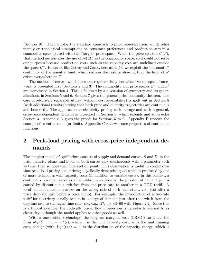
bly with a jump or a drop) only when the reservoir is full or empty, respectively. Considera system with, say, two thermal stations as in (1) and one storage station (with conversioncapacity kCo). With p?SR and ψ?SR abbreviated to p

? and ψ?, introduce the curve

SPS,t (p) =

⎧⎨⎩ −kCo for p < ψ? (t)[−kCo, kCo] for p = ψ? (t)kCo for p > ψ? (t)

(6)

and add it to the STh of (1) to form

St (p) = STh (p) + SPS,t (p) .

For every t, this curve intersectsDt at p? (t). When p? (t) = ψ? (t), the rate of equilibriumoutput from storage can be read off as the horizontal distance from the intersection pointto the centre of the horizontal segment of length 2kCo which St has at the price ψ? (t):see Figure 2. As the point is left or right of centre, so the output is negative or positive,i.e., the reservoir is being charged or discharged, respectively.Suppose that ψ? has a jump at some t, i.e., ψ? (t−) < ψ? (t+). Say there is no wθ

between ψ? (t−) and ψ? (t+). (If there is, it only helps the argument.) Figure 2 showsthe case of Θ = 2 with w1 < ψ? (t−) < ψ? (t+) < w2; the curve given by (1) plus (6)with ψ? (t−) or ψ? (t+) in place of ψ? (t) is denoted by St− or St+. Now note that Dtcannot intersect St+ below ψ? (t+) or to the left of centre of the horizontal segment atthe level ψ? (t+), since this would mean that the reservoir is being charged for a timejust after t, which is infeasible because the reservoir is full at t.8 Similarly, Dt cannotintersect St− above ψ? (t−) or to the right of centre of the horizontal segment at thelevel ψ? (t−), since this would mean that the reservoir is being discharged for a time justbefore t, which is again infeasible. (In Figure 2, the lines that Dt cannot intersect arethe heavy lines.) So, being monotone, Dt must have a vertical segment, from the centreat level ψ? (t+) to the centre at level ψ? (t−). But such a vertical segment contradictsthe strict monotonicity of Dt in p, i.e., the differentiability of u (t, ·). This shows that ψ?is continuous, and hence so is p?.In Section 9, continuity of p? (·) and ψ (p?) (·) is re-derived in a different way, and

in the other order: first it is proved for p? (by applying Theorem 26). And if p (·) iscontinuous then so is ψ (p) (·): see [15] or [18, Lemma 8].9

values is chosen for ψ (t) itself.8Continuity of Dt in t is used here.9Obviously that result cannot be used to derive the continuity of p? from that of ψ? as in this section:

such an argument would be circular.

9

4 Commodity and price spaces for a general frame-work

The method of curves is limited to the case of independent demands (Sections 2 and3). However, a more general price-continuity result can be based on the same ideathat a price jump would cause a drop in the demand trajectory but a jump in thesupply trajectory. The demand drop must be nonzero to include the case when supplydoes not actually jump but does not drop either–as can be the case in, e.g., thermalelectricity generation (see Figure 1a, where y stays at k1 if p jumps from w1 to w2).For a general result (Theorem 26), such responses of demand and supply to price jumpsare simply assumed. We name them sub-symmetry and quasi-symmetry of preferencesand technologies, since these properties follow from the stronger condition of symmetry,i.e., from invariance under rearrangement. A function C of y = (y (t))t∈[0,T ] is calledsymmetric (a.k.a. rearrangement-invariant) if C (y) depends only on the distribution ofy w.r.t. the Lebesgue measure on [0, T ].10 For example, the short-run cost of thermalelectricity generation, the CSR of (2), is symmetric, and so is its long-run cost (whichis not additively separable like CSR). When C is convex, its symmetry guarantees thaty and p = ∇C (y) are similarly arranged, i.e., that for (almost) every t0 and t00 if p (t0)< p (t00) then y (t0) ≤ y (t00): see [12, Theorem 1]. Applied to a joint cost as a functionof the output trajectory y, this means that outputs are always higher (or at least notlower) at higher-priced times. In other words, price and output increments do not haveopposite signs anywhere on [0, T ].Similarity of arrangement of prices and outputs is thus a global consequence of cost

symmetry. Its full strength is not necessary for proving price continuity, which is a localproperty of the equilibrium price function p?: [0, T ]→ R. It suffices to assume a local andapproximate version of the arrangement similarity between quantities and the supportingprices–and this is sub-symmetry (Definition 11). On the production side, the assumptionis further weakened to quasi-symmetry (Definition 14), to make it hold for technologiessuch as energy storage (Lemma 35). On the consumption side, the assumption is slightlystrengthened (Definition 22). It is verified for differentiable additively separable utility(Example 23); extensions to other forms of utility are sketched (Example 24). Theseresults (Lemma 35 and Example 23) make Theorem 26 apply to peak-load pricing ofelectricity with cross-price independent demands and with (or without) energy storage,thus re-establishing the results of Section 3 (and Section 2).Such an analysis requires the duality framework of a pair of function spaces to repre-

sent commodities and prices. In peak-load pricing, an output bundle is always boundedby the productive capacity, so the commodity space is L∞ [0, T ]. It is paired with L1 [0, T ]as the price space–but our task is to show that the equilibrium price density p? is con-10Equivalently, C is symmetric if C (y) = C (y ◦ ρ) for every Lebesgue measure-preserving transfor-

mation ρ: [0, T ]→ [0, T ].

10

tinuous (and not just integrable) on [0, T ]. Before this application, T standing alonedenotes an abstract set of commodities which carries a topology with a countable baseof open sets. Additionally, T carries a finite nonatomic (and nonnegative) measure σon a sigma-algebra A that contains all the Borel subsets of T . Every nonempty opensubset of T is assumed to be σ-nonnull, i.e., to have a positive measure. The vectorspace of all σ-equivalence classes of A-measurable real-valued functions on T is denotedby L0 (T,σ). The commodity space of all σ-essentially bounded functions, L∞ (T ), ispaired with L1 (T ), the price space of all σ-integrable functions.11

Apart from T (which may represent a single differentiated good), there is a finitenumber of homogeneous goods numbered by 1, 2, . . . , G ≥ 0. So a complete commoditybundle is a (y, q) ∈ L∞ (T )×RG, and its value at a price system (p, r) ∈ L1 (T )×RG isRTp (t) y (t)σ (dt) + r · q, abbreviated to hp | yi+ r · q.

5 Symmetry and weaker conditions on productionsets

We next formalise the idea that a jump in the price trajectory cannot coincide witha drop in the supply trajectory. First, this is shown to follow from symmetry of thecost function (or of the input correspondence when the inputs are not aggregated intoa scalar cost). Symmetry implies an even stronger “similarity” of the price and outputtrajectories, viz., that they rise and fall simultaneously (Lemma 9 and Remark 10). Thisis more than is actually needed for price continuity, and the assumption is too strongfor some applications: in electricity pricing, the cost of energy storage is not symmetric(although the cost of thermal generation is). We therefore weaken the similarity condition(Definitions 11, 14 and 17). Like symmetry, the weaker properties are preserved insummation of production sets. Some “general” examples meeting the weak conditionsare given at this stage, but the motivating example of energy storage is dealt with inSection 9 (Lemmas 35 and 37).

Definition 1 A function C on L0 (T ) is σ-symmetric (a.k.a. rearrangement-invariant)if, for every y and z in L0 (T ), the condition σ (y−1 (B)) = σ (z−1 (B)) for every Borel setB ⊂ R implies that C (y) = C (z). (In other words, C is symmetric if its value dependsonly on the distribution of its argument w.r.t. σ.)

Definition 2 A set S ⊂ L0 (T ) is σ-symmetric if its indicator function is symmetric,i.e., if the conditions: y ∈ S, z ∈ L0 and σ (y−1 (B)) = σ (z−1 (B)) for every Borel setB ⊂ R imply that z ∈ S also. (In other words, S is symmetric if z ∈ S whenever z hasthe same distribution, w.r.t. σ, as some y ∈ S.)11The analysis can be adapted for use with other L%-spaces in problems involving unbounded com-

modity bundles.

11

When this concept is used here, S is the section of a production set Y ⊂L∞ (T )×RGthrough a q ∈ RG, i.e., S is the q-restricted production set

Y (q) := {y ∈ L∞ (T ) : (y, q) ∈ Y} . (7)

The set of “output” bundles Y (q) is symmetric for each “input” q ∈ RG if and only ifthe “input requirement” set Yy := {q : (y, q) ∈ Y} depends only on the distribution of y.In such a case, the production cost

C (y) := infq{− hr | qi : (y, q) ∈ Y}

is a symmetric function of y (for each input price system r ∈ RG).For the purpose of proving price continuity on T , the relevant implication of symmetry

is similarity of arrangement for the functions p and y (on T ) which represent a pricesystem and an output bundle that maximises the (q-restricted) profit on S = Y (q). Thisresult (Lemma 9) is preceded by a discussion of similarity of arrangement, a conceptintroduced by Day [2, p. 932].

Definition 3 Two elements, p and y, of L0 (T ) are similarly arranged if, for any mea-surable sets A0 and A00,12

ess supA0p < ess inf

A00p⇒ ess sup

A0y ≤ ess inf

A00y. (8)

After replacing p and y by any of their variants p and y–which are literally functionsrather than equivalence classes of almost everywhere (a.e.) equal functions–similarityof arrangement can be usefully reformulated in terms of values at any points t0 and t00

(instead of values on sets A0 and A00).

Remark 4 Two elements, p and y, of L0 (T ) are similarly arranged if and only if

p (t0) < p (t00)⇒ y (t0) ≤ y (t00)

for σ-almost every (a.e.) t0 and t00 in T–i.e., if and only if for any variants p and y (ofp and y) there is a σ-null set Z such that for every t0 and t00 in T \ Z

p (t0) < p (t00)⇒ y (t0) ≤ y (t00) . (9)

As is shown by Day [2, p. 939, 5.6], similarity of arrangement is equivalent to theexistence of a common ranking pattern. To state this, we first introduce the concepts.12It obviously suffices to verify this for any σ-almost disjoint pair of σ-nonnull sets, A0 and A00.

12

Definition 5 The nonincreasing rearrangement y↓ of a y ∈ L0 (T,σ) is the nonincreasingfunction on [0,σ (T )] with the same distribution, relative to the Lebesgue measure (meas),as the distribution of y w.r.t. σ. That is, y↓ is nonincreasing and, for every Borel setB ⊂ R,13

meas {τ ∈ [0,σ (T )] : y↓ (τ) ∈ B} = σ {t ∈ T : y (t) ∈ B} .

Definition 6 A ranking pattern of a y ∈ L0 (T,σ) is any measure-preserving mapρ: T → [0,σ (T )] such that y = y↓ ◦ ρ. The set of all such maps is denoted by R (y).14

Comments:

1. R (y) 6= ∅ (if σ is nonatomic). This is the Lorentz-Ryff Lemma [31, Lemma 1],stated also in, e.g., [3, 3.3].

2. If y has no plateau (i.e., σ {t : y (t) = y} = 0 for each y ∈ R or, equivalently, y↓ isstrictly decreasing), then the pattern of y is unique, and it is

ρy = (y↓)−1 ◦ y.

Note that ρy (t) = σ {τ ∈ T : y (τ) ≥ y (t)}, i.e., ρy (t) /σ (T ) is t’s “percentageabove”–the fraction of T on which y is above its “current” value y (t). Thus ρyranks the elements of T by the value of y (hence its name, “the ranking pattern”).

Remark 7 (Day) Assume that σ is nonatomic (on A). Two functions p and y, inL0 (T,A,σ), are similarly arranged if and only if

R (p) ∩R (y) 6= ∅ (10)

i.e., if and only if both p = p↓ ◦ ρ and y = y↓ ◦ ρ for some measure-preserving mapρ: T → [0,σ (T )].

Comments:

1. It is obvious that (10) implies (9) or, equivalently, (8). To prove the converse–that(8) implies (10)–Day [2, p. 939, 5.6] shows that (8) implies that the pair (p, y)is jointly equidistributed to (p↓, y↓), i.e., that (p, y) has the same joint distributionas (p↓, y↓), and that this in turn implies (10). Thus he extends the Lorentz-RyffLemma to pairs (and also n-tuples) of functions, and adds the joint equidistributionas another equivalent condition.

13When y is the output and p is a TOU tariff, the graphs of y↓ and p↓ are known in electricity pricingas the load-duration and price-duration curves. On L∞, the operation x 7→ x↓ is m

¡L∞, L1

¢-continuous:

see [10].14“Measure-preserving” means that σ

¡ρ−1 (B)

¢= measB for every Borel set B ⊂ [0,σ (T )].

13

2. In (8) and (9), the inequalities in the antecedent and the consequent must be strictand nonstrict, respectively.

3. As is obvious from Remark 4 (or Remark 7), similarity of arrangement is a sym-metric binary relation in L0–i.e., p and y can be interchanged in (8) or (9). It isnot a transitive relation (since every function is arranged similarly to a constant).

As we note next, similarity of arrangement is preserved in summation.

Remark 8 If each of two functions, y and z, is arranged similarly to p, then so is y+z.

As has been mentioned, if p represents a linear functional supporting a symmetricset S at a point y, then p and y are similarly arranged (or, equivalently, have a commonpattern). This is next spelt out for the case of p ∈ L1 and y ∈ S ⊂ L∞. (The same holdsfor L% and L%

0instead of L∞ and L1.)

Lemma 9 Assume that the measure σ is nonatomic (on A) and that S is a symmetricsubset of L∞ (T,A,σ). If p ∈ L1 (T ) and y maximises hp | ·i on S–i.e., y ∈ S and hp | yi= sup {hp | zi : z ∈ S}–then p and y are similarly arranged.

The corresponding result for functions follows [12, Theorem 1].

Remark 10 If σ is nonatomic, C: L∞ (T,σ) → R is a symmetric convex function andp ∈ ∂C (y)∩L1 (T,σ), i.e., a p ∈ L1 is a subgradient of C at y, then p and y are similarlyarranged.

Applied to a (restricted) production set S = Y (q), Lemma 9 shows that, in an outputbundle y ∈ S ⊂ L∞ (T ) and a supporting price system p ∈ L1 (T ), the quantity and pricemove up and down together over “time”. But a weaker property, introduced next, sufficesfor the purpose of proving price continuity.

Notation The set of all neighbourhoods of t is denoted by N (t).

Definition 11 A set S ⊂ L∞ (T ) is sub-symmetric if: for every p ∈ L1 (T ) and everyy that maximises hp | ·i on S, and for every t ∈ T and ² > 0, there exists an H ∈ N (t)such that for any two measurable sets A0 ⊂ H and A00 ⊂ H

²+ ess supA0p < ess inf

A00p ⇒ ess sup

A0y ≤ ess inf

A00y. (11)

Equivalently, S is sub-symmetric if, for every p, y, t and ² such as above, there exists anH ∈ N (t) such that, for σ-almost every t0 and t00 in H,15

²+ p (t0) < p (t00)⇒ y (t0) ≤ y (t00) . (12)15As in Remark 4, the p and y in (12) must be interpreted as any variants p and y, and the phrase

“for a.e. t0 and t00 in H” is to be interpreted as meaning “for every t0 and t00 in H but outside of someσ-null set Z ”. The excepted set Z depends on the choice of variants p and y, but it can be chosenindependently of ² and, also, of t (since the topology of T has a countable open base).

14

Comments:

1. Unlike the case of a symmetric S, in which p and y are similarly arranged byLemma 9, if S is only sub-symmetric then the relationship between p and y is notsymmetric, i.e., p and y cannot be interchanged in (11) or (12).

2. Because of the ², the strict inequality between the values of p in the antecedent of(11) or (12) can be made nonstrict without changing the concept. But the inequalitybetween the values of y in the consequent of (11) or (12) must be non-strict, as in(8) or (9).

Every symmetric set is obviously sub-symmetric.16 A proper example of sub-symmetryin production is the additively separable convex cost

RTc (t, y (t)) dt: it is not a symmet-

ric function of y unless the “instantaneous” cost is independent of t directly (i.e., unlessthe integrand c (t, y) is actually independent of t, as in (2)). But if the cost curve c (t, ·),together with its y-derivative, varies continuously with t, then it can be approximated ina neighbourhood of any t0 ∈ T by the fixed (time-independent) curve c (t0, ·). This is whyRc (t, y (t)) dt is “locally and approximately” symmetric: in precise terms, its sublevel

sets are sub-symmetric, as is shown next.

Example 12 Assume that c: T × (−∞, k]→ R, where k ∈ R is a constant, is a differ-entiable convex integrand, i.e., the function t 7→ c (t, y) is σ-integrable on T (for everyy ∈ R), whilst the function y 7→ c (t, y) is convex and differentiable on (−∞, k], for everyt ∈ T . Then

C (y) :=

ZT

c (t, y (t))σ (dt) (13)

is a convex integral functional on L∞ (T ), defined effectively for y ≤ k: see, e.g., [29].If additionally ∂c/∂y is (jointly) continuous on T × (−∞, k] then, for every a ∈ R,

the setS = {y ∈ L∞ (T ) : C (y) ≤ a} (14)

is sub-symmetric, provided that C (y) < a for some y (Slater’s Condition).

Comments:

1. (∂c/∂y) (t, k) means the left (one-sided) derivative (w.r.t. y, at y = k); it is assumedto be finite.

16To satisfy (11) when S is symmetric, it suffices to set H = T regardless of ² (by Lemma 9 andDefinition 3).

15

2. With c differentiable in y on (−∞, k), even a strict inequality holds between thevalues of y in (12), except when y (t0) = y (t00) = k. The exception is caused bythe kink which c (t, ·) has at y = k (where the curve is “cut off” by setting c (t, y)= +∞ for y > k).

3. Typically, a negative y (t) can arise only from free disposal, and so the “instanta-neous” production cost c (t, y) is nondecreasing in y, with c (t, y) = 0 for y ≤ 0.In such a case, c (t, ·) usually has a kink at y = 0 but, like its kink at y = k,this does not spoil the sub-symmetry result: Example 12 extends to the case of(∂c/∂y) (t, 0+) > 0 = (∂c/∂y) (t, 0−).

Example 12 is next reoriented for application to an industrial customer, who uses adifferentiated input z ∈ L∞+ (T ) to produce a quantity

RTf (t, z (t)) dt of a homogeneous

output good.

Example 13 Assume that f : T × R+ → R is a differentiable concave integrand, i.e.,the function t 7→ f (t, z) is σ-integrable on T (for every z ∈ R), and that the functionz 7→ f (t, z) is concave and differentiable on R+. Then

F (z) :=

ZT

f (t, z (t)) σ (dt) (15)

is a concave integral functional on L∞+ (T ): see, e.g., [29].If additionally ∂f/∂z is (jointly) continuous on T ×R+ then, for every ζ ∈ R, the set

S =©−z ∈ L∞− (T ) : F (z) ≥ ζ

ª(16)

is sub-symmetric, provided that F (z) > ζ for some z (Slater’s Condition).

There is a significantly weaker condition on the technologies that, together with sub-symmetry of preferences, ensures price continuity in equilibrium. To formulate it, we usethe concept of the essential value of p at t. Denoted by ess p (t), it exists if and only if thelower and upper essential values, p (t) and p (t), are equal and finite. In other words, t/∈ domess p if and only if either −∞ < p (t) < p (t) < +∞ or p (t) = −∞ or p (t) = +∞.These concepts are reviewed in Appendix B.

Definition 14 A set S ⊂ L∞ (T,σ) is quasi-symmetric if: for every p ∈ L1 (T ) andevery y that maximises hp | ·i on S, and for any t‡ ∈ T \ domess p, there is a numberα > 0 such that every neighbourhood N ∈ N (t‡) has a pair of σ-nonnull subsets, A0 ⊂ Nand A00 ⊂ N , such that

α+ ess supA0p ≤ ess inf

A00p (17)

16

ess supA0y ≤ ess inf

A00y (18)

i.e., for σ-almost every t0 ∈ A0 and t00 ∈ A00,17

α+ p (t0) ≤ p (t00) (19)

y (t0) ≤ y (t00) . (20)

The “price part” (17) of the quasi-symmetry condition is always met because, as isnoted next, it follows purely from the hypothesis of a price discontinuity (i.e., from thenonexistence of ess p at t‡).

Remark 15 For any t‡ ∈ T \ domess p, there is an α > 0 such that every N ∈ N (t‡)has σ-nonnull subsets, A0 and A00, with α+ ess supA0 p ≤ ess infA00 p. More specifically:

1. If p (t‡) = −∞ or p (t‡) = +∞, then every α > 0 has this property.

2. If −∞ < p (t‡) < p (t‡) < +∞, then any positive α < p (t‡)−p (t‡) has this property.

Corollary 16 Every sub-symmetric set (and hence every symmetric set) is quasi-symmet-ric.

The next condition on the technologies does not come into the general price-continuityresult itself (Theorem 26). But it is needed to verify that, in equilibrium, the theorem’sstrong sub-symmetry assumption on consumer preferences holds in specific cases, suchas that of differentiable additively separable utility (Section 8). It serves to establishfirst that the equilibrium price function is bounded and that consumption is thereforebounded away from zero (which is necessary for strong sub-symmetry to hold). Thiscondition, formulated next, requires merely that the profit-maximising output must bearbitrarily close to its peak at the “times” of sufficiently high prices (if the price functionis unbounded).18

Definition 17 A set S ⊂ L∞ (T ) is pseudo-symmetric if, for every p ∈ L1 (T ) and everyy that maximises hp | ·i on S,

limp%+∞

ess inft: p(t)>p

y (t) ≥ EssSup (y) := ess supt∈T

y (t) (21)

i.e., if for every δ > 0 there is a p ∈ R such that, for σ-almost every t ∈ T ,

p (t) > p⇒ y (t) ≥ EssSup (y)− δ. (22)

17This means “for every t0 in A0 and t00 in A00 but outside of some σ-null set Z ”. The excepted set Zdepends on the choice of variants of p and y, but it can be chosen independently of N and t‡.18In the case of an industrial user, the condition means that his profit-maximising input must be

arbitrarily close to its minimum when the price is high, since his net output of the differentiated goodis, of course, the negative of his input.

17

Comment: The question arises only when p is unbounded: when p ∈ L∞, Condition(22) is met vacuously by p = EssSup (p) or larger (since this means that p (t) ≤ p for a.e.t). In other words, if p is bounded from above, then (21) holds for every y ∈ L∞ becausethe inequality in (21) has +∞ on its left-hand side; this is the only case in which theinequality in (21) is strict.

Lemma 18 Every symmetric set is pseudo-symmetric.

An industrial user of a differentiated good meets a pseudo-symmetry condition if hisproduction function is additively separable.19

Example 19 Under the assumptions of Example 13 on the concave functional F (z):=RTf (t, z (t))σ (dt) for z ∈ L∞+ (T ), if additionally supt∈T (∂f/∂z) (t, 0) < +∞ (as is

the case when T is compact and ∂f/∂z is continuous in t), then, for every ζ ∈ R, the setS = − {z ≥ 0 : F (z) ≥ ζ} is pseudo-symmetric (provided that F (z) > ζ for some z).

The “symmetry-like” concepts are applied to the sections of a production set Y ⊂L∞ (T ) × RG through a q ∈ RG. To say that such a set has symmetric T -sections (orsub-symmetric T -sections, etc.) means that, for every q ∈ RG, the set Y (q) definedby (7) is symmetric (or sub-symmetric). These properties are mostly preserved in thesummation of sets (although quasi-symmetry for the sum requires sub-symmetry for allbut one of the sets). To establish this, note first that

(Y0 +Y00) (q) =[

(q0,q00): q0+q00=q

(Y0 (q0) +Y00 (q00)) . (23)

Furthermore, the components of a profit-maximising output bundle in the sum’s sectionare also profit maxima: in precise terms, if

y = y0 + y00 maximises hp | ·i on Y (q) := (Y0 +Y00) (q) (24)

q = q0 + q00 and (y0, q0) ∈ Y0 and (y00, q00) ∈ Y00 (25)

theny0 maximises hp | ·i on Y0 (q0) and y00 maximises hp | ·i on Y00 (q00) . (26)

Lemma 20 If two subsets, Y0 and Y00, of L∞ (T )× RG have symmetric T -sections thatare additionally convex and w (L∞, L1)-closed (weakly* closed) in L∞ (T ), then also theirsum Y := Y0 +Y00 has symmetric sections.

Lemma 21 For any two subsets, Y0 and Y00, of L0 (T )×RG:19Similarly, a supplier of the good meets the pseudo-symmetry condition if his cost is additively

separable, as in Example 12.

18

1. If both Y0 and Y00 have sub-symmetric T -sections, then so has their sum Y :=Y0 +Y00.

2. If Y0 has quasi-symmetric sections, and Y00 has sub-symmetric sections, then theirsum Y := Y0 +Y00 has quasi-symmetric sections.

3. If both Y0 and Y00 have pseudo-symmetric sections, then so has their sum Y :=Y0 +Y00.

6 Sub-symmetry of preferences

A variant of the sub-symmetry concept is needed to formulate a condition on consumerpreferences which, together with quasi-symmetry of the production set, ensures pricecontinuity in equilibrium. For use in this context, the condition is reoriented to minimi-sation of “expenditure” instead of maximisation of “profit” as in Definition 11. Also, itis formulated “pointwise” because its verification requires a condition on the particularconsumption bundle x: Example 23 requires that Inf (x) > 0 (which is needed becausethe demand x (t) cannot drop when it is already zero). Recall that N (t) means the setof all neighbourhoods of t.

Definition 22 A set S ⊂ L∞ (T ) is strongly sub-symmetric at a point x ∈ S if: forevery p ∈ L1 (T ) such that x minimises hp | ·i on S, and for every t ∈ T and ² > 0, thereexist an H ∈ N (t) and a δ > 0 such that, for any two measurable sets A0 ⊂ H andA00 ⊂ H,

²+ ess supA0p < ess inf

A00p ⇒ ess inf

A0x ≥ δ + ess sup

A00x. (27)

Equivalently, S is strongly sub-symmetric at x if, for any t and ² such as above, thereexists an H ∈ N (t) and a δ > 0 such that, for σ-almost every t0 and t00 in H,

²+ p (t0) < p (t00)⇒ x (t0) ≥ x (t00) + δ. (28)

Comment: A symmetric set need not be strongly sub-symmetric at every point. Forexample, if c (t, y (t)) in (13) is actually c (y (t)), a convex function of y (t) alone, thenthe sublevel set (14) is symmetric and hence sub-symmetric, but not strongly so (at apoint x = −y), unless c is differentiable and EssSup (y) < k.This concept is used with S equal to a superlevel set for the ordering of L∞+ (T )

obtained by fixing an em ∈ RG in an ordering 4 of L∞+ (T )×RG+, i.e., with S equal toS (ex, em,4) := ©x ∈ L∞+ (T ) : (ex, em) 4 (x, em)ª (29)

which is a “preferred set” for the section of 4 through em. When 4 is represented by afunction U on L∞+ (T ) × RG+, this set is {x : U (ex, em) ≤ U (x, em)}, a superlevel set of U= U (·, em).

19

In the following example of strong sub-symmetry in consumption, the utility functionhas the additively separable form, U (x) =

RTu (t, x (t)) dt. This is mathematically sim-

ilar to the case of additively separable cost and production functions (Examples 12 and13).

Example 23 Assume that u: T × R+ → R is a differentiable concave integrand, i.e.,the function t 7→ u (t, x) is σ-integrable on T (for every x ∈ R+), whilst the functionx 7→ u (t, x) is concave, (strictly) increasing and differentiable on R++ (and continuousalso at x = 0), for every t ∈ T . Then

U (x) :=

ZT

u (t, x (t))σ (dt) (30)

is a concave integral functional on L∞+ (T ): see, e.g., [29].If additionally ∂u/∂x is (jointly) continuous on T ×R++ then, for every ex ∈ L∞ (T )

with EssInf (ex) > 0, the setS =

©x ∈ L∞+ (T ) : U (x) ≥ U (ex)ª (31)

is strongly sub-symmetric at ex.The strong sub-symmetry condition can be verified for other functional forms of util-

ity. For example, the additively separable form can be generalised by adding furtherterms.

Example 24 Assume that v: T × R+ × T ×R+ → R has the properties:

1. The function (x0, x00) 7→ v (t0, x0, t00, x00) is jointly concave, increasing and continu-ously differentiable on R2+, for every (t0, t00) ∈ T × T .

2. The function (t0, t00) 7→ v (t0, x0, t00, x00) is σ×σ-integrable on T ×T , for every (x0, x00)∈ R2+.

With u: T ×R+ → R as in Example 23 (and ∂u/∂x continuous), define

U (x) :=

ZT

u (t, x (t))σ (dt) +1

2

ZT

ZT

v (t0, x (t0) , t00, x (t00))σ (dt0)σ (dt00) (32)

for every x ∈ L∞+ (T ). Assume also, without loss of generality, that v (t0, x0, t00, x00) =v (t00, x00, t0, x0). If additionally ∂2v/∂x0∂x00 ≤ 0 everywhere and EssInf (ex) > 0, then theset

S =©x ∈ L∞+ (T ) : U (x) ≥ U (ex)ª

is strongly sub-symmetric at ex.2020A weaker sufficient condition on the derivatives is that σ (T ) supx0,x00 ∂

2v/∂x0∂x00 does not exceedinfx0,x00

¡−∂2u/∂x2

¢, where x0 and x00 range over [Inf (ex) ,Sup (ex)].

20

7 Continuity of the equilibrium price density func-tion

As is shown next, the weak symmetry-like conditions are sufficient for price continuityin equilibrium. The sets of producers and households (or consumers) are denoted by Prand Ho. The production set of producer i ∈ Pr is Yi ⊂ L∞ (T )×RG, and Y :=

Pi∈PrYi

is the total production set. The consumption set of each household h ∈ Ho is thenonnegative orthant L∞+ (T ) × RG+. Consumer preferences, taken to be complete andtransitive, are given by a total (a.k.a. complete) weak preorder 4h. The correspondingstrict preference is denoted by ≺h. The household’s initial endowment is denoted by¡xEnh ,m

Enh

¢∈ L∞+ ×RG+; the household’s share in the profits of producer i is ςhi ≥ 0, withP

h ςhi = 1 for each i.21

Definition 25 A price system (p?, r?) ∈ L1 (T ) × RG supports an allocation, (x?h,m?h)

≥ 0 and (y?i , q?i ) ∈ Yi for each h ∈ Ho and i ∈ Pr, as a competitive equilibrium if:

1.P

h

¡x?h − xEnh ,m?

h −mEnh

¢= (y?, q?) :=

Pi (y

?i , q

?i ).

2. hp? | y?i i+ hr? | q?i i = supy,q {hp? | yi+ hr? | qi : (y, q) ∈ Yi}.

3. hp? |x?hi+ hr? |m?hi =

p? |xEnh +

Pi ςhiy

?i

®+r? |mEn

h +P

i ςhiq?i

®.

4. For every (x,m) ≥ 0, if hp? |xi + hr? |mi ≤ hp? |x?hi + hr? |m?hi, then (x,m) 4h

(x?h,m?h).

Theorem 26 Assume that:

1. A price system (p?, r?) ∈ L1 (T,σ) × RG supports a competitive equilibrium witha consumption allocation (x?h,m

?h) ∈ L∞+ (T ) × RG+ (for h ∈ Ho) and with a total

input-output bundle (y?, q?) ∈ Y.

2. The section Y (q?) of the total production set is a quasi-symmetric subset of L∞ (T ).

3. The set S (x?h,m?h,4h), defined by (29), is strongly sub-symmetric at x?h, for each

household h.

4. For each h, the initial endowment is nonnegative and has a continuous variant,i.e., essxEnh ∈ C+ (T ).

Then the equilibrium price has a continuous variant, i.e., ess p? ∈ C (T ).21The ranges of running indices in summations, etc., are always taken to be the largest possible with

any specified restrictions.

21

8 Continuity and boundedness of price and quantitywith additively separable utility

As is shown below, the price-continuity result (Theorem 26) applies when the consumer’sutility is, up to a monotone transformation, a differentiable additively separable functionof a consumption bundle x ∈ L∞+ (T ), for a fixed consumption of the other goods,m. Withsuch preferences, verification of the strong sub-symmetry condition rests on Example 23and on the following first-order condition (FOC) for utility maximisation or expenditureminimisation.

Lemma 27 Assume that u: T ×R+ ×RG+ → R is a concave integrand parameterised byRG+, i.e.:

1. For every t ∈ T , the function (x,m) 7→ u (t, x,m) is concave.

2. The function t 7→ u (t, x,m) is σ-integrable on T , for every x ∈ R+ and m ∈ RG+.

3. The function x 7→ u (t, x,m) is concave, (strictly) increasing and continuous on R+,for every t ∈ T and m ∈ RG+.

Assume also thatW : R1+G → R is differentiable, concave and increasing in each variable,and define

U (x,m) :=W (U (x,m) ,m) (33)

where, for x ∈ L∞+ (T ) and m ∈ RG+,

U (x,m) :=

ZT

u (t, x (t) ,m)σ (dt) (34)

(with u (t, x,m) := −∞ for x < 0 and U (x,m) := −∞ for (x,m) ® 0). If additionallyp ∈ L1 (T ), M > 0, and (ex, em) maximises U (x,m) over x and m subject to: hp |xi+ r ·m ≤M , x ≥ 0 and m ≥ 0, then there exists a scalar eλ > 0 such that

eλp (t) ∈ ∂xu (t, ex (t) , em) for σ-almost every t ∈ T . (35)

When (∂u/∂x) (0) = +∞, it follows that ex À 0 (i.e., ex (t) > 0 for a.e. t ∈ T ). Ifadditionally u (t, ·,m) is differentiable on R++ (for every t ∈ T and m ∈ RG+), then thereis a unique scalar eλ > 0 such that

eλp (t) = ∂u

∂x(t, ex (t) , em) for σ-almost every t ∈ T . (36)

22

Comment: That p ∈ L1 is part of (36), but that part is assumed and not proved inLemma 27: unless EssInf (ex) > 0, ex can be optimal also when p ∈ L∞∗ \ L1.Utility maximisation is usually equivalent to expenditure minimisation, as is noted

next.

Remark 28 Assume that 4 is a total preorder on a closed convex subset X of a realtopological vector space (L,T ), and that 4 is T -locally nonsatiated and lower semicon-tinuous along each linear segment of X.22 Then the following three conditions on a pointex ∈ X and a continuous linear functional p ∈ (L,T )∗ are equivalent to one another,provided that there exists an xS ∈ X with

p |xS

®< hp | exi:

1. For every x ∈ X, if hp |xi ≤ hp | exi then x 4 ex.2. For every x ∈ X, if hp |xi < hp | exi then x 4 ex.3. For every x ∈ X, if hp |xi < hp | exi then x ≺ ex (i.e., if x < ex then hp |xi ≥ hp | exi).For each t, the FOC (36) establishes a monotone correspondence between the “cur-

rent” price p (t) and the “instantaneous” consumption rate xh (t). If additionally the netoutput rate is near its peak whenever the current price is sufficiently high (which is thepseudo-symmetry condition), it follows that the equilibrium price function p? is bounded,and that the equilibrium consumption x?h is therefore bounded away from zero. Thesetwo preliminary results are established next (Proposition 30 and Corollary 31). For therest of this section, the utility of each household h, is taken to have the form (33)—(34).The “instantaneous” utility a.k.a. felicity function, uh, is assumed to meet the followingconditions, in addition to those of Lemma 27.Continuity of Marginal Utility. For every h and m ∈ RG+

∂uh∂x

(·, ·,m) ∈ C (T ×R++) (37)

i.e., the function (t, x) 7→ (∂uh/∂x) (t, x,m) is (jointly) continuous on T ×R++.23Boundedness of Marginal Utility (in t). For every h and (x,m) ∈ R++ × RG+

supt∈T

∂uh∂x

(t, x,m) < +∞. (38)

When T is compact, this follows from the continuity of ∂uh/∂x in t.Unboundedness of Marginal Utility (in x). For every h and m ∈ RG+

∂uh∂x

(t, x,m)% +∞ uniformly in t ∈ T as x& 0. (39)

22By definition, 4 is T -locally nonsatiated if x0 ∈ clT {x ∈ X : x0 ≺ x} for every x0 ∈ X (where x0 ≺ xmeans that x0 4 x and x0 6< x). Even for the strongest choice of T , this follows from nonsatiation if 4can be represented by a concave function U .23Partial continuity of ∂uh/∂x in x follows from its monotonicity, i.e., from the concavity of uh in x.

23

Remark 29 Assume (39). If xEnh = 0 for each h, then y? À 0.

Proposition 30 In addition to (38) and (39), assume that:

1. The section Y (q?) of the total production set is a pseudo-symmetric subset ofL∞ (T ).

2. xEnh ≥ 0 for each h.

3. hp? |x?hi+ r ·m?h > 0 for each h, i.e., the equilibrium expenditures are positive.

4. 0 < EssSup (y?) := ess supt∈T y? (t), i.e., the equilibrium net output of the differen-

tiated good is nonzero (as is the case by Remark 29 if xEnh = 0 for each h).

Then p? ∈ L∞ (T ), i.e., the equilibrium price is essentially bounded.

Remark 29 can now be strengthened so that Example 23 can be applied to verify thestrong sub-symmetry condition of Theorem 26.

Corollary 31 On the assumptions of Proposition 30, EssInf (x?h) > 0 for each h.

Corollary 32 In addition to the assumptions of Proposition 30, assume (37). Then theset S (x?h,m

?h,4h), defined by (29), is strongly sub-symmetric at x?h, for each h.

Therefore, as is spelt out next, Theorem 26 applies to the case of additively separableutility (if ∂uh/∂x is continuous in (t, x) and infinite at x = 0).

Theorem 33 In addition to (37), (38) and (39), assume that:

1. A price system (p?, r?) ∈ L1 (T ) × RG supports a competitive equilibrium with aconsumption allocation (x?h,m

?h)h∈Ho and a total input-output bundle (y

?, q?) ∈ Y.

2. The section Y (q?) of the total production set is quasi-symmetric, and also pseudo-symmetric.

3. xEnh ∈ C+ (T ) for each h.

4. hp? |x?hi+ r ·m?h > 0 for each h.

5. EssSup (y?) > 0 (as is the case by Remark 29 when xEnh = 0 for each h).

Then the equilibrium price has a continuous variant (which is also bounded and strictlypositive), i.e., ess p? ∈ CB++ (T ).2424Because of (38), ess p? is bounded even if T is not compact.

24

Finally, when the equation λp = (∂uh/∂x) (t, x) has a unique solution for x, pricecontinuity implies that the equilibrium quantities, x?h (t) and y

? (t), are also continuousin t.

Corollary 34 On the assumptions of Theorem 33, if additionally T is compact and(∂uh/∂x) (t, ·) is (strictly) decreasing, for each t–i.e., the “instantaneous” utility functionx 7→ uh (t, x) is strictly concave (as well as differentiable on R++)–then the equilibriumconsumption of the differentiated good has a continuous variant (which is also strictlypositive), i.e., essx?h ∈ C++ (T ).

9 Application to peak-load pricing with storage

The price-continuity theorem is next applied to electricity pricing with (or without)pumped storage. This extends the results of Sections 2 and 3 to the case of cross-price dependent demand, provided that the preferences and technologies of electricityusers meet the weak symmetry-like conditions. To present this application rigorously yetbriefly, we assume that:

1. As a result of aggregating commodities on the basis of some fixed relative prices,there are just two consumption goods apart from electricity–viz., a numeraire(measured in $) and a homogeneous final good produced with an input of electricity.

2. The various kinds of thermal generating capacity and fuel have fixed prices, rTh= (r1, . . . , rΘ) and w = (w1, . . . , wΘ), in terms of the numeraire (i.e., in $/kWand $/kWh, respectively). The prices of storage and conversion capacities, rPS= (rSt, rCo) in $/kWh and $/kW, are also fixed.

A complete commodity bundle consists therefore of electricity (a differentiated good)and of a number of homogeneous goods, viz., the thermal capacities, the fuels, the storageand conversion capacities, the produced final good and the numeraire. The quantities arealways written in this order; but those which are irrelevant in a particular context (andcan be set equal to zero) may be omitted. For example, a consumption bundle consists ofelectricity, the produced final good and the numeraire; so it may be written as (x;ϕ,m) ∈L∞ [0, T ] × R2. A matching consumer price system is (p; %, 1) ∈ L∞∗ [0, T ] × R2 (whilsta complete price system is (p; rTh, w; rPS; %, 1)). There is a finite set, Ho, of households;and for each h ∈ Ho the utility function Uh is m(L∞ ×R2, L1 × R2)-continuous (Mackeycontinuous) on the consumption set L∞+ [0, T ]×R2+. Each household’s initial endowmentis a quantity mEn

h > 0 of the numeraire only; and nonsatiation in this commodity isassumed.There is also an industrial user, producing the final good from inputs of electricity and

the numeraire (z, n). The user’s production function F : L∞+ [0, T ]×R+ → R is assumed

25

to be m(L∞ ×R, L1 ×R)-continuous, concave, nondecreasing and nonzero, with F (0, 0)= 0.25 In the case of decreasing returns to scale, each household’s share ςh in the userindustry’s profits must also be specified.The electricity supplier uses a multi-station thermal technology and pumped storage.

A thermal technique, θ, generates an output flow y from the inputs of fuel vθ (in kWh),and of generating capacity kθ (measured in kW, like the output rate y (t)). The long-runproduction set of technique θ = 1, . . . , Θ is the cone

Yθ :=

½(y;−kθ,−vθ) ∈ L∞ [0, T ]× R2− : EssSup

¡y+¢≤ kθ,

Z T

0

y+ dt ≤ vθ¾

(40)

and the total thermal production set is

YTh :=

(ÃΘXθ=1

yθ;− (kθ, vθ)θ∈Θ

!: (yθ;−kθ,−vθ) ∈ Yθ for θ = 1, . . . ,Θ

).

This is the sum of the Yθ’s, each of which is embedded in L∞ ×¡R2−¢Θ; for simplicity,

different types of station are assumed to use different fuels. To justify formally the fixedprices of inputs for electricity supply (rTh, w and rPS), there is also the production setequal to the hyperplane perpendicular to the vector (r, w, 1) and passing through theorigin in the space of the electricity supplier’s inputs and the numeraire.Thermal generation is supplemented by pumped storage. Energy is moved in and out

of storage with a converter, which is taken to be perfectly efficient and symmetricallyreversible: this means that in unit time a unit converter can either turn a unit of themarketed good (electricity) into a unit of the stocked intermediate good (a storableform of energy), or vice versa. On this simplifying assumption, the signed outflow ofenergy from the reservoir, −s (t), is equal to the storage plant’s net output rate, y (t)= y+ (t) − y− (t). The converter’s capacity is denoted by kCo (measured in kW). Thereservoir’s capacity is kSt (in kWh); stock can be held in storage at no running cost (orloss of stock). The long-run production set is, therefore,

YPS :=©(y;−kSt,−kCo) ∈ L∞ [0, T ]×R2− : |y| ≤ kCo, and ∃s s = −y, s (0) = s (T ) and 0 ≤ s ≤ kSt

ª.

The minimum requirements for storage capacity and conversion capacity, when the(signed) output from storage is y with

R T0y dt = 0, are:26

kSt (y) = maxt∈[0,T ]

Z t

0

y (t) dt+ maxt∈[0,T ]

Z T

t

y (t) dt (41)

kCo (y) = kyk∞ = ess supt∈[0,T ]

|y (t)| . (42)

25It follows that F (z, n) > 0 for every n > 0 and every z with EssInf (z) > 0.26Formula (41) is derived in [15].

26

In these terms, (y,−kSt,−kCo) ∈ YPS if and only ifZ T

0

y (t) dt = 0, kSt (y) ≤ kSt and kCo (y) ≤ kCo. (43)

Unlike the thermal capacity and fuel requirements in (40), and unlike kCo (y), the storagecapacity requirement kSt (y) is not a symmetric function of y. But the storage technologydoes meet the quasi-symmetry condition. We verify this by formalising the followingargument, in which ψ is the shadow price of stock: take an electricity price p whichjumps at some t, i.e., p (t−) y (t+), then obviously y (t−) > −kCo and y (t+) < kCo, so p (t−)≥ ψ (t−) and p (t+) ≤ ψ (t+). Hence 0 < p (t+) − p (t−) ≤ ψ (t+) − ψ (t−), so s (t)= kSt, i.e., the reservoir must be full at t. So it cannot be being discharged just beforet or charged just after t, i.e., y (t−) ≤ 0 ≤ y (t+). This contradicts the drop in y. Butthe argument is not rigorous because p and y may fail to have the one-sided limits. Theneed to make it rigorous is what has led us to the concept of quasi-symmetry.

Lemma 35 For every kPS = (kSt, kCo) ∈ R2+, the set of feasible flows from storage,YPS (−kPS) ⊂ L∞ [0, T ], is quasi-symmetric (with the usual topology on [0, T ]).

As we show in [19], the assumed Mackey continuity of the users’ utility and pro-duction functions, Uh and F , means that electricity consumption is interruptible (i.e., abrief interruption causes only a small loss of utility or output), and this guarantees thatthe equilibrium TOU price is a density, i.e., a time-dependent rate in $/kWh. As westate next, sub-symmetry conditions on Uh and F guarantee that the price density iscontinuous.

Theorem 36 The electricity pricing model has a long-run competitive equilibrium. Fur-thermore:

1. If an equilibrium tariff p? ∈ L∞∗+ [0, T ] supports (together with a price %? ∈ R+ forthe other produced good) an equilibrium allocation with a nonzero electricity outputy?Th + y

?PS from thermal generation and pumped storage, then p? ∈ L1+ [0, T ].

2. Assume additionally that:

(a) For each household h, the set©x ∈ L∞+ : Uh (x,ϕ?h,m?

h) ≥ Uh (x?h,ϕ?h,m?h)ª

is strongly sub-symmetric at x?h.

27

(b) The section of the industrial user’s production set through any (ζ,−n) ∈ R×R−, i.e., the set

YIU (ζ,−n) =©−z ∈ L∞− [0, T ] : F (z, n) ≥ ζ

ªis sub-symmetric.

Then p? has a continuous variant, i.e., ess p? ∈ C [0, T ].

The conditions on the users are met when Uh and F are additively separable utility andproduction functions with a continuous marginal utility or productivity: see Sections 5,6 and 8. Since this case uses Proposition 30 and Corollary 31 (to apply Example 23), itrequires also the following result on the storage technology.

Lemma 37 For each kPS = (kSt, kCo) ∈ R2+, the set YPS (−kPS) is pseudo-symmetric.

Corollary 38 Assume that:

1. As in Section 8, each household’s utility Uh has the (concave) integral form (34),and the instantaneous utility from electricity consumption uh (·, ·,ϕ,m) satisfies(37), (38) and (39) for any (ϕ,m) ∈ R2+ (in place of m ∈ RG+).

2. The industrial user’s production function F has the integral form (15).

Then any equilibrium tariff has a continuous variant (which is also strictly positive),i.e., ess p? ∈ C++ [0, T ]. Furthermore, for each h, if additionally uh is strictly concave (inits second variable, x) then the equilibrium consumption of electricity has a continuousvariant (which is also strictly positive), i.e., essx?h ∈ C++ [0, T ].

10 Comparisons with other frameworks for price con-tinuity

Our analysis applies to the commodity space L∞ (T ), and potentially to other Lebesguefunction spaces. A different kind of price-continuity result applies to the commodityspace of all (Borel) measures,M (T ). This choice of space describes a commodity bundlewhich can either be concentrated on a single characteristic (the point measure at a t ∈ T )or be spread out as a density (w.r.t. an underlying measure σ on T ). It has been used tomodel physical commodity differentiation by Horsley [8] and [9], Jones [22] and [23], Mas-Colell [25], and Ostroy and Zame [28]. It applies also to continuous-time intertemporalproblems, but only if the good in question can be consumed instantly as well as overtime, like aggregate wealth in the consumption-savings problem of Hindy et al. [7]. By

28

contrast, for a good which can only be consumed over time rather than instantly, aconsumption or production bundle can be represented by a density function but notby a point measure. With capacity constraints, the feasible quantity densities are alsobounded, and the commodity space must be L∞ [0, 1] or a subspace thereof.It might seem possible to embed the commodity space L∞ [0, 1] inM [0, 1] and then

apply a price-continuity result formulated for the larger space. This strategy may tosome extent succeed with pure exchange, but not with production because, in problemssuch as peak-load pricing, the production sets in the original commodity space, L∞ [0, 1],do not have a usable extension toM [0, 1]. An example of central interest is the capacitycost function

C (y) = ess supt∈[0,1]

y+ (t) (44)

which obviously does not have a finite, nondecreasing extension beyond L∞ [0, 1]. Ex-tension of consumer preferences is less problematic. For example, additively separableconcave utility, originally defined by U (x) =

R 10u (t, x (t)) dt for x ∈ L∞+ , does have a

w (M, C)-upper semicontinuous extension toM+ [0, 1], viz.,

U (µ) =

Z 1

0

u

µt,dµACdmeas

(t)

¶dt+

Z 1

0

∂u

∂x(t,+∞)µS (dt)

where dµAC/dmeas is the density (w.r.t. the Lebesgue measure) of the absolutely con-tinuous part of µ, and µS is the singular part of µ: see, e.g., [29, (4.4)] with n = 1, or[28, p. 599] for the case of u independent of t directly with (du/dx) (+∞) = 0. ThisU fails Jones’ condition of continuity for the weak topology w (M, C),27 but Ostroy andZame [28, Theorem 1] have succeeded in weakening that assumption to w (M, C)-uppersemicontinuity (and continuity for the variation norm ofM). Although they study onlythe case of pure exchange, it is possible to include production, as in Jones’ work. Thiscannot, of course, remove the basic obstacle to deriving results for L∞ from those forM–which is that production costs such as (44) cannot be extended toM.A useful (though equally inapplicable to L∞) variant of the analysis for the commodity

spaceM is given by Hindy et al. [7], who develop Jones’ idea [23, p. 525] of replacing theinstantaneous consumption rate x (t) by its average over a small ²-neighbourhood of eacht, in which case the utility function extends to U² (µ) = (1/2²)

R 10u (t, µ [t− ², t+ ²]) dt,

defined for µ ∈M+ [0, 1]. Such preferences result in an absolutely continuous, and actu-ally Lipschitz, equilibrium price function; roughly speaking, this is because the “movingaverage” (1/2²)

R t+²t−² p (τ) dτ is continuous in t whenever p ∈ L1, and it is a Lipschitz

function of t if p ∈ L∞. The same applies to various weighted averages. Hindy et al. [7,Proposition 7 and Theorem 2] show that such a utility function (but not the additively27A strictly concave, additively separable utility on L∞+ is w

¡L∞, L1

¢-discontinuous–see, e.g., [1, p.

539]–and a fortiori it can have no w (M, C)-continuous extension toM+ (since C ⊂ L1).

29

separable utility) is continuous28 and uniformly proper for a norm k·k on M [0, 1] forwhich

(M [0, 1] , k·k)∗ = Lip [0, 1] (45)

i.e., the norm-dual ofM is identified as the space of Lipschitz functions by means of thebilinear form

hp |µi =Z[0,1]

p (t)µ (dt)

for p ∈ Lip and µ ∈M. Given this, Lipschitz continuity of the equilibrium price followsfrom Mas-Colell and Richard’s general framework [26]. The norm in question is

kµk :=Z 1

0

|µ [0, t]| dt+ |µ [0, 1]| (46)

i.e., it is the L1-norm of the cumulative distribution function (c.d.f.) of µ plus the totalmass of µ.This formula extends the Kantorovich-Rubinshtein-Vassershtein (KRV) norm k·kKRV,

and the dual’s representation (45) can be derived from the corresponding result fork·kKRV. Given a compact metric space (K, d), the KRV norm of a null measure µ (asigned measure of zero total mass on K) is defined as the optimal value of the Monge-Kantorovich mass transfer problem in which µ+ and µ− (the nonnegative and nonpositiveparts of µ) represent the initial and final distributions of the mass to be transferred: see,e.g., [5, p. 329, line 2 f.b.] or [24, VIII.4.4: (25)]. The KRV norm turns out to be dualto the Lipschitz norm

kpkL := supt0,t00∈K

|p (t0)− p (t00)|d (t0, t00)

.

This, the best Lipschitz constant for p, is a seminorm on Lip (K); it is a norm on thesubspace Lip0 (K) that consists of those Lipschitz functions vanishing at a fixed pointt0 ∈ K. This space is, in other words, isometric to the KRV norm-dual of the space ofnull measuresMN (K), i.e., ¡

MN, k·kKRV¢∗= (Lip0, k·kL) (47)

by the Kantorovich-Rubinshtein Theorem: see, e.g., [5, 11.8.2] or [24, VIII.4.5: Theorem1].For the case of K = [0, 1] with the metric d (t0, t00) = |t0 − t00|, an explicit formula for

the KRV norm is

kµkKRV =Z 1

0

|µ [0, t]| dt (48)

for µ ∈MN [0, 1]: see, e.g., [5, Problem 11.8.1].29 Also, kpkL = ess sup[0,1] |p|.28OnM+ [0, 1], the k·k-topology, w (M, C) and w (M,Lip) are equivalent to one another.29This defines a distance between two measures, µ0 and µ00, of equal mass as kµ00 − µ0kKRV.

30

To derive (45) from (47), represent M [0, 1] as the direct sum of MN [0, 1] andspan (ε1), the one-dimensional space of point measures at t0 = 1. Then the norm (46)onM [0, 1] is the direct sum of k·kKRV and the usual norm |·| of the real line: from (48),and from the fact that the c.d.f. of ε1 is zero on [0, 1),30

kµ− µ [0, 1] ε1kKRV + |µ [0, 1]| = k(µ− µ [0, 1] ε1) [0, ·]kL1 + |µ [0, 1]|= kµ [0, ·]kL1[0,1] + |µ [0, 1]| =: kµk .

It follows that(M [0, 1] , k·k)∗ = Lip0 [0, 1]⊕R ' Lip [0, 1]

with Lip mapped to Lip0⊕R by p 7→ (p− p (1) , p (1)). It also follows that the dual normon Lip [0, 1] is the maximum of k·k∗KRV and |·|, i.e.,

kpk∗ = max {kpk∞ , |p (1)|} .

11 Conclusions

Equilibrium pricing of a continuous-time flow such as electricity is likely to require acontinuously varying price to eliminate the demand jumps caused by sudden switchesbetween different price rates. Price continuity is also useful for other reasons, notablyin rental valuation of storage plants. With cross-price independent demand and supplycurves, an equilibrium price varies continuously if the curves do. A more general result isbased on ideas from the Hardy-Littlewood-Pólya theory of rearrangements. In particular,symmetry of the production cost implies “similarity of arrangement” of price and outputtrajectories, which can be used to prove price continuity. But it is important that theassumption can be weakened for use with non-symmetric costs (such as the reservoir costin energy storage), and that it can be adapted for use with preferences also. This yieldswhat we believe to be the first applicable price-continuity result for competitive equilib-rium in the Lebesgue commodity and price spaces L∞ (T ) and L1 (T ), i.e., the spacesof bounded and of integrable functions on a (topological) measure space of commoditycharacteristics.

A Proofs

Proof of Lemma 8. This follows from, e.g., Definition 3 and the inequalities

ess supA0(y + z) ≤ ess sup

A0y + ess sup

A0z (49)

ess infA00y + ess inf

A00z ≤ ess inf

A00(y + z) (50)

30This is why the choice of t0 = 1 is convenient.

31

for every y and z.Proof of Lemma 9. It suffices to show that hp | yi ≥ hp↓ | y↓i, which is the reverse

of the Hardy-Littlewood-Pólya Inequality, and then to apply Day’s characterisation ofthe case of equality [2, 5.2, pp. 937—938].31 To this end, since σ is nonatomic, take anyρ ∈ Rp (i.e., p = p↓ ◦ ρ). Since S is symmetric, y↓ ◦ ρ ∈ S; so

hp | yi ≥ hp | y↓ ◦ ρi = hp↓ ◦ ρ | y↓ ◦ ρi = hp↓ | y↓i

(since ρ is measure-preserving). So hp | yi = hp↓ | y↓i, and Day’s result [2, 5.2] shows thatR (p) ∩R (y) 6= ∅.Comment: In the Proof of Lemma 9, ρ is a pattern of p but not of y, in general. If,

however, p has no plateau, then it has a single pattern, and so ρ must be the commonpattern of p and y.Proof of Example 12. This is proved in the same way as Example 13, with

Corollary 43 applied this time to M equal to a negative scalar multiple of ∂c/∂y.Proof of Example 13. Take any t ∈ T , ² > 0, p ∈ L1 (T ) and y that maximises

hp | ·i on S, i.e., z := −y minimises hp | ·i on −S = {x : F (x) ≥ ζ}. There exists a scalarµ ≥ 0 such that32

p (τ) = µ∂f

∂z(τ , z (τ)) for σ-almost every τ ∈ T with z (τ) > 0 (51)

p (τ) ≥ µ∂f∂z(τ , z (τ)) for σ-almost every τ ∈ T with z (τ) = 0. (52)

If µ > 0 then, by Corollary 43 applied to M = µ∂f/∂z,33 there exists an H ∈ N (t) suchthat: for every t0 and t00 in H and every z0 and z00 in [EssInf (z) ,EssSup (z)] ⊂ R+

z0 < z00 ⇒ ∂f

∂z(t0, z0) ≥ ∂f

∂z(t0, z00) ≥ ∂f

∂z(t00, z00)− ²

µ.

From this and (51)—(52), for a.e. t0 and t00 in H,

z (t0) < z (t00)⇒ p (t0) ≥ µ∂f∂z(t0, z (t0)) ≥ µ∂f

∂z(t00, z (t00))− ² = p (t00)− ².

In other words, for a.e. t0 and t00 in H,

²+ p (t0) < p (t00)⇒ z (t0) ≥ z (t00)

which proves (12), since y = −z.31The inequality is: hp | yi ≤ hp↓ | y↓i, with equality if and only if p and y are similarly arranged. This

is a special case of [2, 5.2], for ϕ (x1, x2) = x1x2.32This is where Slater’s Condition is used.33Here it suffices to use the partial continuity of ∂c/∂y in t, which holds uniformly in y.

32

Finally, if µ = 0 then p (t00) > p (t0) implies that z (t00) = 0 ≤ z (t0), as required.Proof of Remark 15. For every N ∈ N (t‡)

ess infNp ≤ p (t‡) and p (t‡) ≤ ess sup

Np.

Case 1: If p (t‡) = +∞ then ess supN p = +∞; so for every α there is an A00 ⊂ Nwith p ≥ ess infN p + 1 + α almost everywhere on A00. There is also an A0 ⊂ N with p≤ ess infN p+ 1 a.e. on A0; hence (17). When p (t‡) = −∞, the argument is similar.Case 2: If −∞ 0 there exist A0, A00 ⊂ N ∩ N0 suchthat

p ≤ ess infN∩N0

p+²

2a.e. on A0 and p ≥ ess sup

N∩N0p− ²

2a.e. on A00.

Used with an ² ≤ p (t‡)− p (t‡)− α, this gives

α ≤ p (t‡)− p (t‡)− ² ≤ ess supN∩N0

p− ess infN∩N0

p− ² ≤ ess infA00p− ess sup

A0p

as required.Proof of Corollary 16. Given a sub-symmetric S ⊂ L∞ (T ) and any p, t‡ and y as

in Definition 14, fix any α > 0 that is less than p (t‡)− p (t‡) if p (t‡) and p (t‡) are finite.Fix any ² < α, and choose an H ∈ N (t‡) as in Definition 11. For every N ∈ N (t‡),apply Remark 15 (to N ∩H) to choose nonnull subsets, A0 and A00, of N ∩H with

²+ ess supA0p < α+ ess sup

A0p ≤ ess inf

A00p.

Since A0 ∪A00 ⊂ H, it follows that ess supA0 y ≤ ess infA00 y, by (11).Proof of Lemma 18. Given a symmetric S ⊂ L∞ (T ) and any p and y maximising

hp | ·i on S, fix any δ > 0 and denote the set of δ-near-peaks of y by

Pδ (y) := {t ∈ T : y (t) ≥ EssSup (y)− δ} .

Take any two numbers p00 and p0 with p00 > p0 > ess infPδ(y) p, and define the sets

A0 := {t ∈ Pδ : p (t) ≤ p0} and A00 := {t ∈ T : p (t) ≥ p00} .

Then ess infA00 p ≥ p00 > p0 ≥ ess supA0 p, which implies (by Lemma 9 and Definition 3)that

ess infA00y ≥ ess sup

A0y ≥ ess inf

A0y ≥ EssSup (y)− δ

(the penultimate inequality holds because A0 is nonnull). This means that (22) holds forp = p00 (or larger).

33

Proof of Example 19. As in the Proof of Example 13, take a z := −y min-imises hp | ·i on −S = {z : F (z) ≥ ζ} and a µ ∈ R+ satisfying (51)—(52). Set p :=µ supt∈T (∂f/∂z) (t, 0). Then p ≥ µ (∂f/∂z) (t, z) for every t ∈ T and z ∈ R+, and so

p (t) > p⇒ z (t) = 0 ≤ EssInf (z)

which means that (22) holds even for δ = 0. (To prove it only for δ > 0, which is all thatis required, it would suffice to assume supt∈T (∂f/∂z) (t, 0) < +∞ for every z > 0.)Proof of Lemma 20. This uses parts of the Hardy-Littlewood-Pólya Theorem,

which characterises the majorisation order ≺HLP, abbreviated to ≺ (defined below).Take any q ∈ RG, y ∈ Y (q) and any z ∈ L0 with the same distribution as y, i.e.,

σ ◦ z−1 = σ ◦ y−1 (so z ∈ L∞). Since y and z have the same distribution (w.r.t. σ), thereis a σ-doubly stochastic (d.s.) linear operator34 D: L∞ → L∞ with z = Dy: see [31,Theorem 1]. Use (23) to choose (y0, q0) ∈ Y0 and (y00, q00) ∈ Y00 with y = y0 + y00 and q= q0 + q00. Since D is d.s., Dy0 ≺ y0 ∈ Y0 (q0): see, e.g., [3, 4.9] or [31, Theorem 3].It follows that Dy0 ∈ Y0 (q0). This step uses a characterisation of symmetry in terms

of ≺, which is the partial nonstrict preorder (a reflexive and transitive binary relation)defined on L1 (T ) by: w ≺ x if and only if

R τ

0w↓ (t) dt ≤

R τ

0x↓ (t) dt for every τ ∈

[0,σ (T )], with equality when τ = σ (T ).35 (For x↓, see Definition 5.) Denote the set ofall functions on T majorised by x by

maj (x) := {w : w ≺ x}

and denote the set of those functions equidistributed (a.k.a. equimeasurable) to x by

eqd (x) :=©w : σ ◦ w−1 = σ ◦ x−1

ª.

If x ∈ L∞ (T ) and σ is nonatomic, then maj (x) is convex and w (L∞, L1)-compact, andit is the w (L∞, L1)-closed convex hull of eqd (x): see, e.g., [3, 5.2].36 So a closed convexS is symmetric if and only if the conditions w ≺ x ∈ S imply that w ∈ S. Applied toDy0, y0 and Y0 (q0) in place of w, x and S, this shows that Dy0 ∈ Y0 (q0).Similarly, Dy00 ∈ Y00 (q00). Hence z = Dy0 +Dy00 ∈ Y (q).Comment: For our purposes, the useful implication of symmetry is the similarity of

arrangement for p and y ∈ argmaxY(q) hp | ·i, by Lemma 9. Preservation of this property,in summation, is simpler to prove than preservation of symmetry: if y maximises hp | ·i onY (q), use (23) to decompose it as in (24)—(25). Then, by (26) and the assumed propertyof Y0 (q0) and Y00 (q00), both y0 and y00 are arranged similarly to p; and it follows that so34A σ-d.s. operator is also known as a Markov operator with σ as an invariant measure.35Roughly speaking, w ≺ x means that the distribution of w (w.r.t. σ) is “more concentrated about

the average” than the distribution of x.36A stronger result is that eqd (x) is the set of all the extreme points of maj (x): see [32, p. 1026]. A

similar result holds for weak majorisation [11].

34

is y = y0 + y00 (Remark 8). A similar argument, spelt out next, applies to the weakerconditions.Proof of Lemma 21. For all three parts of the lemma, given any q ∈ RG, any

p ∈ L1 (T ) and y that maximises hp | ·i on Y (q), use (23) to choose (y0, q0) ∈ Y0 and(y00, q00) ∈ Y00 with y = y0 + y00 and q = q0 + q00, as in (24)—(25). This ensures (26). Fromhere on the proof depends on the part.For Part 1, given also any t ∈ T and ² > 0, use (26) and the sub-symmetry of both

Y0 (q0) and Y00 (q00) to take H 0 ∈ N (t) and H 00 ∈ N (t) as in Definition 11 with y0 or y00in place of y. Set H := H 0 ∩ H 00; then for σ-a.e. t1 and t2 in H, if ² + p (t1) < p (t2)then both y0 (t1) ≤ y0 (t2) and y00 (t1) ≤ y00 (t2), and so y (t1) ≤ y (t2) by adding up. Thisproves Part 1.For Part 2, one extends the Proof of Corollary 16 by combining it with the decompo-

sition of y. Given also any t‡ ∈ T \ domess p, use (26) and the quasi-symmetry of Y0 (q0)to take an α > 0 as in Definition 14 (with y0 in place of y). Fix any positive ² < α, anduse (26) and the sub-symmetry of Y00 (q00), to choose an H ∈ N (t‡) as in Definition 11(with y00 in place of y). For every N ∈ N (t‡), by the quasi-symmetry of Y0 (q0), thereexist nonnull subsets, A1 and A2, of N ∩H with

ess supA1

y0 ≤ ess infA2y0 (53)

²+ ess supA1

p < α+ ess supA1

p ≤ ess infA2p. (54)

Since A1 ∪ A2 ⊂ H, it follows–from (54) and (11) applied to y00 ∈ Y00 (q00) in place ofy ∈ S–that

ess supA1

y00 ≤ ess infA2y00.

Adding this to (53) and applying (49)—(50) completes the argument.For Part 3, given also any δ > 0, use (26) and the pseudo-symmetry of both Y0 (q0)

and Y00 (q00) to take p00 and p0 such that, for a.e. t,

p (t) > p0 ⇒ y0 (t) ≥ EssSup (y0)− δ

2and p (t) > p00 ⇒ y00 (t) ≥ EssSup (y00)− δ

2

and set p := max {p0, p00}. Then, for a.e. t,

p (t) > p⇒ y (t) = y0 (t) + y00 (t) ≥ EssSup (y0) + EssSup (y00)− δ ≥ EssSup (y)− δ

as required.Proof of Example 23. Take any t ∈ T , ² > 0 and p ∈ L1 (T ) such that x

minimises hp | ·i on S (so p ≥ 0). If p = 0, there is nothing to prove. If p 6= 0, then (since

35

EssInf (ex) > 0) there is a (unique) scalar eλ > 0 such that, for a.e. t ∈ T ,37eλp (t) = ∂u

∂x(t, ex (t)) . (55)

Since EssInf (ex) > 0, Corollary 43 applies to M = ∂uh/∂x with x := EssInf (ex) and x:= EssSup (ex); so for every t ∈ T and ² > 0 there exist a number δ > 0 and an H ∈ N (t)such that: for each h, every t0 and t00 in H and every x0 and x00 in [x, x] ⊂ R++

x0 < x00 + δ ⇒ ∂u

∂x(t0, x0) >

∂u

∂x(t00, x00)− eλ².

From this and (55), for a.e. t0 and t00 in H,

ex (t0) < ex (t00) + δ ⇒ p (t0) =1eλ ∂uh

∂x(t0, ex (t0)) > 1eλ ∂u

∂x(t00, ex (t00))− ² = p (t00)− ².

In other words, for a.e. t0 and t00 in H,

²+ p (t0) ≤ p (t00)⇒ ex (t0) ≥ ex (t00) + δ

which proves (28).Proof of Theorem 26. Recall that T has a countable base of open sets which

are σ-nonnull. So, by Corollary 41, it suffices to show that ess p? exists everywhere onT . Suppose contrarily that there is a t ∈ T \ domess p?. Since y? maximises hp? | ·i onY (q?), use the quasi-symmetry of Y (q?) to choose a number α > 0 as in Definition 14.Fix also any positive ² ≤ α.38 Since x?h minimises hp? | ·i on S (x?h,m?

h,4h),39 use thestrong sub-symmetry of this set to choose a number δ > 0 and an H ∈ N (t) such that,for each h and for σ-almost every t0 and t00 in H,

²+ p? (t0) < p? (t00)⇒ x?h (t0) ≥ x?h (t00) + δ. (56)

Fix any positive number β ≤ δ. By the continuity of xEnh , there is an I ∈ N (t) such thatfor a.e. t0 and t00 in I, and for each h,¯

xEnh (t0)− xEnh (t00)¯< β ≤ δ. (57)

37To prove (55), use the formula for the normal cone to a superlevel set of a continuous concavefunction: see, e.g., [21, 4.3: Proposition 2]. (Slater’s Condition holds here because u is increasing in x;and U is norm-continuous at ex because EssInf (ex) > 0.) This shows that p ∈ λ−1∂U (ex) for some λ > 0;and the formula for ∂U–given in [29, Corollary 2C] and [21, 8.3: Theorem 3]–completes the argument.(Here ∂U reduces to ∇U .) It also follows that p À 0. Alternatively, the FOC for an expenditureminimum can be deduced from the FOC for a utility maximum, i.e., from Lemma 27 with G = 0 andRemark 28 (which applies here because hp | exi > 0).38The value ² = α will do, but a smaller ² dispels any impression that the argument “hangs by a

thread”, in the sense of relying on the contradiction between a strict inequality a < b and the reverseinequality a ≥ b. The same goes for the choice of a β ≤ δ.39With 4h locally nonsatiated, utility maximisation implies expenditure minimisation: see Remark 28.

36

By the quasi-symmetry of Y (q?)–i.e., by (17)—(18) applied to N = H ∩ I–there existσ-nonnull sets A0 ⊂ H ∩ I and A00 ⊂ H ∩ I with

ess supA0y? ≤ ess inf

A00y? (58)

α+ ess supA0p? ≤ ess inf

A00p?. (59)

From this and (56) it follows that, for each h,

x?h (t0) ≥ x?h (t00) + δ for a.e. t0 ∈ A0 and t00 ∈ A00 (60)

(i.e., for every t0 ∈ A0 \ Z and every t00 ∈ A00 \ Z, where Z is some σ-null set). Since y?=P

h

¡x?h − xEnh

¢, it follows from (57) and (60) that y? (t0) > y? (t00) for a.e. t0 ∈ A0 and

t00 ∈ A00; and a fortiori (since σ (A0) > 0 and σ (A00) > 0)

ess supA0y? > ess inf

A00y?.

This contradicts (58) and thus proves that domess p? = T .Proof of Lemma 27. One way to derive (36) is to use the FOC of smooth

optimisation, after extending u (t, ·,m), if possible, to a differentiable function on thewhole of R. A more general method, which applies also when u is nondifferentiable in x,is the Kuhn-Tucker Condition of convex optimisation. (This does not require a concaveextension of u (t, ·,m) beyond R+, so it applies also when ∂u/∂x% +∞ as x& 0, as isassumed from (39) on.) For an (ex, em) ≥ 0 to be a maximum point it is necessary (andsufficient) that there exists a (λ, µ, ν) ∈ R++×L∞∗+ ×RG+ such that, with b∂ denoting thesuperdifferential,40

(λp− µ,λr − ν) ∈ b∂x,mU (ex, em) (61)

hp | exi+ r · em =M (62)

µ is concentrated on {t ∈ T : ex (t) ≤ ²} for every ² > 0 (63)

ν · em = 0. (64)

(See, e.g., [30, Examples 4’, 4”], where [30, (8.12)] implies, through [30, Theorems 18 (a)and 17 (a)], “the strong form of the Kuhn-Tucker Theorem”, i.e., the equivalence in [30,Corollary 15A], so that every primal optimum is “supported” by a dual optimum. And,withM > 0, the generalised Slater’s Condition of [30, (8.12)] is verified at, e.g., the point(x,m) = (²1T ; ², . . . , ²): for a sufficiently small ² > 0, it meets the budget constraintstrictly, and it lies in the interior of L∞+ (T ) × RG+ for the supremum norm. Finally, λcannot be 0 because of nonsatiation, i.e., because u is increasing in x, andW is increasingin U .) Obviously (61) implies that

λp− µ ∈ b∂xU (ex, em) = ∂W

∂Ub∂xU (ex, em) . (65)

40Since U is concave and W is concave and increasing, their composition U is also concave.

37

From this and the formula for b∂xU given in, e.g., [29, Corollary 2C] and [21, 8.3: Theorem3] it follows that (with em suppressed from the notation)

(λp− µ)CA (t) = λp− µCA (t) ∈ δb∂xu (t, ex (t)) for a.e. t ∈ T (66)

where δ := ∂W/∂U > 0, and µCA is the countably additive part of µ ∈ L∞∗ (in theHewitt-Yosida decomposition, for which see, e.g., [1, Appendix I: (26)—(27)] or [6, III.7.8]).Since, for σ-a.e. t, the term µCA (t) /δ is nonnegative and actually vanishes unless ex (t) =0, it can be absorbed into b∂xu (t, 0) = [(∂u/∂x) (t, 0) ,+∞), i.e., µCA/δ + b∂xu ⊆ b∂xu.Thus (66) implies (35) with eλ := λ/δ. When ∂u/∂x = +∞ at x = 0, it follows thatexÀ 0 because b∂xu = ∅ at x = 0. When u is additionally differentiable w.r.t. x on R++,Condition (35) simplifies to (36), since b∂xu (t, ex (t)) = {(∂u/∂x) (t, ex (t))}.Proof of Remark 29. By Lemma 27, 0¿

Ph x

?h = y

?.Proof of Proposition 30. The idea is that a sufficiently high price would depress

the demand so much that it could not equal the supply, given that the output is thenclose to its peak by pseudo-symmetry.Since p? ≥ 0, it suffices to show that p? is bounded from above. By (36), for each h

there exists a λ∗h > 0 such that, for a.e. t ∈ T ,

λ∗hp (t) =∂uh∂x

(t, x∗h (t) ,m∗h) . (67)

Fix any positive numbers y and (xh) withXh∈Ho

xh < y < EssSup (y?)

and use (38) to define

p0 := maxh∈Ho

supt∈T

1

λ∗h

∂uh∂x

(t, xh,m?h) < +∞.

By (67), with m?h suppressed from the notation henceforth,

x?h (t) ≥ xh ⇒ p? (t) =1

λ∗h

∂uh∂x

(t, x?h (t)) ≤1

λ∗h

∂uh∂x

(t, xh) ≤ p0.

Since xEnh ≥ 0, it follows that for a.e. t

p? (t) > p0 ⇒ y? (t) ≤Xh

x?h (t) <Xh∈Ho

xh < y < EssSup (y?) . (68)

Since y < EssSup (y?) and Y (q?) is pseudo-symmetric, there exists a p00 ∈ R such that,for a.e. t,

p (t) > p00 ⇒ y (t) ≥ y. (69)

38

Set p = max {p0, p00}. Then

p? (t) ≤ p for almost every t ∈ T (70)

because (68) and (69) contradict each other unless {t : p? (t) > p} is a null set.Comments: When Y (q?) is symmetric, the Proof of Proposition 30 simplifies and

strengthens:

1. The number p0 itself is a bound on p?. This is because, in terms of the sets

A0 := {t ∈ T : p? (t) > p0} and A00 := {t ∈ T : y? (t) ≥ y}

the implication (68) means that ess supA0 y? < y ≤ ess infA00 y?; and, since y? and

p? are similarly arranged (Lemma 9), it follows that

ess supA0p? ≤ ess inf

A00p? ≤ ess sup

A00p? ≤ p0.

(The penultimate inequality holds because A00 is σ-nonnull, whilst the last inequal-ity holds by (68) again.) This shows that

ess supt: p?(t)>p0

p? (t) ≤ p0

which cannot be–unless p? ≤ p0 a.e. (in which case A0 is null and the supremumon A0 is −∞).

2. In the one-consumer case with xEn = 0, the number p0 (which depends on x)becomes the exact upper bound on p? as x % EssSup (y?), since λ?p0 decreasesthen to

infx: x<Sup(y?)

supt∈T

∂u

∂x(t, x) = sup

t∈Tinf

x: x<Sup(y?)

∂u

∂x(t, x) = sup

t∈T

∂u

∂x(t,EssSup (y?)) = λ? EssSup (p?) .

Proof of Corollary 31. The idea is that a bounded price must mean a positiveminimum consumption rate (since the marginal utility becomes infinite at zero).By Proposition 30 and uniformity of the divergence in (39), there is a constant xh > 0

with∂uh∂x

(t, xh) > λ?hEssSup (p?) for every t ∈ T

(with m?h suppressed from the notation). It follows that

x?h (t) > xh for almost every t ∈ T

since x?h (t) ≤ xh would imply that (∂uh/∂x) (t, x?h (t)) ≥ (∂uh/∂x) (t, xh) > λ?hp? (t), which

contradicts (67).

39

Proof of Corollary 32. This follows from Corollary 31 and Example 23.Proof of Theorem 33. This follows from Theorem 26, since its strong sub-

symmetry assumption on preferences holds by Corollary 32.Proof of Corollary 34. As is shown below, x?h has a variant

x?h: T → [xh, xh] = [EssInf (x?h) ,EssSup (x

?h)] ⊂ R++

for which (67) holds everywhere on T , i.e.,

λ∗h ess p? (t) =

∂uh∂x

(t, x?h (t)) for every t ∈ T . (71)

(To see this, start from any variant x?h: T → [xh, xh], for which (71) holds for t outside ofsome σ-null set Z. For any t ∈ Z choose a sequence tn ∈ T \Z with tn → t as n→ +∞,then choose a limit point x of the sequence (x?h (tn)), and redefine x

?h (t) as x. Since (71)

holds along the sequence tn, it also holds at t = limn tn because ∂uh/∂x and ess p? arecontinuous by (37) and Theorem 33.)Since uh (t, ·) is strictly concave, (71) can be inverted to give x?h as the composition

x?h (t) =

µ∂uh∂x

(t, ·)¶−1

(λ∗h ess p? (t)) for every t ∈ T . (72)

By (37), Lemma 44 applies toM = ∂uh/∂x withK = [xh, xh]; this shows that the function

(t, r) 7→µ∂uh∂x

(t, ·)¶−1

(r)

is continuous (in t and r jointly). Since ess p? is continuous on T by Theorem 33, itfollows from (72) that so is x?h (and also that x

?h = essx

?h).

Proof of Lemma 35. Given a p ∈ L1 [0, T ] and any t‡ ∈ [0, T ] \ domess p, take astorage policy y that maximises the operating profit hp | ·i on YPS (−kPS). If kSt = 0 orkCo = 0, then y = 0 and there is nothing to prove (since (17) holds by Remark 15). Soassume that kSt > 0 and kCo > 0. The stock trajectory associated with y is

s (t) = −Z t

0

y (τ) dτ + maxt∈[0,T ]

Z t

0

y (τ) dτ (73)

(since the second summand is the initial stock required for s (t) never to fall below 0).The sets of those times when the reservoir is empty or full or neither are

E := {t ∈ [0, T ] : s (t) = 0} (74)

F := {t ∈ [0, T ] : s (t) = kSt} . (75)

As we show in [15] and [18], there exists a function ψ on [0, T ]–which is the TOUmarginalvalue of stock, dependent also on p and k of course–with the following properties:

40

1. ψ is of bounded variation on the interval (0, T ), with ψ (0) := ψ (0+) and ψ (T ):= ψ (T−) by convention.

2. ψ rises only on F and falls only on E. In formal terms, the sets F and E support,respectively, the nonnegative and nonpositive parts of the signed Borel measuredefined by

dψ [t0, t00] := ψ (t00+)− ψ (t0−) (76)

for t0 ≤ t00, with ψ (0−) = ψ (T+) set equal to any number between ψ (0+) andψ (T−).41 In symbols, supp (dψ)+ ⊆ F and supp (dψ)− ⊆ E.

3. The optimum output is of the “bang-bang” type on the set {t : p (t) 6= ψ (t)}, i.e.,for a.e. t ∈ [0, T ]

y (t) =

½kCo if p (t) > ψ (t)−kCo if p (t) < ψ (t)

. (77)

For simplicity choose variants of p and y which satisfy (77) for every t. There aretwo cases, and each requires a different argument: “from prices to quantities” if ψ iscontinuous, and “from quantities to prices” if ψ is discontinuous.42

Case 1: If ψ is continuous at t‡, take any α > 0 that is less than p (t‡) − p (t‡) ifp (t‡) and p (t‡) are finite. Fix any positive number β ≤ α and an I ∈ N (t‡) such that|ψ (t)− ψ (t‡)| < β/2 for every t ∈ I. By Remark 15, for every N ∈ N (t‡) there existsets A0 ⊂ N ∩ I and A00 ⊂ N ∩ I, both of positive measure, with α + p (t0) ≤ p (t00) forevery t0 ∈ A0 and t00 ∈ A00. Suppose that y (t0) > y (t00) for some t0 ∈ A0 and t00 ∈ A00; thenof course y (t0) > −kCo and y (t00) < kCo, so p (t0) ≥ ψ (t0) and p (t00) ≤ ψ (t00). Hence thecontradiction

α ≤ p (t00)− p (t0) ≤ ψ (t00)− ψ (t0) < β ≤ α

which shows that actually y (t0) ≤ y (t00) for every t0 ∈ A0 and t00 ∈ A00. (This case includesthe cases of t‡ = 0 and t‡ = T , since at the endpoints ψ is defined by continuity, whichmeans one-sided continuity.)Case 2: If ψ is discontinuous, at a t‡ ∈ (0, T ), then ψ (t‡−) 6= ψ (t‡+), so t‡ ∈ E ∪ F .

Consider, e.g., the case of ψ (t‡−) < ψ (t‡+), in which t‡ ∈ F . Take any positive α< ψ (t‡+) − ψ (t‡−) and any positive ² ≤ ψ (t‡+) − ψ (t‡−) − α; fix an I ∈ N (t‡) suchthat |ψ (t)− ψ (t‡−)| ≤ ²/2 for every t ∈ I ∩ (0, t‡) and |ψ (t)− ψ (t‡+)| ≤ ²/2 for everyt ∈ I ∩ (t‡, T ). Being full at t‡, the reservoir cannot be being discharged just before t‡ orcharged just after t‡. In formal terms, for every N ∈ N (t‡) it cannot be that y > 0 a.e.on N ∩ I ∩ (0, t‡), i.e., y ≤ 0 on some nonnull set A0 ⊆ N ∩ I ∩ (0, t‡). A fortiori p ≤ ψ on41So dψ has zero total mass on [0, T ], and dψ {0} and dψ {T} do not have opposite signs (in this

context, 0 and T can also be viewed as a single point of a circle).42Case 2 cannot arise if p is continuous [15], but here the continuity of p must not be assumed (since

it is, of course, to be proved by using the present lemma).

41

A0. Similarly, on some nonnull set A00 ⊆ N ∩ I ∩ (t‡, T ) one has y ≥ 0 and, hence, p ≥ ψon A00. So, for every t0 ∈ A0 ⊆ N and t00 ∈ A00 ⊆ N ,

p (t0) ≤ ψ (t0) ≤ ψ (t‡−) +²

2and p (t00) ≥ ψ (t00) ≥ ψ (t‡+)−

²

2

and thereforep (t00)− p (t0) ≥ ψ (t‡+)− ψ (t‡−)− ² ≥ α.

This completes the proof, since y (t00) ≥ 0 ≥ y (t0) by the very choice of A0 and A00. (Thecase of ψ (t‡−) > ψ (t‡+), in which t‡ ∈ E, is handled in a similar way.)Comment: In Case 2, the Proof of Lemma 35 shows also that, for t‡ ∈ F ,

0 ≤ ψ (t‡+)− ψ (t‡−) ≤ p (t‡)− p (t‡) .When the last inequality is strict, the choice of α for Case 2 can be improved: as inCase 1, any α ψ (t‡+) − ψ (t‡−), this is shown as inCase 1.Proof of Theorem 36. By [1, Theorem 1] there is an equilibrium price system

with p? ∈ L∞∗+ . And actually p? ∈ L1, as we show in [19]. This proves Part 1.For Part 2, we verify the assumptions of Theorem 26. Since each of the Yθ’s has

symmetric sections, so does their sum YTh (Lemma 20). Since YPS has quasi-symmetricsections (Lemma 35), and YIU has sub-symmetric sections (by assumption), the totalproduction set has quasi-symmetric sections (Lemma 21). For households, strong sub-symmetry at x?h is assumed. And x

Enh = 0 ∈ C+ [0, T ] trivially.

Proof of Lemma 37. The function ψ on [0, T ], introduced in the Proof ofLemma 35, is bounded (since it is of bounded variation). By (77), if p (t) > Sup (ψ)then y (t) = kCo ≥ EssSup (y). So (22) holds even with δ = 0 (and with p = Sup (ψ)).Proof of Corollary 38. To show that p? is continuous, we verify the assumptions

of Theorem 33. As in the Proof of Theorem 36, the set YTh has symmetric sectionsand YPS has quasi-symmetric sections. Additionally YIU has sub-symmetric sections(Example 13), so the total production set has quasi-symmetric sections (by Parts 1 and 2of Lemma 21). Also, both YPS and YIU have pseudo-symmetric sections (Lemma 37 andExample 19); so the total production set has pseudo-symmetric sections (by Part 3 ofLemma 21). Finally, xEnh = 0 for each h by assumption (so y?Th+ y

?PS− z?, the electricity

output net of industrial consumption, is strictly positive by Remark 29).By assumption, uh is increasing (in x), so p? À 0 by (36). Also, with uh strictly

concave (in x), x?h is continuous by Corollary 34. And Min (x?h) > 0 by Corollary 31.

B Lower and upper essential values

Assume that T is a (Hausdorff) topological space, and that σ is a measure on a sigma-algebra, A, of subsets of T that contains the Borel sigma-algebra. Recall that L0 (T,σ)is the vector space of all (σ-equivalence classes of) measurable R-valued functions on T .

42

Definition 39 For every p ∈ L0 (T ), the lower essential value of p at t is

ess p (t) := supN∈N (t)

ess infNp (78)

i.e., it is the supremum, on the neighbourhood system N (t), of the essential infimum ofp in any neighbourhood, N , of t. The upper essential value of p at t is

ess p (t) := infN∈N (t)

ess supNp. (79)

The notations are abbreviated to p and p. Where p (t) and p (t) are equal and finite, theircommon value is the essential value of p at t, denoted by ess p (t). Its domain is

domess p =©t ∈ T : −∞ < p (t) = p (t) < +∞

ª.

Comments:

1. The essential values are literally functions (rather than equivalence classes).

2. For p ∈ L1, equivalent definitions of p, p and ess p are given in, e.g., [34, II.9: pp.89—90].

3. ess infT p ≤ p (t) and p (t) ≤ ess supT p, with equality at some t ∈ T in each case.So unless p ∈ L∞, both p and p are extended real-valued functions, from T intoR∪ {±∞}. But ess p is finite (on domess p).

4. The lower and upper essential limits are usually defined by means of pierced neigh-bourhoods, i.e.,

ess lim infτ→t

p (τ) := supN∈N (t)

ess infN\{t}

p and ess lim supτ→t

p (τ) := infN∈N (t)

ess supN\{t}

p.

The limits are identical to the values (78)—(79) if σ {t} = 0. This is the case in[4, IV.36—IV.37]–where σ = meas, and T is an interval of R. The one-sided, leftor right, essential limits are then defined as well. These are used in the theory ofstochastic processes to establish the continuity of sample paths.

5. If σ {t} > 0 (i.e., t is an atom for σ) then

ess p (t) = minnp (t) , ess lim inf

τ→tp (τ)

oand ess p (t) = max

½p (t) , ess lim sup

τ→tp (τ)

¾.

6. The essential limit is the limit for the essential topology [4, p. 105].

43

The following account of the key results on essential values combines those of [4,IV.37] and [34, II.9: pp. 90, 91, 94].

Lemma 40 For every p ∈ L0 (T,σ):

1. The lower value p is lower semicontinuous, and the upper value p is upper semi-continuous (each as a function from T into R∪ {±∞}).

2. If the topology of T has a countable open base, then p ≤ p ≤ p almost everywhereon T (w.r.t. σ).

3. If every nonempty open subset of T is σ-nonnull, then p ≤ p everywhere on T .

So when the essential value of p exists everywhere on T , it is “automatically” contin-uous, and it is a variant of p. (This is also stated in [28, Appendix: Lemma 5].)

Corollary 41 Assume that T has a countable base of open sets that are σ-nonnull. Ifdomess p = T , then ess p ∈ C (T ) and ess p = p almost everywhere on T (w.r.t. σ).

C Uniform continuity and inverse continuity

For a jointly continuous mapM on a product of two topological spaces, the implicationsof compactness of one or both spaces are spelt out (for use in the Proofs of Examples 12,13 and 23).

Lemma 42 Assume that T is a (Hausdorff) topological space, K is a metrisable compactwith a metric dK, and dR is a metric on a set R. Then any continuous mapM : T×K →R is (jointly) continuous uniformly in the second variable; i.e., for every t ∈ T andevery number ² > 0 there exist a neighbourhood H of t and a number δ > 0 such thatfor every t0 and t00 in H and for every x0 and x00 in K with dK (x0, x00) < δ one hasdR (M (t0, x0) ,M (t00, x00)) < ².

Comment: If T is, likeK, a compact metric space, then so is T×K; in which case everycontinuous map M is uniformly continuous on T ×K (i.e., for every ² > 0 there exists aδ > 0 such that, for every t0 and t00 in T and for every x0 and x00 in K, if dT (t0, t00) < δ anddK (x

0, x00) < δ then dR (M (t0, x0) ,M (t00, x00)) < ²). This–joint continuity that is uniformin both variables–is obviously stronger than the property established in Lemma 42.

Corollary 43 If a continuous function M : T × [x, x]→ R is nonincreasing in the secondvariable (which ranges over a bounded closed interval of R), then for every t ∈ T and² > 0 there exist a neighbourhood H of t and a δ > 0 such that for every t0 and t00 in Hand for every x0 and x00 in [x, x], if x0 < x00 + δ then ²+M (t0, x0) > M (t00, x00).

44

When the inverse of M (t, ·) exists for each t, it is jointly continuous if the domain ofM is compact. This is a special case of the result stated in, e.g., [33, 5.9.1].

Lemma 44 Assume that both T and K are compact spaces, and M : T ×K → R is a(jointly) continuous map into another (Hausdorff) topological space. If for each t ∈ Tthe map Mt =M (t, ·) is invertible, then so is the map

T ×K 3 (t, x) 7→ (t,M (t, x)) ∈ T ×R. (80)

The inverse is defined, on the compact range of the map (80), by

(t, r) 7→¡t,M−1

t (r)¢∈ T ×K (81)

and it is also continuous. Hence the map (t, r) 7→M−1t (r) is continuous.

References

[1] Bewley, T.: Existence of equilibria in economies with infinitely many commodities.Journal of Economic Theory 4, 514—540 (1972)

[2] Day, P. W.: Rearrangement inequalities. Canadian Journal of Mathematics 24, 930—943 (1972)

[3] Day, P. W.: Decreasing rearrangements and doubly stochastic operators. Transac-tions of the American Mathematical Society 178, 383—392 (1973)

[4] Dellacherie, C., Meyer, P. A.: Probabilities and potential. Amsterdam New YorkOxford: North-Holland 1978

[5] Dudley, R.: Real analysis and probability. Pacific Grove, CA: Wadsworth 1989

[6] Dunford, N., Schwartz, J. T.: Linear operators, Part I: General theory. New York:Interscience 1958.

[7] Hindy, A., Huang, C., Kreps, D.: On intertemporal preferences with continuoustime: the case of certainty. Journal of Mathematical Economics 21, 401—440 (1992)

[8] Horsley, A.: Quality equilibrium and competitive product innovation. D. Phil. thesis,Oxford University (1978)

[9] Horsley, A.: Marshall’s consumer and quality choice. STICERD Discussion PaperTE/83/81, LSE (1983)

[10] Horsley, A., Wrobel, A. J.: The Mackey continuity of the monotone rearrangement.Proceedings of the American Mathematical Society 97, 626—628 (1986)

45

[11] Horsley, A., Wrobel, A. J.: The extreme points of some convex sets in the theoryof majorization. Proceedings of the Koninklijke Nederlandse Akademie van Weten-schappen, Series A 90, 171—176 (1987)

[12] Horsley, A., Wrobel, A. J.: Subdifferentials of convex symmetric functions: An ap-plication of the inequality of Hardy, Littlewood and Pólya. Journal of MathematicalAnalysis and Applications 135, 462—475 (1988)

[13] Horsley, A., Wrobel, A. J.: The continuity of the equilibrium price density: the caseof symmetric joint costs, and a solution to the shifting-pattern problem. CentERDiscussion Paper 9014, Tilburg University (1990)

[14] Horsley, A., Wrobel, A. J.: Uninterruptible consumption, concentrated charges, andequilibrium in the commodity space of continuous functions. STICERD DiscussionPaper TE/96/300, LSE (1996)

[15] Horsley, A., Wrobel, A. J.: Efficiency rents of storage plants in peak-load pricing,I: pumped storage. STICERD Discussion Paper TE/96/301, LSE (1996) (This is afuller version of Ref. [18])

[16] Horsley, A., Wrobel, A. J.: Efficiency rents of hydroelectric storage plants incontinuous-time peak-load pricing. In Dahiya, S. B. (ed.) The current state of eco-nomic science, Volume 1, pp. 453—480 Rohtak: Spellbound Publications 1999

[17] Horsley, A., Wrobel, A. J.: Efficiency rents of storage plants in peak-load pricing,II: hydroelectricity. STICERD Discussion Paper TE/99/372, LSE (1999) (This is afuller version of Ref. [16])

[18] Horsley, A., Wrobel, A. J.: Efficiency rents of pumped-storage plants and their usesfor operation and investment decisions. Journal of Economic Dynamics and Control27, 109—142 (2002)

[19] Horsley, A., Wrobel, A. J.: Boiteux’s solution to the shifting-peak problem and theequilibrium price density in continuous time. Economic Theory 20, 503—537 (2002)

[20] Horsley, A., Wrobel, A. J.: The short-run approach to long-run equilibrium: a gen-eral theory with applications. CDAM Research Report LSE-CDAM-2005-02 (2005)

[21] Ioffe, A. D., Tihomirov, V. M.: Theory of extremal problems. Amsterdam New York:North-Holland 1979

[22] Jones, L. E.: Existence of equilibria in economies with infinitely many consumersand infinitely many commodities: a theorem based on models of commodity differ-entiation. Journal of Mathematical Economics 12, 119—138 (1983)

46

[23] Jones, L. E.: A competitive model of commodity differentiation. Econometrica 52,507—530 (1984)

[24] Kantorovich, L. W., Akilov, P. G.: Functional analysis. Oxford: Pergamon Press1982

[25] Mas-Colell, A.: A model of equilibrium with differentiated commodities. Journal ofMathematical Economics 2, 263—295 (1975)

[26] Mas-Colell, A., Richard, S.: A new approach to the existence of equilibria in vectorlattices. Journal of Economic Theory 53, 1—11 (1991)

[27] Monnier, L.: La tarification de l’électricité en France. Paris: Economica 1983

[28] Ostroy, J. M., Zame, W.: Non-atomic economies and the boundaries of perfectcompetition. Econometrica 62, 593—633 (1994)

[29] Rockafellar, R. T.: Integrals which are convex functionals, II. Pacific Journal ofMathematics 39, 439—469 (1971)

[30] Rockafellar, R. T.: Conjugate duality and optimization. Philadelphia, PA: SIAM1974.

[31] Ryff, J. V.: Orbits of L1-functions under doubly stochastic transformations. Trans-actions of the American Mathematical Society 117, 92—100 (1965)

[32] Ryff, J. V.: Extreme points of some convex subsets of L1 (0, 1). Proceedings of theAmerican Mathematical Society 18, 1026—1034 (1967)

[33] Sutherland, W. A.: Introduction to metric and topological spaces. Oxford: OxfordUniversity Press 1975

[34] Tjur, T.: On the mathematical foundations of probability. Lecture Notes 1, Instituteof Mathematical Statistics, University of Copenhagen (1972)

Note: STICERD DPs can be viewed at http://sticerd.lse.ac.uk/publications/te/asp

47

Figure 1: Short-run equilibrium of supply and (cross-price independent) demand forthermally generated electricity: (a) determination of the price and output for each instantt; (b) and (d) the trajectories of price and output; (c) the short-run cost curve (the integralof S w.r.t. y).

48

Figure 2: Proof of continuity of short-run equilibrium price for electricity supplied by acombined generation-and-storage system: the energy stock price ψ? cannot be discontin-uous if the (cross-price independent) demand curve Dt is strictly decreasing; and if ψ

? (t)is continuous in t, then so is the supply curve St and hence also p? (t).

49

On the continuity of the equilibrium price density and its uses · 2017-04-12 · On the continuity...

Documents

Transcript of On the continuity of the equilibrium price density and its uses · 2017-04-12 · On the continuity...