Tellus (2004), 56B, 194–212 Copyright C© Her Majesty the Queen in Right of Canada, (Environment Canada), 2004

Printed in UK. All rights reserved T E L L U S

On the CO2 exchange between the atmosphere and thebiosphere: the role of synoptic and mesoscale processes

By DOUGLAS CHAN 1∗, CHIU WAI YUEN 3, KAZ HIGUCHI 1, ALEXANDER SHASHKOV 1,JANE LIU 2, J ING CHEN 2 and DOUGLAS WORTHY 1, 1Meteorological Service of Canada, 4905

Dufferin Street, Toronto, Ontario, Canada M3H 5T4; 2University of Toronto, Toronto, Ontario, Canada; 3Earth SystemResearch, Toronto, Ontario, Canada

(Manuscript received 13 May 2003; in final form 21 January 2004)

ABSTRACTEstimating global carbon fluxes by inverting atmospheric CO2 through the use of atmospheric transport models hasshown the importance of the covariance between biospheric fluxes and atmospheric transport on the carbon budget.This covariance or coupling occurs on many time scales. This study examines the coupling of the biosphere and theatmosphere on the meso- and synoptic scales using a coupled atmosphere–biosphere regional model covering Canada.The results are compared with surface and light aircraft measurement campaigns at two boreal forest sites in Canada(Fraserdale and BERMS).

Associated with cold and warm frontal features, the model results showed that the biospheric fluxes are stronglycoupled to the atmosphere through radiative forcing. The presence of cloud near frontal regions usually results in reducedphotosynthetic uptake, producing CO2 concentration gradients across the frontal regions on the order of 10 parts permillion (ppm). Away from the frontal region, the biosphere is coupled to the mesoscale variations in similar ways,resulting in mesoscale variations in CO2 concentrations of about 5 ppm.

The CO2 field is also coupled strongly to the atmospheric dynamics. In the presence of frontal circulation, the CO2

near the surface can be transported to the mid to upper troposphere. Mesoscale circulation also plays a significant partin transporting the CO2 from the planetary boundary layer (PBL) to the mid-troposphere. In the absence of significantmesoscale or synoptic scale circulation, the CO2 in the PBL has minimal exchange with the free troposphere, leadingto strong gradients across the top of the PBL. We speculate that the ubiquity of the common synoptic and mesoscaleprocesses in the atmosphere may contribute significantly to the rectifier effect and hence CO2 inversion calculations.

1. Introduction

One of the methods most often used to estimate the global dis-tribution of terrestrial CO2 sources and sinks in recent years uti-lizes inversions of atmospheric CO2 measurements and relatedisotopes. Use of atmospheric CO2 data has several advantages:

(1) Compared with the other two major carbon reservoirs (theoceans and the land biosphere), the atmosphere has been sampledfor the longest time and with relatively wide spatial coverage.

(2) Atmospheric CO2 measurements are relatively accurateand have been obtained on a regular timely basis, certainly suf-ficient to resolve seasonal variations.

(3) The atmosphere is coupled directly to both the oceansand the land biosphere, and the spatial and temporal behaviours

∗Corresponding author.e-mail: douglas.chan@ec.gc.ca

of the latter two major carbon reservoirs are reflected in theobservations of the CO2 concentration field in the atmosphere.

Inversion calculations exploit these qualities of atmosphericCO2 measurements through the use of atmospheric transportmodels, which in theory should provide a causative direct con-nection between the oceanic and land biospheric sources andsinks with observations at the CO2 monitoring stations.

The inversion methodology has been also referred to as thetop-down approach, because it employs a set of “global” mea-surements (i.e. data from a global network of surface stations,most of which are located at remote marine boundary layer sites)to infer regional to local source functions of CO2. The focus ofthis approach has been to obtain estimates of magnitude anddistribution of the terrestrial sink. A recent inversion study byGurney et al. (2002) provides a summary of the results of amodel comparison exercise called TransCom3 involving 16 at-mospheric transport models from various research groups.

In order to make proper interpretation of the CO2 measure-ments from the network of background monitoring stations in

194 Tellus 56B (2004), 3

CO 2 EXCHANGE BETWEEN THE ATMOSPHERE AND THE BIOSPHERE 195

terms of carbon land sources and sinks, we need to understandthe processes by which the biospheric flux of CO2 is communi-cated to the troposphere, and then eventually to these monitoringstations. In addition to various problems such as uniqueness of amodel solution that depends on observing density and the reso-lution of the model source function, the inversion methodologyfaces problems related to the “rectifier effect” (Denning et al.1996a,b). This effect is due to the existence of a covariancebetween the biospheric flux and atmospheric transport, and oc-curs on many space and time scales, from synoptic to global andannual. Physically, the rectifier effect is based on the idea that so-lar radiation drives both photosynthesis and thermal convection,and therefore photosynthesis and thermal convection have strongcovariation on the diurnal and seasonal time scales. On the sea-sonal time scale, in a “fair weather” situation over the continentduring the growing season, photosynthetic uptake is associatedwith a deep convective planetary boundary layer (PBL). Thisdeficit CO2 signal is mitigated by dilution in the deep PBL. Incontrast, the shallow winter PBL traps the air enriched in CO2

from the respiration efflux. This covariance may result in a timemean spatial concentration gradient in the atmosphere, as notedin global transport models with neutral biosphere fluxes (e.g.Denning et al. 1999; Gurney et al. 2002). Similar covariance oc-curs on the diurnal time scale. Unless we understand the detailsof the mechanism(s) of this covariance, it can lead to wrong es-timates of biospheric CO2 fluxes from inverting the backgroundCO2 measurements (Denning et al. 1999). There is a need tounderstand the various processes involved in scaling the varia-tions in CO2 concentration to regional CO2 flux. In the presentstudy, we address part of this issue by elucidating some aspectsof the rectifier effect in the mid-latitude Northern Hemisphereby demonstrating the significance of the impact of synoptic scaleand mesoscale atmospheric processes on a regional distributionof the atmospheric CO2 field over Canada. We focus on the roleof atmospheric processes on a time scale of 1–5 days. We empha-size the importance of the interaction between the atmosphericdynamics and the biospheric flux in non-“fair weather” condi-tions, and that uncoupling of the atmosphere and the land bio-sphere (as in global inversion models with a neutral biosphere)could lead to a biased estimates of biospheric flux.

The approach we take is relatively simple, although the tech-nology we use is not. We employ a regional atmospheric dy-namical model MC2 (the Mesoscale Compressible CommunityModel, Benoit et al. 1997) coupled interactively to an ecosystemmodel called BEPS (Boreal Ecosystem Productivity Simulator,Liu et al. 2002) for Canada. The MC2–BEPS coupled model isused to simulate atmospheric CO2 and meteorological measure-ments taken during intensive measurement campaigns (which in-cluded aircraft measurements) at two boreal sites (Fraserdale innorthern Ontario, and BERMS (Boreal Ecosystem Research andMonitoring Sites, http://berms.ccrp.ec.gc.ca/) in Saskatchewan,Canada). After verification of the coupled model, we examinethe interaction of the biosphere and the atmosphere, as well as

the atmospheric mixing processes including some weak frontalpassages during the intensive campaigns. Then we investigatethe atmospheric mixing processes of CO2 during more notablesynoptic frontal system.

2. Model description

2.1. MC2

A detailed description of the MC2 model is found in Benoitet al. (1997). Therefore, only a brief description is given here.MC2 is a 3-D limited-area fully compressible model with a semi-implicit semi-Lagrangian time scheme. The model can achievefiner resolution by nesting into subdomains. Dynamically, MC2solves a full set of Navier–Stokes equations for the atmospheresubject to the boundary conditions of the limited area domain.The coordinate system used is terrain following with topogra-phy taken into account using the Gal-Chen height coordinate(Gal-Chen and Somerville, 1975).

Thermodynamics in the model is treated by the physics pack-age described in Benoit et al. (1989), Mailhot et al. (1989) andMailhot (1994). The package includes many important PBL pro-cesses. Modelling of the diffusive processes in the PBL is basedon turbulent kinetic energy theory, while in the stratified surfacelayer it is based on similarity theory (Benoit et al. 1989). Thereis a shallow convection scheme (Mailhot, 1994) to simulate theradiative and destabilization effects of shallow non-precipitatingclouds at the top of the PBL. Deep convection uses the Kuo-typedeep convection scheme (Kuo, 1974). The surface temperature isbased on a heat budget (force-restore) method (Deardorff, 1978).Solar (Fouquart and Bonnel, 1980) and infrared (Garand, 1983)radiation schemes are interactive with clouds. This feature playsan important role in the interaction between the atmosphere andthe biosphere and will be discussed later in the result section.

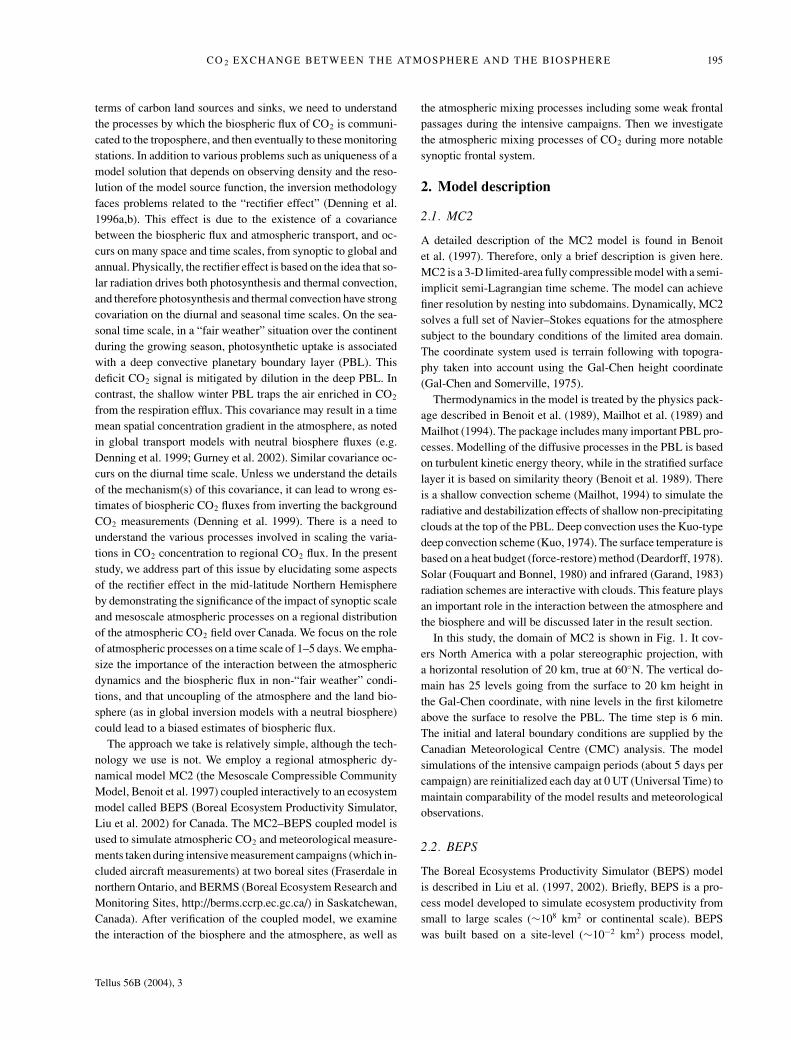
In this study, the domain of MC2 is shown in Fig. 1. It cov-ers North America with a polar stereographic projection, witha horizontal resolution of 20 km, true at 60◦N. The vertical do-main has 25 levels going from the surface to 20 km height inthe Gal-Chen coordinate, with nine levels in the first kilometreabove the surface to resolve the PBL. The time step is 6 min.The initial and lateral boundary conditions are supplied by theCanadian Meteorological Centre (CMC) analysis. The modelsimulations of the intensive campaign periods (about 5 days percampaign) are reinitialized each day at 0 UT (Universal Time) tomaintain comparability of the model results and meteorologicalobservations.

2.2. BEPS

The Boreal Ecosystems Productivity Simulator (BEPS) modelis described in Liu et al. (1997, 2002). Briefly, BEPS is a pro-cess model developed to simulate ecosystem productivity fromsmall to large scales (∼108 km2 or continental scale). BEPSwas built based on a site-level (∼10−2 km2) process model,

Tellus 56B (2004), 3

196 D. CHAN ET AL.

Fig 1. Map of the model domain of MC2. Also shown are the locationsof the Fraserdale and BERMS measurement sites, as well as thelocations of the three vertical cross-sections of the model resultsdiscussed in Section 3. The direction of the arrow indicates the left toright orientation in the vertical cross-section plots.

FOREST-BGC (Running and Coughlan, 1988). Scaling from siteto region was achieved through incorporating spatial data fromvarious sources. The data include leaf area index (LAI) derivedfrom advanced very high resolution radiometer (AVHRR) satel-lite measurements (Chen and Cihlar, 1996; Cihlar et al. 1997),land cover map data compatible with AVHRR (Cihlar et al. 1999)and the GIS soil database (Shields et al. 1991). The temporal in-terval is 10 to 11 days for LAI during the growing season. Theland cover map and soil data are both variant spatially but in-variant temporally in 1 year.

Significant modifications of BEPS from FOREST-BGC in-clude the canopy radiation calculation (Liu et al. 1997) andcanopy photosynthesis calculation (Liu et al. 2002). The rateof photosynthesis is critically dependent on the amount photo-synthetic active radiation (PAR) absorbed by the canopy. BEPStakes into account the fraction of PAR (FPAR) absorbed by thecanopy following the methods established by Chen (1996a,b).The absorbed PAR is separated into sunlit and shaded leaves andthe photosynthesis is calculated separately for these two groupsof leaves by the within-canopy spatial scaling scheme (Liu et al.2002).

With the meteorological forcing that includes shortwave ra-diation, temperature, humidity and precipitation, as well as veg-etation and soil data, BEPS computes net primary productivity(NPP), net ecosystem productivity (NEP), transpiration, evap-otranspiration, soil water content and other variables that char-acterize the ecosystem–atmosphere exchange. For the presentstudy the domain of BEPS is Canada. The coordinate system

used is the Lambert conformal conic projection with a resolu-tion of 1 km.

2.3. Coupled model

In this study, the two models, MC2 and BEPS, were coupledtogether. The coupling permitted examination and analyses ofthe exchange and interaction between the biosphere and the at-mosphere. There were some technical issues in the couplingexercise. The domain of MC2 uses the polar stereographic mapprojection with a horizontal resolution of 20 km and a time stepof 6 min, while BEPS employs the Lambert conformal conicprojection with a horizontal resolution of 1 km and a time stepof 1 h.

To achieve coupling, the two models were modified. A tracerequation with advection, diffusion and surface source terms wasadded to MC2 to model the atmospheric CO2 field. BEPS wasmodified from a daily time step to an hourly time step. The pro-cedure of coupling was as follows. First, the MC2 model wasexecuted to generate the hourly meteorological fields of surfacesolar radiation, temperature, humidity and precipitation. TheseMC2 outputs were then converted from the polar stereographicto the Lambert conformal conic projection and bilinearly inter-polated to the higher horizontal resolution of BEPS. BEPS wasthen driven with the MC2 meteorological outputs to yield hourlyNEP over Canada at a resolution of 1 km. The high-resolutionoutputs of BEPS were then summed and remapped to yield NEPover Canada on the 20 km resolution polar stereographic domainof MC2. Outside Canada, NEP was set to nil. The hourly BEPSNEP fluxes were interpolated onto the 6 min time step of MC2.Finally, MC2 was run again with the NEP surface fluxes to sim-ulate atmospheric evolution of the CO2 tracer. In this study, theanthropogenic and oceanic CO2 fluxes were not included.

The CO2 field in MC2 was initialized with a uniform con-centration (0 parts per million (ppm)). The initial concentrationserved as a reference for the time evolution of the CO2 field.Thus 0 ppm in the model corresponded to the mean backgroundtropospheric CO2 concentration (approximated by the CO2 con-centration from Alert (82◦27′ N, 62◦31′ W), Canada), which isabout 355 ppm in the observations for the July 2000 campaignat Fraserdale and about 360 ppm for the July 2002 campaign atBERMS. The CO2 field at the MC2 model boundary was fixedat 0 ppm. Since the MC2 model was reinitialized with CMCanalysis following each 1-day simulation, the CO2 field in MC2was saved at the end of each 1-day simulation and used as theinitial field for the following 1-day simulation. With the modelhorizontal resolution of 20 km, we will limit the discussion tothe synoptic and mesoscale processes resolvable in the model.

3. Model results and discussion

With a brief description of the regional atmospheric model(MC2) and the biospheric flux model (BEPS) completed, we

Tellus 56B (2004), 3

CO 2 EXCHANGE BETWEEN THE ATMOSPHERE AND THE BIOSPHERE 197

now focus on the verification and validation of the coupled modeland its ability to simulate the exchange processes between thebiosphere and the atmosphere.

With the exception of the years 1997, 1998 and parts of 1999,continuous measurements of atmospheric CO2 and meteorolog-ical conditions have been made since 1990 on a 40 m towerat Fraserdale (50◦N, 81◦W), located in a boreal forest site innorthern Ontario, Canada (Higuchi et al. 2003). The surround-ing ecosystem is dominated mainly by black spruce, followed bypoplar, jack pine and birch trees. During the period 1998–2000,the regular surface measurements were supplemented with sixintensive field campaigns, mostly during the growing season.

In 2002, to supplement the existing CO2 flux measurementprogramme at the BERMS site in Prince Albert, Saskatchewan,Canada (54◦N, 105◦W), we initiated the measurement of contin-uous CO2 concentration on the eddy-covariance CO2 flux towerat the old black spruce (OBS) location. One intensive aircraftcampaign in July 2002 was performed over the BERMS site.The locations of Fraserdale and BERMS are shown in Fig. 1.

On average, each campaign lasted for about 4–5 days, andconsisted of surface flask samples for isotopic analyses (as wellas for other trace gases) and vertical aircraft profiling that in-cluded in situ CO2 and meteorological measurements, as well asflask samples for trace gases and CO2 isotopes.

For the purpose of this study, we used the data gathered duringthe last two campaigns. These campaigns have the most completedata coverage and covered the effects of changing air masses.One campaign was at Fraserdale for the period of 25–29 July2000 (corresponding to the Julian days 207 to 211), and thesecond campaign was at BERMS for the period of 8–12 July2002 (corresponding to the Julian days 189 to 193). The coupledmodel was evaluated by comparing the model simulation with the

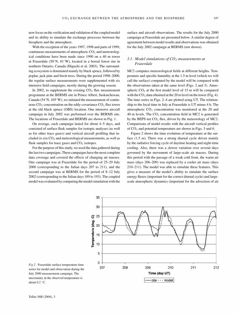
Fig 2. Fraserdale surface temperature timeseries for model and observation during theJuly 2000 measurement campaign. Theuncertainty in the observed temperature isabout 0.2 ◦C.

surface and aircraft observations. The results for the July 2000campaign at Fraserdale are presented below. A similar degree ofagreement between model results and observations was obtainedfor the July 2002 campaign at BERMS (not shown).

3.1. Model simulations of CO2 measurements atFraserdale

MC2 computes meteorological fields at different heights. Tem-perature and specific humidity at the 1.5 m level (which we willcall the surface) computed by the model will be compared withthe observations taken at the same level (Figs. 2 and 3). Atmo-spheric CO2 at the first model level of 15 m will be comparedwith the CO2 data obtained at the 20 m level on the tower (Fig. 4).The time series in Figs. 2–4 are plotted using UT. The relation-ship to the local time in July at Fraserdale is UT minus 4 h. Theatmospheric CO2 concentration was monitored at the 20 and40 m levels. The CO2 concentration field in MC2 is generatedby the BEPS net CO2 flux, driven by the meteorology of MC2.Comparisons of model results with the aircraft vertical profilesof CO2 and potential temperature are shown in Figs. 5 and 6.

Figure 2 shows the time evolution of temperature at the sur-face (1.5 m). There was a strong diurnal cycle driven mainlyby the radiative forcing cycle of daytime heating and night-timecooling. Also, there was a slower variation over several daysgoverned by the movement of large-scale air masses. Duringthis period with the passage of a weak cold front, the warm airmass (days 206–209) was replaced by a cooler air mass (days210–211). The model was able to simulate these features. Thisgives a measure of the model’s ability to simulate the surfaceenergy fluxes (important for the correct diurnal cycle) and large-scale atmospheric dynamics (important for the advection of air

Tellus 56B (2004), 3

198 D. CHAN ET AL.

Fig 3. Fraserdale model and observedsurface specific humidity q (g kg−1) timeseries for the July 2000 campaign. Theuncertainty in the observed specific humidityis about 0.2 g kg−1.

Fig 4. Fraserdale CO2 concentration (inppm) time series for the July 2000 campaign.Model results are for the 15 m level,measurements from the 20m level. Theuncertainty in the tower-observed CO2

concentration is about 0.1 ppm.

masses). There is general agreement between the model resultsand observations. The observed temperature record shows moreshort time scale variability than the model results, reflecting theexistence of small-scale processes not captured by the modelwith horizontal resolution of 20 km.

Figure 3 shows the surface specific humidity at the 1.5 mlevel. Model results and observations are in general agreement,though the model results are 1–2 g kg−1 drier. There are fewerdiurnal features in this field. As was the case with the surfacetemperature, the model does not capture all the short time scalevariability present in the observation. The model does, however,show the build-up of surface moisture before the passage ofthe weak cold front on day 209 and the reduction of surfacemoisture after the passage. The arrival of the drier air after the

passage of the weak cold front over Fraserdale was at ∼0 UT,day 210.

Figure 4 shows the CO2 concentration of the model at 15 mand the observation at 20 m. Both model results and observa-tions showed strong diurnal cycles in the CO2 concentration.The model results also compared well with the day to day vari-ability of the diurnal cycle (particularly before the passage of theweak cold front). The day to day variability of the diurnal cycleis a strong function of the characteristics (strength and thickness)of the night-time stable layer. Typically, a stable layer formedby radiative cooling will trap the night-time respired CO2 nearthe surface and build up a large night-time peak in the CO2 con-centration. The peak collapses in the morning with the onsetof photosynthetic draw-down and the breakdown of the surface

Tellus 56B (2004), 3

CO 2 EXCHANGE BETWEEN THE ATMOSPHERE AND THE BIOSPHERE 199

Fig 5. Vertical profiles of the model and observed CO2 (a) and potential temperature θ (b) for the afternoon of day 208 at Fraserdale (observationfrom an ascending profile). The uncertainty in the CO2 concentration is about 0.3 ppm, and about 0.2 K for potential temperature.

inversion layer. Different intensities of radiative cooling and sub-sidence will result in strong inversion in a shallow layer with acorresponding large nocturnal CO2 maximum, or weaker inver-sion in a deeper layer with a smaller nocturnal CO2 maximum.These processes are evident in the model (Stull, 1993; Bakwinet al. 1995, 1998).

The model results compared well with the observations fromday 206 to day 209. After the passage of the weak cold front, thedifference between model results and observations became large,especially on day 211. A possible factor affecting the model re-sults was the strong radiative cooling in the cool clear nights.Fraserdale cooled to ∼7 ◦C on day 211, compared with ∼15 ◦Con day 209. Since MC2 has only two levels in the lowest 100 m(15 m and 60 m), the shallow surface layer was not sufficientlywell resolved to yield the observed strong CO2 maximum. Thehighly stable surface layer was also evident in the observed CO2

concentration. There was a strong gradient in the CO2 concen-tration between the 20 and 40 m levels (not shown). Also, thenear-surface wind speed generally decreases at night (to as slowas 2 m s−1). With the weak wind, the observed CO2 at the towermay be strongly influenced by local variations in microscaletransport and biospheric flux variations. Heterogeneity near thetower, including a large reservoir, river valley and hills, may in-

fluence the measurements. Such small-scale processes are notsimulated in the model.

Aircraft measurements at Fraserdale consist of morning andafternoon vertical profiles to a 3 km height of continuous CO2

concentrations and meteorological data, as well as flask samplescollected for CO2 isotopes and other trace gases. Here we fo-cus on the change in the vertical structures of CO2 and potentialtemperature following the passage of a weak cold front. Figure 5shows the afternoon (20 UT, or 16 h local time) vertical pro-files of CO2 concentration (Fig. 5a) and potential temperature(Fig. 5b) for day 208, when Fraserdale was in the warm air mass.The afternoon well-mixed layer reached a height of ∼820 mb.Figure 6 shows the vertical profiles of CO2 concentration and po-tential temperature for day 210 at 20 UT (16 h local time), whenFraserdale was in the cool air mass. The afternoon well-mixedlayer reached only about 900 mb, although solar forcing, andthus surface heating, was greater on day 210 when Fraserdalewas in the clear cool air.

These results show that atmospheric dynamics of the differentair masses play an important role in the boundary layer dynamics.The strong stability of the subsiding cool air can cap the devel-opment of a well-mixed layer, while the large-scale lifting (orweaker subsidence) of the warm sector air, generally with some

Tellus 56B (2004), 3

200 D. CHAN ET AL.

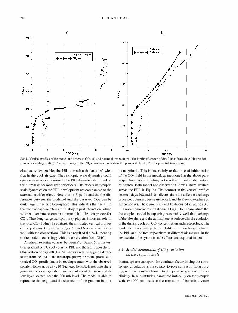
Fig 6. Vertical profiles of the model and observed CO2 (a) and potential temperature θ (b) for the afternoon of day 210 at Fraserdale (observationfrom an ascending profile). The uncertainty in the CO2 concentration is about 0.3 ppm, and about 0.2 K for potential temperature.

cloud activities, enables the PBL to reach a thickness of twicethat in the cool air case. Thus synoptic scale dynamics couldoperate in an opposite sense to the PBL dynamics described bythe diurnal or seasonal rectifier effects. The effects of synopticscale dynamics on the PBL development are comparable to theseasonal rectifier effect. Note that in Figs. 5a and 6a, the dif-ferences between the modelled and the observed CO2 can bequite large in the free troposphere. This indicates that the air inthe free troposphere retains the history of past interaction, whichwas not taken into account in our model initialization process forCO2. Thus long-range transport may play an important role inthe local CO2 budget. In contrast, the simulated vertical profilesof the potential temperature (Figs. 5b and 6b) agree relativelywell with the observations. This is a result of the 24-h updatingof the model meteorology with the observation from CMC.

Another interesting contrast between Figs. 5a and 6a is the ver-tical gradient of CO2 between the PBL and the free troposphere.Observation on day 208 (Fig. 5a) shows a relatively gradual tran-sition from the PBL to the free troposphere; the model produces avertical CO2 profile that is in good agreement with the observedprofile. However, on day 210 (Fig. 6a), the PBL-free tropospheregradient shows a large sharp increase of about 8 ppm in a shal-low layer located near the 900 mb level. The model is able toreproduce the height and the sharpness of the gradient but not

its magnitude. This is due mainly to the issue of initializationof the CO2 field in the model, as mentioned in the above para-graph. Another contributing factor is the limited model verticalresolution. Both model and observation show a sharp gradientacross the PBL in Fig. 6a. The contrast in the vertical profilesbetween days 208 and 210 indicates there are different exchangeprocesses operating between the PBL and the free troposphere ondifferent days. These processes will be discussed in Section 3.3.

The comparative results shown in Figs. 2 to 6 demonstrate thatthe coupled model is capturing reasonably well the exchangeof the biosphere and the atmosphere as reflected in the evolutionof the diurnal cycles of CO2 concentration and meteorology. Themodel is also capturing the variability of the exchange betweenthe PBL and the free troposphere in different air masses. In thenext section, the synoptic scale effects are explored in detail.

3.2. Model simulations of CO2 variationon the synoptic scale

In atmospheric transport, the dominant factor driving the atmo-spheric circulation is the equator-to-pole contrast in solar forc-ing, with the resultant horizontal temperature gradient or baro-clinicity. In mid-latitudes, baroclinic instability on the synopticscale (∼1000 km) leads to the formation of baroclinic waves

Tellus 56B (2004), 3

CO 2 EXCHANGE BETWEEN THE ATMOSPHERE AND THE BIOSPHERE 201

and frontal systems. In this subsection, we examine the effectsof these synoptic frontal systems on the coupling of biosphericCO2 flux and atmospheric transport. A typical case of a synopticevent has a horizontal potential temperature gradient �θ ∼ 10K, with a horizontal length scale �x ∼ 1000 km and a time scale�t ∼ 10 days.

The following sections will present a few cases of synopticsystems to illustrate a typical picture (showing the similarityand the ubiquity of the features) of the atmosphere–biosphereinteraction, as well as the differences between the cases.

3.2.1. Weak cold frontal passage at Fraserdale. During theJuly 2000 campaign, there was a passage of a weak cold fronton day 209 at Fraserdale (at ∼20 h local time or 0 UT, day210). With a demonstrated ability of the model to simulate theCO2 evolution during this period, our first case study of theatmospheric distribution of CO2 introduced into the PBL bythe BEPS biospheric flux was this cold front. Figure 1 showsthree 800 km long lines indicating the locations of the verticalcross-sections that will be discussed in this and the followingsections. The first cross-section (line 1) runs from James Bay toLake Huron, with Fraserdale located at the 200 km point on thedistance scale in the cross-section.

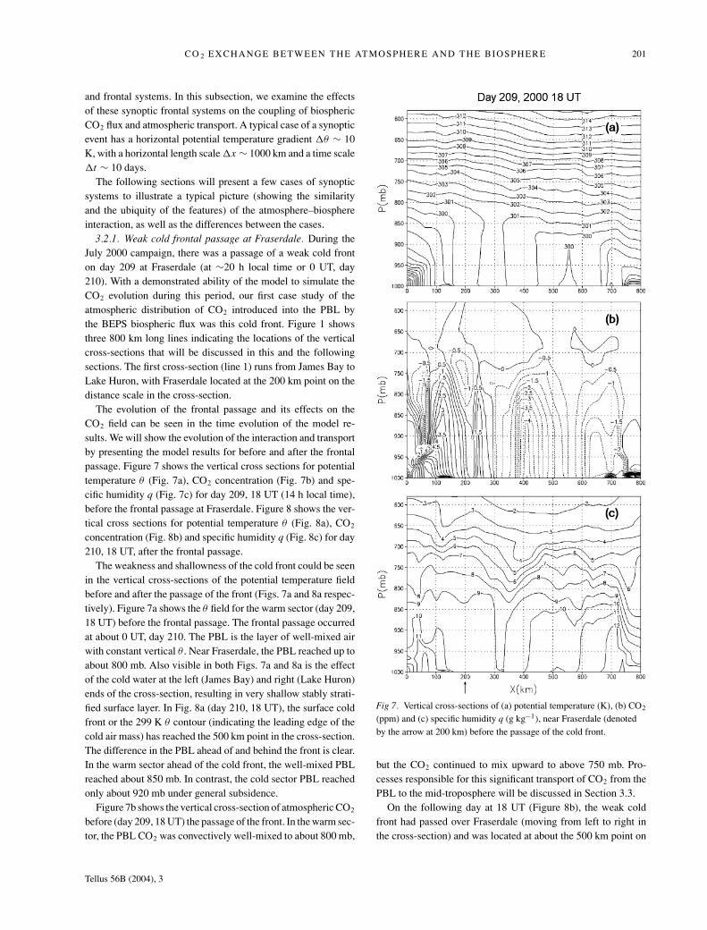
The evolution of the frontal passage and its effects on theCO2 field can be seen in the time evolution of the model re-sults. We will show the evolution of the interaction and transportby presenting the model results for before and after the frontalpassage. Figure 7 shows the vertical cross sections for potentialtemperature θ (Fig. 7a), CO2 concentration (Fig. 7b) and spe-cific humidity q (Fig. 7c) for day 209, 18 UT (14 h local time),before the frontal passage at Fraserdale. Figure 8 shows the ver-tical cross sections for potential temperature θ (Fig. 8a), CO2

concentration (Fig. 8b) and specific humidity q (Fig. 8c) for day210, 18 UT, after the frontal passage.

The weakness and shallowness of the cold front could be seenin the vertical cross-sections of the potential temperature fieldbefore and after the passage of the front (Figs. 7a and 8a respec-tively). Figure 7a shows the θ field for the warm sector (day 209,18 UT) before the frontal passage. The frontal passage occurredat about 0 UT, day 210. The PBL is the layer of well-mixed airwith constant vertical θ . Near Fraserdale, the PBL reached up toabout 800 mb. Also visible in both Figs. 7a and 8a is the effectof the cold water at the left (James Bay) and right (Lake Huron)ends of the cross-section, resulting in very shallow stably strati-fied surface layer. In Fig. 8a (day 210, 18 UT), the surface coldfront or the 299 K θ contour (indicating the leading edge of thecold air mass) has reached the 500 km point in the cross-section.The difference in the PBL ahead of and behind the front is clear.In the warm sector ahead of the cold front, the well-mixed PBLreached about 850 mb. In contrast, the cold sector PBL reachedonly about 920 mb under general subsidence.

Figure 7b shows the vertical cross-section of atmospheric CO2

before (day 209, 18 UT) the passage of the front. In the warm sec-tor, the PBL CO2 was convectively well-mixed to about 800 mb,

Fig 7. Vertical cross-sections of (a) potential temperature (K), (b) CO2

(ppm) and (c) specific humidity q (g kg−1), near Fraserdale (denotedby the arrow at 200 km) before the passage of the cold front.

but the CO2 continued to mix upward to above 750 mb. Pro-cesses responsible for this significant transport of CO2 from thePBL to the mid-troposphere will be discussed in Section 3.3.

On the following day at 18 UT (Figure 8b), the weak coldfront had passed over Fraserdale (moving from left to right inthe cross-section) and was located at about the 500 km point on

Tellus 56B (2004), 3

202 D. CHAN ET AL.

Fig 8. Vertical cross-sections of (a) potential temperature (K), (b) CO2

(ppm) and (c) specific humidity q (g kg−1), near Fraserdale (denotedby the arrow at 200 km) after the passage of the cold front.

the distance scale in the cross-section. The cold front pushes thewarm air ahead of it and forces it to rise above the cold air alongthe frontal surface. If there is sufficient moisture in the air, thenthe rising air condenses. This has two effects:

(1) Diabatic heating from condensation enhances the upwardflow of CO2 along the cold front. Sometimes, the heating pro-

duces enough buoyancy to overcome the stable stratificationleading to enhanced vertical transport.

(2) Clouds associated with the diabatic heating reduce solarradiation at the surface and consequently reduce photosynthesis.This leads to higher concentration of CO2 under the frontal cloudband.

These effects are visible as a cold frontal band of air withhigher CO2 concentration reaching up to about 700 mb. The firsteffect due to diabatic heating is visible as the band of air withhigh CO2 concentration rising along the sloping front to about900 mb, then almost vertically to about 700 mb.

Ahead of the cold front (right side of the 500 km mark inFig. 8b), the warm sector continued to exhibit deeply mixedPBL. In contrast, in the cold sector behind the front the PBL withwell-mixed CO2 reached only up to about 900 mb and is sharplycapped by strong vertical CO2 gradient. This is consistent withthe frontal features shown in the θ cross-section.

Besides the frontal features, these figures also show that thereare significant mesoscale features. In the warm sector, Fig. 7bshows horizontal variations in the CO2 concentration in the PBLof the order of 5 ppm per 100 km. The dynamics of these featureswill be discussed in Section 3.3.

The transition from the warm air to the cold air is also visiblein the time sequence of vertical cross-sections of the specifichumidity field shown in Figs. 7c and 8c for before and afterthe frontal passage, respectively. Figure 7c shows the q fieldwith little synoptic-scale gradient indicating that the cold fronthas not entered into the cross-section, while Fig. 8c shows asignificant gradient across the cold front, with drier air in thecold sector. Both figures show noticeable mesoscale featuresin the warm sector. These mesoscale features extend from thePBL into the free troposphere. In contrast, the cold sector PBLair is confined within the PBL (Fig. 8c). These features showthat the atmospheric transport processes are similar for the CO2

and q fields. The mesoscale dynamics of these features will bediscussed in Section 3.3.

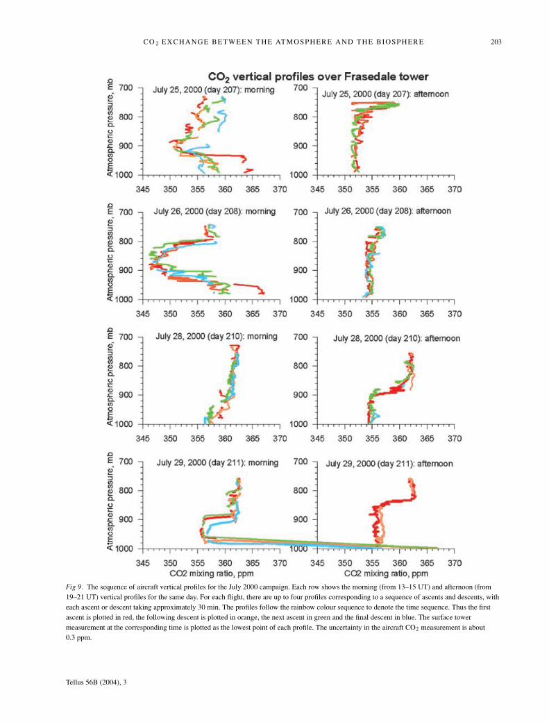
These results are qualitatively comparable to the campaignaircraft profiles of CO2 concentrations at Fraserdale shown inFig. 9. Each row in the figure shows the morning (from 13–15UT) and afternoon (from 19–21 UT) vertical profiles for the sameday. For each flight, there are up to four profiles corresponding toa sequence of ascents and descents, with each ascent or descenttaking approximately 30 min. The profiles follow the rainbowcolour order to denote the time sequence. Thus the first ascentis plotted in red, the following descent is plotted in orange, thenext ascent in green and the final descent in blue. The CO2 con-centration from the tower measurement is plotted as the lowestpoint of each profile. The observations were not taken on 27 July(day 209), the day of the frontal passage. However, as noted inSection 3.1, the sequence of the profiles shows the shallow PBLin the cold sector with large gradients across the PBL-free tropo-sphere boundary (the afternoon profiles on 28 July (day 210)),

Tellus 56B (2004), 3

CO 2 EXCHANGE BETWEEN THE ATMOSPHERE AND THE BIOSPHERE 203

Fig 9. The sequence of aircraft vertical profiles for the July 2000 campaign. Each row shows the morning (from 13–15 UT) and afternoon (from19–21 UT) vertical profiles for the same day. For each flight, there are up to four profiles corresponding to a sequence of ascents and descents, witheach ascent or descent taking approximately 30 min. The profiles follow the rainbow colour sequence to denote the time sequence. Thus the firstascent is plotted in red, the following descent is plotted in orange, the next ascent in green and the final descent in blue. The surface towermeasurement at the corresponding time is plotted as the lowest point of each profile. The uncertainty in the aircraft CO2 measurement is about0.3 ppm.

Tellus 56B (2004), 3

204 D. CHAN ET AL.

in contrast to the deep warm sector PBL with small transitionalgradients (the afternoon profiles on 26 July (day 208)). Withinthe warm sector, the sequence of morning profiles on 25 July(day 207) showed the advection of air with a higher CO2 con-centration to Fraserdale above the 900 mb level. For a typicalwind speed of 10 m s−1, the profiles capture the movement ofair with a CO2 gradient of about 5 ppm per 100 km. By com-paring the 25 July (day 207) afternoon profiles with the 26 July(day 208) morning profiles, there is evidence of an overnightadvection of air with a CO2 concentration about 5 ppm lower inthe PBL residual layer (between 900–800 mb). These mesoscalevariations of CO2 are comparable to the mesoscale variationssimulated in the model (see Figs. 7b and 8b).

There are prominent surface maxima in the CO2 profiles onthe morning of 29 July (day 211). On that morning, fog formedin the stable surface layer produced by the strong overnight ra-diative cooling. The ground fog delayed the surface warming inthe morning and the destruction of the stable night-time surfacelayer. Also, the fog reduced the surface solar radiation and pho-tosynthetic draw-down. Thus the large build-up of night-timerespired CO2 in the stable surface layer remained visible as thelarge surface CO2 maxima in the figure. The surface CO2 values(from the tower data) for the profiles were about 400 ppm.

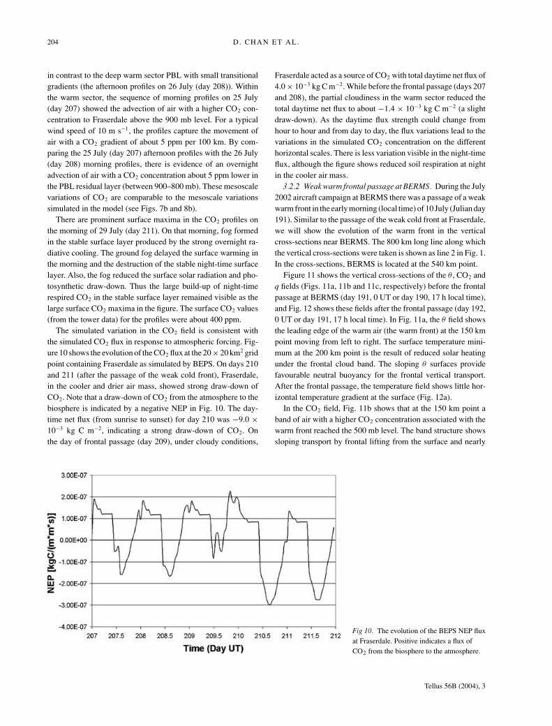
The simulated variation in the CO2 field is consistent withthe simulated CO2 flux in response to atmospheric forcing. Fig-ure 10 shows the evolution of the CO2 flux at the 20 × 20 km2 gridpoint containing Fraserdale as simulated by BEPS. On days 210and 211 (after the passage of the weak cold front), Fraserdale,in the cooler and drier air mass, showed strong draw-down ofCO2. Note that a draw-down of CO2 from the atmosphere to thebiosphere is indicated by a negative NEP in Fig. 10. The day-time net flux (from sunrise to sunset) for day 210 was −9.0 ×10−3 kg C m−2, indicating a strong draw-down of CO2. Onthe day of frontal passage (day 209), under cloudy conditions,

Fig 10. The evolution of the BEPS NEP fluxat Fraserdale. Positive indicates a flux ofCO2 from the biosphere to the atmosphere.

Fraserdale acted as a source of CO2 with total daytime net flux of4.0 × 10−3 kg C m−2. While before the frontal passage (days 207and 208), the partial cloudiness in the warm sector reduced thetotal daytime net flux to about −1.4 × 10−3 kg C m−2 (a slightdraw-down). As the daytime flux strength could change fromhour to hour and from day to day, the flux variations lead to thevariations in the simulated CO2 concentration on the differenthorizontal scales. There is less variation visible in the night-timeflux, although the figure shows reduced soil respiration at nightin the cooler air mass.

3.2.2 Weak warm frontal passage at BERMS. During the July2002 aircraft campaign at BERMS there was a passage of a weakwarm front in the early morning (local time) of 10 July (Julian day191). Similar to the passage of the weak cold front at Fraserdale,we will show the evolution of the warm front in the verticalcross-sections near BERMS. The 800 km long line along whichthe vertical cross-sections were taken is shown as line 2 in Fig. 1.In the cross-sections, BERMS is located at the 540 km point.

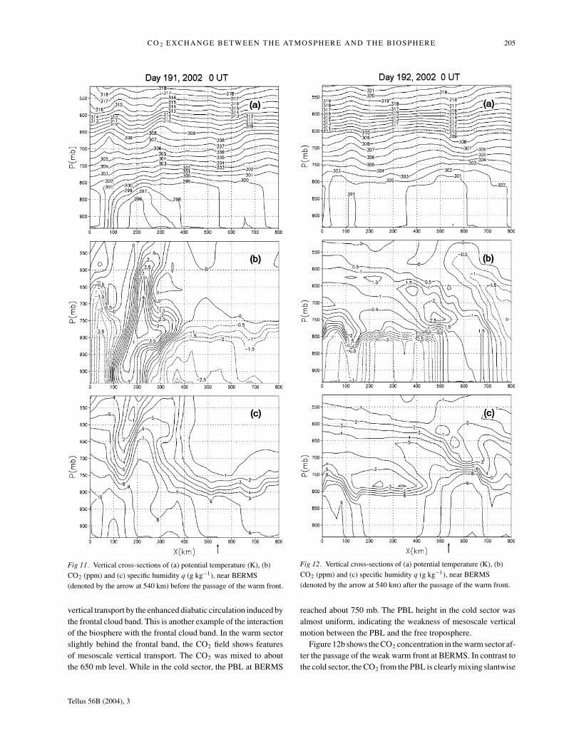
Figure 11 shows the vertical cross-sections of the θ , CO2 andq fields (Figs. 11a, 11b and 11c, respectively) before the frontalpassage at BERMS (day 191, 0 UT or day 190, 17 h local time),and Fig. 12 shows these fields after the frontal passage (day 192,0 UT or day 191, 17 h local time). In Fig. 11a, the θ field showsthe leading edge of the warm air (the warm front) at the 150 kmpoint moving from left to right. The surface temperature mini-mum at the 200 km point is the result of reduced solar heatingunder the frontal cloud band. The sloping θ surfaces providefavourable neutral buoyancy for the frontal vertical transport.After the frontal passage, the temperature field shows little hor-izontal temperature gradient at the surface (Fig. 12a).

In the CO2 field, Fig. 11b shows that at the 150 km point aband of air with a higher CO2 concentration associated with thewarm front reached the 500 mb level. The band structure showssloping transport by frontal lifting from the surface and nearly

Tellus 56B (2004), 3

CO 2 EXCHANGE BETWEEN THE ATMOSPHERE AND THE BIOSPHERE 205

Fig 11. Vertical cross-sections of (a) potential temperature (K), (b)CO2 (ppm) and (c) specific humidity q (g kg−1), near BERMS(denoted by the arrow at 540 km) before the passage of the warm front.

vertical transport by the enhanced diabatic circulation induced bythe frontal cloud band. This is another example of the interactionof the biosphere with the frontal cloud band. In the warm sectorslightly behind the frontal band, the CO2 field shows featuresof mesoscale vertical transport. The CO2 was mixed to aboutthe 650 mb level. While in the cold sector, the PBL at BERMS

Fig 12. Vertical cross-sections of (a) potential temperature (K), (b)CO2 (ppm) and (c) specific humidity q (g kg−1), near BERMS(denoted by the arrow at 540 km) after the passage of the warm front.

reached about 750 mb. The PBL height in the cold sector wasalmost uniform, indicating the weakness of mesoscale verticalmotion between the PBL and the free troposphere.

Figure 12b shows the CO2 concentration in the warm sector af-ter the passage of the weak warm front at BERMS. In contrast tothe cold sector, the CO2 from the PBL is clearly mixing slantwise

Tellus 56B (2004), 3

206 D. CHAN ET AL.

into the free troposphere near BERMS up to about the 600 mblevel. The strongly sloping transport coupled with the mesoscalevariations in the CO2 concentration result in the complex lay-ered structures in the free troposphere near BERMS. There is achange in the sloping transport compared with the warm front inFig. 11b. Clearly the upper airflow has shifted behind the front.As in the weak cold front simulation near Fraserdale, there aresignificant horizontal variations in CO2 concentrations of the or-der of 5–10 ppm over a distance of about 100 km. Also notablein Fig. 12b is the region from about 200 km to 500 km, wherethe CO2 in the PBL appears capped at the top of the PBL. Thislack of mixing above the PBL is related to the moisture fieldpresented next.

In Figure 11c, the q field shows the horizontal gradient ofmoisture from the moist air in the warm sector to the drier air inthe cold sector. The vertical motion of the warm front and in thewarm sector above the PBL, and the lack of vertical mixing atthe top of the PBL in the cold sector, are both consistent with themodelled CO2 field in Fig. 11b. In Fig. 12c, after the passage ofthe weak warm front, the slantwise transport of humidity acrossthe PBL to the free troposphere is again evident near BERMS,similar to the CO2 field. The region from about 200 km to 500km has relatively low humidity. The drier air in this region is notfavourable for cloud formation and diabatically forced circula-tion. This result is evident from the lack of exchange between thePBL and the free troposphere. Since CO2 acts as a passive tracerin the atmosphere, this also explains the lack of vertical mixingof CO2 in this region noted previously. Similarly, the “dry” coldsectors in these examples have little exchange between the PBLand the free troposphere. These results indicate that CO2 mixingis strongly coupled to the mesoscale and synoptic scale transportand diabatic processes.

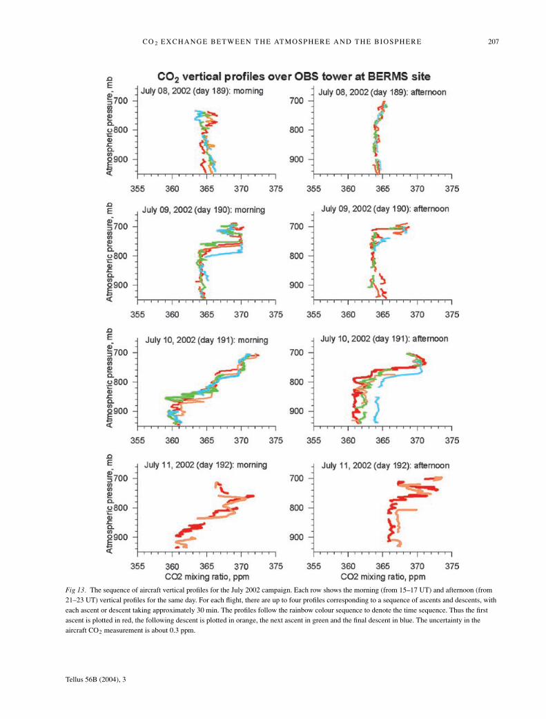
Again the model results can be compared qualitatively withthe campaign aircraft vertical profiles of CO2 concentrations atBERMS shown in Fig. 13. In Fig. 13, the surface tower CO2 dataare not plotted as the surface value of the profiles since the dataare not yet available. Although the sequence of vertical profilescontains a great deal of detail, it is possible to delineate certainprominent features. A comparison of the afternoon profiles on 9July (day 190, before the frontal passage) to the morning profileson 10 July (day 191, after the frontal passage) shows that the fronttransported air with a lower CO2 concentration below 850 mb andair with a higher CO2 concentration above 800 mb to BERMS.These changes in the CO2 concentrations of about 5 ppm arecomparable to the modelled CO2 variations near the front. Awayfrom the warm front, the 10 July (day 191) afternoon aircraftprofiles show the CO2 concentration in the whole PBL to beincreasing with time. This was the result of an advection of airin the warm sector with a horizontal CO2 gradient of about 4ppm over a distance of about 100 km (for a typical wind speedof 10 m s−1). Another example of advection in the warm sectoris the difference in the vertical profiles between the afternoonof 10 July (day 191) and the morning of 11 July (day 192). The

morning profiles indicate air with a lower CO2 concentrationbelow 850 mb, as well as above 750 mb, compared with theprevious afternoon profiles. These results are consistent withthe modelled CO2 field with horizontal mesoscale (∼100 km)variations and vertically complex layered structures above thePBL. The layered structures are again evident in the afternoonprofiles on 11 July (day 192).

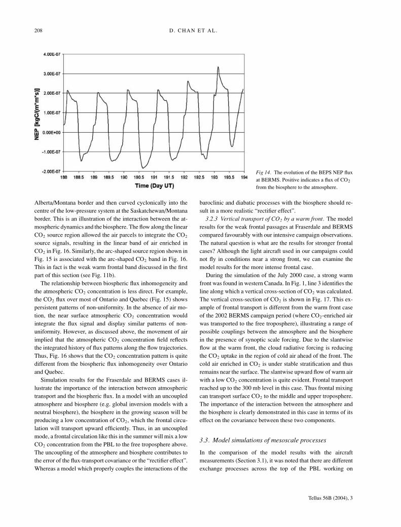
The evolution of the simulated CO2 flux at BERMS is pre-sented in Fig. 14. The response of the CO2 flux to the meteoro-logical forcing is again evident in the day to day variations ofthe total daytime net flux. With BERMS in the cooler air on day190, the total daytime net flux was −6.0 × 10−3 kg C m−2 (astrong draw-down of CO2). Then, in the warm air sector on day193, the BERMS area under cloudy condition became a CO2

source with a total daytime net flux of 2 × 10−3 kg C m−2. Thusthe subsynoptic scale (or mesoscale) variations in the CO2 fluxare comparable to the synoptic scale variations in the Fraserdalecase, Fig. 10.

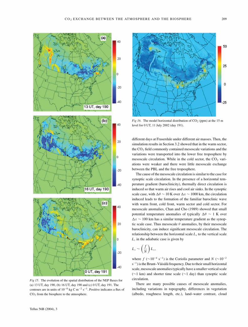
Figures 10 and 14 showed the local picture of the CO2 fluxvariations. It is also informative to show the temporal evolutionof the spatial distribution of the CO2 flux. Figures 15a , 15b and15c show the BEPS CO2 flux for 13 UT of day 190, 16 UT ofday 190 and 0 UT of day 191 respectively. At 13 UT, day 190 inFig. 15a, the CO2 flux distribution showed strong draw-down inmuch of Ontario and Quebec where the local time was 9 h. Whilein Alberta and Saskatchewan, the daytime draw-down was be-ginning where the local time was 7 h. However, there were twoprominent cloud bands which induced the two banded regionsof CO2 source fluxes, one arc shaped band in southern Albertaand Saskatchewan and one linear band from southern Albertato northern Alberta. These bands of CO2 source regions per-sisted for many hours and remained visible at 16 UT, day 190in Fig. 15b. The linear CO2 source region dissipated gradually(along with the cloud band) as the day progressed. In Fig. 15cat 0 UT, day 191, the linear band of CO2 source had vanishedand was replaced by a mixed pattern of sources and sinks. Thearc-shaped band of CO2 source in southern Saskatchewan per-sisted and showed propagation with time (with the movementof the cloud band). Also visible in southern Saskatchewan inFig. 15c were other band-shaped regions of CO2 sources andsinks. In general, the CO2 flux variations due to meteorologicalconditions are typically larger than the CO2 flux variations dueto the heterogeneity in the vegetation.

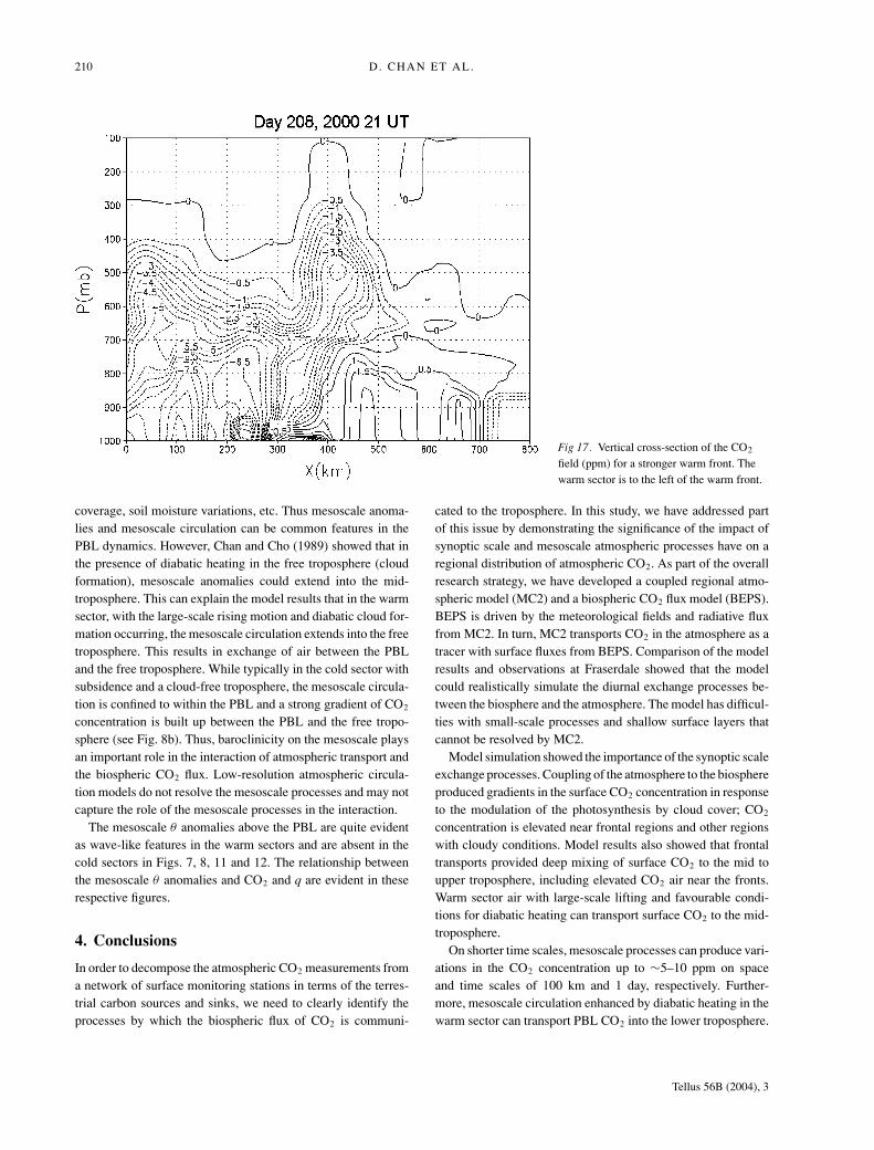
The atmospheric CO2 field contains the integrated history ofthe surface CO2 flux forcing. This relationship is quite evidentin the surface distribution of the atmospheric CO2 concentra-tion field for 0 UT, day 191, Fig. 16. There are banded fea-tures in the CO2 field in Alberta and Saskatchewan correspond-ing to the banded regions of CO2 source fluxes in Alberta andSaskatchewan (Fig. 15). Figure 15 showed that the linear-shapedCO2 source region did not extend to the Alberta/Montana border.However, the banded feature in the CO2 field showed that theair high in CO2 was transported from the source region to the

Tellus 56B (2004), 3

CO 2 EXCHANGE BETWEEN THE ATMOSPHERE AND THE BIOSPHERE 207

Fig 13. The sequence of aircraft vertical profiles for the July 2002 campaign. Each row shows the morning (from 15–17 UT) and afternoon (from21–23 UT) vertical profiles for the same day. For each flight, there are up to four profiles corresponding to a sequence of ascents and descents, witheach ascent or descent taking approximately 30 min. The profiles follow the rainbow colour sequence to denote the time sequence. Thus the firstascent is plotted in red, the following descent is plotted in orange, the next ascent in green and the final descent in blue. The uncertainty in theaircraft CO2 measurement is about 0.3 ppm.

Tellus 56B (2004), 3

208 D. CHAN ET AL.

Fig 14. The evolution of the BEPS NEP fluxat BERMS. Positive indicates a flux of CO2

from the biosphere to the atmosphere.

Alberta/Montana border and then curved cyclonically into thecentre of the low-pressure system at the Saskatchewan/Montanaborder. This is an illustration of the interaction between the at-mospheric dynamics and the biosphere. The flow along the linearCO2 source region allowed the air parcels to integrate the CO2

source signals, resulting in the linear band of air enriched inCO2 in Fig. 16. Similarly, the arc-shaped source region shown inFig. 15 is associated with the arc-shaped CO2 band in Fig. 16.This in fact is the weak warm frontal band discussed in the firstpart of this section (see Fig. 11b).

The relationship between biospheric flux inhomogeneity andthe atmospheric CO2 concentration is less direct. For example,the CO2 flux over most of Ontario and Quebec (Fig. 15) showspersistent patterns of non-uniformity. In the absence of air mo-tion, the near surface atmospheric CO2 concentration wouldintegrate the flux signal and display similar patterns of non-uniformity. However, as discussed above, the movement of airimplied that the atmospheric CO2 concentration field reflectsthe integrated history of flux patterns along the flow trajectories.Thus, Fig. 16 shows that the CO2 concentration pattern is quitedifferent from the biospheric flux inhomogeneity over Ontarioand Quebec.

Simulation results for the Fraserdale and BERMS cases il-lustrate the importance of the interaction between atmospherictransport and the biospheric flux. In a model with an uncoupledatmosphere and biosphere (e.g. global inversion models with aneutral biosphere), the biosphere in the growing season will beproducing a low concentration of CO2, which the frontal circu-lation will transport upward efficiently. Thus, in an uncoupledmode, a frontal circulation like this in the summer will mix a lowCO2 concentration from the PBL to the free troposphere above.The uncoupling of the atmosphere and biosphere contributes tothe error of the flux-transport covariance or the “rectifier effect”.Whereas a model which properly couples the interactions of the

baroclinic and diabatic processes with the biosphere should re-sult in a more realistic “rectifier effect”.

3.2.3 Vertical transport of CO2 by a warm front. The modelresults for the weak frontal passages at Fraserdale and BERMScompared favourably with our intensive campaign observations.The natural question is what are the results for stronger frontalcases? Although the light aircraft used in our campaigns couldnot fly in conditions near a strong front, we can examine themodel results for the more intense frontal case.

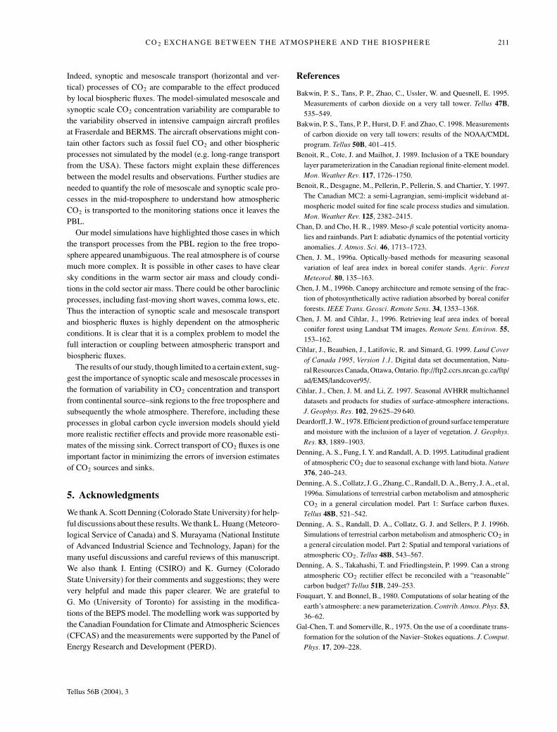
During the simulation of the July 2000 case, a strong warmfront was found in western Canada. In Fig. 1, line 3 identifies theline along which a vertical cross-section of CO2 was calculated.The vertical cross-section of CO2 is shown in Fig. 17. This ex-ample of frontal transport is different from the warm front caseof the 2002 BERMS campaign period (where CO2-enriched airwas transported to the free troposphere), illustrating a range ofpossible couplings between the atmosphere and the biospherein the presence of synoptic scale forcing. Due to the slantwiseflow at the warm front, the cloud radiative forcing is reducingthe CO2 uptake in the region of cold air ahead of the front. Thecold air enriched in CO2 is under stable stratification and thusremains near the surface. The slantwise upward flow of warm airwith a low CO2 concentration is quite evident. Frontal transportreached up to the 300 mb level in this case. Thus frontal mixingcan transport surface CO2 to the middle and upper troposphere.The importance of the interaction between the atmosphere andthe biosphere is clearly demonstrated in this case in terms of itseffect on the covariance between these two components.

3.3. Model simulations of mesoscale processes

In the comparison of the model results with the aircraftmeasurements (Section 3.1), it was noted that there are differentexchange processes across the top of the PBL working on

Tellus 56B (2004), 3

CO 2 EXCHANGE BETWEEN THE ATMOSPHERE AND THE BIOSPHERE 209

Fig 15. The evolution of the spatial distribution of the NEP fluxes for(a) 13 UT, day 190, (b) 16 UT, day 190 and (c) 0 UT, day 191. Thecontours are in units of 10−8 kg C m−2 s−1. Positive indicates a flux ofCO2 from the biosphere to the atmosphere.

Fig 16. The model horizontal distribution of CO2 (ppm) at the 15 mlevel for 0 UT, 11 July 2002 (day 191).

different days at Fraserdale under different air masses. Then, thesimulation results in Section 3.2 showed that in the warm sector,the CO2 field commonly contained mesoscale variations and thevariations were transported into the lower free troposphere bymesoscale circulation. While in the cold sector, the CO2 vari-ations were weaker and there were little mesoscale exchangebetween the PBL and the free troposphere.

The cause of the mesoscale circulation is similar to the case forsynoptic scale circulation. In the presence of a horizontal tem-perature gradient (baroclinicity), thermally direct circulation isinduced so that warm air rises and cool air sinks. In the synopticscale case, with �θ ∼ 10 K over �x ∼ 1000 km, the circulationinduced leads to the formation of the familiar baroclinic wavewith warm front, cold front, warm sector and cold sector. Formesoscale anomalies, Chan and Cho (1989) showed that smallpotential temperature anomalies of typically �θ ∼ 1 K over�x ∼ 100 km has a similar temperature gradient as the synop-tic scale case. Thus mesoscale θ anomalies, by their mesoscalebaroclinicity, can induce significant mesoscale circulation. Therelationship between the horizontal scale Lx to the vertical scaleLz in the adiabatic case is given by

Lz ∼(

f

N

)Lx ,

where f (∼10−4 s−1) is the Coriolis parameter and N (∼10−2

s−1) is the Brunt–Vaisala frequency. Due to their small horizontalscale, mesoscale anomalies typically have a smaller vertical scale(∼1 km) and shorter time scale (∼1 day) than synoptic scalecirculation.

There are many possible causes of mesoscale anomalies,including variations in topography, differences in vegetation(albedo, roughness length, etc.), land–water contrast, cloud

Tellus 56B (2004), 3

210 D. CHAN ET AL.

Fig 17. Vertical cross-section of the CO2

field (ppm) for a stronger warm front. Thewarm sector is to the left of the warm front.

coverage, soil moisture variations, etc. Thus mesoscale anoma-lies and mesoscale circulation can be common features in thePBL dynamics. However, Chan and Cho (1989) showed that inthe presence of diabatic heating in the free troposphere (cloudformation), mesoscale anomalies could extend into the mid-troposphere. This can explain the model results that in the warmsector, with the large-scale rising motion and diabatic cloud for-mation occurring, the mesoscale circulation extends into the freetroposphere. This results in exchange of air between the PBLand the free troposphere. While typically in the cold sector withsubsidence and a cloud-free troposphere, the mesoscale circula-tion is confined to within the PBL and a strong gradient of CO2

concentration is built up between the PBL and the free tropo-sphere (see Fig. 8b). Thus, baroclinicity on the mesoscale playsan important role in the interaction of atmospheric transport andthe biospheric CO2 flux. Low-resolution atmospheric circula-tion models do not resolve the mesoscale processes and may notcapture the role of the mesoscale processes in the interaction.

The mesoscale θ anomalies above the PBL are quite evidentas wave-like features in the warm sectors and are absent in thecold sectors in Figs. 7, 8, 11 and 12. The relationship betweenthe mesoscale θ anomalies and CO2 and q are evident in theserespective figures.

4. Conclusions

In order to decompose the atmospheric CO2 measurements froma network of surface monitoring stations in terms of the terres-trial carbon sources and sinks, we need to clearly identify theprocesses by which the biospheric flux of CO2 is communi-

cated to the troposphere. In this study, we have addressed partof this issue by demonstrating the significance of the impact ofsynoptic scale and mesoscale atmospheric processes have on aregional distribution of atmospheric CO2. As part of the overallresearch strategy, we have developed a coupled regional atmo-spheric model (MC2) and a biospheric CO2 flux model (BEPS).BEPS is driven by the meteorological fields and radiative fluxfrom MC2. In turn, MC2 transports CO2 in the atmosphere as atracer with surface fluxes from BEPS. Comparison of the modelresults and observations at Fraserdale showed that the modelcould realistically simulate the diurnal exchange processes be-tween the biosphere and the atmosphere. The model has difficul-ties with small-scale processes and shallow surface layers thatcannot be resolved by MC2.

Model simulation showed the importance of the synoptic scaleexchange processes. Coupling of the atmosphere to the biosphereproduced gradients in the surface CO2 concentration in responseto the modulation of the photosynthesis by cloud cover; CO2

concentration is elevated near frontal regions and other regionswith cloudy conditions. Model results also showed that frontaltransports provided deep mixing of surface CO2 to the mid toupper troposphere, including elevated CO2 air near the fronts.Warm sector air with large-scale lifting and favourable condi-tions for diabatic heating can transport surface CO2 to the mid-troposphere.

On shorter time scales, mesoscale processes can produce vari-ations in the CO2 concentration up to ∼5–10 ppm on spaceand time scales of 100 km and 1 day, respectively. Further-more, mesoscale circulation enhanced by diabatic heating in thewarm sector can transport PBL CO2 into the lower troposphere.

Tellus 56B (2004), 3

CO 2 EXCHANGE BETWEEN THE ATMOSPHERE AND THE BIOSPHERE 211

Indeed, synoptic and mesoscale transport (horizontal and ver-tical) processes of CO2 are comparable to the effect producedby local biospheric fluxes. The model-simulated mesoscale andsynoptic scale CO2 concentration variability are comparable tothe variability observed in intensive campaign aircraft profilesat Fraserdale and BERMS. The aircraft observations might con-tain other factors such as fossil fuel CO2 and other biosphericprocesses not simulated by the model (e.g. long-range transportfrom the USA). These factors might explain these differencesbetween the model results and observations. Further studies areneeded to quantify the role of mesoscale and synoptic scale pro-cesses in the mid-troposphere to understand how atmosphericCO2 is transported to the monitoring stations once it leaves thePBL.

Our model simulations have highlighted those cases in whichthe transport processes from the PBL region to the free tropo-sphere appeared unambiguous. The real atmosphere is of coursemuch more complex. It is possible in other cases to have clearsky conditions in the warm sector air mass and cloudy condi-tions in the cold sector air mass. There could be other baroclinicprocesses, including fast-moving short waves, comma lows, etc.Thus the interaction of synoptic scale and mesoscale transportand biospheric fluxes is highly dependent on the atmosphericconditions. It is clear that it is a complex problem to model thefull interaction or coupling between atmospheric transport andbiospheric fluxes.

The results of our study, though limited to a certain extent, sug-gest the importance of synoptic scale and mesoscale processes inthe formation of variability in CO2 concentration and transportfrom continental source–sink regions to the free troposphere andsubsequently the whole atmosphere. Therefore, including theseprocesses in global carbon cycle inversion models should yieldmore realistic rectifier effects and provide more reasonable esti-mates of the missing sink. Correct transport of CO2 fluxes is oneimportant factor in minimizing the errors of inversion estimatesof CO2 sources and sinks.

5. Acknowledgments

We thank A. Scott Denning (Colorado State University) for help-ful discussions about these results. We thank L. Huang (Meteoro-logical Service of Canada) and S. Murayama (National Instituteof Advanced Industrial Science and Technology, Japan) for themany useful discussions and careful reviews of this manuscript.We also thank I. Enting (CSIRO) and K. Gurney (ColoradoState University) for their comments and suggestions; they werevery helpful and made this paper clearer. We are grateful toG. Mo (University of Toronto) for assisting in the modifica-tions of the BEPS model. The modelling work was supported bythe Canadian Foundation for Climate and Atmospheric Sciences(CFCAS) and the measurements were supported by the Panel ofEnergy Research and Development (PERD).

References

Bakwin, P. S., Tans, P. P., Zhao, C., Ussler, W. and Quesnell, E. 1995.Measurements of carbon dioxide on a very tall tower. Tellus 47B,535–549.

Bakwin, P. S., Tans, P. P., Hurst, D. F. and Zhao, C. 1998. Measurementsof carbon dioxide on very tall towers: results of the NOAA/CMDLprogram. Tellus 50B, 401–415.

Benoit, R., Cote, J. and Mailhot, J. 1989. Inclusion of a TKE boundarylayer parameterization in the Canadian regional finite-element model.Mon. Weather Rev. 117, 1726–1750.

Benoit, R., Desgagne, M., Pellerin, P., Pellerin, S. and Chartier, Y. 1997.The Canadian MC2: a semi-Lagrangian, semi-implicit wideband at-mospheric model suited for fine scale process studies and simulation.Mon. Weather Rev. 125, 2382–2415.

Chan, D. and Cho, H. R., 1989. Meso-β scale potential vorticity anoma-lies and rainbands. Part I: adiabatic dynamics of the potential vorticityanomalies. J. Atmos. Sci. 46, 1713–1723.

Chen, J. M., 1996a. Optically-based methods for measuring seasonalvariation of leaf area index in boreal conifer stands. Agric. ForestMeteorol. 80, 135–163.

Chen, J. M., 1996b. Canopy architecture and remote sensing of the frac-tion of photosynthetically active radiation absorbed by boreal coniferforests. IEEE Trans. Geosci. Remote Sens. 34, 1353–1368.

Chen, J. M. and Cihlar, J., 1996. Retrieving leaf area index of borealconifer forest using Landsat TM images. Remote Sens. Environ. 55,153–162.

Cihlar, J., Beaubien, J., Latifovic, R. and Simard, G. 1999. Land Coverof Canada 1995, Version 1.1. Digital data set documentation, Natu-ral Resources Canada, Ottawa, Ontario. ftp://ftp2.ccrs.nrcan.gc.ca/ftp/ad/EMS/landcover95/.

Cihlar, J., Chen, J. M. and Li, Z. 1997. Seasonal AVHRR multichanneldatasets and products for studies of surface-atmosphere interactions.J. Geophys. Res. 102, 29 625–29 640.

Deardorff, J. W., 1978. Efficient prediction of ground surface temperatureand moisture with the inclusion of a layer of vegetation. J. Geophys.Res. 83, 1889–1903.

Denning, A. S., Fung, I. Y. and Randall, A. D. 1995. Latitudinal gradientof atmospheric CO2 due to seasonal exchange with land biota. Nature376, 240–243.

Denning, A. S., Collatz, J. G., Zhang, C., Randall, D. A., Berry, J. A., et al,1996a. Simulations of terrestrial carbon metabolism and atmosphericCO2 in a general circulation model. Part 1: Surface carbon fluxes.Tellus 48B, 521–542.

Denning, A. S., Randall, D. A., Collatz, G. J. and Sellers, P. J. 1996b.Simulations of terrestrial carbon metabolism and atmospheric CO2 ina general circulation model. Part 2: Spatial and temporal variations ofatmospheric CO2. Tellus 48B, 543–567.

Denning, A. S., Takahashi, T. and Friedlingstein, P. 1999. Can a strongatmospheric CO2 rectifier effect be reconciled with a “reasonable”carbon budget? Tellus 51B, 249–253.

Fouquart, Y. and Bonnel, B., 1980. Computations of solar heating of theearth’s atmosphere: a new parameterization. Contrib. Atmos. Phys. 53,36–62.

Gal-Chen, T. and Somerville, R., 1975. On the use of a coordinate trans-formation for the solution of the Navier–Stokes equations. J. Comput.Phys. 17, 209–228.

Tellus 56B (2004), 3

212 D. CHAN ET AL.

Garand, L., 1983. Some improvements and complements to the infraredemissivity algorithm including a parameterization of the absorptionin the continuum region. J. Atmos. Sci. 40, 230–244.

Gurney, R. K., Law, R. M., Denning, A. S., Rayner, P. J., Baker, D.,et al, 2002. Towards robust regional estimates of CO2 sourcesand sinks using atmospheric transport models. Nature 415, 626–630.

Higuchi, K., Worthy, D., Chan, D. and Shashkov, A. 2003. Regionalsource/sink impact on diurnal, seasonal and inter-annual variationsin atmospheric CO2 at a boreal forest site in Canada. Tellus 55B,115–125.

Kuo, H. L., 1974. Further studies of the parameterization of the influenceof cumulus convection on large-scale flow. J. Atmos. Sci. 46, 545–564.

Liu, J., Chen, J. M., Cihlar, J. and Park, W. M. 1997. A process-basedboreal ecosystem productivity simulator using remote sensing inputs.Remote Sens. Environ. 62, 158–175.

Liu, J., Chen, J.M., Cihlar, J. and Chen, W. 2002. Net primary produc-

tivity mapped for Canada at 1-km resolution, Global Ecol. Biogeog.11, 115–129.

Mailhot, J., 1994. The Regional Finite-element (RFE) Model Scien-tific Description. Part 2: Physics. (Available from RPN, 2121 Trans-Canada, Dorval, QC H9P 1J3, Canada.)

Mailhot, J., Chouinard, C., Benoit, R., Roch, M., Verner, G., Cote, J. andPudykiewicz, J. 1989. Numerical forecasting of winter coastal stormsduring CASP: evaluation of the regional finite-element model. Atmos.Ocean 27, 27–58.

Running, S. W. and Coughlan, J. C., 1988. A general model of the forestecosystem processes for regional applications I: hydrological balance,canopy gas exchange and primary production processes. Ecol. Model.42, 125–154.

Shields, J. A., Tarnocai, C., Valentine, K. W. G. and MacDonald, K. B.1991. Soil Landscapes of Canada: Procedures Manual and User′sHandbook. Agriculture Canada Publication 1868/E, Ottawa, Canada.

Stull, R. B., 1993. An Introduction to Boundary Layer Meteorology.Kluwer Academic Publishers, Dordrecht.

Tellus 56B (2004), 3