On the “bridge hill” of the violin - · PDF fileOn the “bridge hill”...

Bridge hill/Woodhouse 1 May 25, 2004

On the “bridge hill” of the violin

J. WoodhouseCambridge University Engineering Department,

Trumpington St, Cambridge CB2 1PZ, U.K.

[email protected]

Summary

Many excellent violins show a broad peak of response in the vicinity of 2.5 kHz, a featurewhich has been called the “bridge hill”. It is demonstrated using simplified theoretical modelsthat this feature arises from a combination of an in-plane resonance of the bridge and anaveraged version of the response of the violin body at the bridge-foot positions. Using atechnique from statistical vibration analysis, it is possible to extract the “skeleton” of thebridge hill in a very clear form. Parameter studies are then presented which reveal how thebridge hill is affected, in some cases with great sensitivity, by the properties of the bridge andbody. The results seem to account for behaviour seen in earlier experimental studies, and theyhave direct relevance to violin makers for guiding the adjustment of bridges to achieve desiredtonal quality.

PACS No. 43.75.De

1. Introduction

The characteristic high bridge of the violin and cello, and indeed of most bowed-stringinstruments, presumably developed initially for ergonomic reasons. In order to provide therange of angles needed to bow each string individually, the strings must be raised clear of theinstrument body. Also, the high bridge plays an essential role in “rotating” the transverseforce from the vibrating string into normal forces applied to the instrument body through thebridge feet, which can then excite bending vibration of the body [1]. Compared to the low,robust bridges of the piano or guitar, the violin bridge may seem to be a necessary evil: it isfragile and requires regular attention to keep it straight and properly fitted. However, researchof recent years shows that this type of bridge has provided, perhaps somewhat fortuitously, acrucial means for adjustment of the string-to-body impedance characteristics which hasallowed the violin family to acquire its familiar loudness and tonal colouration.

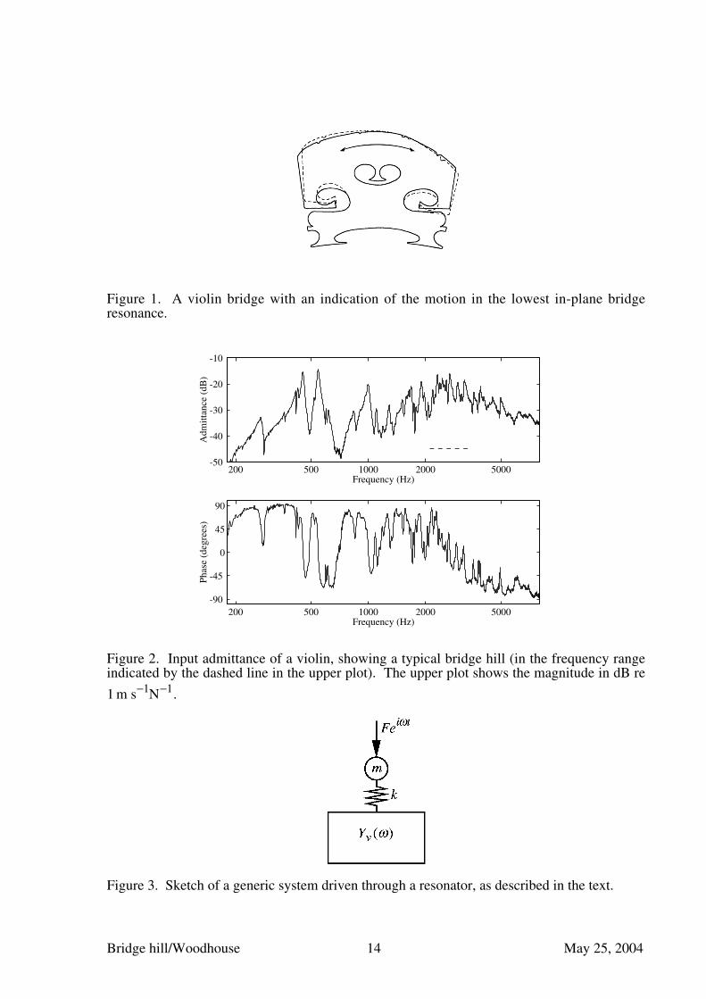
The oscillating force provided by the vibrating string can only excite vibration of theinstrument body by first passing through the bridge. The bridge thus acts as a filter, and it isno surprise that the material properties and geometric configuration of the bridge can have asignificant influence on the sound of an instrument. The first systematic study of thetransmission properties of the violin bridge was made by Reinicke and Cremer [1,2]. Theyshowed that a normal violin bridge has internal resonances within the frequency range ofinterest for the sound of the instrument, so that the filtering effect of the bridge has verysignificant variation with frequency. The lowest bridge resonance is usually found around3 kHz when the bridge feet are held rigidly (for example in a vice), and the motion consists ofside-to-side rocking of the top portion of the bridge as sketched in Fig. 1.

Since the work of Reinicke and Cremer, several experimental studies have been carried outwhich relate to the influence of this lowest bridge resonance. First, measurements have beenmade by Dünnwald [3] and Jansson [4,5] of the frequency response of a wide variety ofviolins. Both authors found that violins of high market value showed a strong tendency toexhibit a broad peak of response in the vicinity of 2–3 kHz, in a feature originally named the“bridge hill” by Jansson. The name was given because he, and indeed Cremer [1], attributedthis feature to the filtering effect of the lowest bridge resonance just described. A typical


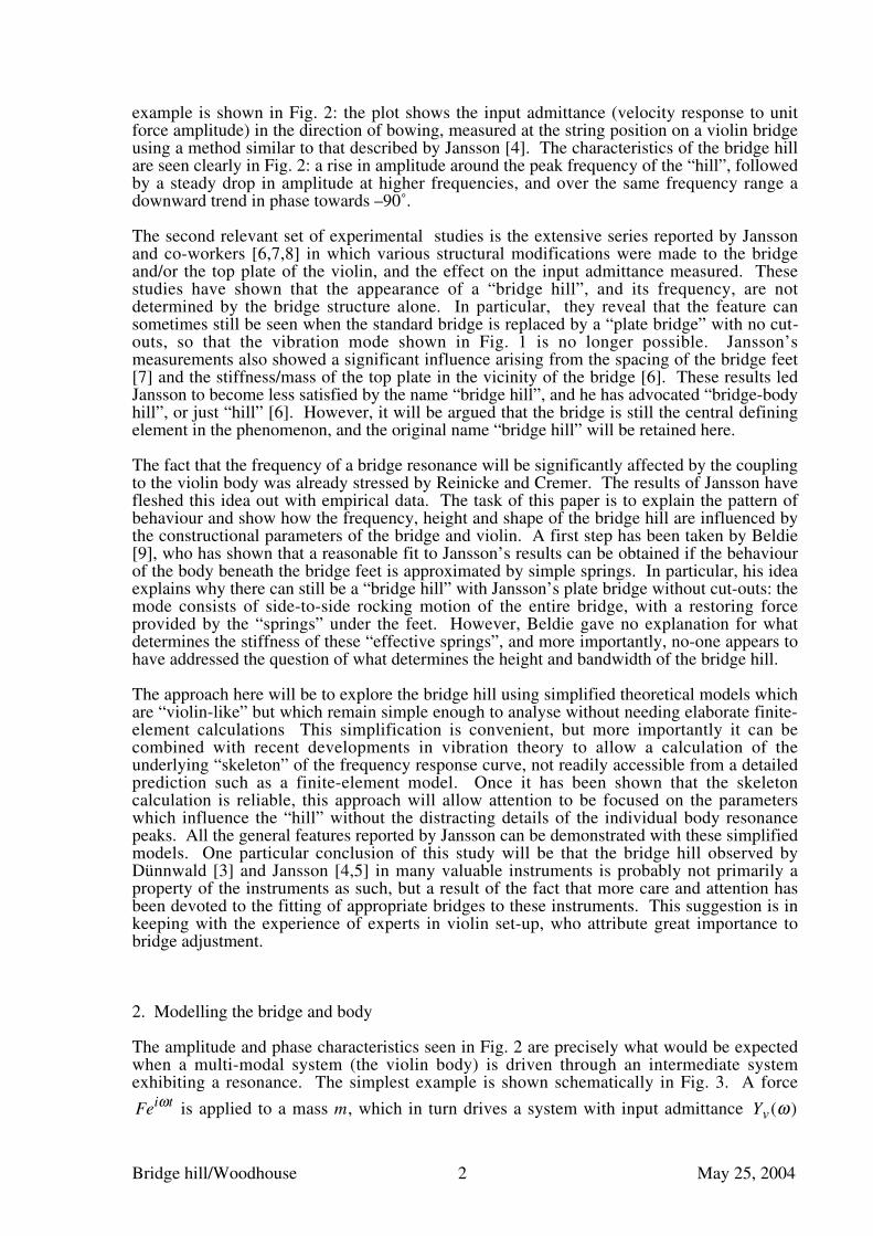
example is shown in Fig. 2: the plot shows the input admittance (velocity response to unitforce amplitude) in the direction of bowing, measured at the string position on a violin bridgeusing a method similar to that described by Jansson [4]. The characteristics of the bridge hillare seen clearly in Fig. 2: a rise in amplitude around the peak frequency of the “hill”, followedby a steady drop in amplitude at higher frequencies, and over the same frequency range adownward trend in phase towards –90˚.

The second relevant set of experimental studies is the extensive series reported by Janssonand co-workers [6,7,8] in which various structural modifications were made to the bridgeand/or the top plate of the violin, and the effect on the input admittance measured. Thesestudies have shown that the appearance of a “bridge hill”, and its frequency, are notdetermined by the bridge structure alone. In particular, they reveal that the feature cansometimes still be seen when the standard bridge is replaced by a “plate bridge” with no cut-outs, so that the vibration mode shown in Fig. 1 is no longer possible. Jansson’smeasurements also showed a significant influence arising from the spacing of the bridge feet[7] and the stiffness/mass of the top plate in the vicinity of the bridge [6]. These results ledJansson to become less satisfied by the name “bridge hill”, and he has advocated “bridge-bodyhill”, or just “hill” [6]. However, it will be argued that the bridge is still the central definingelement in the phenomenon, and the original name “bridge hill” will be retained here.

The fact that the frequency of a bridge resonance will be significantly affected by the couplingto the violin body was already stressed by Reinicke and Cremer. The results of Jansson havefleshed this idea out with empirical data. The task of this paper is to explain the pattern ofbehaviour and show how the frequency, height and shape of the bridge hill are influenced bythe constructional parameters of the bridge and violin. A first step has been taken by Beldie[9], who has shown that a reasonable fit to Jansson’s results can be obtained if the behaviourof the body beneath the bridge feet is approximated by simple springs. In particular, his ideaexplains why there can still be a “bridge hill” with Jansson’s plate bridge without cut-outs: themode consists of side-to-side rocking motion of the entire bridge, with a restoring forceprovided by the “springs” under the feet. However, Beldie gave no explanation for whatdetermines the stiffness of these “effective springs”, and more importantly, no-one appears tohave addressed the question of what determines the height and bandwidth of the bridge hill.

The approach here will be to explore the bridge hill using simplified theoretical models whichare “violin-like” but which remain simple enough to analyse without needing elaborate finite-element calculations This simplification is convenient, but more importantly it can becombined with recent developments in vibration theory to allow a calculation of theunderlying “skeleton” of the frequency response curve, not readily accessible from a detailedprediction such as a finite-element model. Once it has been shown that the skeletoncalculation is reliable, this approach will allow attention to be focused on the parameterswhich influence the “hill” without the distracting details of the individual body resonancepeaks. All the general features reported by Jansson can be demonstrated with these simplifiedmodels. One particular conclusion of this study will be that the bridge hill observed byDünnwald [3] and Jansson [4,5] in many valuable instruments is probably not primarily aproperty of the instruments as such, but a result of the fact that more care and attention hasbeen devoted to the fitting of appropriate bridges to these instruments. This suggestion is inkeeping with the experience of experts in violin set-up, who attribute great importance tobridge adjustment.

2. Modelling the bridge and body

The amplitude and phase characteristics seen in Fig. 2 are precisely what would be expectedwhen a multi-modal system (the violin body) is driven through an intermediate systemexhibiting a resonance. The simplest example is shown schematically in Fig. 3. A force

Feiωt is applied to a mass m, which in turn drives a system with input admittance Yv (ω )


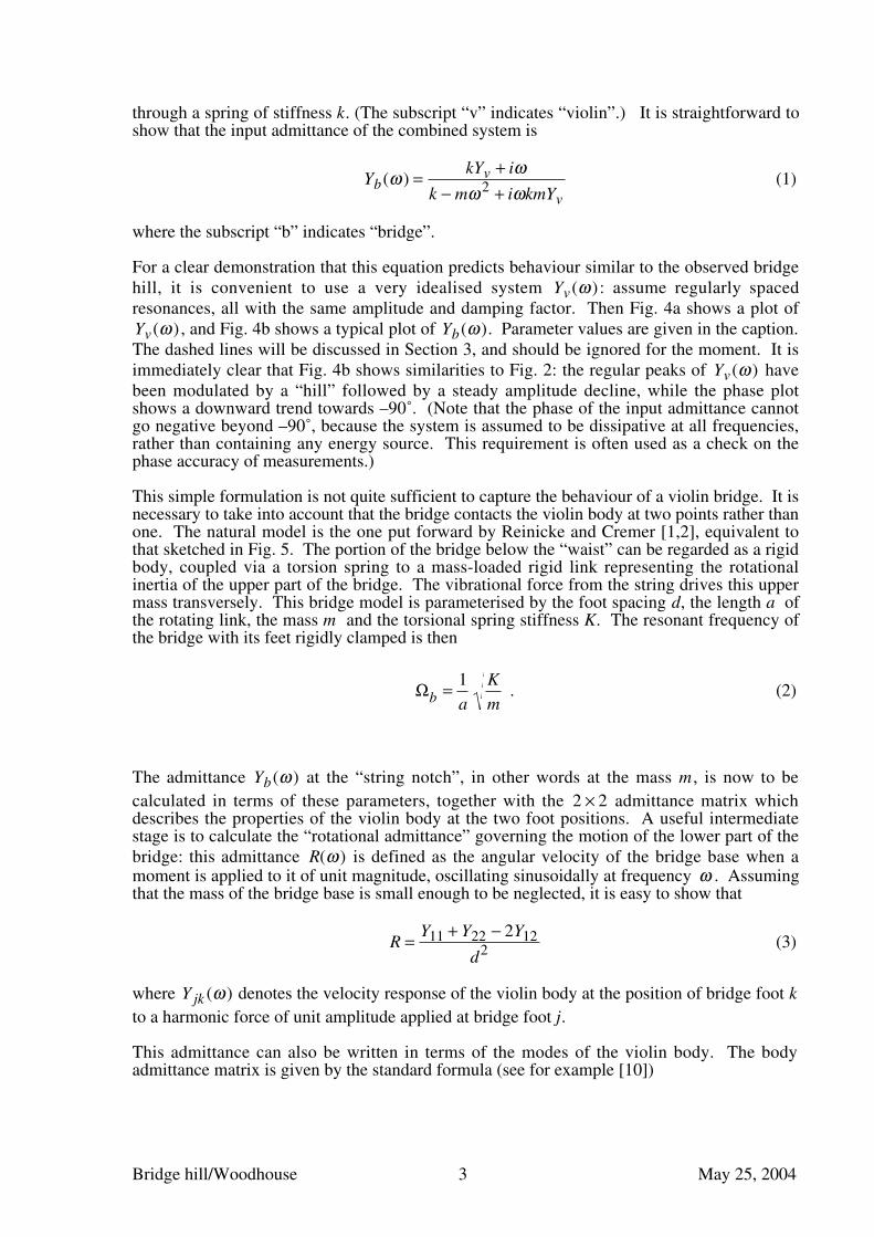
through a spring of stiffness k. (The subscript “v” indicates “violin”.) It is straightforward toshow that the input admittance of the combined system is

Yb(ω ) =kYv + iω

k − mω 2 + iωkmYv

(1)

where the subscript “b” indicates “bridge”.

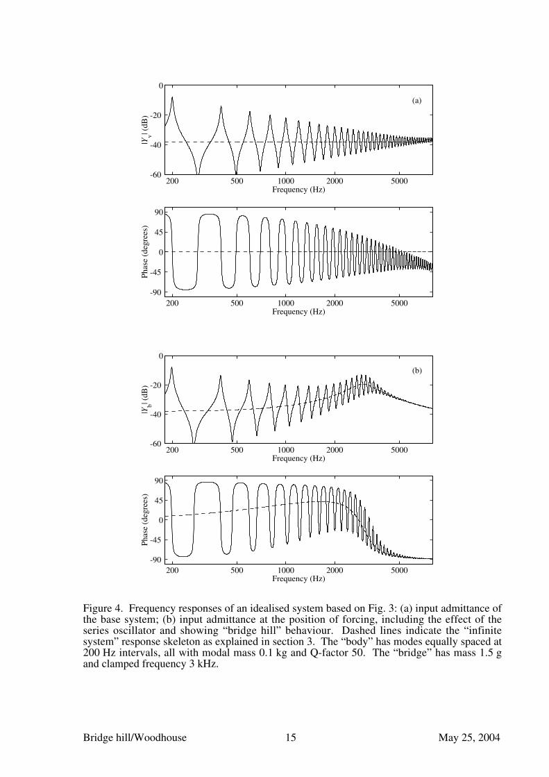
For a clear demonstration that this equation predicts behaviour similar to the observed bridgehill, it is convenient to use a very idealised system Yv (ω ) : assume regularly spacedresonances, all with the same amplitude and damping factor. Then Fig. 4a shows a plot ofYv (ω ) , and Fig. 4b shows a typical plot of Yb(ω ). Parameter values are given in the caption.The dashed lines will be discussed in Section 3, and should be ignored for the moment. It isimmediately clear that Fig. 4b shows similarities to Fig. 2: the regular peaks of Yv (ω ) havebeen modulated by a “hill” followed by a steady amplitude decline, while the phase plotshows a downward trend towards –90˚. (Note that the phase of the input admittance cannotgo negative beyond –90˚, because the system is assumed to be dissipative at all frequencies,rather than containing any energy source. This requirement is often used as a check on thephase accuracy of measurements.)

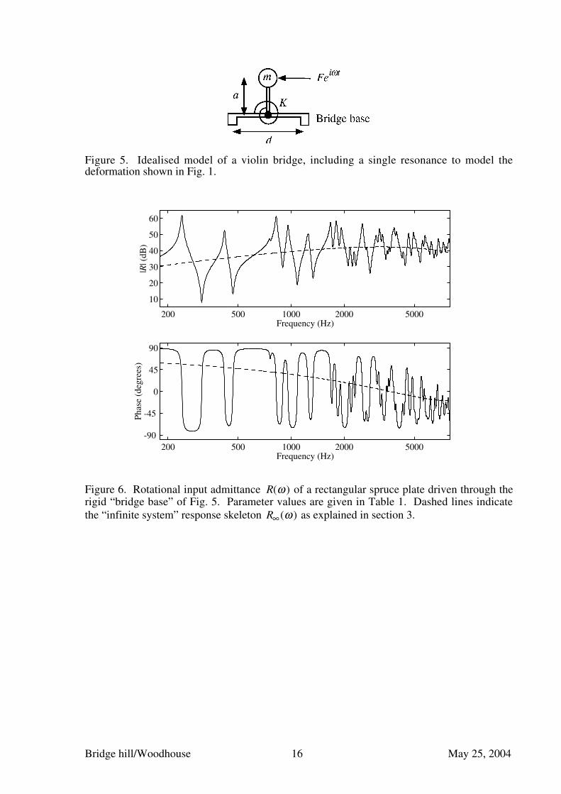
This simple formulation is not quite sufficient to capture the behaviour of a violin bridge. It isnecessary to take into account that the bridge contacts the violin body at two points rather thanone. The natural model is the one put forward by Reinicke and Cremer [1,2], equivalent tothat sketched in Fig. 5. The portion of the bridge below the “waist” can be regarded as a rigidbody, coupled via a torsion spring to a mass-loaded rigid link representing the rotationalinertia of the upper part of the bridge. The vibrational force from the string drives this uppermass transversely. This bridge model is parameterised by the foot spacing d, the length a ofthe rotating link, the mass m and the torsional spring stiffness K. The resonant frequency ofthe bridge with its feet rigidly clamped is then

Ωb =1

a

K

m . (2)

The admittance Yb(ω ) at the “string notch”, in other words at the mass m , is now to be

calculated in terms of these parameters, together with the 2 × 2 admittance matrix whichdescribes the properties of the violin body at the two foot positions. A useful intermediatestage is to calculate the “rotational admittance” governing the motion of the lower part of thebridge: this admittance R(ω ) is defined as the angular velocity of the bridge base when amoment is applied to it of unit magnitude, oscillating sinusoidally at frequency ω . Assumingthat the mass of the bridge base is small enough to be neglected, it is easy to show that

R =Y11 + Y22 − 2Y12

d2 (3)

where Y jk (ω ) denotes the velocity response of the violin body at the position of bridge foot k

to a harmonic force of unit amplitude applied at bridge foot j.

This admittance can also be written in terms of the modes of the violin body. The bodyadmittance matrix is given by the standard formula (see for example [10])


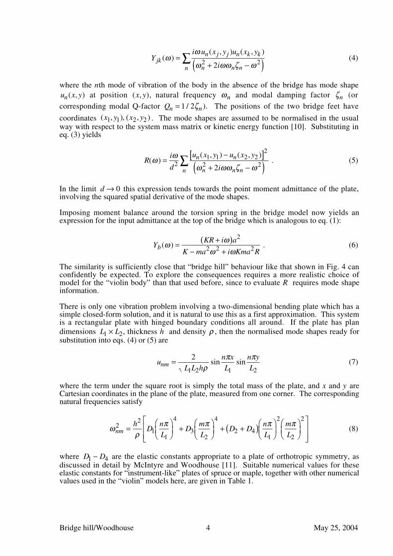
Y jk (ω ) =iω un(x j , y j )un(xk , yk )

ωn2 + 2iωωnζn − ω 2( )n

∑ (4)

where the nth mode of vibration of the body in the absence of the bridge has mode shapeun(x, y) at position (x, y), natural frequency ωn and modal damping factor ζn (or

corresponding modal Q-factor Qn = 1 / 2ζn ). The positions of the two bridge feet have

coordinates (x1, y1), (x2 , y2 ) . The mode shapes are assumed to be normalised in the usualway with respect to the system mass matrix or kinetic energy function [10]. Substituting ineq. (3) yields

R(ω ) =iωd2

un(x1, y1) − un(x2 , y2 )[ ]2ωn

2 + 2iωωnζn − ω 2( )n

∑ . (5)

In the limit d → 0 this expression tends towards the point moment admittance of the plate,involving the squared spatial derivative of the mode shapes.

Imposing moment balance around the torsion spring in the bridge model now yields anexpression for the input admittance at the top of the bridge which is analogous to eq. (1):

Yb(ω ) =KR + iω( )a2

K − ma2ω 2 + iωKma2R . (6)

The similarity is sufficiently close that “bridge hill” behaviour like that shown in Fig. 4 canconfidently be expected. To explore the consequences requires a more realistic choice ofmodel for the “violin body” than that used before, since to evaluate R requires mode shapeinformation.

There is only one vibration problem involving a two-dimensional bending plate which has asimple closed-form solution, and it is natural to use this as a first approximation. This systemis a rectangular plate with hinged boundary conditions all around. If the plate has plandimensions L1 × L2, thickness h and density ρ , then the normalised mode shapes ready forsubstitution into eqs. (4) or (5) are

unm =2

L1L2hρsin

nπx

L1sin

nπy

L2(7)

where the term under the square root is simply the total mass of the plate, and x and y areCartesian coordinates in the plane of the plate, measured from one corner. The correspondingnatural frequencies satisfy

ωnm2 =

h2

ρD1

nπL1

4

+ D3mπL2

4

+ D2 + D4( ) nπL1

2mπL2

2

(8)

where D1 − D4 are the elastic constants appropriate to a plate of orthotropic symmetry, asdiscussed in detail by McIntyre and Woodhouse [11]. Suitable numerical values for theseelastic constants for “instrument-like” plates of spruce or maple, together with other numericalvalues used in the “violin” models here, are given in Table 1.


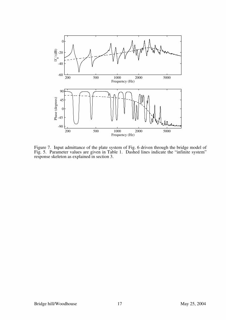
Using this model, the “rotational admittance” R is plotted in Fig. 6 and the input admittance atthe bridge top is shown in Fig. 7. The dashed lines in these plots will be explained in the nextsection. Figure 6 shows no very strong trend with frequency, somewhat similar to Fig. 4a,while Fig. 7 shows a clear bridge hill. Also, the absolute level of the admittance in Fig. 7 issimilar to that seen in Fig. 2, confirming that this simple model has broadly violin-likebehaviour. The aspect of this model which is most obviously unrealistic is not immediatelyapparent from these plots. Because the “bridge” has been placed symmetrically with respectto the mid-line of the plate, many of the plate modes do not contribute to R. These modes havemotion that is symmetrical at the two bridge feet so that, from eq. (5), their contribution to Ris zero. In a real violin, the presence of the bass bar and soundpost destroy the symmetry ofthe structure, so that potentially all modes could contribute to R.

It is not easy to incorporate a bass bar into the idealised model used here, but a representationof the soundpost is quite simple to achieve. The model can be extended to include tworectangular plates, representing the top and back of the violin. Both will have the same plangeometry, and will have hinged boundaries along all edges. The two plates can then becoupled together at a chosen point by a massless, rigid link representing the soundpost. Suchpoint-coupled systems are easily modelled using appropriate combinations of the admittances.If the only requirement were the driving-point admittance Ycoup of the coupled plates at the

“soundpost” position, it would be given simply by

1

Ycoup

=1

Y1+

1

Y2(9)

where Y1, Y2 are the input admittances of the two uncoupled systems at the same position.This familiar formula expresses the fact that the displacements of the two coupled systems arethe same at the coupling point, while the total applied force is the sum of the forces applied tothe two separate subsystems.

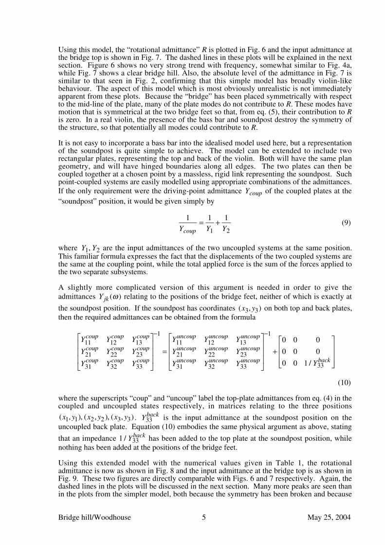
A slightly more complicated version of this argument is needed in order to give theadmittances Y jk (ω ) relating to the positions of the bridge feet, neither of which is exactly at

the soundpost position. If the soundpost has coordinates (x3, y3) on both top and back plates,then the required admittances can be obtained from the formula

Y11coup

Y12coup

Y13coup

Y21coup

Y22coup

Y23coup

Y31coup

Y32coup

Y33coup

−1

=

Y11uncoup

Y12uncoup

Y13uncoup

Y21uncoup

Y22uncoup

Y23uncoup

Y31uncoup

Y32uncoup

Y33uncoup

−1

+0 0 0

0 0 0

0 0 1 / Y33back

(10)

where the superscripts “coup” and “uncoup” label the top-plate admittances from eq. (4) in thecoupled and uncoupled states respectively, in matrices relating to the three positions

(x1, y1), (x2 , y2 ), (x3, y3) . Y33back is the input admittance at the soundpost position on the

uncoupled back plate. Equation (10) embodies the same physical argument as above, stating

that an impedance 1 / Y33back has been added to the top plate at the soundpost position, while

nothing has been added at the positions of the bridge feet.

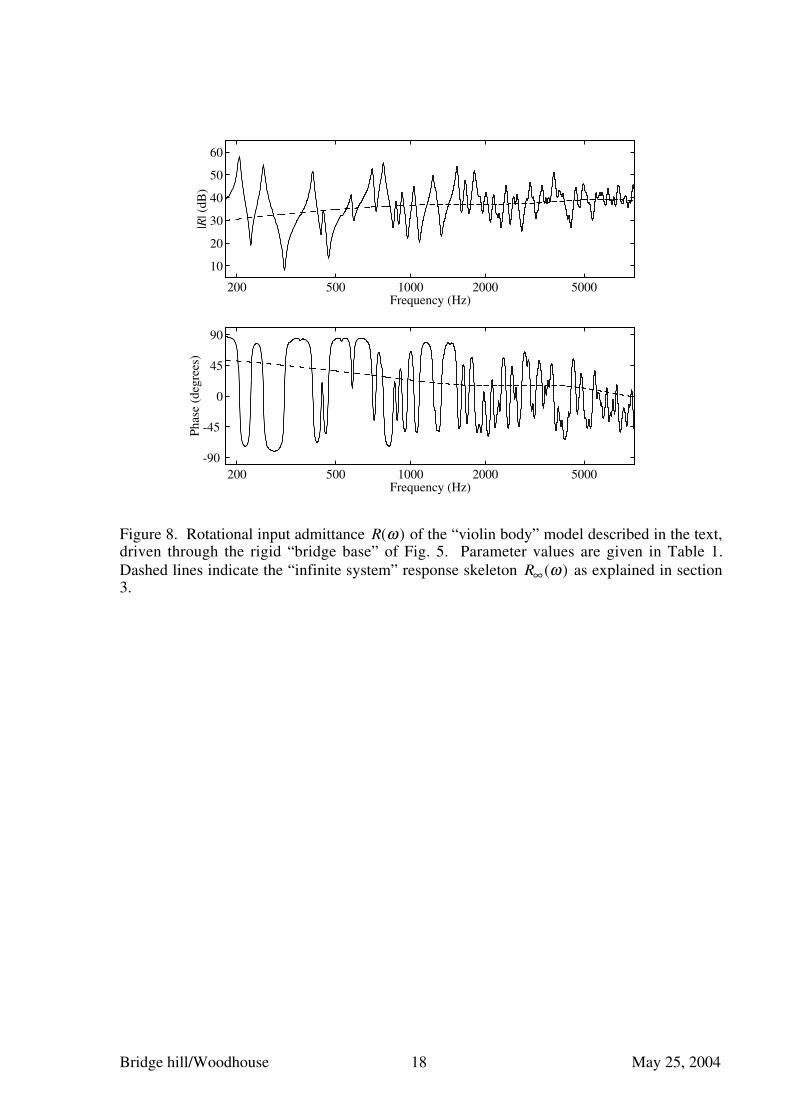
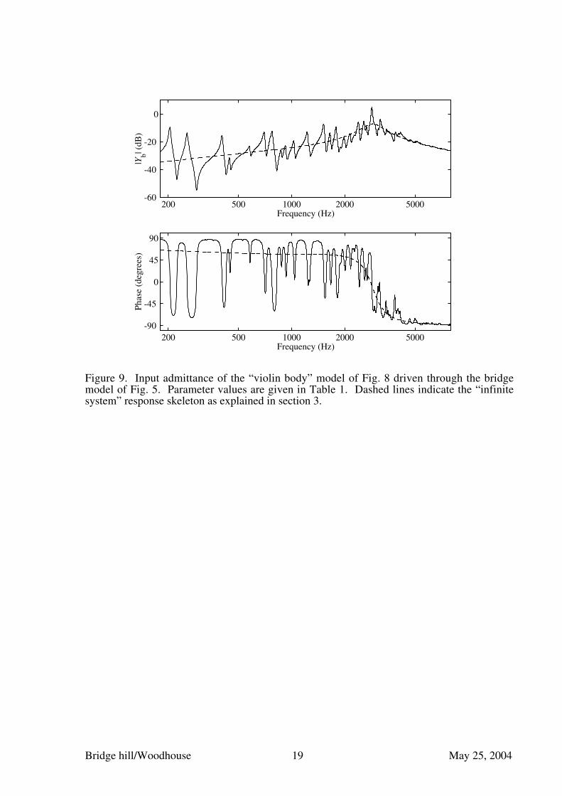
Using this extended model with the numerical values given in Table 1, the rotationaladmittance is now as shown in Fig. 8 and the input admittance at the bridge top is as shown inFig. 9. These two figures are directly comparable with Figs. 6 and 7 respectively. Again, thedashed lines in the plots will be discussed in the next section. Many more peaks are seen thanin the plots from the simpler model, both because the symmetry has been broken and because


the back plate has introduced additional resonances of its own. The trends are generallysimilar, with a clear bridge hill seen in Fig. 9. Notice that the hill is rather higher andnarrower than in Fig. 7. This extended model will be used to investigate the influence on thebridge hill of various parameters relating to the bridge and to the “violin body”.

It is interesting to compare Fig. 9 with the measured admittance in Fig. 2. This reveals thatthe general levels are quite similar except near the hill, which is a little too prominent in thisparticular simulation. However, it will be seen in section 4 that the parameter values of thebridge model could readily be altered to achieve a closer match of the hill. The other obviousdifference between Figs. 2 and 9 is that the flat-plate “violin” has a higher density ofresonances at low frequencies than the real violin. The reason for this probably lies mainly inthe arched plates of the real violin: curved shells such as cylinders have low modal densitybelow the “ring frequency” [12], but at higher frequencies they tend towards the same modaldensity as a flat plate of the same area. The ring frequency in Hz is given by c / 2πR , whereR is the radius of the cylinder and c is the compressional wave speed. It is not influenced bythe thickness of the shell. There is no single “ring frequency” for the complex geometry of aviolin plate, but simple estimates based on typical axial or transverse radii of curvature of aviolin top, and the corresponding wave speeds of spruce, yield values of the order of 1–2 kHz.At frequencies of relevance to the bridge hill, the flat-plate model should have similar modaldensity to the real violin. The model seems good enough that one might hope to obtainplausible bridge-hill shapes with numerical values of bridge parameters close to thosemeasured from real bridges.

3. The response skeleton

Before looking at parameter studies, though, it is desirable to find a way to focus on theunderlying hill without the distracting details of the individual body modes. This can be donereadily for this simple model, by using an approach known in different guises as “Skudrzyk’smean value method” [13] or “fuzzy structure theory” [14]. Skudrzyk’s argument is the mostdirect for the present purpose. The key insight is that, from eq. (4), the height of an isolatedmodal peak is proportional to 1 / ζn , while the level at an antiresonance dip is proportional to

ζn . It follows that the mean level of a logarithmic plot follows the geometric mean of thesetwo, and is thus independent of damping. If the damping were increased, the peaks and dipswould blur out and all admittance curves would tend towards smooth “skeleton” curvesrepresenting the logarithmic mean of the original curves.

There is a physically appealing way to visualise the effect of increasing the damping. When aforce is applied at a point on the structure, it generates a “direct field” consisting of outward-travelling waves. In time these will reflect from the various boundaries and return. Modalpeaks will occur at frequencies where the reflections combine in phase-coherent ways.Antiresonances occur when the sum of reflected waves systematically cancels the originaldirect field. But at an “average” frequency, where neither of these coherent phase effectsoccurs, the reflected waves from the various boundaries tend to arrive in random phases andto cancel each other out, leaving the direct field to dominate the response. If damping isincreased, the influence of reflections decreases. In the limit of high damping, the desired“skeleton” of the admittance is given by the direct field alone.

The effect is thus the same as if the plate boundaries had been pushed further away until thesystem becomes infinitely large. This gives a simple recipe to find skeleton curves for themodels discussed above: the rectangular top and back plates are replaced by infinite plateswith the same material properties and thicknesses. The vibration of a point-driven infiniteplate has a simple closed-form solution. For a plate of isotropic material of density ρ ,Young’s modulus E, Poisson’s ratio ν and thickness h the driving-point admittance is


Y∞(ω ,0) =1

4h23(1 − ν2 )

Eρ , (11)

which represents a pure resistance: it is real and independent of frequency. For response at apoint a distance r from the driven point, the transfer admittance is

Y∞(ω ,r) =1

4h23(1 − ν2 )

EρH0

(2)(kr) − H0(2)(−ikr)[ ] (12)

where the wavenumber k is given by

k4 =12ρ(1 − ν2 )ω 2

Eh2 (13)

and H0(2) is the Hankel function of the second kind of order zero [15].

For a plate of orthotropic material like wood the behaviour is somewhat more complicated,but a standard approximation is sufficiently good for the present purpose. If it is assumed that

D2 + D4 = 2 D1D3 (14)

then the plate is equivalent to an isotropic one provided distance x “along the grain” is scaledrelative to distance y “across the grain” according to

x = x D3 / D1( )1/4. (15)

The equivalent result to eq. (12) is then

Y∞(ω ) =1

8h2 ρ D1D3

H0(2)(kr) − H0

(2)(−ikr)[ ] (16)

where

k4 =ρω 2

D3h2 (17)

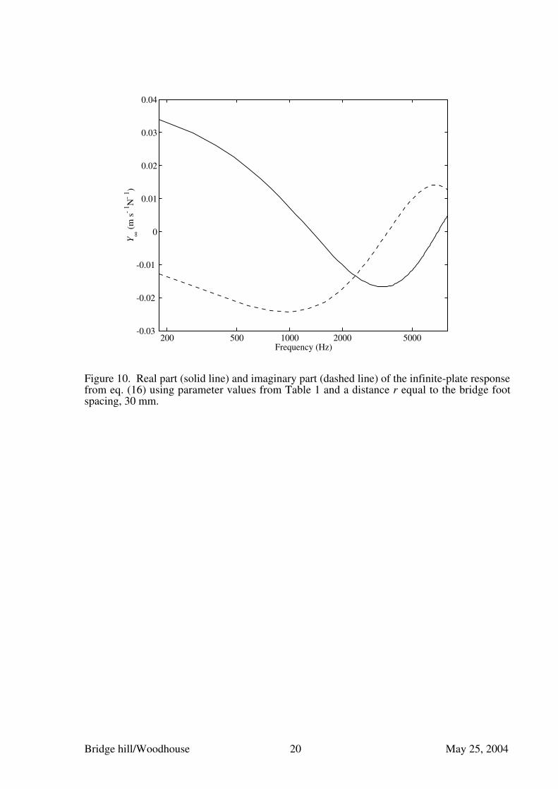
and r is calculated using x, y( ). To illustrate the behaviour predicted by eq. (16), Fig. 10

shows the real and imaginary parts of Y∞ for the parameters of the spruce plate used in themodels in the previous section, and a value of r equal to the bridge-foot spacing assumedthere.

The calculations of the previous section can be readily repeated using these infinite-plateadmittances in place of the finite-plate results used before: in particular, eq. (10) can still beused to give a model which allows for the soundpost, but treats both the top and back plates asinfinite in extent. The results are shown as dashed lines in Figs. 4, 6–9. It is clear that thesedashed lines do indeed follow accurately the mean trend of the logarithmic amplitude and thephase, and also that they reveal the form of the bridge hill in Figs. 4b, 7 and 9. The skeletoncurves based on this infinite-plate modelling have been found to show similar accuracy over a


wide range of parameter values. It seems clear that, to study the bridge hill, it will besufficient to study these simple skeleton curves.

Some conclusions can be drawn immediately. The skeleton of the input admittance at thebridge is given by eq. (6) with R replaced by the “skeleton” value R∞ . It is plausible, andconfirmed by the dashed lines in Figs. 6 and 8, that this value varies only slowly withfrequency. Substituting a constant value appropriate to the general vicinity of the bridge hill,eq. (6) shows that the form of the hill is determined by complex poles which are the roots of

ω 2 − iωR∞K − Ωb2 = 0. (18)

If R∞ is real, this takes the familiar form of a damped harmonic oscillator which representsthe bridge resonance damped by radiation through the feet into the infinite plate system. Theeffective damping factor ζb of this “hill oscillator” can be written in several equivalent forms:

ζb = R∞K / 2Ωb = R∞ma2Ωb / 2 = R∞a Km / 2 . (19)

If ζb is small the bridge hill will appear as a tall, narrow peak close to the clamped bridge

frequency Ωb. As ζb increases, the bridge hill moves down somewhat in frequency and the

peak becomes broader and lower. If ζb reaches unity the bridge hill becomes criticallydamped so that it ceases to be visible as a “hill” and simply becomes a low-pass filter.Equation (19) thus shows how the various model parameters combine to determine the heightand bandwidth of the bridge hill, an aspect which has not been much discussed in theliterature of the subject.

If R∞ is complex the interpretation of eq. (18) is a little less obvious. An estimate of thedamping factor of the hill can probably be obtained from eq. (19) by replacing R∞ with

Re R∞( ), but the imaginary part of R∞ will contribute a reactive effect which will shift the

frequency of the hill away from the clamped frequency Ωb. This is the physical origin of theeffect observed by Jansson [6,8], and idealised by Beldie in terms of effective springs beneaththe bridge feet [9]. Indeed, it is simple to obtain from eq. (18) an estimate of the hillfrequency when the flexible bridge is replaced with a rigid “plate bridge” as in Jansson’sexperiments [6]. Rewriting eq. (18) in the form

ω 2 − iωR∞K − K / (ma2 ) = 0 (20)

then allowing K → ∞ , it is clear that the first term of eq. (20) becomes negligible in thefrequency range of interest, and the effective pole frequency is given by the other two terms as

ω ≈ i / ma2R∞( ) . (21)

This expression clearly shows the hill frequency arising under these limiting conditions from abalance between (rotational) stiffness provided by the violin body, and inertia provided by thebridge.

To look a little more closely at the behaviour when R∞ is complex, the flat-plate model can beused to suggest appropriate numerical values to explore. Figure 11 shows the real andimaginary parts of R∞ corresponding to Fig. 8. For a bridge hill in the vicinity of 2.5 kHz, it

seems reasonable to take Re R∞( ) = 100 rad m-1s-1N-1 and to explore a range of Im R∞( ) ofthe same order of magnitude. Figure 12 shows the resulting variation of hill frequency and


loss factor, obtained by solving eq. (18) exactly. The frequency can be raised or lowered

relative to the clamped frequency (3 kHz here), depending on the sign of Im R∞( ): thereseems to be no physical reason why it should necessarily be positive (and hence “spring-

like”). The loss factor turns out to be influenced very little by Im R∞( ): it remains close to the

value given by eq. (19) with R∞ replaced by Re R∞( ), shown as the dashed line.

4. Parameter studies

4.1. Parameters of the bridge

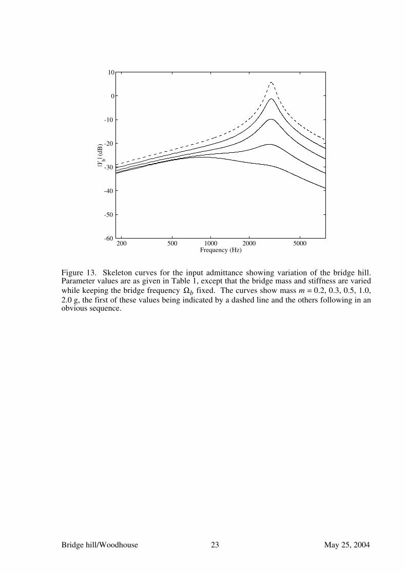
The flat-plate model does not by any means represent all relevant features of the violin body,but it contains enough detail that considerable insight of a semi-quantitative nature can begained by varying the parameters of the model. Sets of “skeleton” curves will be shown toillustrate how the bridge hill is affected by various changes which have direct analogues inviolin-making practice. First, parameters relating to the bridge will be tested. Figure 13shows the effect of varying the mass and stiffness of the bridge in such a way that the ratio,and hence the clamped resonance frequency, is kept constant. The behaviour is as anticipatedfrom eq. (19): the main effect is that the damping factor of the hill resonance varies over awide range with relatively small changes in the mass and stiffness. The peak frequency of thehill remains close to the clamped frequency throughout: for these particular parameter values,as seen in Fig. 11, the reactive component of R∞ is small in the relevant frequency range.From the perspective of a violin maker, this figure shows the effect of adjusting the bridge bythinning the entire structure: the mass and the stiffness will both vary in proportion to thethickness, and the ratio will remain constant. Such adjustment seems to give a very directway to change the height and bandwidth of the bridge hill.

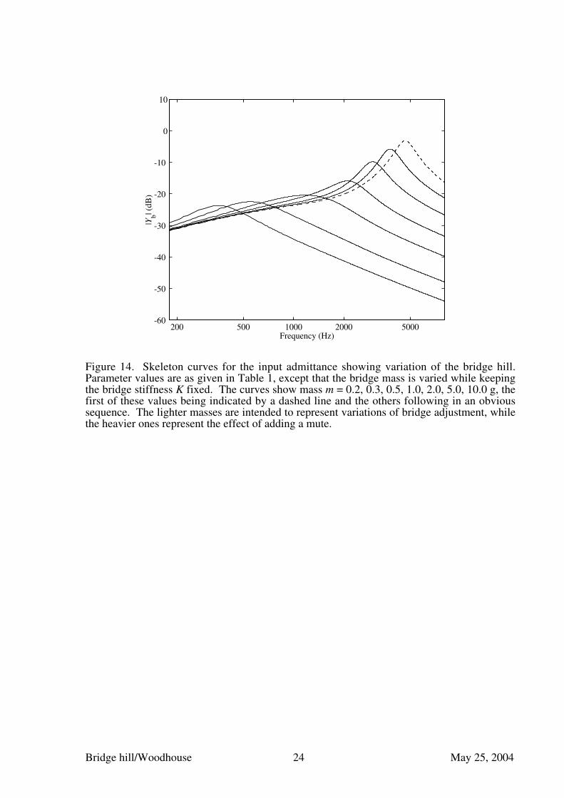
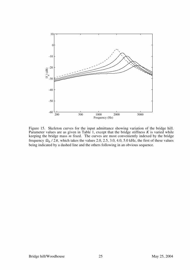
Figures 14 and 15 show the effect of varying the bridge-top mass keeping the stiffnessconstant, and conversely varying the stiffness keeping the mass constant. Both correspond torealistic bridge adjustment procedures: the mass is determined by the thickness of the topportion of the bridge (and by the bridge height and choice of wood), while the stiffness can bevaried independently by trimming around the cutouts. In addition, Fig. 14 illustrates the effectof adding a mute to the violin bridge: the range of masses explored is sufficiently wide tocover variations of bridge shaping and typical mutes. As anticipated, both figures show acombination of varying hill frequency and bandwidth. Taken in combination with Figure 11,it would appear that by judicious bridge adjustment the hill frequency and bandwidth couldboth be placed wherever required on this simplified violin body. On a violin in which R∞showed a bigger reactive component there might be limits on the range over which thefrequency and bandwidth could be adjusted (as shown by Jansson’s test with the plate bridge[6]).

Finally, Jansson has shown an interesting series of measurements using bridges with differentfoot spacings d [7]. This experiment is simulated, approximately, in Fig. 16. Results are seenwhich qualitatively mirror the experimental findings. Decreasing the foot spacing reduces thepeak frequency of the hill, by changing R∞ . Interestingly, for this model at least, the hillbandwidth varies at the same time in a non-obvious way. As the foot spacing is reduced fromits normal value, the bandwidth increases to a maximum with a foot spacing around 20 mm,then decreases again when the spacing is reduced further. Note that the clamped bridgeresonance remains at 3 kHz throughout this series of simulations, so that the shift in hillfrequency is entirely due to changes in the reactive component of R∞ .


4.2. Parameters of the violin body

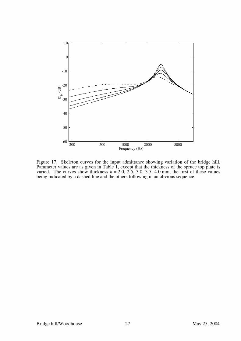
In a similar way, the model can be used to explore changes in the parameters of the violinbody, keeping the bridge unchanged. Figures 17 and 18 show the influence of the thicknessof the top and back plates respectively. The set of thicknesses tested were the same in bothcases, 2–4 mm: in reality, a violin top plate would usually have a thickness in the bridgeregion towards the lower end of this range [16], while the back plate near the soundpostposition would have a thickness at the upper end of the range. The results show similar tendsin both cases, but not surprisingly the hill is affected much more sensitively by the topthickness than by the back thickness. A thinner top, and to a lesser extent a thinner back, hasthe effect of reducing the hill frequency and increasing its bandwidth. It also has a significanteffect on the level of the skeleton curve at low frequencies, but it is an open question whetherthis aspect of the results carries over to a real violin body with its arched plates, since thefrequencies in question are low enough that one would expect curvature to matter.

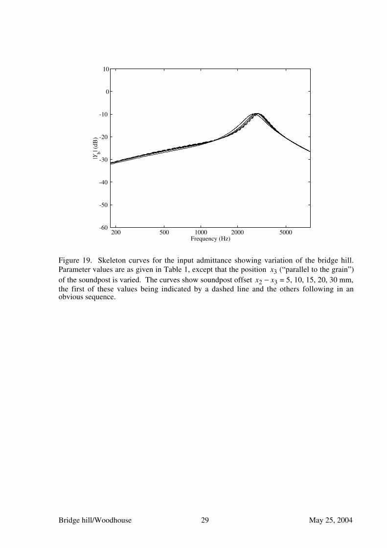
Finally, in Fig. 19 the effect of soundpost position is explored. The soundpost is moved alonga line behind the “treble” foot of the bridge, parallel to the grain of the top plate. The distancebetween bridge foot and soundpost is varied in the range 5–30 mm. Ordinarily, the soundpostposition would be near the lower end of this range. The results show only a rather slightinfluence on the bridge hill, one which could easily be compensated by small adjustments tothe bridge. The well-known sensitivity of the sound of a violin to the position of thesoundpost does not seem to be associated to any great degree with changes to the bridge hill,at least within this simplified model.

5. Conclusions and implications for violin makers

It has been shown that Reinicke’s model for the deformation of a violin bridge in its lowest in-plane resonance [1,2] can be combined with a very simple model of violin body vibration togive a system which can elucidate the various published measurements relating to the bridgehill in the input admittance of a violin [6,7,8]. By replacing the finite plates in the body modelby infinite plates, the calculation can directly yield the “skeleton” curve which underlies thebridge hill. Using the skeleton curve, the frequency and bandwidth of the hill were shown tovary in a simple and predictable way with the parameters which determine the behaviour ofthe bridge and the violin body model. There is obvious scope for experiments to test thepredictions of this study by making controlled adjustments to bridges and measuring the effecton the input admittance and the bridge hill.

The results of this study are of direct interest to violin makers. The bridge model, and theformula (19) for the effective loss factor of the hill, is quite robust. Although the body modelused here was highly schematic, the general conclusions about the effect of bridge adjustmenton the frequency, height and bandwidth of the hill should carry over directly to the behaviourof a bridge on a real violin. If a “normal” bridge hill is desired (and one should not forget thatthe evidence for the significance of the hill comes only from correlation studies, not frompsychoacoustical tests), then it should always be possible to create one on any reasonablyconventional violin by suitable bridge adjustment.

Some instruments place constraints on the potential for shaping the hill by bridge adjustment,because the reactive contribution from the moment admittance of the body ( R∞) has a strongeffect. Jansson’s test instrument seems to be like this, because it showed a fairly normal hilleven with the plate bridge with no cutouts [6]. But Dünnwald’s data for “master instruments”(see Fig. 3 of ref. [3]) suggests that many high-quality instruments are not like this: his plotextends up to 7 kHz with little obvious sign of the low-pass filtering effect of the bridge hill,which should be present even when the hill loss factor exceeds unity so that there is no “hill”as such. It seems likely from the present study that these instruments could all be modified byadjusting their bridges, so that they behaved more like his set of “old Italian violins” (see thesame figure [3]).


If a scientific approach to bridge adjustment were wanted, a possible procedure would be tostart by measuring the input admittance of the violin in question using a Jansson plate bridgein order to calibrate the body behaviour. This would reveal the constraints imposed by thebody behaviour, then it should be possible to adjust a bridge to bring the hill resonance to theright frequency range. At the same time the maker should be careful to monitor the bridgemass, to control the height and bandwidth of the hill. Note that the bridge height and footspacing also have an influence, although in practice there is only limited scope to vary these.Another possible procedure might be to measure directly the 2 × 2 admittance matrix thatdescribes the properties of the violin body at the two foot positions, then calculate the momentadmittance R from eq. (3) and use it to optimise a “virtual bridge design” by computer. Thereal bridge could then be cut while making regular comparisons with the computer model toguide the adjustment process.

To understand why some violins seem to have a greater reactive component of R∞ than otherswould require an extension of the modelling of the violin body. The idea of obtaining theskeleton curve by allowing the top and back plates to become infinite is still valid, but certaindetails of the violin structure are sufficiently close to the bridge that they should be included.The arching and graduation pattern of both plates around the bridge/soundpost area, thecentral portion of the bass bar and the free edges at the f-holes are all strong candidates forinclusion [8]. However, the more remote regions of the plates could be allowed to extend toinfinity in some suitable way, perhaps by using absorbing boundaries in the computation sothat no reflections were generated. If such a model could be analysed, probably using finite-element methods, it would allow the parameter study of section 4 to be extended to otheraspects of the violin structure. Such a model may be a worthwhile subject of future research.


Acknowledgements

The author is grateful to Erik Jansson, Claire Barlow and Robin Langley for usefuldiscussions on this work, to Martin Woodhouse for helping prepare Figure 1 and to HuwRichards for the violin whose response is shown in Fig. 2.

References

[1] L. Cremer: The Physics of the Violin, MIT Press, Cambridge MA 1985. See chapter 9.[2] W. Reinicke: Die Übertragungseigenschaften des Streichinstrumentenstegs. Doctoral

dissertation, Technical University of Berlin, 1973.[3] H. Dünnwald: Deduction of objective quality parameters on old and new violins. J.

Catgut Acoust. Soc. Series 2, 1, 7 (1991)1–5.[4] E. V. Jansson: Admittance measurements of 25 high quality violins. Acustica – Acta

Acustica 83 (1997) 337–341.[5] E. V. Jansson, B. K. Niewczyk: Admittance measurements of violins with high arching.

Acustica - Acta Acustica 83 (1997) 571–574.[6] E. V. Jansson, B. K. Niewczyk: On the acoustics of the violin: bridge or body hill. J.

Catgut Acoust. Soc. Series 2, 3, 7 (1999) 23-27.[7] E. V. Jansson: Violin frequency response — bridge mobility and bridge feet distance.

Submitted to Applied Acoustics (2004).[8] F. Durup, E. V. Jansson: The quest of the violin bridge hill. Submitted to Acustica –

Acta Acustica(2004).[9] I. P. Beldie: About the bridge hill mystery. J. Catgut Acoust. Soc. Series 2, 4, 8 (2003)

9–13.[10] C. H. Hodges, J. Woodhouse: Theories of noise and vibration transmission in complex

structures. Reports on Progress in Physics 49 (1986) 107-170.[11] M. E. McIntyre, J. Woodhouse: On measuring the elastic and damping constants of

orthotropic sheet materials. Acta Metallurgica 36 (1988)1397–1416.[12] E. Szechenyi: Modal densities and radiation efficiencies of unstiffened cylinders using

statistical methods. J. Sound Vib. 19 (1971) 65–81.[13] E. Skudrzyk: The mean-value method of predicting the dynamic response of complex

vibrators. J. Acoust. Soc. Amer. 67 (1980) 1105–1135.[14] R. Ohayon, C. Soize: Structural Acoustics and Vibration, Academic Press, San Diego

CA, 1998. See chapter 15.[15] L. Cremer, M. Heckl, E. E. Ungar: Structure-borne Sound, Springer, Heidelberg 1988.

See section IV, 3d.[16] J. S. Loen: Reverse graduation in fine Cremonese violins. J. Catgut Acoust. Soc. Series

2, 4, 7 (2003) 27-39.


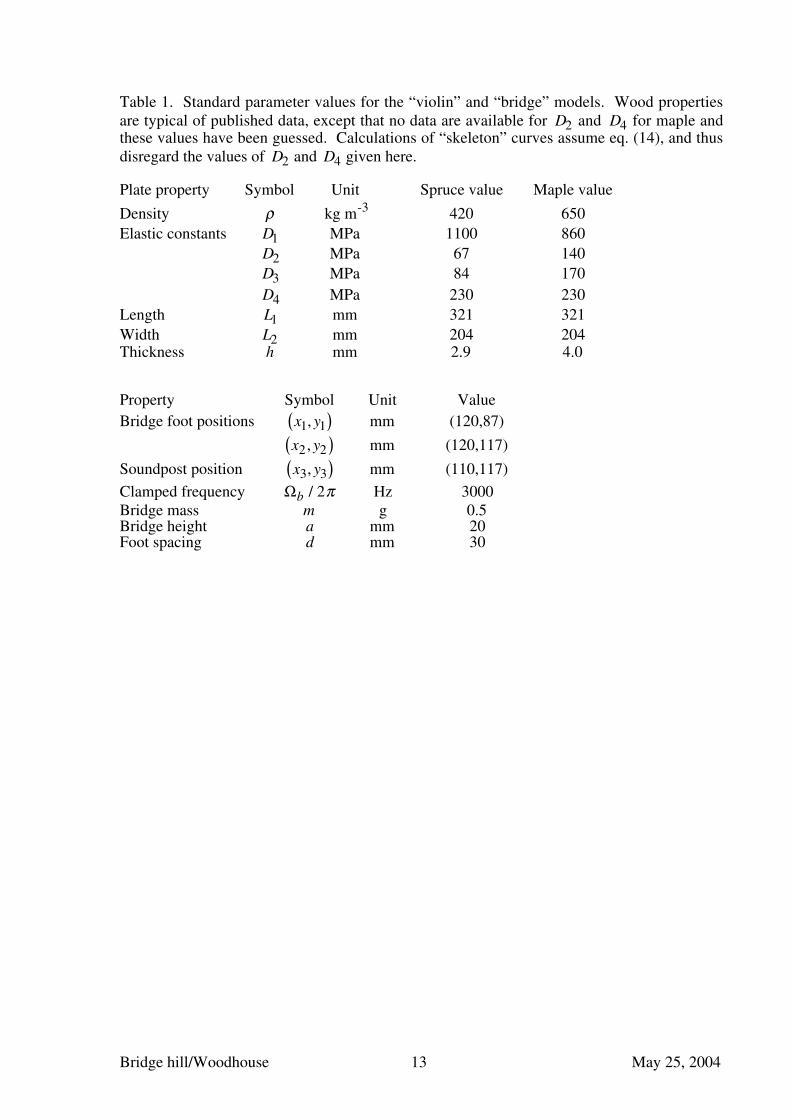
Table 1. Standard parameter values for the “violin” and “bridge” models. Wood propertiesare typical of published data, except that no data are available for D2 and D4 for maple andthese values have been guessed. Calculations of “skeleton” curves assume eq. (14), and thusdisregard the values of D2 and D4 given here.

Plate property Symbol Unit Spruce value Maple value

Density ρ kg m-3 420 650Elastic constants D1 MPa 1100 860

D2 MPa 67 140D3 MPa 84 170

D4 MPa 230 230Length L1 mm 321 321Width L2 mm 204 204Thickness h mm 2.9 4.0

Property Symbol Unit Value

Bridge foot positions x1, y1( ) mm (120,87)

x2 , y2( ) mm (120,117)

Soundpost position x3, y3( ) mm (110,117)

Clamped frequency Ωb / 2π Hz 3000Bridge mass m g 0.5Bridge height a mm 20Foot spacing d mm 30


Figure 1. A violin bridge with an indication of the motion in the lowest in-plane bridgeresonance.

200 500 1000 2000 5000-50

-40

-30

-20

-10

Frequency (Hz)

Adm

itta

nce

(dB

)

200 500 1000 2000 5000-90

-45

0

45

90

Frequency (Hz)

Pha

se (

degr

ees)

Figure 2. Input admittance of a violin, showing a typical bridge hill (in the frequency rangeindicated by the dashed line in the upper plot). The upper plot shows the magnitude in dB re

1 m s−1N−1.

Figure 3. Sketch of a generic system driven through a resonator, as described in the text.


200 500 1000 2000 5000-60

-40

-20

0

Frequency (Hz)

|Yv| (

dB)

(a)

200 500 1000 2000 5000-90

-45

0

45

90

Frequency (Hz)

Pha

se (

degr

ees)

200 500 1000 2000 5000-60

-40

-20

0

Frequency (Hz)

|Yb| (

dB)

(b)

200 500 1000 2000 5000-90

-45

0

45

90

Frequency (Hz)

Pha

se (

degr

ees)

Figure 4. Frequency responses of an idealised system based on Fig. 3: (a) input admittance ofthe base system; (b) input admittance at the position of forcing, including the effect of theseries oscillator and showing “bridge hill” behaviour. Dashed lines indicate the “infinitesystem” response skeleton as explained in section 3. The “body” has modes equally spaced at200 Hz intervals, all with modal mass 0.1 kg and Q-factor 50. The “bridge” has mass 1.5 gand clamped frequency 3 kHz.


Figure 5. Idealised model of a violin bridge, including a single resonance to model thedeformation shown in Fig. 1.

200 500 1000 2000 5000

10

20

30

40

50

60

Frequency (Hz)

|R| (

dB)

200 500 1000 2000 5000-90

-45

0

45

90

Frequency (Hz)

Pha

se (

degr

ees)

Figure 6. Rotational input admittance R(ω ) of a rectangular spruce plate driven through therigid “bridge base” of Fig. 5. Parameter values are given in Table 1. Dashed lines indicatethe “infinite system” response skeleton R∞(ω ) as explained in section 3.


200 500 1000 2000 5000-60

-40

-20

0

Frequency (Hz)

|Yb| (

dB)

200 500 1000 2000 5000-90

-45

0

45

90

Frequency (Hz)

Pha

se (

degr

ees)

Figure 7. Input admittance of the plate system of Fig. 6 driven through the bridge model ofFig. 5. Parameter values are given in Table 1. Dashed lines indicate the “infinite system”response skeleton as explained in section 3.


200 500 1000 2000 5000

10

20

30

40

50

60

Frequency (Hz)

|R| (

dB)

200 500 1000 2000 5000-90

-45

0

45

90

Frequency (Hz)

Pha

se (

degr

ees)

Figure 8. Rotational input admittance R(ω ) of the “violin body” model described in the text,driven through the rigid “bridge base” of Fig. 5. Parameter values are given in Table 1.Dashed lines indicate the “infinite system” response skeleton R∞(ω ) as explained in section3.


200 500 1000 2000 5000-60

-40

-20

0

Frequency (Hz)

|Yb| (

dB)

200 500 1000 2000 5000-90

-45

0

45

90

Frequency (Hz)

Pha

se (

degr

ees)

Figure 9. Input admittance of the “violin body” model of Fig. 8 driven through the bridgemodel of Fig. 5. Parameter values are given in Table 1. Dashed lines indicate the “infinitesystem” response skeleton as explained in section 3.


200 500 1000 2000 5000-0.03

-0.02

-0.01

0

0.01

0.02

0.03

0.04

Frequency (Hz)

Y∞

(m

s-

1 N-

1 )

Figure 10. Real part (solid line) and imaginary part (dashed line) of the infinite-plate responsefrom eq. (16) using parameter values from Table 1 and a distance r equal to the bridge footspacing, 30 mm.


200 500 1000 2000 5000-40

-20

0

20

40

60

80

100

120

Frequency (Hz)

R∞

(ra

d s-

1 N-

1 m-

1 )

Figure 11. Real part (solid line) and imaginary part (dashed line) of the rotational inputadmittance R∞(ω ) of the “skeleton” model described in the text. Parameter values are givenin Table 1.


-100 -80 -60 -40 -20 0 20 40 60 80 1002000

2500

3000

3500

4000

Im(R∞

) (rad s- 1N- 1m- 1)

Hil

l fr

eque

ncy

(Hz) (a)

-100 -80 -60 -40 -20 0 20 40 60 80 1000.186

0.188

0.19

0.192

Im(R∞

) (rad s- 1N- 1m- 1)

Hil

l lo

ss f

acto

r

(b)

Figure 12. Variation of the “hill peak” properties from Eq. (18) with the imaginary part(assumed independent of frequency) of the skeleton rotational input admittance R∞ . The real

part of R∞ has the constant value 100 rad m-1s-1N-1. Plot (a) shows the frequency given by

Re ω( ) ; plot (b) shows the loss factor ζb = Im(ω ) / Re(ω ).


200 500 1000 2000 5000-60

-50

-40

-30

-20

-10

0

10

Frequency (Hz)

|Yb| (

dB)

Figure 13. Skeleton curves for the input admittance showing variation of the bridge hill.Parameter values are as given in Table 1, except that the bridge mass and stiffness are variedwhile keeping the bridge frequency Ωb fixed. The curves show mass m = 0.2, 0.3, 0.5, 1.0,2.0 g, the first of these values being indicated by a dashed line and the others following in anobvious sequence.


200 500 1000 2000 5000-60

-50

-40

-30

-20

-10

0

10

Frequency (Hz)

|Yb| (

dB)

Figure 14. Skeleton curves for the input admittance showing variation of the bridge hill.Parameter values are as given in Table 1, except that the bridge mass is varied while keepingthe bridge stiffness K fixed. The curves show mass m = 0.2, 0.3, 0.5, 1.0, 2.0, 5.0, 10.0 g, thefirst of these values being indicated by a dashed line and the others following in an obvioussequence. The lighter masses are intended to represent variations of bridge adjustment, whilethe heavier ones represent the effect of adding a mute.


200 500 1000 2000 5000-60

-50

-40

-30

-20

-10

0

10

Frequency (Hz)

|Yb| (

dB)

Figure 15. Skeleton curves for the input admittance showing variation of the bridge hill.Parameter values are as given in Table 1, except that the bridge stiffness K is varied whilekeeping the bridge mass m fixed. The curves are most conveniently indexed by the bridgefrequency Ωb / 2π , which takes the values 2.0, 2.5, 3.0, 4.0, 5.0 kHz, the first of these valuesbeing indicated by a dashed line and the others following in an obvious sequence.


200 500 1000 2000 5000-60

-50

-40

-30

-20

-10

0

10

Frequency (Hz)

|Yb| (

dB)

Figure 16. Skeleton curves for the input admittance showing variation of the bridge hill.Parameter values are as given in Table 1, except that the bridge foot spacing d is varied. Thecurves show d = 5, 10, 20, 30, 40 mm, the first of these values being indicated by a dashedline and the others following in an obvious sequence.


200 500 1000 2000 5000-60

-50

-40

-30

-20

-10

0

10

Frequency (Hz)

|Yb| (

dB)

Figure 17. Skeleton curves for the input admittance showing variation of the bridge hill.Parameter values are as given in Table 1, except that the thickness of the spruce top plate isvaried. The curves show thickness h = 2.0, 2.5, 3.0, 3.5, 4.0 mm, the first of these valuesbeing indicated by a dashed line and the others following in an obvious sequence.


200 500 1000 2000 5000-60

-50

-40

-30

-20

-10

0

10

Frequency (Hz)

|Yb| (

dB)

Figure 18. Skeleton curves for the input admittance showing variation of the bridge hill.Parameter values are as given in Table 1, except that the thickness of the maple back plate isvaried. The curves show thickness h = 2.0, 2.5, 3.0, 3.5, 4.0 mm, the first of these valuesbeing indicated by a dashed line and the others following in an obvious sequence.


200 500 1000 2000 5000-60

-50

-40

-30

-20

-10

0

10

Frequency (Hz)

|Yb| (

dB)

Figure 19. Skeleton curves for the input admittance showing variation of the bridge hill.Parameter values are as given in Table 1, except that the position x3 (“parallel to the grain”)

of the soundpost is varied. The curves show soundpost offset x2 − x3 = 5, 10, 15, 20, 30 mm,the first of these values being indicated by a dashed line and the others following in anobvious sequence.

On the “bridge hill” of the violin - · PDF fileOn the “bridge hill”...

Documents

Transcript of On the “bridge hill” of the violin - · PDF fileOn the “bridge hill”...