On the Asset and Liability Management for pension funds: a ...

ISSN:

Número 5 | January 2010

On the Asset and Liability

Management for pension

funds: a multistage

stochastic programming

model and a equilibrium

risk measuring method

Álvaro Veiga

Davi Valladão

Internal Research Reports

Number 5 | January 2010

On the Asset and Liability Management

for pension funds: a multistage

stochastic programming model and a

equilibrium risk measuring method

Álvaro Veiga

Davi Valladão

CREDITS

Publisher:

MAXWELL / LAMBDA-DEE

Sistema Maxwell / Laboratório de Automação de Museus, Bibliotecas Digitais e Arquivos

http://www.maxwell.vrac.puc-rio.br/

Organizers:

Alexandre Street de Aguiar

Delberis Araújo Lima

Cover:

Ana Cristina Costa Ribeiro

http://www.maxwell.vrac.puc-rio.br/

On the Asset and Liability Management for pension

funds: a multistage stochastic programming model and

a equilibrium risk measuring method

Davi Valladao1, Alvaro Veiga

Electrical Engineering Department, Pontifical Catholic University of Rio de Janeiro(PUC-Rio), Rio de Janeiro 22451-900, R.J. Brazil

Abstract

This paper proposes an Asset and Liability Management (ALM) for pen-sion funds via multistage stochastic programming and an equilibrium riskmeasuring method.

The ALM of a pension fund consists in finding the optimal investmentpolicy given the stochastic nature of the asset returns and the liability cashflows. Since it refers to a dynamic portfolio, the most suitable approach wouldbe a multistage stochastic programming model. However, computationalrestrictions don’t allow covering the entire pension fund’s planning horizon.Thus, several articles in literature have proposed an arbitrary fixed capitalrequirement obtained independently on the investment policy adopted toapproximate the effects of the non-considered periods.

Whereas the fund’s actual opportunity cost, we propose a method formeasuring and controlling the equilibrium risk which bootstraps the portfolioreturn scenarios embedded in the optimal solution in order to approximatethe liability discount rate distribution for the periods beyond the consideredplanning horizon.

Key words: Asset Liability Management(ALM), Stochastic Programming,Pension Funds, Solvency Risk, Equilibrium Risk, Bootstrap

1Corresponding author: [email protected]

Preprint submitted to Insurance: Mathematics and Economics November 16, 2009

1. Introduction

The term Asset and Liability Management (ALM) designates the prac-tice of managing a business coordinating decisions and actions taken withrespect to assets and liabilities. The ALM is crucial pursuit for any organiza-tion which receives and invests money in order to fulfill capital requirementsand future cash demands. Moreover, ALM can be defined by the Societyof Actuaries “as an ongoing financial management process of formulating,implementing, monitoring, and revising strategies related to assets and lia-bilities in an attempt to achieve organization’s financial objectives given itsrisk tolerances and other constraints”. According to each context, ALM canhave substantially different aspects. For instance, derivative traders under-stand assets and liabilities as similar entities traded in the financial marketwhile ALM of pension funds is focused on deciding an optimal investmentpolicy while liabilities cannot be changed. The main financial objective ofthe latter financial institution is to ensure the payment of lifelong benefits byinvesting contributions. Hence, the investment policy must assure two condi-tions: equilibrium and liquidity - long and short term solvency, respectively.

The first condition states that the value of the assets should always belarge enough to pay all benefits until the plan extinction. In other words,the solvency capital (the difference between the total asset value and the netpresent liability value) should be positive. The second condition states thatthe investment program should provide enough cash to pay current liabilities,which means that cash level must always be positive. Solvency capital andcash level are affected both by investment policy (decision variables) andasset returns and liability payments (risk factors).

In this paper, we propose a multistage stochastic programming model foran ALM and a new method for measuring and controlling the equilibriumrisk of a pension fund in Brazil. Several articles in literature which proposedstochastic programming models for optimal allocation (Bradley and Crane,1972; Kallberg et al., 1982; Zenios, 1995; Carino and Ziemba, 1998; Kouwen-berg, 2001; Hilli et al., 2007), could only measure the equilibrium risk at theend of the considered planning horizon by comparing the final wealth in eachscenario to a fixed capital requirement obtained independently on the invest-ment policy adopted. However, in an ALM problem, the liabilities discountrate should be taken as the portfolio return (Veiga, 2003), which depend onthe stochastic asset returns and the investment policy. In order to solve thisproblem, we propose an iterative method to measure the equilibrium risk.

2

This method discards the fixed capital requirement approximation and usesthe portfolio return scenarios embedded on the stochastic programming togenerate, via bootstrap, the liability discount rate distribution. Then, we canestimate the net present value distribution of benefits beyond the stochasticprogramming planning horizon and the related insolvency probability.

This paper is organized as follows: After the introduction, we present thestochastic programming model and all processes to produce the necessary in-put to the optimization problem. These processes include a stochastic modelfor economic risk factors, a scenario tree generation method and financialmodels for the assets and liabilities involved. After that, the equilibrium riskmeasuring method will be developed and then the results and conclusionswill be presented.

2. Multistage stochastic programming model

A multistage stochastic programming model is an optimization problemunder uncertainty which the discrete form is solved based on an event tree.Each tree node is associated to a possible state of the system and has aunique predecessor (representing a unique history) and several successors(representing several possible outcomes in the future). In this paper, wedescribe the ALM as a linear maximization problem which, given an initialportfolio allocation, defines the capital movements between the asset classesas the decision variables. The asset classes, indexed as i = 1, ..., 4, are,respectively, stocks, properties, bonds and cash. The model also includesloans, to cover possible cash shortages and transaction costs. Cash balanceand asset inventory constraints are represented, as well as the regulatory andmarket liquidity ones. The objective function is the final wealth expectedutility with a penalty for the insolvent scenarios.

A stage is denoted by t ∈ 0, ..., T and a node related to staget is definedas nt ∈ (Nt−1 + 1) , ..., Nt, where Nt is the number of nodes at stage t. Con-sider N−1 = 0. For illustrative purpose, the event tree has 5 stages and aconditional branching structure given by 1− 10− 6− 6− 4− 4. Indeed, thestages can have different lengths, for instance, the first and the second haveone year, the third has three years, the fourth has five years and the lastone has ten years. This length structure would lead to a 20-year planninghorizon. This structure is represented by Figure 1.

For the optimization model development, first a list of decision variablesand parameters is provided. Parameters are divided in deterministic (with

3

��

��

��

��

�

��

��

��

��

��

��

��

��

��

��

��

Figure 1: Event tree

no uncertainty) and stochastic (risk factors).

∙ Decisions variables

– ci(nt): amount bought of asset class i at node nt

– vi(nt): amount sold of asset class i at node nt

– e(nt): loan obtained at node nt

– ai(nt): amount invested in asset class i at node nt

– y(nT ): positive solvency capital at node nT

– w(nT ): negative solvency capital at node nT

∙ Deterministic parameters

– pe: insolvency penalization

– bo: solvency bonus

– sp: spread between the borrowing rate and the short term interestrate

– ma: maximum stock allocation (%)

4

– ct: transaction cost (%)

– cci: market buying capacity of asset class i

– cvi: market selling capacity of asset class i

– ai: initial allocation of asset class i

– L: capital requirement at the end of planning horizon (t = T )

∙ Stochastic parameters

– l(nt): nominal liability cash flow at node nt

– ri(nt): return of asset class i between two linked nodes nt−1 e nt

2.1. Objective function

The objective function is defined by (1).

NT∑

nT=nT−1+1

p(nT )[bo ⋅ y(nT )− pe ⋅ w(nT )] (1)

It represents the pension fund terminal wealth expected utility which pe-nalizes the insolvent scenarios at the end of the planning horizon. Giventhat pe > bo, the wealth utility at a terminal node nT is described as apiecewise linear concave function representing the risk-averse pension fund’spreferences. Then, for the insolvent scenarios, we have y(nT ) = 0 andw(nT ) > 0. On the other hand, for the solvent scenarios, we have y(nT ) > 0and w(nT ) = 0. For the illustrative example, pe = 2 and bo = 1.

These constraints have a modified version for t = T − 1. It defines thevariables y(nT ) and w(nT ) used on the objective function. The concave char-acteristic of the objective function ensures that if y(nT ) > 0 then w(nT ) = 0,and if w(nT ) > 0 then y(nT ) = 0. Thus, y(nT ) is how much the final wealthexceeds the capital requirement L. Similarly, w(nT ) is how much the finalwealth lacks the capital requirement L. For each pair of linked node nT−1

and nT the constraint we define (2).

L+ y(nT )− w(nT ) =4

∑

i=1

[(1 + ri(nT ))ai(nT−1)]− l(nT−1)

−(1 + sp+ r3(nT )).e(nT−1)− ct.4

∑

i=1

[ci(nT ) + vi(nT )] (2)

5

2.2. Asset inventory constraint

The asset inventory constraint specifies that the future value of an assetclass i at node nt is equal to the present value of the same asset class adjustedfor buying and selling at node nt+1, for each pair of linked nodes(nt, nt+1). Note that the asset class i = 4 (cash) is not included because there is nomeaning in “buying” or “selling” cash. For t ∈ {0, 1, ..., T − 2}, for eachpair of linked node (nt, nt+1) and for i ∈ {1, 2, 3}, we define (3) as an assetinventory constraint. Moreover, for i ∈ {1, 2, 3}, we define (4) as the initialasset inventory constraint.

ai(nt+1) = (1 + ri(nt+1))ai(nt) + ci(nt+1)− vi(nt+1) (3)

ai(n0) = ai + ci(n0)− vi(n0) (4)

2.3. Regulatory constraint for stock allocation

The Brazilian law determines a maximum stock allocation of 70% of theportfolio. Given ma = 70% the stock allocation at each node is bounded asfollows.

a1(nt) ≤ ma4

∑

i=1

ai(nt), ∀t = 0, ..., T − 1 (5)

2.4. Market liquidity constraint

This constraint represents the fact that large pension funds are cannottransact a great amount of money without affecting the respective marketprices. So the transactions are bounded by the market capacity.

ci(nt) ≤ cci, ∀t = 0, ..., T − 1, ∀i = 1, 2, 3 (6)

vi(nt) ≤ cvi, ∀t = 0, ..., T − 1, ∀i = 1, 2, 3 (7)

3. Stochastic model for economic risk factors

The optimization model will give a realistic solution if, and only if, therisk factors are appropriately modeled. These risk factors include economicrandom variables related to the financial market and the economy as a whole.Thus, a stochastic model for the economic risk factors will be developed toforecast these random variables over the planning horizon.

6

x1 x2 x3 x4 x5

Mean 2.66% 3.46% 9.04% 18.58% 6.26%Median 2.96% 4.05% 6.14% 17.22% 4.52%

Maximum 13.98% 11.58% 50.18% 31.11% 45.85%Minimum -7.26% -10.36% -6.10% 11.40% -30.88%Std. Dev. 4.57% 4.46% 9.83% 4.71% 17.20%Skewness -0.069 -0.841 1.982 1.079 0.11Kurtosis 3.18 3.89 8.31 3.85 2.99

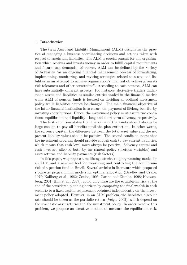
Table 1: Statistics, time series 1996Q2-2007Q2

The stochastic model for economic risk factors chosen is a Vector Auto-Regressive based on Dert (1998). The variables are chosen to model appro-priately the asset returns used as inputs for the optimization problem. Themean vector is specified exogenously and can be interpreted as a sensitivityparameter for the model response to the economic risk factors. This modelhas quarterly data with a sample representing the Brazilian economy from1996Q2 to 2007Q2.

Xq − � = �(Xq−1 − �) + �q, �q ∼ N(0,Σ) (8)

xj,q = log(1 + yjq), ∀j = 1, . . . , 5 (9)

Where

yj,q =

⎧

⎨

⎩

output growtℎ rate, j = 1

rental growtℎ rate, j = 2

inflation rate, j = 3

interest rate, j = 4

stock return, j = 5

The time series statistics are described in Table 1. As we see, the his-torical mean of Brazilian interest rate is too high because of some inter-national crisis (Asia-1997 and Russia-1998) and the hyperinflation processremnants at the beginning of the sample. For this reason, the mean ofthe economic variables must be determined exogenously, for example: � =(4%, 11%, 4%, 10%, 12%)′.

The other coefficients (Σ and �) are estimated using the Ordinary LeastSquares method, and are given by Tables 2 and 3.

7

x1 x2 x3 x4 x5

x1 0.001886 0.000347 0.000881 -0.000285 0.000084x2 0.000347 0.001927 0.001555 -0.000020 0.000123x3 0.000881 0.001555 0.008173 -0.000026 0.003296x4 -0.000285 -0.000020 -0.000026 0.000683 -0.000531x5 0.000084 0.000123 0.003296 -0.000531 0.036031

Table 2: Covariance matrix, quarterly 1996Q2-2007Q2

x1,q−1 − 0.04 x2,q−1 − 0.11 x3,q−1 − 0.04 x4,q−1 − 0.10 x5,q−1 − 0.12

x1,q − 0.04 -0.148696 -0.185559 -0.045314 -0.229618 0.086285(0.15288) (0.13395) (0.07164) (0.17779) (0.03676)

x2,q − 0.11 -0.422790 0.114880 0.064160 -0.919097 0.030370(0.15454) (0.13541) (0.07242) (0.17972) (0.03716)

x3,q − 0.04 0.040368 -0.176425 0.418518 0.176557 -0.174167(0.31828) (0.27888) (0.14915) (0.37014) (0.07654)

x4,q − 0.10 -0.008872 -0.078176 0.067767 0.657944 -0.088930(0.09198) (0.08059) (0.04310) (0.10697) (0.02212)

x5,q − 0.12 -0.431145 0.612786 -0.139294 0.066837 0.140459(0.66828) (0.58556) (0.31317) (0.77717) (0.16070)

Table 3: � coefficient, standard deviation in ( ), sample: 1996Q2-2007Q2

4. Scenario tree generation method

The scenario tree generation method is based on the “Adjusted RandomSampling” of Kouwenberg (2001). Some modifications were introduced inorder to take into account the different time intervals between nodes in ourevent tree. We modify the notation of the equation (8) to make the cor-respondence between the stage t of the event tree and the quarter q of thestochastic model. So, X t

q is the risk factor vector of q quarters ahead staget. The stochastic model is rewritten as (10).

X tq − � = �(X t

q−1 − �) + "tq, "tq N (0,Σ) (10)

The first step of the method is to generate a deterministic one-quarterforecast from the beginning of stage t for each predecessor node.

X tq − � = �

(

X tq−1 − �

)

(11)

The first (Nt −Nt−1) /2 values of "tq ∼ N (0,Σ) are randomly generated:

"tq (nt)N (0,Σ) , ∀nt = Nt−1 + 1, . . . , Nt/2 (12)

In order to guarantee the mean and the other odd central moments aszero, as stated by the Normal distribution, we take the antithetic values.

8

"tq (nt +Nt/2) = −"tq (nt) , ∀nt = Nt−1 + 1, . . . , Nt/2 (13)

Another adjustment is made in order to fit the variances of the tree struc-ture and the stochastic model. This adjustment is made for each component

j of the vector "tq (nt) =(

"t1,q (nt) , . . . , "t5,q (nt)

)′

.

�tj,q (nt) =�j

√

1Nt−1

∑Nt

i=1

(

"tj,q (nt))2"tj,q (nt) , ∀nt = Nt−1 + 1, . . . , Nt (14)

This process is repeated for all quarters of stage t computing Nt − Nt−1

independent scenarios. The last observation of each scenario belonging tostage t will initialize a set of conditional branches of stage t+1 restarting allover the process. Considering Q(t) the number of quarters that compoundstage t, the initialization for a given predecessor node nt is represented asfollows:

X t+10 = X t

Q(t) (nt) (15)

5. Asset pricing model

The asset pricing is an important part of ALM process. It consists oftransforming the economic risk factors into the asset class returns. Thestock return (16) is modeled as the return of stock index, the propertiesreturn (17) is modeled as the return on the rental activity, the bonds return(18) is the short term interest rate plus a deterministic spread and, finallythe cash return is the short term interest rate (19). Consider a pair of linkednodes (nt, nt−1), the returns are given as follows:

r1 (nt) =stock index (nt)

stock index (nt−1)− 1 (16)

r2 (nt) =rental activity (nt)

rental activity (nt−1)− 1 (17)

r3 (nt) = interest rate (nt) + spread (18)

r3 (nt) = interest rate (nt) (19)

9

Following (16), (17), (18) and (19) the asset returns are calculated asfunctions of economic risk factors. Since the economic factors are represented

as components of the vector ytq (nt) =(

yt1,q (nt) , . . . , yt5,q (nt)

)′

and xj,q (nt) =

ln(

1 + ytjq (nt))

, ∀j = 1, . . . , 5, the returns of each node are computed asfollows:

r1 (nt) = exp

⎛

⎝

1

Q (t)

Q(t)∑

q=1

xt5,q (nt)

⎞

⎠− 1 (20)

r2 (nt) = exp

⎛

⎝

1

Q (t)

Q(t)∑

q=1

xt2,q (nt)

⎞

⎠− 1 (21)

r3 (nt) =

⎡

⎣exp

⎛

⎝

1

Q (t)

Q(t)∑

q=1

xt4,q (nt)

⎞

⎠− 1

⎤

⎦+ spread (22)

r4 (nt) = exp

⎛

⎝

1

Q (t)

Q(t)∑

q=1

xt4,q (nt)

⎞

⎠− 1 (23)

6. Liability model

We created an artificial data base of a pension fund with 110200 partic-ipants distributed as 45000 active, 60000 retired 5200 pensioners. All theparticipants have a defined benefit plan to which they contribute, along withthe plan sponsor, 16% of their salary to receive a benefit of 90% of the lastsalary after retirement. Let Ideatℎ be a dummy variable assuming 1 whenthe participant is dead and 0 otherwise. Similarly Iret assumes 1 when theparticipant is retired and 0 otherwise. Thus, the contribution of participantp at year k is defined in (24) while the benefit of participant p at year k isdefined in (25).

contribution (p, k) = 0.16salary (p, k) (1− Ideatℎ) (1− Iret) (24)

benefit (p, k) = 0.9last salary (p, k) (1− Ideatℎ) Iret (25)

Considering a deterministic age of retirement, the expected contribu-tion and benefit of participant p at year k are defined, respectively, in (26)

10

and(27). The expected values are used due to the large number of partici-pants and the independence assumption over their time of death.

E [contribution (p, k)] = 0.16 ⋅ salary (p, k) ⋅(

1− qage(p))

⋅ (1− Iret) (26)

E [benefit (p, k)] = 0.9 ⋅ last salary (p, k) ⋅ (1− qdeatℎ) ⋅ Iret (27)

The expected values are accumulated for all participants in (28).

RF (k) =10200∑

p=1

{E [benefit (p, k)]− E [contribution (p, k)]} (28)

7. Equilibrium risk measuring method

The equilibrium risk is defined as the insolvency probability, i.e., the prob-ability that the pension fund won’t meet all obligations until its extinction.In other words, insolvency is a state at a defined instant of time where thetotal asset value is smaller than the net present value of the fund’s liabilities,namely the technical reserve.

The total asset value at a determined instant of time is easily calculatedby the sum of the amount invested in each asset class. On the other hand,the technical reserve calculation is more complicated because the net presentvalue of the fund’s liability cash flows needs a discount rate which, followingVeiga (2003), should be the fund’s portfolio return. In the first years un-der study, this calculation is implicitly done by the stochastic optimizationmodel. However, the liability horizon is, usually, longer than the period cho-sen to optimize the investment policy. Thus, the portfolio return for eachscenario, given the optimal decisions, is known only for these first years whilesome assumptions are needed to model the remaining period.

Choosing a fixed discount rate is not necessarily a good approximationfor the portfolio returns of this remaining period nonetheless the previouspapers in the literature have assumed this approach for mostly based on aregulatory statement of the country under study. Thus, their approximationgives rise to an arbitrary technical reserve and, consequently, a meaninglessequilibrium risk measure.

In order to solve this inadequacy, we propose a new method to betterestimate the equilibrium risk. First an optimal solution is obtained with

11

�

�

��

��

��

��

��

��

��

��

�

�

�

� � � � ��

�

��

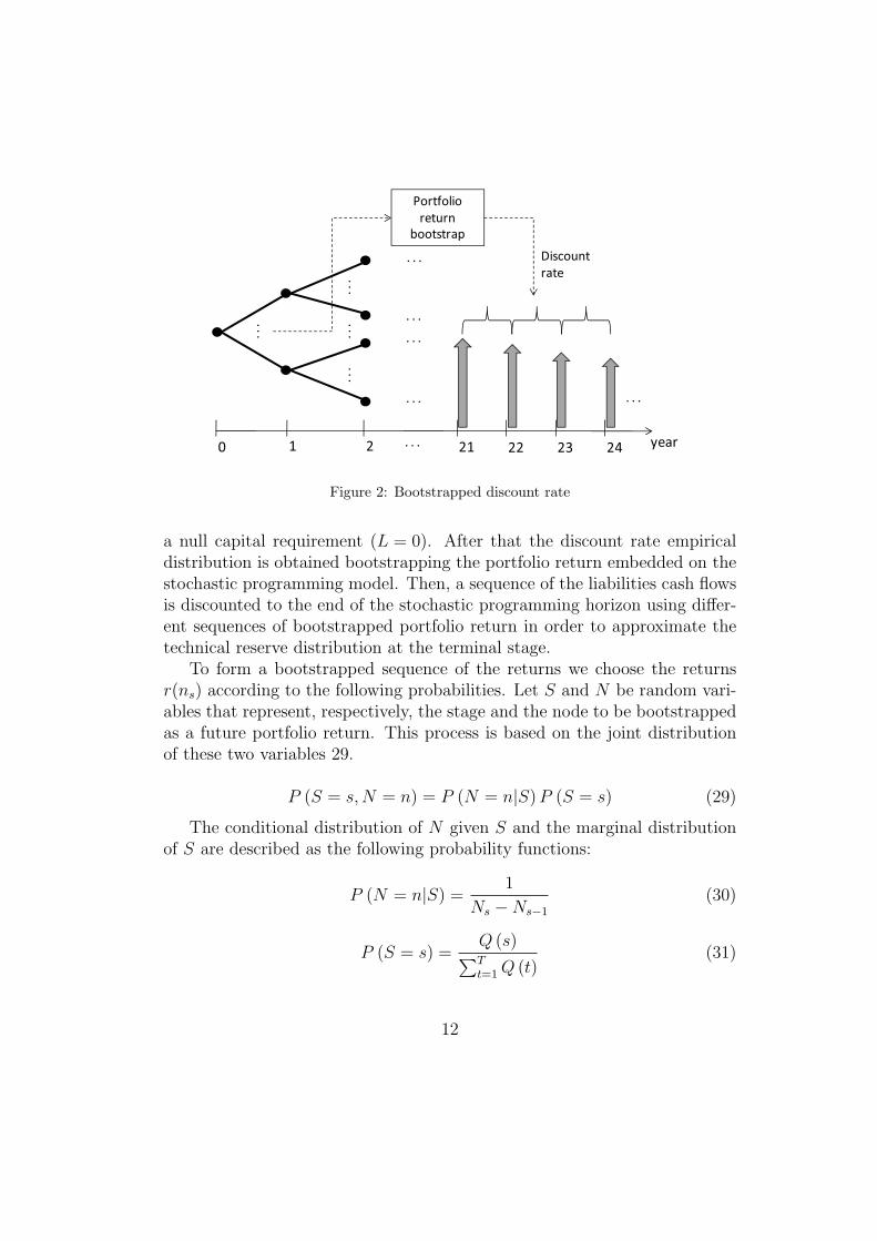
Figure 2: Bootstrapped discount rate

a null capital requirement (L = 0). After that the discount rate empiricaldistribution is obtained bootstrapping the portfolio return embedded on thestochastic programming model. Then, a sequence of the liabilities cash flowsis discounted to the end of the stochastic programming horizon using differ-ent sequences of bootstrapped portfolio return in order to approximate thetechnical reserve distribution at the terminal stage.

To form a bootstrapped sequence of the returns we choose the returnsr(ns) according to the following probabilities. Let S and N be random vari-ables that represent, respectively, the stage and the node to be bootstrappedas a future portfolio return. This process is based on the joint distributionof these two variables 29.

P (S = s,N = n) = P (N = n∣S)P (S = s) (29)

The conditional distribution of N given S and the marginal distributionof S are described as the following probability functions:

P (N = n∣S) =1

Ns −Ns−1

(30)

P (S = s) =Q (s)

∑T

t=1Q (t)(31)

12

��

��

��

��

��

��

��

��

��

��

��

��

��

��

��

��

�

��

��

��

��

��

��

� ��

��

��

��

Figure 3: Equilibrium risk measure

Using the stochastic discount rate, the technical reserve distribution canbe estimated and consequently a conditional insolvency probability is calcu-lated for each terminal node of the tree structure. Indeed, the conditionalinsolvency probability is calculated as the maximum p-value which the tech-nical reserve is greater than the wealth of each terminal node. Finally, theinsolvency probability at the root node will be the average of all a conditionalinsolvency probabilities since all scenarios have the same probability.

To sum up, the insolvency probability has to be compared to the fund’srisk tolerance to accept the optimal solution. If the equilibrium risk is onan acceptable level then the optimal allocation is defined. But if the equi-librium risk is too high, there are two possibilities to decrease the insolvencyprobability without changing the initial wealth: raising the insolvency pe-nalization or changing the capital requirement (L) from zero to one quantileof the technical reserve distribution. To test the possible equilibrium riskcontrol we implemented the latter iterative method.

13

��

��

��

��

��

��

��

��

Underfunding and Insolvency Probabilities

��

��

��

��

��

��

��

��

��

Figure 4: Underfunding and Insolvency probability

8. Illustrative example

The illustrative example has the objective of comparing two non-arbitraryequilibrium risk measures: the underfunding probability and the insolvencyprobability. An underfunding state is defined as a negative wealth at theend of the stochastic programming horizon while the insolvency state is de-scribed by a deficit at the end of the fund existence. Since the stochasticprogramming horizon is smaller than the fun existence, the underfundingprobability is a lower bound for the insolvency probability, underestimatingthe actual equilibrium risk. The underfunding probability will be calculatedas a proportion of the scenarios negative terminal wealth and the insolvencyprobability will be calculated with the bootstrap method proposed in thispaper. Furthermore, the iterative method which increases the capital re-quirement (L) will also be tested.

First, it is proposed to run the whole process with different initial wealthconsidering a null capital requirement (Figure 4). This example confirmsthe theoretical result that the underfunding probability underestimates theactual equilibrium risk, the insolvency probability.

Second, it is proposed, for several different initial wealth, an influential

14

analysis of capital requirement on the insolvency probability. Four cases areconsidered:

∙ Case 1: Null capital requirement

∙ Case 2: Iterative method

– Step 1: Null Capital requirement

– Step 2: Capital requirement as the average technical reserve

∙ Case 3: Iterative method

– Step 1: Null Capital requirement

– Step 2: Capital requirement as the reserve with risk correction(1% significance)

∙ Case 4: Capital requirement as a predetermined value (real discountrate: 6% by Brazilian law)

It is confirmed that when the capital requirement is increased the insolvencyprobability is decreased. Figure 5 also shows that the differences betweeneach case are small suggesting that the main factor that influences the equi-librium risk is the initial wealth.

9. Conclusions

This paper proposed an ALM multistage stochastic programming modelfor a Brazilian pension fund and a new methodology of measuring and con-trolling the equilibrium risk. To do this, the whole process was divided intosmall parts and each one was described in details. A flowchart (Figure 6)can summarize the whole process.

The process begins with the estimation of the stochastic model coeffi-cients used to generate the risk factor tree structured scenarios. So, financialmodels are used to do the asset pricing and the liability cash flow calcula-tion. After that, the asset returns and the liability cash flows are used as thestochastic programming inputs to find an optimal investment policy with nullcapital requirement. Then, the optimal portfolio returns are bootstrappedto obtain the technical reserve distribution. Finally, using this result, the

15

��

��

��

��

��

��

��

��

��

��

��

��

��

��

��

��

� ��

Figure 5: Insolvency probability

��

��

��

��

��

��

��

��

��

��

��

Stochastic model

Scenario Tree

Generation

AssetPricing

Optimization

BootstrapReturnsinflation

Risk Measure

��

��

��

��

��

��

��

!� ��"��

# ��

��

Optimization Model

Measure

Risk Acceptance

Liability Model

Figure 6: Flowchart

16

insolvency probability is estimated as the average of the conditional insol-vency probabilities calculated for each terminal node. If the risk acceptancecriteria is satisfied, then the optimal allocation is defined, else another so-lution is obtained with a higher capital requirement or a higher insolvencypenalization.

In conclusion, this proposed methodology can give a better estimate ofthe equilibrium risk involved in a pension fund. In fact, the underfundingprobability (previous work non-arbitrary risk measure) underestimates thelong term risk of a pension fund since it is much smaller than the insolvencyprobability. Moreover, it was also tested an iterative method, increasing thecapital requirement, to control the equilibrium risk. For instance, on theillustrative example, this approach actually decreased the insolvency proba-bility however it shows just small improvements controlling the equilibriumrisk.

References

Bradley, S. P., Crane, D. B., Oct. 1972. A dynamic model for bond portfoliomanagement. Management Science 19 (2), 139–151.

Carino, D. R., Ziemba, W. T., Jul. 1998. Formulation of the Russell-Yasudakasai financial planning model. Operations Research 46 (4), 433–449.

Dert, C. L., 1998. A dynamic model for asset liability management for de-fined benefit pension funds. In: Worldwide asset and liability modeling,william t. ziemba, john m. mulvey Edition. Cambridge University Press,Cambridge, UK, pp. 501–536.

Hilli, P., Koivu, M., Pennanen, T., Ranne, A., Jul. 2007. A stochastic pro-gramming model for asset liability management of a finnish pension com-pany. Annals of Operations Research 152 (1), 115–139.

Kallberg, J. G., White, R. W., Ziemba, W. T., Jun. 1982. Short term financialplanning under uncertainty. Management Science 28 (6), 670–682.

Kouwenberg, R., Oct. 2001. Scenario generation and stochastic programmingmodels for asset liability management. European Journal of OperationalResearch 134 (2), 279–292.

17

Veiga, A., 2003. Medidas de risco de equilibrio em fundos de pensao. In:Gestao de Riscos no Brasil, antonio m. duarte jr., gyorgy vargas. Edition.Vol. 1. Editora Financial Consultoria, Rio de Janeiro, pp. 645–666.

Zenios, S., Dec. 1995. Asset/liability management under uncertainty forfixed-income securities. Annals of Operations Research 59 (1), 77–97.

18

On the Asset and Liability Management for pension funds: a ...

Documents

Transcript of On the Asset and Liability Management for pension funds: a ...