On the Annual Variations in the Amplitude of 25-70-Day...

Earth Sciences 2016; 5(3): 39-47

http://www.sciencepublishinggroup.com/j/earth

doi: 10.11648/j.earth.20160503.11

ISSN: 2328-5974 (Print); ISSN: 2328-5982 (Online)

On the Annual Variations in the Amplitude of 25-70-Day Intraseasonal Atmospheric Oscillations in Central Africa

Alain Tchakoutio Sandjon1, 2, 3, *

, Armand Nzeukou2

1Department of Computer Science, Higher Technical Teachers Training College (HTTTC), University of Buea, Kumba, Cameroon 2Laboratory of Industrial Systems and Environmental Engineering, Fotso Victor Technology Institute, University of Dschang, Bandjoun,

Cameroon 3Laboratory for Environmental Modeling and Atmospheric Physics, Department of Physics, Faculty of Sciences, University of Yaoundé 1,

Yaoundé, Cameroon

Email address: [email protected] (A. T. Sandjon), [email protected] (A. T. Sandjon) *Corresponding author

To cite this article: Alain Tchakoutio Sandjon, Armand Nzeukou. On the Annual Variations in the Amplitude of 25-70-Day Intraseasonal Atmospheric

Oscillations in Central Africa. Earth Sciences. Vol. 5, No. 3, 2016, pp. 39-47. doi: 10.11648/j.earth.20160503.11

Received: May 25, 2016; Accepted: July 13, 2016; Published: July 23, 2016

Abstract: In this paper we analyzed the annual variations in the 25-70-day intraseasonal atmospheric oscillations in

central Africa, for the period 1981-2010, using the Outgoing Longwave OLR data. We then extracted the amplitude time

series of the dominant modes of intraseasonal variability in 25-70 days filtered OLR anomalies, using Empirical Orthogonal

Functions (EOF) analysis. The EOF analysis has shown that three dominant modes characterized the intraseasonal

atmospheric oscillation in Central Africa. The amount of variance explained by these three retained EOFs are 19.3%, 13.6%

and 11.8% respectively, and they exhibit higher spatial loading over Northern Congo, Southern Ethiopia, and Southwestern

Tanzania, respectively. The analysis of Principal Components (PCs) time series showed that the amplitude and of the

intraseasonal oscillations (ISO) exhibit large annual variations. In fact the highest values of ISO amplitude are generally

observed during October-April season, and much weakened signal the rest of the year. The fraction of yearly Madden Julian

Oscillation (MJO) power, occurring within October-April season are 79.3%, 77.92%, 78.73% for EOF1, EOF2, and EOF3,

respectively.

Keywords: Rainfall, ISO Variations, Central Africa, Amplitude

1. Introduction

It is well-known that climate variability and change is a

crucial problem in many tropical regions. Amongst these

regions, the central Africa (CA) is particularly attractive

interesting because of the variety of its topography and

surface conditions. The CA extends from 15°S to 15°N and

5-45°E mainly over the land and part of Atlantic and Indian

oceans on its edges. The topography of the region includes

Highlands, mountains, Plateaus (Fig. 1a). Furthermore, CA is

particularly vulnerable because the majority of its population

is rural and practice rainfed agriculture. Then high frequency

climate variability, from daily to intraseasonal timescales is a

significant source of vulnerability in the region.

The western part (15°S-15°N; 5-30°E) of CA is

consisting of the zones of intense precipitation, especially

over the Congo Basin (Fig. 1b). In fact, the western central

Africa is almost covered by the Congo forest, which keeps

this region quite wet within the year. The Eastern part

(15°S-15°N; 30-50°E) is characterized by widely diverse

climates ranging from desert to forest over relatively small

areas. The complex topography of the region is an

important contributing factor to climate because it leads to

the orographically induced rainfall and affect local climates

[1, 2]. This region has suffered from both excessive and

deficient rainfall in recent years [3, 4]. In particular, the

frequency of anomalously strong rainfall causing floods has

increased. The difference between the East and West

boundaries of CA of approximately 3000m in surface

elevation, and 3000mm in annual mean rainfall. Then the

40 Alain Tchakoutio Sandjon and Armand Nzeukou: On the Annual Variations in the Amplitude of 25-70-Day

Intraseasonal Atmospheric Oscillations in Central Africa

two subregions (ECA and WCA), separated from each other

by the Rift Valley, are very different in term of topography,

surface conditions and precipitation (Table 1).

Table 1. Comparison of some geographical features between eastern and western central Africa.

Western Central Africa (WCA) Eastern Central Africa (ECA)

Average topography Lower than 700m Greater than 1500m

Vegetation Almost covered by the Congo forest From desert to minor forests over relatively small areas

Mean annual rainfall Greater then 1600mm Lower than 700mm

Borders Rift Valley-Atlantic ocean Rift Valley-Indian ocean

Fig. 1. (a) Surface elevation over the study area based on 30-min topographic data (m) from Digital Elevation Model (DEM) of the US Geological Survey. The

study domain (15oS-15oN 5-45oE) is shown as solid box. (b) Annual mean rainfall (in mm), based from 1DD GPCP data.

The Inter-Tropical Convergence Zone (ITCZ) is a classical

and dominant feature of atmospheric dynamics over the

region [5, 6]. Then the rainfall over CA is highly seasonal.

The peak of ITCZ precipitation belt shifts from north to south

of the equator during November-December and returns to

north during March-April. The ITCZ precipitation maximizes

near 10°N during summer, while it peaks near 10°S during

winter. Around the equator (6°S-6°N), the mean annual

rainfall is divided into four periods or seasons: December-

February (DJF), March-May (MAM), June-August (JJA),

and September-November (SON).

The Madden-Julian Oscillation (MJO) is an intraseasonal

fluctuation occurring in the global tropics. It was shown in

many studies that MJO is the dominant mechanism of tropical

variability at intraseasonal timescales [7, 8, 9, 10, 11, 12, 13],

and results in variations in several important atmospheric and

oceanic parameters which include both lower- and upper-level

wind. The MJO is characterized by eastward propagation of

regions of enhanced and suppressed tropical rainfall, primarily

over the Indian and Pacific Oceans. The anomalous rainfall is

often first evident over the Indian Ocean, and remains apparent

as it propagates eastward over the very warm water of the

western and central tropical Pacific.

An important characteristic of the MJO (ISO) is its

irregularity within the year, and from year to year. In fact the

modulation of the level of MJO activity and its possible

predictability is one of the greatest challenges and it has been

the key subject of many researches (e.g. [14, 15, 16, 17]).

However almost all studies on the variations of MJO activity

focused on the interannual variations of the signal. For year-

to-year variability in MJO activity, many authors found

strong interannual modulation of MJO activity, with periods

of strong activity followed by periods in which the oscillation

is weak or absent [18, 19]. For example in Central Africa,

[17] studied the interannual modulation of ISO activity in

Central Africa and the relationships with El Nino Southern

Oscillation (ENSO) It is also known that MJO activity

exhibits annual variations. For example, here are strong

annual variations in the MJO activity, with some months with

high intensity signal and other months with low intensity

signal. Unfortunately, almost no study has been carried out in

Central Africa concerning the variations of ISO activity

within the year. The question is addressed in this paper. Some

mathematical tools are used to assess the variations patterns

of the amplitude of the intraseasonal oscillations in CA

within the year.

The paper is organized as follows: In the next section, the

data and methods used will be described. Section 3 will

present the main results obtained and the analyses. Finally,

Section 4 is devoted to a few discussions and conclusions.

Earth Sciences 2016; 5(3): 39-47 41

2. Data and Methods

2.1. Data Used

In this study, the Outgoing Longwave Radiation (OLR) is

used as a rainfall proxy. Since 1974, launching polar orbital

National Oceanic and Atmospheric Administration (NOAA)

and Television Infrared Observation Satellite (TIROS)

satellites has made it possible to establish a quasi-complete

series of twice-daily measures of outgoing longwave

radiation (OLR), at the top of the atmosphere and at a spatial

resolution of 2.5° latitude–longitude [20]. The interpolated

OLR dataset [21] provided by the Climate Diagnostics

Center has been used here. In tropical areas, deep convection

and rainfall can be estimated through low OLR values. Local

hours of the measures varied during the period 1979–1990

between 0230 and 0730 in the morning time and between

1430 and 1930 in the afternoon time. Since the deep

convection over Central Africa has a strong diurnal cycle [2],

the sample of daily OLR based on two values separated by

12h is enough to get a daily average. In the tropics where

surface temperatures varies modestly trough the annual cycle,

the strongest variation in the OLR result from changes in the

amount and depth of clouds. This direct physical connection

with clouds led to the use of OLR in quantitative

precipitation estimation [2, 22, 23]. This product is available

on the NOAA website http://www.esrl.noaa.gov and can be

freely downloaded.

The Niño-3.4 region (5°S–5°N, 160°E–150°W) sea surface

temperature anomaly (SSTA)index was also used, to define

the strength of ENSO and identify individual El Niño and La

Niña events [24] These Monthly observed SSTA are adapted

from the National Oceanic and Atmospheric Administration

(NOAA Climate Diagnostics Center).

2.2. Methods

Depending on the purpose of analysis, some frequencies

may be of greater interest than others, and it may be helpful

to reduce the amplitude of variations at other frequencies by

statistically filtering them out before viewing and analyzing

the series. The Lanczos filtering [25] used in this study is one

of the Fourier methods of filtering digital data. Its principal

feature is the reduction of the amplitudes of Gibbs

oscillation. The Fourier coefficients for the smoothed

response function are determined by multiplying the original

weight function wk, by a function that Lanczos called “sigma

factors”. Then the weight function of relation becomes [26]:

nk

nk

k

kfw c

k/

/sin.

2sin

ππ

ππ

= (1)

where k

kfw c

k ππ2sin= are the traditional Fourier weights.

The Lanczos filter is widely used for filtering climate data

time series.

Commonly, some form of time series or spectral analysis is

used for extracting periodic signatures from a set of data

pertaining to climate variations. Fourier series provides an

alternate way of representing data: instead of representing the

signal amplitude as a function of time, we represent the

signal by how much information is contained at different

frequencies. A Fourier series takes a signal and decomposes it

into a sum of sines and cosines of different frequencies.

∑+∞

=

++=1

0 )2sin()2cos()(n

nn ntbntaatf ππ (2)

Where f(t) is the signal in the time domain, and an and bn

are unknown coefficients of the series, which can be found

by simple integration. In atmospheric sciences, we generally

work with discrete data points, not an analytical function that

we can analytically integrate. It turns out that taking a

Fourier transform of discrete data is done by simply taking a

discrete approximation to the integrals. Inversely, the Fourier

Transform generates values of amplitudes and phases

averaged over the entire time series for each frequency

component or harmonic. The amplitude of signal can then be

represented as a frequency, and the dominant frequencies are

highlighted.

The Wavelet Analysis (WA) is a time series analysis

method that has increasingly been applied in geophysics

during the last three decades. It is becoming a common tool

for analyzing temporal variations of power within a time

series. The transformation in time series from the time

space into the time-frequency space show that, the WA is

able to determine both the dominant timescales of

variability and how they vary with time. WA has several

attractive advantages over the traditional spectral analysis,

especially when dealing with time series with time-varying

amplitudes. In contrast to the Fourier Transform, that

generates values of amplitudes and phases averaged over

the entire time series for each frequency component or

harmonic, Wavelet Transform provides a localized

instantaneous estimate of the amplitude and phase for each

spectral component of the series. This gives WA an

advantage in the analysis of non-stationary data in which

the amplitude and phase of the harmonic components may

change rapidly in time or space. While the Fourier

Transform of the non-stationary time series would smear

out any detailed information on the changing features, the

WA keeps track of the evolution of the signal characteristics

throughout the time series. Further details on wavelet

analysis can be found in [28].

In the last several decades, meteorologists have in fact put

major efforts in extracting important patterns from

measurements of atmospheric variables. As a result Empirical

Orthogonal Functions (EOF) technique has become the most

widely used way to do this [9].

The original purpose of EOFs was to reduce the large

number of variables of the original data to a few variables,

but without compromising much of the explained variance.

Lately, however, EOF analysis has been used to extract

individual modes of variability (eg. [7, 9, 13, 17, 28, 29]) in

data time series. In the EOF analysis, the time-dependent



deviations from the long-term mean are decomposed into a

sum of products of fixed spatial patterns pk and time-

dependent amplitudes k

αααα (the principal components) as

follows:

)()(),( txptxf kiki α∑= (3)

Where the principal components kα are uncorrelated to

one another and described subsequently a maximum of

variance in the original anomalies field f. Under these

conditions the EOFs pk are eigenvectors of the covariance

matrix of f.

The eigen value λk corresponding to the kth

EOF gives a

measure of the explained variance by k

αααα . It is usual to write

the explained variance in percentage as:

∑=

p

i

i

k

1

.100

λ

λ% (4)

Rotated EOF (REOF) is a technique simply based on

rotating EOFs. REOF techniques have been adopted by

atmospheric scientists since the mid-eighties as an attempt to

overcome some of the previous short comings such as the

difficulty of physical interpretability. The technique,

however, is much older and goes back to the early forties.

The technique is also known in factor analysis as factor

rotation and aims at getting simple structures. In

meteorology, he objective was to alleviate the strong

constraints of EOFs, namely orthogonality/ uncorrelation of

EOFs/PCs, domain dependence of EOF patterns (see e.g.,

Dommenget and Latif, 2002), obtain simple structures, and

be able to physically interpret the patterns. Initially, a

standard EOF analysis is performed and an EOF subset is

retained; and subjected to varimax rotation. Some think that

the resulting patterns are more physically interpretable. The

patterns may still be domain dependent.

The above described mathematical tools (Lanczos

filtering, Fourier analysis, wavelet analysis and EOFs

analysis) are simultaneously used in this paper. Briefly the

long-term OLR anomalies are firstly passed through the high-

pass Lanczos filter with 120 days cut off in order to remove

low frequencies modes such as inter-seasonal and interannual

variability. Morlet wavelet is applied to the output time series

to extract the relevant information. After the wavelet

analysis, the timescales where the intraseasonal signal power

is relatively high are detected. The original time series are

now passed through a band-pass Lanczos filter to retain only

the cycles with periods within the relevant timescales. The

filtered data-sets then have been subjected to EOF analysis

with varimax rotation and the leadings PCs are retained

according to the Scree test [31] and the North criteria [32].

After the PCs time series have been extracted, the variations

in the ISO magnitude and was studied using statistical

methods.

3. Results and Analyses

3.1. Spectral Analysis

For every day and each of the two datasets, we averaged the

120 days cut-off high-pass filtered OLR values, of all grid

points in the study area to have a mean value. The classical

Fourier analysis was then performed on the obtained daily time

series. The power spectrum of this time series (Fig. 2) reveals

the importance of the intraseasonal variability present in the

Central African climate. At intraseasonal time scales, the

strongest peaks of convective variability are centered near 50

days and extended over the longer periods (20–80days,

corresponding to the frequencies of 0.0125–0.05day−1

).

Fig. 2. Calculated spectrum (solid black line), red noise curve (green solid

line) and the curves indicating the upper (red dashed line) and lower (blue

dashed line) confidence bounds for the period 1981-2010, using OLR data.

Fig. 3. Annual mean wavelet power spectrum of the rainfall anomalies

averaged over CA. A 120-day cut off low-pass filter was applied to long-

term anomalies in order to remove low-frequency modes such as inter-

seasonal and interannual variability.

As stated in the previous section, wavelet analysis is an

attractive tool for analyzing temporal variations of power

within a time series because it keeps track of the evolution of

the signal characteristics throughout the time series. Figure 4

shows the wavelet spectrum for the OLR data, obtained from

the wavelet analysis applied on the averaged time series

described above, and following the technique described by

[27]. To show how the signal varies throughout the year, the

Earth Sciences 2016; 5(3): 39-47 43

wavelet power was computed on the entire time series (1981–

2010), and the daily climatology was calculated at each

frequency, to plot the annual cycle (Fig. 3). It clearly appears

that, high wavelet powers are much concentrated at

intraseasonal timescales (20–80 days), in consistency with the

classical Fourier analysis of Fig. 2. The seasonality of

intraseasonal oscillations is clearly defined, since the

maximum power during the beginning and end of the year

(October–April) and much weakened or no signal during

June–September period. This seasonality can be explained by

the location of the study area along the equator [35]. A

frequency band of the highest wavelet powers is highlighted in

the plot. This band is centered near a period of 50 days. This

result confirms that the dominant component of intraseasonal

atmospheric variability in Central Africa is MJO [30].

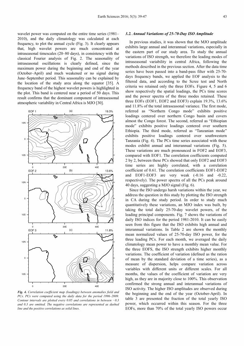
Fig. 4. Correlation coefficient map (loadings) between anomalies field and

PCs. PCs were computed using the daily data for the period 1996–2009.

Contour intervals are plotted every 0.05 and correlations in between −0.3

and 0.3 are omitted. The negative correlations are represented as dashed

line and the positive correlations as solid lines.

3.2. Annual Variations of 25-70-Day ISO Amplitude

In previous studies, it was shown that the MJO amplitude

exhibits large annual and interannual variations, especially in

the eastern part of our study area. To study the annual

variations of ISO strength, we therefore the leading modes of

intraseasonal variability in central Africa, following the

methods described in the previous section. After the data time

series have been passed into a band-pass filter with 25-70-

days frequency bands, we applied the EOF analysis to the

filtered data, and according to the Scree test and North

criteria we retained only the three EOFs. Figure 4, 5 and 6

show respectively the spatial loadings, the PCs time scores

and the power spectra of the three modes retained. These

three EOFs (EOF1, EOF2 and EOF3) explain 19.3%, 13.6%

and 11.8% of the total intraseasonal variance. The first mode,

referred as “Northern Congo mode” exhibits positive

loadings centered over northern Congo basin and covers

almost the Congo forest. The second, referred as “Ethiopian

mode” exhibits positive loadings centered over southern

Ethiopia. The third mode, referred as “Tanzanian mode”

exhibits positive loadings centered over southwestern

Tanzania (Fig. 4). The PCs time series associated with these

modes exhibit annual and interannual variations (Fig. 5).

These variations are much pronounced in FOF2 and EOF3,

compared with EOF1. The correlation coefficients computed

2 by 2, between these PCs showed that only EOF2 and EOF3

time series are highly correlated, with a correlation

coefficient of 0.61. The correlation coefficients EOF1-EOF2

and EOF1-EOF3 are very weak (-0.16 and -0.22,

respectively). The power spectra of all the PCs peak around

40 days, suggesting a MJO signal (Fig. 6).

Since the ISO undergo harsh variations within the year, we

address the question in this study by plotting the ISO strength

in CA during the study period. In order to study much

quantitatively these variations, an MJO index was built, by

taking the total daily 25-70-day wavelet powers, of the

leading principal components. Fig. 7 shows the variations of

daily ISO indices for the period 1981-2010. It can be easily

seen from this figure that the ISO exhibits high annual and

interannual variations. In Table 2 are shown the monthly

mean normalized values of 25-70-day ISO power, for the

three leading PCs. For each month, we averaged the daily

climatology mean power to have a monthly mean value. For

the three EOFS, the ISO strength exhibits higher monthly

variations. The coefficient of variation (defined as the ration

of mean by the standard deviation of a time series), as a

measure of dispersion, helps compare variation across

variables with different units or different scales. For all

months, the values of the coefficient of variation are very

high, as they are in majority close to 100%. This observation

confirmed the strong annual and interannual variations of

ISO activity. The higher ISO amplitudes are observed during

the beginning and the end of the year (October-April). In

table 3 are presented the fraction of the total yearly ISO

power, which occurred within this season. For the three

EOFs, more than 70% of the total yearly ISO powers occur



during October-April (79.73%, 77.92%, and 78.3% for

EOF1, EOF2 and EOF3, respectively).

Fig. 5. Time series of the amplitude of the three leading PCs. The EOFs

analysis was performed on the entire period (1981–2010). The amplitudes

are in W.m-2 and the plot formats are identical.

Fig. 6. Power spectra of PC1 (bold solid), PC2 (thin solid), and PC3 (thin

dashed), respectively. The scale of the x- axis is in days and the power

dimensionless because the anomalies field is normalized.

Table 2. Monthly statistical values (mean, standard deviation, coefficient of

variation) of ISO power, for the three leading PCs.

EOF1 EOF2 EOF3 Mean Standard

deviation

Coefficient

of Variation

Jan 0.62 0.50 0.44 0.52 0.39 0.90

Feb 0.67 0.54 0.47 0.58 0.43 0.92

Mar 0.65 0.59 0.57 0.60 0.45 0.87

Apr 0.47 0.48 0.43 0.46 0.38 0.73

May 0.29 0.30 0.33 0.30 0.26 0.63

Jun 0.21 0.27 0.25 0.24 0.14 0.54

Jul 0.16 0.10 0.09 0.12 0.08 0.50

Aug 0.14 0.09 0.08 0.10 0.09 0.71

Sep 0.12 0.11 0.09 0.11 0.13 1.04

Oct 0.25 0.29 0.31 0.28 0.12 0.77

Nov 0.35 0.40 0.38 0.38 0.15 0.59

Dec 0.61 0.57 0.51 0.56 0.45 0.88

Table 3. Distribution of the total annual ISO power, for October-April and

May-September seasons.

EOF1 EOF2 EOF3

October-April 79.73% 77.92% 78.73%

May-September 20.27% 22.08% 21.27%

This seasonality of ISO is illustrated in the plots of figures

8 and 9. In figure 8, are represented the monthly mean

normalized ISO powers, and in figure 9 are plotted the

anomalies (deviation from the monthly mean). One may note

in figure 9 that the anomalies are almost positive during

October-April and negative during May-September. But this

seasonality is much pronounced in the Eastern part of the

region (EOF2 and EOF3). We also represented the

cumulative percentage mean power, as function of the day of

the year (Fig. 10). Once again, it can be seen that in the

eastern part of the region (EOF2 and EOF3), the ISO activity

is highly seasonal. For these two EOFs, this percentage

increases rapidly with time between 0-100 days, where

cumulative percentage mean power from these 3 months rises

from 0 to approximately 70% for EOF2 and EOF3 and only

62% for EOF1. This value remains roughly constant between

100-280 days (mid-October).

Fig. 7. Time series of MJO index within the period 1981-2010.

Fig. 8. Monthly variations of averaged power of 25-70-day intraseasonal

oscillations, deduced from the three leading PCs.

1985 1990 1995 2000 2005 2010−200

0

200

Am

plit

ud

e

EOF1

1985 1990 1995 2000 2005 2010−200

0

200

Am

plit

ud

e

EOF2

1985 1990 1995 2000 2005 2010−200

0

200

Years

Am

plit

ud

e

EOF3

1985 1990 1995 2000 2005 20100

0.5

1

1.5

ISO

in

dic

es

EOF1

1985 1990 1995 2000 2005 20100

0.5

1

1.5

2

2.5

ISO

in

dic

es

EOF2

1985 1990 1995 2000 2005 20100

0.5

1

1.5

2

Years

ISO

in

dic

es

EOF3

Jan Feb Mar Apr May Jun Jul Aug Sep Oct Nov Dec0

0.1

0.2

0.3

0.4

0.5

0.6

0.7

Months

Me

an

No

rma

lize

d in

dic

es

Earth Sciences 2016; 5(3): 39-47 45

Fig. 9. Monthly anomalies of the 25-70-day mean ISO power, for the three

leading PCs.

Fig. 10. Cumulated percentage mean ISO power for EOF1 (thin black),

EOF2 (black dashed), and EOF3 (gray).

To have more information about the onset and decay of

ISO activity, i.e. the period of the year corresponding to high

ISO strength, we introduced in this study an index called

Index of Variation of ISO Strength (IVS). The determination

of this index is based on the rate of the variations of ISO

power within two consecutive time intervals. Let’s consider P

(ti-1), P (ti) and P (ti+1), the ISO power at time steps ti-1, ti and

ti+1, respectively. The Index of Variation of ISO Strength

(IVS) for the ith

day is given by:

)()(

)()(

1

1

−

+

−−

=ii

ii

tPtP

tPtPIVS (5)

Then from the equation 4, an abrupt increase (resp.

decrease) of the IVS can be interpreted as the onset (resp.

decay) of ISO activity. A value of CVS close to one can be

interpreted as a permanent regime (high or low season),

while an abrupt change indicates a change in the ISO regime.

Figure 11 shows the evolution of IVS throughout the year. As

we could expect from Figure 10, the seasonality of ISO is not

clearly defined for EOF1, since the graph of variations of

IVS revealed many abrupt changes. But all this changes are

observed between 100-282 days. For EOF2 and EOF3, the

seasonality is clearly defined, as we can observe only 2

abrupt changes on the plots, corresponding to onset and

decay of ISO activity. The onset and decay dates for ISO

activity, as defined above, are shown in table 4. This table

confirmed that ISO activity exhibits higher amplitude during

October-April season.

Table 4. Average onset and retreat dates for ISO activity, using IVS.

Average onset date Average decay date

EOF1 Day 285 (12nd October) Day 99 (08th April)

EOF2 Day 279 (05th October) Day 92 (01st April)

EOF3 Day 273 (01st August) Day 94 (04th April)

Fig. 11. Evolution of the Index of Variation of ISO Strength (IVS) throughout

the year.

4. Summary and Conclusions

In this study, we examined the annual variations in the 25-

70-day intraseasonal oscillations of convective activity over

central Africa, using the daily Outgoing Longwave Radiation

datasets, for the period 1981-2010. A spectral analysis

indicates that the intraseasonal variability is dominated by

20–80 days periods band, with center near 40–50 days,

revealing that MJO could be the dominant component of

intraseasonal variability over CA during the last three

decades. A wavelet analysis also showed that intraseasonal

precipitation variability in CA is dominated 20-80 days

timescales with significant spectral peaks centered around

period of 40 days, in consistency with the classical Fourier

analysis. The seasonality of the ISO power is evident from

wavelet analysis, showing the maximum power at the

beginning and end of the year (October-April).

We extracted the ISO amplitude time series from EOF

analysis, with varimax rotation. In fact, EOF analysis of 25–

70-day band-pass filtered OLR anomalies revealed three

leading modes of intraseasonal variability over central Africa,

called Congo mode, Ethiopian mode, and Tanzanian mode

respectively with periods in the MJO timescales. The first

mode exhibits high positive loadings over Northern Congo,

the second over Southern Ethiopia and the third over

Southwestern Tanzania, and they explain19.3%, 13.6%, and

Jan Feb Mar Apr May Jun Jul Aug Sep Oct Nov Dec−1.5

−1

−0.5

0

0.5

1

1.5

Months

Ave

rag

e N

orm

aliz

ed

Po

we

r

0 50 100 150 200 250 300 3500

20%

40%

60%

80%

100%

Days of the year

Cu

mu

lati

ve p

erce

nta

ge

mea

n p

ow

er

EOF1

EOF2

EOF3

0 50 100 150 200 250 300 350

−2

0

2

4

Days of the year

IVS

EOF1

0 50 100 150 200 250 300 350

−10

0

10

Days of the year

IVS

EOF2

0 50 100 150 200 250 300 350−10

0

10

20

Days of the year

IVS

EOF3



11.8% variance respectively. These amplitude time series

revealed seasonality, defining highest amplitudes of ISO

during the October–April season.

In order to study more quantitatively the variations ISO

strength, an index was built by averaging the 25-70-day

power for every day and each EOF mode. The plot of these

indices showed that for the three EOFs, the ISO strength

undergoes large annual variations. The highest ISO powers

are observed during October-April, as already observed from

ISO amplitude time series.

One major conclusion emerging from this study is three

dominant EOFs characterized the intraseasonal rainfall

variability in central Africa, during the last three decades.

The analyses of PCs time series revealed that for the three

EOFs, the ISO amplitude undergo large annual variations,

showing strong signal during October-April, and much

weakened signal the rest of the year. But these variations

are much pronounced in the eastern central Africa (ECA),

when compared with Western Central Africa (WCA). Until

more consistent results, the challenge remains the ability of

models to accurately simulate both annual and interannual

trends in ISO activity, for improving rainfall predictions in

the tropics.

Acknowledgements

Most of the scripts used in this study were produced from

the NCL website http://www.ncl.ucar.edu. The GPCP and

OLR data was obtained from the NOAA website,

http://www.esrl.noaa.gov. All the administrator members of

these websites are gratefully acknowledged for maintaining

the updated data. We also thank the senior researchers of

LEMAP and LISIE for helpful comments.

References

[1] Thomas, M.; John, C. H. C.; Alexander, G.; Nicolas J. C. Temporal precipitation variability versus altitude on a tropical high mountain: Observations and mesoscale atmospheric modeling. Q. J. R. Meteorol. Soc.2009, 135, 1439–1455.

[2] Vondou, D. A; Nzeukou, A.; Lenouo, A., Mkankam, K. F. Seasonal variations in the diurnal patterns of convection in Cameroon–Nigeria and their neighboring areas. Atmos.sci. Let. 2010, 11, 290–300.

[3] Moore, A.; Ioschnigg, J.; Webster, P.; Leben, R. Coupled ocean-atmosphere dynamics in the Indian ocean during 1997-1998. 2010, J. climate, 401, 356–360.

[4] Mutai, C.; Hastenrath, S.; Polzin, D. Diagnosing the 2005 drought in equatorial east Africa. J. Climate, 20, 4628–4637.

[5] Mitchell, T. P.; Wallace, J. M. The annual cycle in equatorial convection and sea surface temperature. J. Climate, 1992, 1140–1156.

[6] Tsuneaki, S. Seasonal variation of the ITCZ and its characteristics over central Africa. Theor. Appl. Climatol, 2011, 103, 39–60.

[7] Madden, R. A.; Julian, P. R.; Observations of the 40–50 day tropical oscillation: A review. Mon. Wea. Rev., 1994, 122, 814–837.

[8] Yamagata, T.; Hayachi, Y. A simple diagnostic model for the 30-50 days oscillation in the tropics. J. Meteorol. Soc. Jpn, 1984, 62, 709–717.

[9] Jury, M. R.; Mpeta, J. Intraseasonal convective structure and evolution over tropical East Africa. Climate Res., 2010, 17, 83–92.

[10] Jones, C.; Higgins, R. W.; Waliser, D. E.; Schem, J. K. E.; and Carvalho, L. M. V. Climatology of tropical intraseasonal convective anomalies.1979-2002. J. Climate, 1999, 17, 523–539.

[11] Harry, H. H.; Chindong, Z. Propagating and Standing components of the Intraseasonal Oscillation in Tropical Convection. J. Atmos.sci, 1996, 54, 741–751.

[12] Camberlin, P. and Pohl, B. Influence of the Madden-Julian Oscillation on east African rainfall. Part I: Intraseasonal variability and regional dependency. Int. J. climatol, 2006, 132, 2521–2539.

[13] Maloney, E. D.; Jeffrey, S. Intraseasonal Variability of the West African Monsoon and Atlantic ITCZ. J. climate, 2008, 21, 2898-2918.

[14] Slingo, J. M.; Rowell, D. B.; Sperber, K. R.; Nortley, F. On the predictability of the inner annual behavior of the Madden-Julian Oscillation and its relationship with El Niño, Q. J. R. Meteorol. Soc., 1999, 125, 583–609.

[15] Kessler, W. EOF Representations of the Madden-Julian Oscillation and its connection with ENSO. J. Climate, 1999, 14, 3055–3061.

[16] Hendon, H. H.; Wheeler, M.; Zhang, C. Seasonal dependence of the MJO-ENSO relationship, J. Climate, 2007, 20, 531–543.

[17] Tchakoutio, A. S.; Nzeukou, A.; Tchawoua, C. Intraseasonal atmospheric variability and its interannual modulation in central Africa. Meteorol Atmos Phys, 2012, 117, 167–179.

[18] Hendon, H. H.; Zhang, C.; and Glick, J. Interannual variation of the Madden Julian oscillation during austral summer, J. Climate, 1999, 12, 2538–2550.

[19] Zhang, C.; Hendon, H., Glick, J. Interannual variation of the madden-julian oscillation during austral summer. J. Climate, 1999, 12, 2538–2550.

[20] Gruber, A.; Krueger, A. F. The status of the NOAA outgoing longwave radiation data set. Bull. Amer. Meteor. Soc, 1984, 65, 958–962.

[21] Liebmann, B.; Smith, C. A. Description of a Complete (Interpolated) Outgoing Longwave Radiation dataset. B. Am. Meteorol. Soc, 2001, 77, 1275–1277.

[22] Arkin, P.; Richards, F. On the relationship between satellite-observed cloud cover and precipitation. Mon. Wea. Rev, 1981, 109, 1081–1093.

[23] Arkin, P. A.; Meisner, N. The relationship between large scale convective rainfall and cold cloud over the Western Hemisphere during 1982–1984. Mon. Wea. Rev, 1982, 115, 51–74.

Earth Sciences 2016; 5(3): 39-47 47

[24] Arkin, P. A.; Xie, P. Global monthly precipitation estimates from satellite-observed Outgoing Longwave Radiation. J. Climate, 1997, 9, 840–858.

[25] Lanczos, C. Applied Analysis. Prentice-Hall, 1956, 539pp.

[26] Duchon, C. E. Lanczos filtering in one and two dimensions. J. Appl. Meteor.1979, 18, 1016-1022.

[27] Torrence, C.; Compo, G. P. A practical guide to wavelet analysis. Bull. Amer. Meteor. Soc., 1998, 79: 61-78.

[28] Tchakoutio, A. S.; Nzeukou, A.; Tchawoua, C.; Kamga, F. M.; Vondou, D. A comparative analysis of intraseasonal variability in OLR and 1DD GPCP data over central Africa,” Theoretical and Applied Climatology, 2013a, 116, 1(2), 37–49.

[29] Tchakoutio, A. S.; Nzeukou, A.; Tchawoua, C.; Sonfack, B.; Siddi, T. Comparing the patterns of 20–70 days intraseasonal oscillations over Central Africa during the last three decades. Theoretical and Applied Climatology, 2013b, DOI: 10.1007/s00704-013-1063-1.

[30] Matthew, C. W.; Harry, H. H. An all-season real-time multivariate MJO Index: Development of an index for monitoring and prediction Mon. Wea. Rev., 2004, 132, 1917–1932.

[31] Tang, Y.; Yu, B. An analysis of nonlinear relationship between the MJO and ENSO, J. Geophys. Res. Ocean. 2010.

[32] Cattell, R. B. The scree test for the number of factors, Multivariate Behavioral Res.1996, 1(2), 245–276.

[33] North, G. R. and co-authors. Sampling errors in the estimation of empirical orthogonal functions, Mon. Wea. Rev., 1982, 110, 699–706.

[34] Trenberth, K. E. The definition of El Niño. Bull Am Meteor Soc., 2010, 78, 2771–2777.

[35] Rui, H. and Wang, B. Development characteristics and dynamic structure of tropical intraseasonal convection anomalies, J. Atmos. Sci., 2010, 47, 357-379.

On the Annual Variations in the Amplitude of 25-70-Day...

Documents

Transcript of On the Annual Variations in the Amplitude of 25-70-Day...