On Symmetry and Conserved Quantities in ClassicalMechanics

J. Butterfield1

All Souls CollegeOxford OX1 4AL

Tuesday 12 July 2005; for a Festschrift for Jeffrey Bub, ed. W. Demopoulos and I.Pitowsky, Kluwer: University of Western Ontario Series in Philosophy of Science.2

Abstract

This paper expounds the relations between continuous symmetries and con-served quantities, i.e. Noether’s “first theorem”, in both the Lagrangian andHamiltonian frameworks for classical mechanics. This illustrates one of mechan-ics’ grand themes: exploiting a symmetry so as to reduce the number of variablesneeded to treat a problem.

I emphasise that, for both frameworks, the theorem is underpinned by theidea of cyclic coordinates; and that the Hamiltonian theorem is more powerful.The Lagrangian theorem’s main “ingredient”, apart from cyclic coordinates, isthe rectification of vector fields afforded by the local existence and uniqueness ofsolutions to ordinary differential equations. For the Hamiltonian theorem, themain extra ingredients are the asymmetry of the Poisson bracket, and the factthat a vector field generates canonical transformations iff it is Hamiltonian.

1email: jb56@cus.cam.ac.uk; jeremy.butterfield@all-souls.oxford.ac.uk2It is a pleasure to dedicate this paper to Jeff Bub, who has made such profound contributions to

the philosophy of quantum theory. Though the paper is about classical, not quantum, mechanics, Ihope that with his love of geometry, he enjoys symplectic forms as much as inner products!

Contents

1 Introduction 3

2 Lagrangian mechanics 4

2.1 Lagrange’s equations . . . . . . . . . . . . . . . . . . . . . . . . . . . . 4

2.2 Geometrical perspective . . . . . . . . . . . . . . . . . . . . . . . . . . 7

2.2.1 Some restrictions of scope . . . . . . . . . . . . . . . . . . . . . 7

2.2.2 The tangent bundle . . . . . . . . . . . . . . . . . . . . . . . . . 8

3 Noether’s theorem in Lagrangian mechanics 10

3.1 Preamble: a modest plan . . . . . . . . . . . . . . . . . . . . . . . . . . 10

3.2 Vector fields and symmetries—variational and dynamical . . . . . . . . 12

3.2.1 Vector fields on TQ; lifting fields from Q to TQ . . . . . . . . . 13

3.2.2 The definition of variational symmetry . . . . . . . . . . . . . . 14

3.2.3 A contrast with dynamical symmetries . . . . . . . . . . . . . . 14

3.3 The conjugate momentum of a vector field . . . . . . . . . . . . . . . . 17

3.4 Noether’s theorem; and examples . . . . . . . . . . . . . . . . . . . . . 17

3.4.1 A geometrical formulation . . . . . . . . . . . . . . . . . . . . . 20

4 Hamiltonian mechanics introduced 21

4.1 Preamble . . . . . . . . . . . . . . . . . . . . . . . . . . . . . . . . . . 21

4.2 Hamilton’s equations . . . . . . . . . . . . . . . . . . . . . . . . . . . . 22

4.2.1 The equations introduced . . . . . . . . . . . . . . . . . . . . . 22

4.2.2 Cyclic coordinates in the Hamiltonian framework . . . . . . . . 23

4.2.3 The Legendre transformation and variational principles . . . . . 25

4.3 Symplectic forms on vector spaces . . . . . . . . . . . . . . . . . . . . . 25

4.3.1 Time-evolution from the gradient of H . . . . . . . . . . . . . . 26

4.3.2 Interpretation in terms of areas . . . . . . . . . . . . . . . . . . 26

4.3.3 Bilinear forms and associated linear maps . . . . . . . . . . . . 28

5 Poisson brackets and Noether’s theorem 33

5.1 Poisson brackets introduced . . . . . . . . . . . . . . . . . . . . . . . . 33

5.2 Hamiltonian vector fields . . . . . . . . . . . . . . . . . . . . . . . . . . 35

1

5.3 Noether’s theorem . . . . . . . . . . . . . . . . . . . . . . . . . . . . . 36

5.3.1 An apparent “one-liner”, and three claims . . . . . . . . . . . . 36

5.3.2 The relation to the Lagrangian version . . . . . . . . . . . . . . 38

5.4 Glimpsing the “complete solution” . . . . . . . . . . . . . . . . . . . . 40

6 A geometrical perspective 41

6.1 Canonical momenta are one-forms: Γ as T ∗Q . . . . . . . . . . . . . . . 41

6.2 Forms, wedge-products and exterior derivatives . . . . . . . . . . . . . 43

6.2.1 The exterior algebra; wedge-products and contractions . . . . . 43

6.2.2 Differential forms; the exterior derivative; the Poincare Lemma . 45

6.3 Symplectic manifolds; the cotangent bundle as a symplectic manifold . 46

6.3.1 Symplectic manifolds . . . . . . . . . . . . . . . . . . . . . . . . 47

6.3.2 The cotangent bundle . . . . . . . . . . . . . . . . . . . . . . . 48

6.4 Geometric formulations of Hamilton’s equations . . . . . . . . . . . . . 49

6.5 Noether’s theorem completed . . . . . . . . . . . . . . . . . . . . . . . 50

6.6 Darboux’s theorem, and its role in reduction . . . . . . . . . . . . . . . 51

6.7 Geometric formulation of the Legendre transformation . . . . . . . . . 53

6.8 Glimpsing the more general framework of Poisson manifolds . . . . . . 55

7 References 57

2

1 Introduction

The strategy of simplifying a mechanical problem by exploiting a symmetry so asto reduce the number of variables is one of classical mechanics’ grand themes. It istheoretically deep, practically important, and recurrent in the history of the subject.Indeed, it occurs already in 1687, in Newton’s solution of the Kepler problem; (or moregenerally, the problem of two bodies exerting equal and opposite forces along the linebetween them). The symmetries are translations and rotations, and the correspondingconserved quantities are the linear and angular momenta.

This paper will expound one central aspect of this large subject. Namely, the re-lations between continuous symmetries and conserved quantities—in effect, Noether’s“first theorem”: which I expound in both the Lagrangian and Hamiltonian frame-works, though confining myself to finite-dimensional systems. As we shall see, thistopic is underpinned by the theorems in elementary Lagrangian and Hamiltonian me-chanics about cyclic (ignorable) coordinates and their corresponding conserved mo-menta. (Again, there is a glorious history: these theorems were of course clear to thesesubjects’ founders.) Broadly speaking, my discussion will make increasing use, as itproceeds, of the language of modern geometry. It will also emphasise Hamiltonian,rather than Lagrangian, mechanics: apart from mention of the Legendre transforma-tion, the Lagrangian framework drops out wholly after Section 3.4.1.3

There are several motivations for studying this topic. As regards physics, many ofthe ideas and results can be generalized to infinite-dimensional classical systems; andin either the original or the generalized form, they underpin developments in quantumtheories. The topic also leads into another important subject, the modern theory ofsymplectic reduction: (for a philosopher’s introduction, cf. Butterfield (2006)). Asregards philosophy, the topic is a central focus for the discussion of symmetry, which isboth a long-established philosophical field and a currently active one: cf. Brading andCastellani (2003). (Some of the current interest relates to symplectic reduction, whosephilosophical significance has been stressed recently, especially by Belot: Butterfield(2006) gives references.)

The plan of the paper is as follows. In Section 2, I review the elements of theLagrangian framework, emphasising the elementary theorem that cyclic coordinatesyield conserved momenta, and introducing the modern geometric language in whichmechanics is often cast. Then I review Noether’s theorem in the Lagrangian frame-work (Section 3). I emphasise how the theorem depends on two others: the elementarytheorem about cyclic coordinates, and the local existence and uniqueness of solutionsof ordinary differential equations. Then I introduce Hamiltonian mechanics, again em-phasising how cyclic coordinates yield conserved momenta; and approaching canonicaltransformations through the symplectic form (Section 4). This leads to Section 5’sdiscussion of Poisson brackets; and thereby, of the Hamiltonian version of Noether’s

3It is worth noting the point, though I shall not exploit it, that symplectic structure can be seenin the classical solution space of the Lagrangian framework; cf. (3) of Section 6.7.

3

theorem. In particular, we see what it would take to prove that this version is morepowerful than (encompasses) the Lagrangian version. By the end of the Section, itonly remains to show that a vector field generates a one-parameter family of canonicaltransformations iff it is a Hamiltonian vector field. It turns out that we can showthis without having to develop much of the theory of canonical transformations. Wedo so in the course of the final Section’s account of the geometric structure of Hamil-tonian mechanics, especially the symplectic structure of a cotangent bundle (Section6). Finally, we end the paper by mentioning a generalized framework for Hamiltonianmechanics which is crucial for symplectic reduction. This framework takes the Poissonbracket, rather than the symplectic form, as the basic notion; with the result thatthe state-space is, instead of a cotangent bundle, a generalization called a ‘Poissonmanifold’.

2 Lagrangian mechanics

2.1 Lagrange’s equations

We consider a mechanical system with n configurational degrees of freedom (for short:n freedoms), described by the usual Lagrange’s equations. These are n second-orderordinary differential equations:

d

dt(∂L

∂qi)− ∂L

∂qi= 0, i = 1, ..., n; (2.1)

where the Lagrangian L is the difference of the kinetic and potential energies: L :=K − V . (We use K for the kinetic energy, not the traditional T ; for in differentialgeometry, we will use T a lot, both for ‘tangent space’ and ‘derivative map’.)

I should emphasise at the outset that several special assumptions are needed in or-der to deduce eq. 2.1 from Newton’s second law, as applied to the system’s componentparts: (assumptions that tend to get forgotten in the geometric formulations that willdominate later Sections!) But I will not go into many details about this, since:

(i): there is no single set of assumptions of mimimum logical strength (nor a single“best package-deal” combining simplicity and mimimum logical strength);

(ii): full discussions are available in many textbooks (or, from a philosophical view-point, in Butterfield 2004a: Section 3).

I will just indicate a simple and commonly used sufficient set of assumptions. Butowing to (i) and (ii), the details here will not be cited in later Sections.

Note first that if the system consists of N point-particles (or bodies small enough tobe treated as point-particles), so that a configuration is fixed by 3N cartesian coordi-nates, we may yet have n < 3N . For the system may be subject to constraints and wewill require the qi to be independently variable. More specifically, let us assume thatany constraints on the system are holonomic; i.e. each is expressible as an equationf(r1, . . . , rm) = 0 among the coordinates rk of the system’s component parts; (here the

4

rk could be the 3N cartesian coordinates of N point-particles, in which case m := 3N).A set of c such constraints can in principle be solved, defining a (m − c)-dimensionalhypersurface Q in the m-dimensional space of the rs; so that on the configuration spaceQ we can define n := m− c independent coordinates qi, i = 1, . . . , n.

Let us also assume that any constraints on the system are: (i) scleronomous, i.e.independent of time, so that Q is identified once and for all; (ii) ideal, i.e. the forcesthat maintain the constraints would do no work in any possible displacement consistentwith the constraints and applied forces (a ‘virtual displacement’). Let us also assumethat the forces applied to the system are monogenic: i.e. the total work δw done inan infinitesimal virtual displacement is integrable; its integral is the work function U .(The term ‘monogenic’ is due to Lanczos (1986, p. 30), but followed by others e.g.Goldstein et al. (2002, p. 34).) And let us assume that the system is conservative: i.e.the work function U is independent of both the time and the generalized velocities qi,and depends only on the qi: U = U(q1, . . . , qn).

So to sum up: let us assume that the constraints are holonomic, scleronomous andideal, and that the system is monogenic with a velocity-independent work-function.Now let us define K to be the kinetic energy; i.e. in cartesian coordinates, with k nowlabelling particles, K := Σk

12mkv

2k. Let us also define V := −U to be the potential

energy, and set L := K − V . Then the above assumptions imply eq. 2.1.4

To solve mechanical problems, we need to integrate Lagrange’s equations. Recallthe idea from elementary calculus that n second-order ordinary differential equationshave a (locally) unique solution, once we are given 2n arbitrary constants. Broadlyspeaking, this idea holds good for Lagrange’s equations; and the 2n arbitrary constantscan be given just as one would expect—as the initial configuration and generalizedvelocities qi(t0), q

i(t0) at time t0. More precisely: expanding the time derivatives in eq.2.1, we get

∂2L

∂qj∂qiqj = − ∂2L

∂qj∂qiqj − ∂2L

∂t∂qi+

∂L

∂qi(2.2)

so that the condition for being able to solve these equations to find the accelerationsat some initial time t0, qi(t0), in terms of qi(t0), q

i(t0) is that the Hessian matrix ∂2L∂qi∂qj

be nonsingular. Writing the determinant as | |, and partial derivatives as subscripts,the condition is that:

| ∂2L

∂qj∂qi| ≡ | Lqj qi | 6= 0 . (2.3)

This Hessian condition holds in very many mechanical problems; and henceforth, weassume it. (If it fails, we enter the territory of constrained dynamics; for which cf. e.g.Henneaux and Teitelboim (1992, Chapters 1-5).) It underpins most of what follows: forit is needed to define the Legendre transformation, by which we pass from Lagrangian

4Though I shall not develop any details, there is of course a rich theory about these and relatedassumptions. One example, chosen with an eye to our later use of geometry, is that assuming scle-ronomous constraints, K is readily shown to be a homogeneous quadratic form in the generalizedvelocities, i.e. of the form K = Σn

i,jaij qiqj ; and so K defines a metric on the configuration space.

5

to Hamiltonian mechanics.Of course, even with eq. 2.3, it is still in general hard in practice to solve for the

qi(t0): they are buried in the lhs of eq. 2.2. In (5) of Section 2.2.2, this will motivatethe move to Hamiltonian mechanics.5

Given eq. 2.3, and so the accelerations at the initial time t0, the basic theorem onthe (local) existence and uniqueness of solutions of ordinary differential equations canbe applied. (We will state this theorem in Section 3.4 in connection with Noether’stheorem.)

By way of indicating the rich theory that can be built from eq. 2.1 and 2.3, I mentionone main aspect: the power of variational formulations. Eq. 2.1 are the Euler-Lagrangeequations for the variational problem δ

∫L dt = 0; i.e. they are necessary and sufficient

for the action integral I =∫

L dt to be stationary. But variational principles will playno further role in this paper; (Butterfield 2004 is a philosophical discussion).

But our main concern, here and throughout this paper, is how symmetries yieldconserved quantities, and thereby reduce the number of variables that need to beconsidered in solving a problem. In fact, we are already in a position to prove Noether’stheorem, to the effect that any (continuous) symmetry of the Lagrangian L yields aconserved quantity. But we postpone this to Section 3, until we have developed somemore notions, especially geometric ones.

We begin with the idea of generalized momenta, and the result that the generalizedmomentum of any cyclic coordinate is a constant of the motion: though very simple,this result is the basis of Noether’s theorem. Elementary examples prompt the defin-ition of the generalized, or canonical, momentum, pi, conjugate to a coordinate qi as:∂L∂qi ; (this was first done by Poisson in 1809). Note that pi need not have the dimen-

sions of momentum: it will not if qi does not have the dimension length. So Lagrange’sequations can be written:

d

dtpi =

∂L

∂qi; (2.4)

We say a coordinate qi is cyclic if L does not depend on qi. (The term comes from theexample of an angular coordinate of a particle subject to a central force. Another termis: ignorable.) Then the Lagrange equation for a cyclic coordinate, qn say, becomespn = 0, implying

pn = constant, cn say. (2.5)

So: the generalized momentum conjugate to a cyclic coordinate is a constant of themotion.

It is straightforward to show that this simple result encompasses the elementarytheorems of the conservation of momentum, angular momentum and energy: this lastcorresponding to time’s being a cyclic coordinate. As a simple example, consider the

5This is not to say that Hamiltonian mechanics makes all problems “explicitly soluble”: if only!For a philosophical discussion of the various meanings of ‘explicit solution’, cf. Butterfield (2004a:Section 2.1).

6

angular momentum of a free particle. The Lagrangian is, in spherical polar coordinates,

L =1

2m(r2 + r2θ2 + r2φ2 sin2 θ) (2.6)

so that ∂L/∂φ = 0. So the conjugate momentum

∂L

∂φ= mr2φ sin2 θ , (2.7)

which is the angular momentum about the z-axis, is conserved.

2.2 Geometrical perspective

2.2.1 Some restrictions of scope

I turn to give a brief description of the elements of Lagrangian mechanics in terms ofmodern differential geometry. Here ‘brief’ indicates that:

(i): I will assume without explanation various geometric notions, in particular:manifold, vector, 1-form (covector), metric, Lie derivative and tangent bundle.

(ii): I will disregard issues about degrees of smoothness: all manifolds, scalars,vectors etc. will be assumed to be as smooth as needed for the context.

(iii): I will also simplify by speaking “globally, not locally”. I will speak as if thescalars, vector fields etc. are defined on a whole manifold; when in fact all that we canclaim in application to most systems is a corresponding local statement—because forexample, differential equations are guaranteed the existence and uniqueness only of alocal solution.6

We begin by assuming that the configuration space (i.e. the constraint surface) Qis a manifold. The physical state of the system, taken as a pair of configuration andgeneralized velocities, is represented by a point in the tangent bundle TQ (also knownas ‘velocity phase space’). That is, writing Tx for the tangent space at x ∈ Q, TQ haspoints (x, τ), x ∈ Q, τ ∈ Tx. We will of course often work with the natural coordinatesystems on TQ induced by coordinate systems q on Q; i.e. with the 2n coordinates(q, q) ≡ (qi, qi).

The main idea of the geometric perspective is that this tangent bundle is the arenafor Lagrangian mechanics. So various previous notions and results are now expressedin terms of the tangent bundle. In particular, the Lagrangian is a scalar functionL : TQ → IR which “determines everything”. And the conservation of the generalizedmomentum pn conjugate to a cyclic coordinate qn, pn ≡ pn(q, q) = cn, means thatthe motion of the system is confined to a level set p−1

n (cn): where this level set is a(2n− 1)-dimensional sub-manifold of TQ.

6A note for afficionados. Of the three main pillars of elementary differential geometry—the implicitfunction theorem, the local existence and uniqueness of solutions of ordinary differential equations,and Frobenius’ theorem—this paper will use the first only implicitly (!), and the second explicitly inSections 3 and 4. The third will not be used.

7

But I must admit at the outset that working with TQ involves limiting our discus-sion to (a) time-independent Lagrangians and (b) time-independent coordinate trans-formations.

(a): Recall Section 2.1’s assumptions that secured eq. 2.1. Velocity-dependent po-tentials and-or rheonomous constraints would prompt one to use what is often calledthe ‘extended configuration space’ Q× IR, and-or the ‘extended velocity phase space’TQ× IR.

(b): So would time-dependent coordinate transformations. This is a considerablelimitation from a philosophical viewpoint, since it excludes boosts, which are central tothe philosophical discussion of spacetime symmetry groups, and especially of relativityprinciples. To give the simplest example: the Lagrangian of a free particle is just itskinetic energy, which can be made zero by transforming to the particle’s rest frame;i.e. it is not invariant under boosts.

2.2.2 The tangent bundle

With these limitations admitted, we now describe Lagrangian mechanics on TQ, infive extended comments.

(1): 2n first-order equations; the Hessian again:—The Lagrangian equations of motion are now 2n first-order equations for the functionsqi(t), qi(t), falling in to two groups:

(a) the n equations eq. 2.2, with the qi taken as the time derivatives of qi withrespect to t; i.e. we envisage using the Hessian condition eq. 2.3 to solve eq. 2.2 forthe qi, hard though this usually is to do in practice;

(b) the n equations qi = dqi

dt.

(2): Vector fields and solutions:—(a): These 2n first-order equations are equivalent to a vector field on TQ: the

‘dynamical vector field’, or for short the ‘dynamics’. I write it as D (to distinguish itfrom the generic vector field X,Y, ...).

(b): In the natural coordinates (qi, qi), the vector field D is expressed as

D = qi ∂

∂qi+ qi ∂

∂qi; (2.8)

and the rate of change of any dynamical variable f , taken as a scalar function on TQ,f(q, q) ∈ IR is given by

df

dt= qi ∂f

∂qi+ qi ∂f

∂qi= D(f). (2.9)

(c): So the Lagrangian L determines the dynamical vector field D, and so (forgiven initial q, q) a (locally unique) solution: an integral curve of D, 2n functions of timeq(t), q(t) (with the first n functions determining the latter). This separation of solu-tions/trajectories within TQ is important for the visual and qualitative understandingof solutions.

8

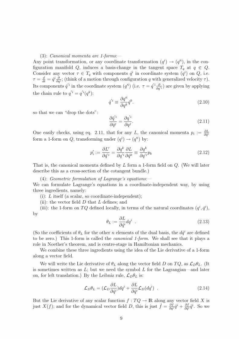
(3): Canonical momenta are 1-forms:—Any point transformation, or any coordinate transformation (qi) → (q′i), in the con-figuration manifold Q, induces a basis-change in the tangent space Tq at q ∈ Q.Consider any vector τ ∈ Tq with components qi in coordinate system (qi) on Q, i.e.τ = d

dt= qi ∂

∂qi ; (think of a motion through configuration q with generalized velocity τ).

Its components q′i in the coordinate system (q′i) (i.e. τ = q

′i ∂∂q′i ) are given by applying

the chain rule to q′i = q

′i(qk):

q′i ≡ ∂q′i

∂qkqk. (2.10)

so that we can “drop the dots”:∂q

′i

∂qj=

∂q′i

∂qj. (2.11)

One easily checks, using eq. 2.11, that for any L, the canonical momenta pi := ∂L∂qi

form a 1-form on Q, transforming under (qi) → (q′i) by:

p′i :=∂L′

∂q′i=

∂qk

∂q′i∂L

∂qk≡ ∂qk

∂q′ipk (2.12)

That is, the canonical momenta defined by L form a 1-form field on Q. (We will laterdescribe this as a cross-section of the cotangent bundle.)

(4): Geometric formulation of Lagrange’s equations:—We can formulate Lagrange’s equations in a coordinate-independent way, by usingthree ingredients, namely:

(i): L itself (a scalar, so coordinate-independent);(ii): the vector field D that L defines; and(iii): the 1-form on TQ defined locally, in terms of the natural coordinates (qi, qi),

by

θL :=∂L

∂qidqi . (2.13)

(So the coefficients of θL for the other n elements of the dual basis, the dqi are definedto be zero.) This 1-form is called the canonical 1-form. We shall see that it plays arole in Noether’s theorem, and is centre-stage in Hamiltonian mechanics.

We combine these three ingredients using the idea of the Lie derivative of a 1-formalong a vector field.

We will write the Lie derivative of θL along the vector field D on TQ, as LDθL. (Itis sometimes written as L; but we need the symbol L for the Lagrangian—and lateron, for left translation.) By the Leibniz rule, LDθL is:

LDθL = (LD∂L

∂qi)dqi +

∂L

∂qiLD(dqi) . (2.14)

But the Lie derivative of any scalar function f : TQ → IR along any vector field X isjust X(f); and for the dynamical vector field D, this is just f = ∂f

∂qi qi + ∂f

∂qi qi. So we

9

have

LDθL = (d

dt

∂L

∂qi)dqi +

∂L

∂qidqi . (2.15)

Rewriting the first term by the Lagrange equations, we get

LDθL = (∂L

∂qi)dqi +

∂L

∂qidqi ≡ dL . (2.16)

We can conversely deduce the familiar Lagrange equations from eq. 2.16, by takingcoordinates. So we conclude that these equations’ coordinate-independent form is:

LDθL = dL . (2.17)

(5): Towards the Hamiltonian framework:—Finally, a comment about the Lagrangian framework’s limitations as regards solvingproblems, and how they prompt the transition to Hamiltonian mechanics.

Recall the remark at the end of Section 2.1, that the n equations eq. 2.2 are ingeneral hard to solve for the qi(t0): they lie buried in the left hand side of eq. 2.2. On

the other hand, the n equations qi = dqi

dt(the second group of n equations in (1) above)

are as simple as can be.This makes it natural to seek another 2n-dimensional space of variables, ξα say

(α = 1, ..., 2n), in which:(i): a motion is described by first-order equations, so that we have the same

advantage as in TQ that a unique trajectory passes through each point of the space;but in which

(ii): all 2n equations have the simple form dξα

dt= fα(ξ1, ...ξ2n) for some set of

functions fα(α = 1, ..., 2n).Indeed, Hamiltonian mechanics provides exactly such a space: it is usually

the cotangent bundle of the configuration manifold, instead of its tangent bundle.But before turning to that, we expound Noether’s theorem in the current Lagrangianframework.

3 Noether’s theorem in Lagrangian mechanics

3.1 Preamble: a modest plan

Any discussion of symmetry in Lagrangian mechanics must include a treatment of“Noether’s theorem”. The scare quotes are to indicate that there is more than oneNoether’s theorem. Quite apart from Noether’s work in other branches of mathematics,her paper (1918) on symmetries and conserved quantities in Lagrangian theories hasseveral theorems. I will be concerned only with applying her first theorem to finite-dimensional systems. In short: it provides, for any continuous symmetry of a system’sLagrangian, a conserved quantity called the ‘momentum conjugate to the symmetry’.

10

I stress at the outset that the great majority of subsequent applications and com-mentaries (also for her other theorems, besides her first) are concerned with versionsof the theorems for infinite (i.e. continuous) systems. In fact, the context of Noether’sinvestigation was contemporary debate about how to understand conservation prin-ciples and symmetries in the “ultimate classical continuous system”, viz. gravitatingmatter as described by Einstein’s general relativity. This theory can be given a La-grangian formulation: that is, the equations of motion, i.e. Einstein’s field equations,can be deduced from a Hamilton’s Principle with an appropriate Lagrangian. Thecontemporary debate was especially about the conservation of energy and the principleof general covariance (also known as: diffeomorphism invariance). General covarianceprompts one to consider how a variational principle transforms under spacetime coor-dinate transformations that are arbitrary, in the sense of varying from point to point.This leads to the idea of “local” symmetries, which since Noether’s time has been im-mensely fruitful in both classical and quantum physics, and in both a Lagrangian andHamiltonian framework.7

So I agree that from the perspective of Noether’s work, and its enormous later de-velopment, this Section’s application of the first theorem to finite-dimensional systemsis, as they say, “trivial”. Furthermore, this application is easily understood, withouthaving to adopt that perspective, or even having to consider infinite systems. In otherwords: its statement and proof are natural, and simple, enough that the nineteenthcentury masters of mechanics, like Hamilton, Jacobi and Poincare, would certainlyrecognize it in their own work—allowing of course for adjustments to modern lan-guage. In fact, versions of it for the Galilei group of Newtonian mechanics and theLorentz group of special relativity were published a few years before Noether’s paper;(Brading and Brown (2003, p. 90); for details, cf. Kastrup (1987)).8

Nevertheless, it is worth expounding the finite-system version of Noether’s firsttheorem. For:

(i): It generalizes Section 2.1’s result about cyclic coordinates, and thereby theelementary theorems of the conservation of momentum, angular momentum and energywhich that result encompasses. The main generalization is that the theorem does notassume we have identified a cyclic coordinate. But on the other hand: every symmetryin the Noether sense will arise from a cyclic coordinate in some system q of generalizedcoordinates. (As we will see, this follows from the local existence and uniqueness ofsolutions of ordinary differential equations.)

(ii): This exposition will also prepare the way for our discussion of symmetry and

7Cf. Brading and Castellani (2003). Apart from papers specifically about Noether’s theorem, thisanthology’s papers by Wallace, Belot and Earman (all 2003) are closest to this paper’s concerns.

8Here again, ‘versions of it’ needs scare-quotes. For in what follows, I shall be more limited thanthese proofs, in two ways. (1): I limit myself, as I did in Section 2.2.1, both to time-independentLagrangians and to time-independent transformations: so my discussion does not encompass boosts.(2): I will take a symmetry of L to require that L be the very same; whereas some treatmentsallow the addition to L of the time-derivative of a function G(q) of the coordinates q—since such atime-derivative makes no difference to the Lagrange equations.

11

conserved quantities in Hamiltonian mechanics.9

In this exposition, I will also discuss en passant the distinction between:(i) the notion of symmetry at work in Noether’s theorem, i.e. a symmetry of L,

often called a variational symmetry; and(ii) the notion of a symmetry of the set of solutions of a differential equation: often

called a dynamical symmetry. This notion applies to all sorts of differential equations,and systems of them; not just to those with the form of Lagrange’s equations (i.e.derivable from an variational principle). In short, this sort of symmetry is a mapthat sends any solution of the given equation(s) (in effect: a dynamically possiblehistory of the system—a curve in the state-space) to some other solution. Finding suchsymmetries, and groups of them, is a central part of the modern theory of integrationof differential equations (both ordinary and partial).

Broadly speaking, this notion is more general than that of a symmetry of L. Notonly does it apply to many other sorts of differential equation. Also, for Lagrange’sequations: a symmetry of L is (with one caveat) a symmetry of the solutions, i.e. adynamical symmetry—but the converse is false.10

In this Section, the plan is as follows. We define:(i): a (continuous) symmetry as a vector field (on the configuration manifold Q)

that generates a family of transformations under which the Lagrangian is invariant;(Section 3.2);

(ii): the momentum conjugate to a vector field, as (roughly) the rate of change ofthe Lagrangian with respect to the qs in the direction of the vector field; (Section 3.3).

These two definitions lead directly to Noether’s theorem (Section 3.4): after all thestage-setting, the proof will be a one-liner application of Lagrange’s equations.

3.2 Vector fields and symmetries—variational and dynamical

I need to expound three topics:(1): the idea of a vector field on the configuration manifold Q; and how to lift it to

TQ;(2): the definition of a variational symmetry;(3): the contrast between (2) and the idea of dynamical symmetry.

Note that, as in previous Sections, I will often speak, for simplicity, “globally, notlocally”, i.e. as if the relevant scalar functions, vector fields etc. are defined on all of

9Other expositions of Noether’s theorem for finite-dimensional Lagrangian mechanics include:Arnold (1989: 88-89), Desloge (1982: 581-586), Lanczos (1986: 401-405: emphasizing the variationalperspective) and Johns (2005: Chapter 13). Butterfield (2004a, Section 4.7) is a more detailed versionof this Section. Beware: though many textbooks of Hamiltonian mechanics cover the Hamiltonianversion of Noether’s theorem (which, as we will see, is stronger), they often do not label it as such;and if they do label it, they often do not relate it clearly to the Lagrangian version.

10An excellent account of this modern integration theory, covering both ordinary and partial differ-ential equations, is given by Olver (2000). He also covers the Lagrangian case (Chapter 5 onwards),and gives many historical details especially about Lie’s pioneering contributions.

12

Q or TQ. Of course, they need not be.

3.2.1 Vector fields on TQ; lifting fields from Q to TQ

We recall first that a differentiable vector field on Q is represented in a coordinatesystem q = (q1, . . . , qn) by n first-order ordinary differential equations

dqi

dε= f i(q1, . . . , qn) . (3.1)

A vector field generates a one-parameter family of active transformations: viz. passagealong the vector field’s integral curves, by a varying parameter-difference ε. The vectorfield is called the infinitesimal generator of the family. It is common to write theparameter as τ , but in this Section we use ε to avoid confusion with t, which oftenrepresents the time.

Similarly, a vector field defined on TQ corresponds to a system of 2n ordinarydifferential equations, and generates an active transformation of TQ. But I will consideronly vector fields on TQ that mesh with the structure of TQ as a tangent bundle, inthe sense that they are induced by vector fields on Q, in the following natural way.

This induction has two ingredient ideas.First, any curve in Q (representing a possible state of motion) defines a correspond-

ing curve in TQ, because the functions qi(t) define the functions qi(t). (Here t is theparameter of the curve.) More formally: given any curve in configuration space, φ : I ⊂IR → Q, with coordinate expression in the q-system t ∈ I 7→ q(φ(t)) ≡ q(t) = qi(t), wedefine its extension to TQ to be the curve Φ : I ⊂ IR → TQ given in the correspondingcoordinates by qi(t), qi(t).

Second, any vector field X on Q generates displacements in any possible state ofmotion, represented by a curve in Q with coordinate expression qi = qi(t). Namely:for a given value of the parameter ε, the displaced state of motion is represented bythe curve in Q

qi(t) + εX i(qi(t)) . (3.2)

Putting these ingredients together: we first displace a curve within Q, and thenextend the result to TQ. Namely, the extension to TQ of the (curve representing)the displaced state of motion is given by the 2n functions, in two groups each of nfunctions, for the (q, q) coordinate system

qi(t) + εX i(qi(t)) and qi(t) + εY i(qi(t), qi) ; (3.3)

where Y is defined to be the vector field on TQ that is the derivative along the originalstate of motion of X. That is:

Y i(q, q) :=dX i

dt= Σj

∂X i

∂qjqj. (3.4)

13

Thus displacements by a vector field within Q are lifted to TQ. The vector field X onQ lifts to TQ as (X, dX

dt); i.e. it lifts to the vector field that sends a point (qi, qi) ∈ TQ

to (qi + εX i, qi + εdXi

dt).11

3.2.2 The definition of variational symmetry

To define variational symmetry, I begin with the integral notion and then give thedifferential notion. The idea is that the Lagrangian L, a scalar L : TQ → IR, shouldbe invariant under all the elements of a one-parameter family of active transformationsθε : ε ∈ I ⊂ IR: at least in a neighbourhood of the identity map corresponding to ε = 0,θ0 ≡ idU . (Here U is some open subset of TQ, maybe not all of it.)

That is, we define the family θε : ε ∈ I ⊂ IR to be a variational symmetry of Lif L is invariant under the transformations: L = L θε, at least around ε = 0. (Wecould use the correspondence between active and passive transformations to recast thisdefinition, and what follows, in terms of a passive notion of symmetry as sameness ofL’s functional form in different coordinate systems. I leave this as an exercise! Or cf.Butterfield (2004a: Section 4.7.2).)

For the differential notion of variational symmetry, we of course use the idea of avector field. But we also impose Section 3.2.1’s restriction to vector fields on TQ thatare induced by vector fields on Q. So we define a vector field X on Q that generatesa family of active transformations θε on TQ to be a variational symmetry of L if thefirst derivative of L with respect to ε is zero, at least around ε = 0. More precisely:writing

L θε = L(qi + εX i, qi + εY i) with Y i = Σj∂X i

∂qjqj , (3.5)

we say X is a variational symmetry iff the first derivative of L with respect to ε is zero(at least around ε = 0). That is: X is a variational symmetry iff

Σi X i ∂L

∂qi+ Σi Y i ∂L

∂qi= 0 with Y i = Σj

∂X i

∂qjqj . (3.6)

3.2.3 A contrast with dynamical symmetries

The general notion of a dynamical symmetry, i.e. a symmetry of some equations ofmotion (whether Euler-Lagrange or not), is not needed for Section 3.4’s presentationof Noether’s theorem. But the notion is so important that I must mention it, thoughonly to contrast it with variational symmetries.

The general definition is roughly as follows. Given any system of differential equa-tions, E say, a dynamical symmetry of the system is an active transformation ζ on the

11I have discussed this in terms of some system (q, q) of coordinates. But the definitions of extensionsand displacements are in fact coordinate-independent. Besides, one can show that the operations ofdisplacing a curve within Q, and extending it to TQ, commute to first order in ε: the result is thesame for either order of the operations.

14

system E ’s space of both independent variables, xj say, and dependent variables yi

say, such that any solution of E , yi = f i(xj) say, is carried to another solution. Fora precise definition, cf. Olver (2000: Def. 2.23, p. 93), and his ensuing discussion ofthe induced action (called ‘prolongation’) of the transformation ζ on the spaces of (ingeneral, partial) derivatives of the y’s with respect to the xs (i.e. jet spaces).

As I said in Section 3.1, groups of symmetries in this sense play a central role in themodern theory of differential equations: not just in finding new solutions, once given asolution, but also in integrating the equations. For some main theorems stating criteria(in terms of prolongations) for groups of symmetries, cf. Olver (2000: Theorem 2.27,p. 100, Theorem 2.36, p. 110, Theorem 2.71, p. 161).

But for present purposes, it is enough to state the rough idea of a one-parametergroup of dynamical symmetries (without details about prolongations!) for Lagrange’sequations in the familiar form, eq. 2.1.

In this simple case, there is just one independent variable x := t, so that:(a): we are considering ordinary, not partial, differential equations, with n depen-

dent variables yi := qi(t).(b): prolongations correspond to lifts of maps on Q to maps on TQ; cf. Section

3.2.1.Furthermore, in line with the discussion following Lagrange’s equations eq. 2.1, the

time-independence of the Lagrangian (time being a cyclic coordinate) means we candefine dynamical symmetries ζ in terms of active transformations on the tangent bun-dle, θ : TQ → TQ, that are lifted from active transformations on Q. In effect, we definesuch a map ζ by just adjoining to any such θ : TQ → TQ the identity map on the timevariable id : t ∈ IR 7→ t. (More formally: ζ : (q, q, t) ∈ TQ×IR 7→ (θ(q, q), t) ∈ TQ×IR.)

Then we define in the usual way what it is for a one-parameter family of such mapsζs : s ∈ I ⊂ IR to be a (local) one-parameter group of dynamical symmetries (forLagrange’s equations eq. 2.1): namely, if any solution curve q(t) (equivalently: itsextension q(t), q(t) to TQ) of the Lagrange equations is carried by each ζs to anothersolution curve, with the ζs for different s composing in the obvious way, for s closeenough to 0 ∈ I.

And finally: we also define (in a manner corresponding to the discussion at theend of Section 3.2.2) a differential, as against integral, notion of dynamical symme-try. Namely, we say a vector field X on Q is a dynamical symmetry if its lift to TQ(more precisely: its lift, with the identity map on the time variable adjoined) is theinfinitesimal generator of such a one-parameter family ζs.

For us, the important point is that this notion of a dynamical symmetry is differentfrom Section 3.2.2’s notion of a variational symmetry.12 As I announced in Section 3.1,a variational symmetry is (with one caveat) a dynamical symmetry—but the converseis false. Fortunately, the same simple example will serve both to show the subtlety

12Since the Lagrangian L is especially associated with variational principles, while the dynamics isgiven by equations of motion, calling Section 3.2.2’s notion ‘variational symmetry’, and this notion‘dynamical symmetry’ is a good and widespread usage. But beware: it is not universal.

15

about the first implication, and as a counterexample to the converse implication. Thisexample is the two-dimensional harmonic oscillator.13

The usual Lagrangian is, with cartesian coordinates written as qs, and the con-travariant indices written for clarity as subscripts:

L1 =1

2

[q21 + q2

2 − ω2(q21 + q2

2)]

; (3.7)

giving as Lagrange equations:

qi + ω2qi = 0 , i = 1, 2. (3.8)

But these Lagrange equations, i.e. the same dynamics, are also given by

L2 = q1q2 − ω2q1q2 . (3.9)

The rotations in the plane are of course a variational symmetry of L1, and a dynamicalsymmetry of eq. 3.8. But they are not a variational symmetry of L2. So a dynamicalsymmetry need not be a variational one. Besides, these equations contain anotherexample to the same effect. Namely, the “squeeze” transformations

q′1 := eηq1 , q′2 := e−ηq2 (3.10)

are a dynamical symmetry of eq. 3.8, but not a variational symmetry of L1. So again:a dynamical symmetry need not be a variational one.14

I turn to the first implication: that every variational symmetry is a dynamicalsymmetry. This is true: general and abstract proofs (applying also to continuoussystems i.e. field theories) can be found in Olver (2000: theorem 4.14, p. 255; theorem4.34, p. 278; theorem 5.53, p. 332).

But beware of a condition of the theorem. (This is the caveat mentioned at the endof Section 3.1.) The theorem requires that all the variables q (for continuous systems:all the fields φ) be subject to Hamilton’s Principle. The need for this condition is shownby rotations in the plane, which are a variational symmetry of the familiar LagrangianL1 above. But it is easy to show that such a rotation is a dynamical symmetry of oneof the Lagrange equations, say the equation for the variable q1

q1 + ω2q1 = 0 , (3.11)

only if the corresponding Lagrange equation holds for q2.

13All the material to the end of this Subsection is drawn from Brown and Holland (2004a); cf. alsotheir (2004). The present use of the harmonic oscillator example also occurs in Morandi et al (1990:203-204).

14In the light of this, you might ask about a more restricted implication: viz. must every dynamicalsymmetry of a set of equations of motion be a variational symmetry of some or other Lagrangianthat yields the given equations as the Euler-Lagrange equations of Hamilton’s Principle? Again, theanswer is No for the simple reason that there are many (sets of) equations of motion that are notEuler-Lagrange equations of any Lagrangian, and yet have dynamical symmetries.

Wigner (1954) gives an example. The general question of under what conditions is a set of ordinarydifferential equations the Euler-Lagrange equations of some Hamilton’s Principle is the inverse problemof Lagrangian mechanics. It is a large subject with a long history; cf. e.g. Santilli (1979), Lopuszanski(1999).

16

3.3 The conjugate momentum of a vector field

Now we define the momentum conjugate to a vector field X to be the scalar functionon TQ:

pX : TQ → IR ; pX = Σi X i ∂L

∂qi(3.12)

(For a time-dependent Lagrangian, pX would be a scalar function on TQ× IR, with IRrepresenting time.)

We shall see in the next Subsection’s examples that this definition generalizes in anappropriate way Section 2.1’s definition of the momentum conjugate to a coordinate q.

But first note that it is an improvement in the sense that, while the momentumconjugate to a coordinate q depends on the choice made for the other coordinates, themomentum pX conjugate to a vector field X is independent of the coordinates chosen.Though this point is not needed in order to prove Noether’s theorem, here is the proof.

We first apply the chain-rule to L = L(q′(q), q′(q, q)) and eq. 2.11 (“cancellation ofthe dots”), to get

∂L

∂qi= Σj

∂L

∂q′j∂q′j

∂qi= Σj

∂L

∂q′j∂q′j

∂qi. (3.13)

Then using the transformation law for components of a vector field

X ′i = Σj∂q′i

∂qjXj. (3.14)

and relabelling i and j, we deduce:

p′X = Σi X ′i ∂L

∂q′i= Σij Xj ∂q′i

∂qj

∂L

∂q′i= Σij X i ∂q′j

∂qi

∂L

∂q′j= Σi X i ∂L

∂qi≡ pX . (3.15)

Finally, I remark incidentally that in the geometric formulation of Lagrangian me-chanics (Section 2.2) , the coordinate-independence of pX becomes, unsurprisingly, atriviality. Namely: pX is obviously the contraction of X as lifted to TQ with thecanonical 1-form on TQ that we defined in eq. 2.13:

θL :=∂L

∂qidqi . (3.16)

We will return to this at the end of Section 3.4.1.

3.4 Noether’s theorem; and examples

Given just the definition of conjugate momentum, eq. 3.12, the proof of Noether’stheorem is immediate. (The interpretation and properties of this momentum, discussedin the last Subsection, are not needed.) The theorem says:

17

Noether’s theorem for Lagrangian mechanics If X is a (variational)symmetry of a system with Lagrangian L(q, q, t), then X’s conjugate mo-mentum is a constant of the motion.

Proof: We just calculate the derivative of the momentum eq. 3.12 along the solu-tion curves in TQ, and apply Lagrange’s equations and the definitions of Y i, and ofsymmetry eq. 3.6:

dp

dt= Σi

dX i

dt

∂L

∂qi+ Σi X i d

dt

(∂L

∂qi

)(3.17)

= Σi Y i ∂L

∂qi+ Σi X i ∂L

∂qi= 0 . QED.

Examples:— This proof, though neat, is a bit abstract! So here are two examples,both of which return us to examples we have already seen.

(1): The first example is a shift in a cyclic coordinate qn: i.e. the case with whichour discussion of Noether’s theorem began at the end of Section 2.1. So suppose qn iscyclic, and define a vector field X by

X1 = 0, . . . , Xn−1 = 0, Xn = 1 . (3.18)

So the displacements generated by X are translations by an amount ε in the qn-direction. Then Y i := dXi

dtvanishes, and the definition of (variational) symmetry

eq. 3.6 reduces to∂L

∂qn= 0 . (3.19)

So since qn is assumed to be cyclic, X is a symmetry. And the momentum conjugateto X, which Noether’s theorem tells us is a constant of the motion, is the familiar one:

pX := Σi X i ∂L

∂qi=

∂L

∂qn. (3.20)

As mentioned in Section 3.1, this example is universal, in that every symmetry Xarises, around any point where X is non-zero, from a cyclic coordinate in some localsystem of coordinates. This follows from the basic theorem about the local existenceand uniqueness of solutions of ordinary differential equations. We can state the theoremas follows; (cf. e.g. Arnold (1973: 48-49, 77-78, 249-250), Olver (2000: Prop 1.29)).

Consider a system of n first-order ordinary differential equations on an open subsetU of an n-dimensional manifold

qi = X i(q) ≡ X i(q1, ..., qn) , q ∈ U ; (3.21)

equivalently, a vector field X on U . Let q0 be a non-singular point of the vector field,i.e. X(q0) 6= 0. Then in a sufficiently small neighbourhood V of q0, there is a coordinate

18

system (formally, a diffeomorphism f : V → W ⊂ IRn) such that, writing yi : IRn → IRfor the standard coordinates on W and ei for the ith standard basic vector of IRn, eq.3.21 goes into the very simple form

y = en; i.e. yn = 1, y1 = y2 = . . . = yn−1 = 0 in W . (3.22)

(In terms of the tangent map (also known as: push-forward) f∗ on tangent vectors thatis induced by f : f∗(X) = en in W .) On account of eq. 3.22’s simple form, Arnoldsuggests the theorem might well be called the ‘rectification theorem’.

We should note two points about the theorem:(i): The rectifying coordinate system f may of course be very hard to find. So the

theorem by no means makes all problems “trivially soluble”; cf. again footnote 4.(ii): The theorem has an immediate corollary about local constants of the motion.

Namely: n first-order ordinary differential equations have, locally, n − 1 functionallyindependent constants of the motion (also known as: first integrals). They are given,in the above notation, by y1, . . . , yn−1.

We now apply the rectification theorem, so as to reverse the reasoning in the aboveexample of qn cyclic. That is: assuming X is a symmetry, let us rectify it—i.e. let uspass to a coordinate system (q) such that eq. 3.18 holds. Then, as above, Y i := dXi

dt

vanishes; and X’s being a (variational) symmetry, eq. 3.6, reduces to qn being cyclic;and the momentum conjugate to X, pX reduces to the familiar conjugate momentumpn = ∂L

∂qn . Thus every symmetry X arises locally from a cyclic coordinate qn and the

corresponding conserved momentum is pn. (But note that this may hold only “verylocally”: the domain V of the coordinate system f in which X generates displacementsin the direction of the cyclic coordinate qn can be smaller than the set U on which Xis a symmetry.)

In Section 5.3, the fact that every symmetry arises locally from a cyclic coordinatewill be important for understanding the Hamiltonian version of Noether’s theorem.

(2): Let us now look at our previous example, the angular momentum of a freeparticle (eq. 2.6), in the cartesian coordinate system, i.e. a coordinate system withoutcyclic coordinates. So let q1 := x, q2 := y, q3 := z. (In this example, subscripts willagain be a bit clearer.) Then a small rotation about the x-axis

δx = 0, δy = −εz, δz = εy (3.23)

corresponds to a vector field X with components

X1 = 0, X2 = −q3, X3 = q2 (3.24)

so that the Yi areY1 = 0, Y2 = −q3, X3 = q2 . (3.25)

For the Lagrangian

L =1

2m(q2

1 + q22 + q2

3) (3.26)

19

X is a (variational) symmetry since the definition of symmetry eq. 3.6 now reduces to

Σi Xi∂L

∂qi

+ Σi Yi∂L

∂qi

= −q3∂L

∂q2

+ q2∂L

∂q3

= 0 . (3.27)

So Noether’s theorem then tells us that X’s conjugate momentum is

pX := Σi Xi∂L

∂qi

= X2∂L

∂q2

+ X3∂L

∂q3

= −mzy + myz (3.28)

which is indeed the x-component of angular momentum.

3.4.1 A geometrical formulation

We can give a geometric formulation of Noether’s theorem by using the vanishing ofthe Lie derivative to express constancy along the integral curves of a vector field. Thereare two vector fields on TQ to consider: the dynamical vector field D (cf. eq. 2.8),and the lift to TQ of the vector field X that is the variational symmetry.

I will now write X for this lift. So given the vector field X on Q

X = X i(q)∂

∂qi, (3.29)

the lift X of X to TQ is, by eq. 3.4,

X = X i(q)∂

∂qi+

∂X i(q)

∂qjqj ∂

∂qi, (3.30)

where the q argument of X i emphasises that the X i do not depend on q.

That X is a variational symmetry means that in TQ, the Lie derivative of L alongthe lift X vanishes: LXL = 0. On the other hand, we know from eq. 3.16 that themomentum pX conjugate to X is the contraction <; > of X with the canonical 1-formθL := ∂L

∂qi dqi on TQ:

pX := X i ∂L

∂qi≡ < X; θL > . (3.31)

So Noether’s theorem says:

If LXL = 0, then LD < X; θL >= 0.

Note finally that eq. 3.31 shows that the theorem has no converse. That is: giventhat a dynamical variable p : TQ → IR is a constant of the motion, LDp = 0, thereis no single vector field X on TQ such that p =< X; θL >. For given such a X, onecould get another by adding any field Y for which < Y ; θL >= 0. However, we will seein Section 5.2 that in Hamiltonian mechanics a constant of the motion does determinea corresponding vector field on the state space.

20

4 Hamiltonian mechanics introduced

4.1 Preamble

From now on this paper adopts the Hamiltonian framework. As we shall see, its de-scription of symmetry and conserved quantities is in various ways more straightforwardand powerful than that of the Lagrangian framework.

The main idea is to replace the qs by the canonical momenta, the ps. More gener-ally, the state-space is no longer the tangent bundle TQ but a phase space Γ, which wetake to be the cotangent bundle T ∗Q. (Here, the phrase ‘we take to be’ just signals thefact that eventually, in Section 6.8, we will glimpse a more general kind of Hamiltonianstate-space, viz. Poisson manifolds.)

Admittedly, the theory on TQ given by Lagrange’s equations eq. 2.1 is equivalentto the Hamiltonian theory on T ∗Q given by eq. 4.5 below, once we assume the Hessiancondition eq. 2.3.

But of course, theories can be formally equivalent, but different as regards theirpower for solving problems, their heuristic value and even their interpretation. In ourcase, two advantages of Hamiltonian mechanics over Lagrangian mechanics are com-monly emphasised. (i): The first concerns its greater power or flexibility for describinga given system, that Lagrangian methods can also describe (and so its greater powerfor solving problems about such a system). (ii): The second concerns the broader ideaof describing other systems. In more detail:—

(i): Hamiltonian mechanics replaces the group of point transformations, q → q′ onQ, together with their lifts to TQ, by a “corresponding larger” group of transforma-tions on Γ, the group of canonical transformations (also known as, for the standardcase where Γ = T ∗Q: the symplectic group).

This group “corresponds” to the point transformations (and their lifts) in thatwhile for any Lagrangian L, Lagrange’s equations eq. 2.1 are covariant under all thepoint transformations, Hamilton’s equations eq. 4.5 below are (for any HamiltonianH) covariant under all canonical transformations. And it is a “larger” group because:

(a) any point transformation together with its lift to TQ is a canonical transforma-tion: (more precisely: it naturally defines a canonical transformation on T ∗Q);

(b) not every canonical transformation is thus induced by a point transformation;for a canonical transformation can “mix” the qs and ps in a way that point transfor-mations and their lifts cannot.

There is a rich and multi-faceted theory of canonical transformations, to whichthere are three main approaches—generating functions, integral invariants and sym-plectic geometry. I will adopt the symplectic approach, but not need many detailsabout it. In particular, we will need only a few details about how the “larger” groupof canonical transformations makes for a more powerful version of Noether’s theorem.

(ii): The Hamiltonian framework connects analytical mechanics with other fieldsof physics, especially statistical mechanics and optics. The first connection goes via

21

canonical transformations, especially using the integral invariants approach. The sec-ond connection goes via Hamilton-Jacobi theory; (for a philosopher’s exposition, withan eye on quantum theory, cf. Butterfield (2004b: especially Sections 7-9)).15

With its theme of symmetry and conservation, this paper will illustrate (i), greaterpower in describing a given system, rather than (ii), describing other systems. As to(i), we will see two main ways in which the Hamiltonian framework is more powerfulthan the Lagrangian one. First, cyclic coordinates will “do more work for us” (Section4.2). Second, the Hamiltonian version of Noether’s theorem is both: more powerful,thanks to the use of the “larger” group of canonical transformations; and more easilyproven, thanks to the use of Poisson brackets (Section 5).

So from now on, the broad plan is as follows. After Section 4.2’s deduction of Hamil-ton’s equations, Section 4.3 introduces symplectic structure, starting from the “naive”form of the symplectic matrix. Section 5 presents Poisson brackets, and the Hamil-tonian version of Noether’s theorem. Finally, Section 6 gives a geometric perspective,corresponding to Section 2.2’s geometric perspective on the Lagrangian framework.

4.2 Hamilton’s equations

4.2.1 The equations introduced

Recall the vision in (5) of Section 2.2.2: that we seek 2n new variables, ξα say, α =1, ..., 2n in which Lagrange’s equations take the simple form

dξα

dt= fα(ξ1, ...ξ2n) . (4.1)

We can find the desired variables ξα by using the canonical momenta

pi :=∂L

∂qi=: Lqi , (4.2)

to write the 2n Lagrange equations as

dpi

dt=

∂L

dqi;

dqi

dt= qi . (4.3)

These are of the desired simple form, except that the right hand sides need to be writtenas functions of (q, p, t) rather than (q, q, t). (Here and in the next two paragraphs, wetemporarily allow time-dependence, since the deduction is unaffected: the time variableis “carried along unaffected”. In the terms of Section 2.1, this means allowing non-scleronomous constraints and a time-dependent work-function U .)

15Of course, some aspects of Hamiltonian mechanics illustrate both (i) and (ii). For example,Liouville’s theorem on the preservation of phase space volume illustrates both (i)’s integral invariantsapproach to canonical transformations and (ii)’s connection to statistical mechanics.

22

For the second group of n equations, this is in principle straightforward, given ourassumption of a non-zero Hessian, eq. 2.3. This implies that we can invert eq. 4.2 soas to get the n qi as functions of (q, p, t). We can then apply this to the first group ofequations; i.e. we substitute qi(q, p, t) wherever qi appears in any right hand side ∂L

dqi .

But we need to be careful: the partial derivative of L(q, q, t) with respect to qi isnot the same as the partial derivative of L(q, p, t) := L(q, q(q, p, t), t) with respect toqi, since the first holds fixed the qs, while the second holds fixed the ps. A comparisonof these partial derivatives leads, with algebra, to the result that if we define theHamiltonian function by

H(q, p, t) := piqi(q, p, t)− L(q, p, t) (4.4)

then the 2n equations eq. 4.3 go over to Hamilton’s equations

dpi

dt= −∂H

∂qi;

dqi

dt=

∂H

∂pi

. (4.5)

So we have cast our 2n equations in the simple form, dξα

dt= fα(ξ1, ...ξ2n), requested in

(5) of Section 2.2. More explicitly: defining

ξα = qα, α = 1, ..., n ; ξα = pα−n, α = n + 1, ..., 2n (4.6)

Hamilton’s equations become

ξα =∂H

∂ξα+n, α = 1, ..., n ; ξα = − ∂H

∂ξα−n, α = n + 1, ..., 2n . (4.7)

To sum up: a single function H determines, through its partial derivatives, the evolu-tion of all the qs and ps—and so, the evolution of the state of the system.

4.2.2 Cyclic coordinates in the Hamiltonian framework

Just from the form of Hamilton’s equations, we can immediately see a result thatis significant for our theme of how symmetries and conserved quantities reduce thenumber of variables involved in a problem. In short, we can see that with Hamilton’sequations in hand, cyclic coordinates will “do more work for us” than they do in theLagrangian framework.

More specifically, recall the basic Lagrangian result from the end of Section 2.1, thatthe generalized momentum pn := ∂L

∂qn is conserved if, indeed iff, its conjugate coordinate

qn is cyclic, ∂L∂qn = 0. And recall from Section 3.4 that this result underpinned Noether’s

theorem in the precise sense of being “universal” for it. Corresponding results hold inthe Hamiltonian framework—but are in certain ways more powerful.

Thus we first observe that the transformation “from the qs to the ps”, i.e. thetransition between Lagrangian and Hamiltonian frameworks, does not involve the de-pendence on the qs. More precisely: partially differentiating eq. 4.4 with respect to

23

qn, we obtain∂H

∂qn≡ ∂H

∂qn|p;qi,i6=n = − ∂L

∂qn≡ ∂L

∂qn|q;qi,i 6=n . (4.8)

(The other two terms are plus and minus pi∂qi

∂qn , and so cancel.) So a coordinate qn

that is cyclic in the Lagrangian sense is also cyclic in the obvious Hamiltonian sense,viz. that ∂H

∂qn = 0. But by Hamilton’s equations, this is equivalent to pn = 0. So we

have the result corresponding to the Lagrangian one: pn is conserved iff qn is cyclic (inthe Hamiltonian sense).

We will see in Section 5.3 that this result underpins the Hamiltonian version ofNoether’s theorem; just as the corresponding Lagrangian result underpinned the La-grangian version of Noether’s theorem (cf. discussion after eq. 3.20).

But we can already see that this result gives the Hamiltonian formalism an advan-tage over the Lagrangian. In the latter, the generalized velocity corresponding to acyclic coordinate, qn will in general still occur in the Lagrangian. The Lagrangian willbe L(q1, . . . , qn−1, q1, . . . , qn, t), so that we still face a problem in n variables.

But in the Hamiltonian formalism, pn will be a constant of the motion, α say, sothat the Hamiltonian will be H(q1, . . . , qn−1, p1, . . . , pn−1, α, t). So we now face a prob-lem in n − 1 variables, α being simply determined by the initial conditions. That is:after solving the problem in n − 1 variables, qn is determined just by quadrature: i.e.just by integrating (perhaps numerically) the equation

qn =∂H

∂α, (4.9)

where, thanks to having solved the problem in n − 1 variables, the right-hand side isnow an explicit function of t.

This result is very simple. But it is an important illustration of the power of theHamiltonian framework. Indeed, Arnold remarks (1989: 68) that ‘almost all the solvedproblems in mechanics have been solved by means of’ it!

No doubt his point is, at least in part, that this result underpins the Hamiltonianversion of Noether’s theorem. But I should add that the result also motivates thestudy of various notions related to the idea of cyclic coordinates, such as constants ofthe motion being in involution (i.e. having zero Poisson bracket with each other), anda system being completely integrable (in the sense of Liouville). These notions haveplayed a large part in the way that Hamiltonian mechanics has developed, especiallyin its theory of canonical transformations. And they play a large part in the wayHamiltonian mechanics has solved countless problems. But as announced in Section4.1, this paper will not go into these aspects of Hamiltonian mechanics, since they arenot needed for our theme of symmetry and conservation; (for a philosophical discussionof these aspects, cf. Butterfield 2005).

24

4.2.3 The Legendre transformation and variational principles

To end this Subsection, I note two aspects of this transition from Lagrange’s equationsto Hamilton’s. For, although I shall not need details about them, they each lead to arich theory:

(i): The transformation “from the qs to the ps” is the Legendre transformation. Ithas a striking geometric interpretation. In the simplest case, it concerns the fact thatone can describe a smooth convex real function y = f(x), f ′′(x) > 0, not by the pairsof its arguments and values (x, y), but by the pairs of its gradients at points (x, y)and the intercepts of its tangent lines with the y-axis. Given the non-zero Hessian (eq.2.3), one readily proves various results: e.g. that the geometric interpretation extendsto higher dimensions, and that the transformation is self-inverse, i.e. its square is theidentity. For details, cf. e.g.: Arnold (1989: Chapters 3.14, 9.45.C), Courant andHilbert (1953: Chapter IV.9.3; 1962, Chapter I.6), Jose and Saletan (1998: 212-217),Lanczos (1986: Chapter VI.1-4). The Legendre transformation is also described usingmodern geometry’s idea of a fibre derivative; as we will see briefly in Section 6.7.

(ii): The transition to Hamilton’s equations has achieved more than we initiallysought with our eq. 4.1. Namely: all the fα, all the right hand sides in Hamilton’sequations, are up to a sign, partial derivatives of a single function H. In the Hamil-tonian framework, it is precisely this feature that underpins the possibility of expressingthe equations of motion by variational principles; (of course, the Lagrangian frameworkhas a corresponding feature). But as I mentioned, this paper does not discuss vari-ational principles; for details cf. e.g. Lanczos (1986: Chapter VI.4) and Butterfield(2004: especially Section 5.2).

To sum up this introduction to Hamilton’s equations:— Even once we set aside(i) and (ii), these equations mark the beginning of a rich and multi-faceted theory.At the centre lies the 2n-dimensional phase space Γ coordinatized by the qs and ps:or more precisely, as we shall see later, the cotangent bundle T ∗Q. The structure ofHamiltonian mechanics is encoded in the structure of Γ, and thereby in the coordinatetransformations on Γ that preserve this structure, especially the form of Hamilton’sequations: the canonical transformations. As I mentioned in Section 4.1, these trans-formations can be studied from three main perspectives: generating functions, integralinvariants and symplectic structure—but I shall only need the last.

4.3 Symplectic forms on vector spaces

I shall introduce symplectic structure by giving Hamilton’s equations a yet more sym-metric appearance. This will lead to some elementary ideas about area in IRm andsymplectic forms on vector spaces: ideas which will later be “made local” by takingthe relevant copy of IRm to be the tangent space at a point of a manifold. (As usuallyformulated, Hamiltonian mechanics is especially concerned with the case m = 2n.)

25

4.3.1 Time-evolution from the gradient of H

Writing 1 and 0 for the n × n identity and zero matrices respectively, we define the2n× 2n symplectic matrix ω by

ω :=

(0 1−1 0

). (4.10)

ω is antisymmetric, and has the properties, writing ˜ for the transpose of a matrix,that

ω = −ω = ω−1 so that ω2 = −1 ; also det ω = 1. (4.11)

Using ω, Hamilton’s equations eq. 4.7 get the more symmetric form, in matrix notation

ξ = ω∂H

∂ξ. (4.12)

In terms of components, writing ωαβ for the matrix elements of ω, and defining ∂α :=∂ /∂ξα, eq. 4.7 become

ξα = ωαβ∂βH. (4.13)

Eq. 4.12 and 4.13 show how ω forms, from the naive gradient (column vector) ∇Hof H on the phase space Γ of qs and ps, the vector field on Γ that gives the system’sevolution: the Hamiltonian vector field, often written XH . At a point z = (q, p) ∈ Γ,eq. 4.12 can be written

XH(z) = ω∇H(z). (4.14)

The vector field XH is also written as D (for ‘dynamics’), on analogy with the La-grangian framework’s vector field D of eq. 2.8 in Section 2.2.

In Section 6, we will see how this definition of a vector field from a gradient, i.e. acovector or 1-form field, arises from Γ’s being a cotangent bundle. More precisely, wewill see that any cotangent bundle has an intrinsic symplectic structure that provides,at each point of the base-manifold, a natural i.e. basis-independent isomorphism be-tween the tangent space and the cotangent space. For the moment, we:

(i) note a geometric interpretation of ω in terms of area (Section 4.3.2); and then(ii) generalize the above discussion of ω into the definition of a symplectic form for

a fixed vector space (Section 4.3.3).

4.3.2 Interpretation in terms of areas

Let us begin with the simplest possible case: IR2 3 (q, p), representing the phase spaceof a particle constrained to one spatial dimension. Here, the 2× 2 matrix

ω :=

(0 1−1 0

)(4.15)

26

defines the antisymmetric bilinear form on IR2:

A : ((q1, p1), (q2, p2)) ∈ IR2 × IR2 7→ q1p2 − q2p1 ∈ IR (4.16)

since

q1p2 − q2p1 =(

q1 p1

) (0 1−1 0

)(q2

p2

)= det

(q1 q2

p1 p2

). (4.17)

It is easy to prove that A((q1, p1), (q2, p2)) ≡ q1p2 − q2p1 is the signed area of the

parallelogram spanned by (q1, p1), (q2, p2), where the sign is positive (negative) if the

shortest rotation from (q1, p1) to (q2, p2) is anti-clockwise (clockwise).

Similarly in IR2n: the matrix ω of eq. 4.10 defines an antisymmetric bilinear formon IR2n whose value on a pair (q, p) ≡ (q1, ...qn; p1, ..., pn), (q′, p′) ≡ (q′1, ...q′n; p′1, ..., p

′n)

is the sum of the signed areas of the n parallelograms formed by the projections of thevectors (q, p), (q′, p′) onto the n pairs of coordinate planes labelled 1, ..., n. That is tosay, the value is:

Σni=1 qip′i − q′ipi . (4.18)

This induction of bilinear forms from antisymmetric matrices can be generalized:there is a one-to-one correspondence between forms and matrices. In more detail:there is a one-to-one correspondence between antisymmetric bilinear forms on IR2 andantisymmetric 2×2 matrices. It is easy to check that any such form, ω say, is given, for

any basis v, w of IR2, by the matrix

(0 ω(v, w)

−ω(v, w) 0

). Similarly for any integer

n: one easily shows that there is a one-to-one correspondence between antisymmetricbilinear forms on IRn and antisymmetric n×n matrices. (In Hamiltonian mechanics asusually formulated, we consider the case where n is even and the matrix is non-singular,as in eq. 4.10. But when one generalizes to Poisson manifolds (cf. Section 6.8) oneallows n to be odd, and the matrix to be singular.)

This geometric interpretation of ω is important for two reasons.(i): The first reason is that the idea of an antisymmetric bilinear form on a copy of

IR2n is the main part of the definition of a symplectic form, which is the central notionin the usual geometric formulation of Hamiltonian mechanics. More details in Section4.3.3, for a fixed copy of IR2n; and in Section 6, where the form is defined on manycopies of IR2n, each copy being the tangent space at a point in the cotangent bundleT ∗Q.

(ii): The second reason is that the idea of (signed) area underpins the theory offorms (1-forms, 2-forms etc.): i.e. antisymmetric multilinear functions on products ofcopies of IRn. And when these copies of IRn are copies of the tangent space at (one andthe same) point in a manifold, these forms lead to the whole theory of integration onmanifolds. One needs this theory in order to make rigorous sense of any integration ona manifold beyond the most elementary (i.e. line-integrals); so it is crucial for almostany mathematical or physical theory using manifolds. In particular, it is crucial for

27

Hamiltonian mechanics. So no wonder the maestro says that ‘Hamiltonian mechanicscannot be understood without differential forms’ (Arnold 1989, p. 163).

However, it turns out that this paper will not need many details about forms and thetheory of integration. This is essentially because we focus only on solving mechanicalproblems, and simplifying them by appeals to symmetry. This means we will focuson line-integrals: viz. integrating with respect to time the equations of motion; orequivalently, integrating the dynamical vector field on the state space. We have alreadyseen this vector field as XH in eq. 4.14; and we will see it again, for example in termsof Poisson brackets (eq. 5.14), and in geometric terms (Section 6). But throughout,the main idea will be as suggested by eq. 4.14: the vector field is determined by thesymplectic matrix, “at” each point in the manifold Γ, acting on the gradient of theHamiltonian function H.

So in short: focussing on line-integrals enables us to side-step most of the theoryof forms.16

4.3.3 Bilinear forms and associated linear maps

We now generalize from the symplectic matrix ω to a symplectic form; in five extendedcomments.

(1): Preliminaries:—Let V be a (real finite-dimensional) vector space, with basis e1, ..., ei, ...en. We writeV ∗ for the dual space, and e1, ..., ei, ...en for the dual basis: ei(ej) := δi

j.

We recall that the isomorphism ei 7→ ei is basis-dependent: for a different basis,the corresponding isomorphism would be a different map. Only with the provision ofappropriate extra structure would this isomorphism be basis-independent.

For physicists, the most familiar example of such a structure is the spacetime metricg in relativity theory. In terms of components, this basis-independence shows up inthe way that g and its inverse lower and raise indices. As we will see in a moment, theunderlying mathematical point is that because g is a bilinear form on a vector spaceV , i.e. g : V × V → IR, and is non-degenerate, any v ∈ V defines, independently ofany choice of basis, an element of V ∗: viz. the map u ∈ V 7→ g(u, v). (In fact, V isthe tangent space at a spacetime point; but this physical interpretation is irrelevantto the mathematical argument.) We will also see that Hamiltonian mechanics hasa non-degenerate bilinear form, viz. a symplectic form, that similarly gives a basis-independent isomorphism between a vector space and its dual. (Roughly speaking, thisvector space will be the 2n-dimensional space of the qs and ps.)

On the other hand: for any vector space V , the isomorphism between V and V ∗∗

given byei 7→ [ei] ∈ V ∗∗ : ej ∈ V ∗ 7→ ej(ei) = δj

i (4.19)

16But forms are essential for understanding integration over surfaces of dimension two or more:which one needs for the integral invariants approach to Hamiltonian mechanics, and its deep connectionwith Stokes’ theorem.

28

is basis-independent, and so we identify ei with [ei], and V with V ∗∗. We will write< ; > (also written < , >) for the natural pairing (in either order) of V and V ∗: e.g.< ei ; ej > = < ej ; ei > = δj

i .

A linear map A : V → W induces (basis-independently) a transpose (aka: dual),written A (or AT or A∗), A : W ∗ → V ∗ by

∀α ∈ W ∗,∀v ∈ V : A(α)(v) ≡ < A(α) ; v > := α(A(v)) ≡ (α A)(v) . (4.20)

If A : V → W is a linear map between real finite-dimensional vector spaces, itsmatrix with respect to bases e1, ..., ei, ...en and f1, ..., fj, ...fm of V and W is given by:

A(ei) = Ajifj ; i.e. with v = viei, (A(v))j = Aj

ivi . (4.21)

So the upper index labels rows, and the lower index labels columns. Similarly, ifA : V ×W → IR is a bilinear form, its matrix for these bases is defined as

Aij := A(ei, fj) (4.22)

so that on vectors v = viei, w = wjfj, we have: A(v, w) = viAijwj.

(2): Associated maps and forms:—Given a bilinear form A : V×W → IR, we define the associated linear map A[ : V → W ∗

byA[(v)(w) := A(v, w) . (4.23)

Then A[(ei) = Aijfj: for both sides send any w = wjfj to Aijw

j. That is: the matrixof A[ in the bases ei, f

j of V and W ∗ is Aij:

[A[]ij = Aij. (4.24)

On the other hand, we can proceed from linear maps to associated bilinear forms.Given a linear map B : V → W ∗, we define the associated bilinear form B] on V ×W ∗∗ ∼= V ×W by

B](v, w) = < B(v) ; w > . (4.25)

If we put A[ for B in eq. 4.25, its associated bilinear form, acting on vectors v =viei, w = wjfj, yields, by eq. 4.23:

(A[)](v, w) = < A[(v) ; w > = A(v, w) . (4.26)

One similarly shows that if B : V → W ∗, then ∀w ∈ W :

(B])[(v)(w) ≡< (B])[(v) ; w > = B(v)(w) ≡< B(v) ; w > so that (B])[ = B .(4.27)

So the flat and sharp operations, [ and ], are inverses.

(3): Tensor products:—It will sometimes be helpful to put the above ideas in terms of tensor products. If

29

v ∈ V,w ∈ W , we can think of v and w as elements of V ∗∗,W ∗∗ respectively. Sowe define their tensor product as a bilinear form on V ∗ × W ∗ by requiring for allα ∈ V ∗, β ∈ W ∗:

(v ⊗ w)(α, β) := v(α)w(β) ≡ < v ; α >< w ; β > . (4.28)

Similarly for other choices of vector spaces or their duals. Given α ∈ V ∗, β ∈ W ∗, theirtensor product is a bilinear form on V ×W :

(α⊗ β)(v, w) := α(v)β(w) ≡ < v ; α >< w ; β > . (4.29)

Similarly, we can think of α ∈ V ∗, w ∈ W as elements of V ∗ and W ∗∗ respectively, andso define their tensor product as a bilinear form on V ×W ∗:

(α⊗ w)(v, β) := α(v)w(β) ≡ < v ; α >< w ; β > . (4.30)

In this way we can express the linear map A : V → W in terms of tensor products.Since

A(ei) = Ajifj iff < A(ei); f

j > = Aji (4.31)

eq. 4.30 implies thatA = Aj

i ei ⊗ fj . (4.32)

Similarly, a bilinear form A : V ×W → IR with matrix Aij := A(ei, fj) (cf. eq. 4.22)is:

A = Aij ei ⊗ f j (4.33)

The definitions of tensor product eq. 4.28, 4.29 and 4.30 generalize to higher-ranktensors (i.e. multilinear maps whose domains have more than two factors). But wewill not need these generalizations.

(4): Antisymmetric and non-degenerate forms:—We now specialize to the forms and maps of central interest in Hamiltonian mechanics.We take W = V , dim(V )=n, and define a bilinear form ω : V × V → IR to be:

(i): antisymmetric iff: ω(v, v′) = −ω(v, v′);(ii): non-degenerate iff: if ω(v, v′) = 0 ∀v′ ∈ V , then v = 0.

The form ω and its associated linear map ω[ : V → V ∗ now have a square matrix ωij

(cf. eq. 4.24). We define the rank of ω to be the rank of this matrix: equivalently, thedimension of the range ω[(V ).

We will also need the antisymmetrized version of eq. 4.29 that is definable whenW = V . Namely, we define the wedge-product of α, β ∈ V ∗ to be the antisymmetricbilinear form on V , given by

α ∧ β : (v, w) ∈ V × V 7→ (α(v))(β(w))− (α(w))(β(v)) ∈ IR . (4.34)

(The connection with Section 4.3.2, especially eq. 4.18, will become clear in a moment;and will be developed in Section 6.2.A.)

30

It is easy to show that for any bilinear form ω : V × V → IR: ω is non-degenerateiff the matrix ωij is non-singular iff ω[ : V → V ∗ is an isomorphism.

So a non-degenerate bilinear form establishes a basis-independent isomorphism be-tween V and V ∗; cf. the discussion of the spacetime metric g in (1) at the start of thisSubsection.

Besides, this isomorphism ω[ has an inverse, suggesting another use of the sharpnotation, viz. ω] is defined to be (ω[)−1 : V ∗ → V . The isomorphism ω] : V ∗ → Vcorresponds to ω’s role, emphasised in Section 4.3.1, of defining a vector field XH fromdH. (But we will see in a moment that the space V implicitly considered in Section4.3.1 had more structure than being just any finite-dimensional real vector space: viz.it was of the form W ×W ∗.)

NB: This definition of ] is of course not equivalent to our previous definition, ineq. 4.25, since:

(i): on our previous definition, ] carried a linear map to a bilinear form, whichreversed the passage by [ from bilinear form to linear map, in the sense that for abilinear form ω, we had (ω[)] = ω; cf. eq. 4.26;

(ii): on the present definition, ] carries a bilinear form ω : V × V → IR to a linearmap ω] : V ∗ → V , which inverts [ in the sense (different from (i)) that

ω] ω[ = idV and ω[ ω] = idV ∗ . (4.35)

So beware: though not equivalent, both definitions are used! But it is a naturalambiguity, in so far as the definitions “mesh”. For example, one easily shows that oursecond definition, i.e. eq. 4.35, is equivalent to a natural expression:

∀α, β ∈ V ∗ : < ω](α), β > := ω((ω[)−1(α), (ω[)−1(β)) . (4.36)

It is also straightforward to show that for any bilinear form ω : V × V → IR: if ωis antisymmetric of rank r ≤ n ≡ dim(V ), then r is even. That is: r = 2s for someinteger s, and there is a basis e1, ..., ei, ..., en of V for which ω has a simple expansionas wedge-products

ω = Σsi=1 ei ∧ ei+s ; (4.37)

equivalently, ω has the n× n matrix

ω =

0 1 0−1 0 00 0 0

. (4.38)

where 1 is the s×s identity matrix, and similarly for the zero matrices of various sizes.This normal form of antisymmetric bilinear forms is an analogue of the Gram-Schmidttheorem that an inner product space has an orthonormal basis, and is proved by ananalogous argument.

(5): Symplectic forms:—As usually formulated, Hamiltonian mechanics uses a non-degenerate antisymmetric

31

bilinear form: i.e. r = n. So eq. 4.38 loses its bottom row and right column consistingof zero matrices, and reduces to the form of Section 4.3.1’s naive symplectic matrix,eq. 4.10. Equivalently: eq. 4.37 reduces to eq. 4.18.

Accordingly, we define: a symplectic form on a (real finite-dimensional) vector spaceZ is a non-degenerate antisymmetric bilinear form ω on Z: ω : Z ×Z → IR. Z is thencalled a symplectic vector space. It follows that Z is of even dimension.

Besides, in Hamiltonian mechanics (as usually formulated) the vector space Z is aproduct V × V ∗ of a vector space and its dual. Indeed, this was already suggested by:

(i) the fact in (3) of Section 2.2.2, that the canonical momenta pi := ∂L∂qi transform

as a 1-form, and(ii) Section 4.3.1’s discussion of the one-form field ∇H determining a vector field

XH .Thus we define the canonical symplectic form ω on Z := V × V ∗ by

ω((v1, α1), (v2, α2)) := α2(v1)− α1(v2) . (4.39)

So defined, ω is by construction a symplectic form, and so has the normal form givenby eq. 4.10.

Given a symplectic vector space (Z, ω), the natural question arises which linearmaps A : Z → Z preserve the normal form given by eq. 4.10. It is straightforwardto show that this is equivalent to A preserving the form of Hamilton’s equations (forany Hamiltonian); so that these maps A are called canonical (or symplectic, or Pois-son). But since (as I announced) this paper does not need details about the theory ofcanonical transformations, I will not go into details about this. Suffice it to say herethe following.

A : Z → Z is symplectic iff, writing ˜ for the transpose (eq. 4.20) and using thesecond definition eq. 4.35 of ], the following maps (both from Z∗ to Z) are equal:

A ω] A = ω] ; (4.40)

or in matrix notation, with the matrix ω given by eq. 4.10, and again writing ˜ for thetranspose of a matrix

AωA = ω . (4.41)

(Equivalent formulas are got by taking inverses. We get, respectively: A ω[ A = ω[

and AωA = ω.)The set of all such linear symplectic maps A : Z → Z form a group, the symplectic

group, written Sp(Z, ω).

To sum up this Subsection:— We have, for a vector space V , dim(V ) = n, andZ := V × V ∗:

(i): the canonical symplectic form ω : Z × Z → IR; with normal form given by eq.4.10;

(ii): the associated linear map ω[ : Z → Z∗; which is an isomorphism, since ω isnon-degenerate;

32

(iii): the associated linear map ω] : Z∗ → Z; which is an isomorphism, since ω isnon-degenerate; and is the inverse of ω[; (cf. eq. 4.35).

We will see shortly that Hamiltonian mechanics takes V to be the tangent space Tq

at a point q ∈ Q, so that Z is Tq × T ∗q , i.e. the tangent space to the space Γ of the qs

and ps.

5 Poisson brackets and Noether’s theorem

We have seen how a single scalar function H on phase space Γ determines the evolutionof the system via a combination of partial differentiation (the gradient of H) with thesymplectic matrix. We now express these ideas in terms of Poisson brackets.

For our purposes, Poisson brackets will have three main advantages; which will bediscussed in the following order in the Subsections below. Poisson brackets:

(i) give a neat expression for the rate of change of any dynamical variable;(ii) give a version of Noether’s theorem which is more simple and powerful (and

even easier to prove!) than the Lagrangian version; and(iii) lead to the generalized Hamiltonian framework mentioned in Section 6.8.

All three advantages arise from the way the Poisson bracket encodes the way that ascalar function determines a (certain kind of) vector field.

5.1 Poisson brackets introduced

The rate of change of any dynamical variable f , taken as a scalar function on phasespace Γ, f(q, p) ∈ IR, is given (with summation convention) by

df

dt= qi ∂f

∂qi+ pi

∂f

∂pi

. (5.1)

(If f is time-dependent, f : (q, p, t) ∈ Γ × IR 7→ f(q, p, t) ∈ IR, the right-hand-sideincludes a term ∂f

∂t. But on analogy with how our discussion of Lagrangian mechanics

imposed scleronomic constraints, a time-independent work-function etc., we here setaside the time-dependent case.) Applying Hamilton’s equations, this is

df

dt=

∂H

∂pi

∂f

∂qi− ∂H

∂qi

∂f

∂pi

. (5.2)

This suggests that we define the Poisson bracket of any two such functions f(q, p), g(q, p)by

f, g :=∂f

∂qi

∂g

∂pi

− ∂f

∂pi

∂g

∂qi; (5.3)

so that the rate of change of f is given by

df

dt= f,H . (5.4)

33

In terms of the 2n coordinates ξα (eq. 4.6) and the matrix elements ωαβ of ω (eq.4.13), we can write eq. 5.2 as

df

dt= (∂αf)ξα = (∂αf)ωαβ(∂βH) ; (5.5)

and so we can define the Poisson bracket by

f, g := (∂αf)ωαβ(∂βg) ≡ ∂f

∂ξαωαβ ∂g

∂ξβ. (5.6)

In matrix notation: writing the naive gradients of f and of g as column vectors ∇fand ∇g, and writing ˜ for transpose, we have at any point z = (q, p) ∈ Γ:

f, g(z) = ∇f(z).ω.∇g(z). (5.7)

With these definitions of the Poisson bracket, we readily infer the following fiveresults. (Later discussion will bring out the significance of some of these; in particular,Section 6.8 will take some of them to jointly define a primitive Poisson bracket for ageneralized Hamiltonian mechanics.)

(1): Since the Poisson bracket is antisymmetric, H itself is a constant of the motion:

dH

dt= H, H ≡ 0 . (5.8)

(2): The Poisson bracket of a product is given by “Leibniz’s rule”: i.e. for any threefunctions f, g, h, we have

f, h · g = f, h · g + h · f, g . (5.9)

(3): Taking the Poisson bracket as itself a dynamical variable, its time-derivativeis given by a “Leibniz rule”; i.e. the Poisson bracket behaves like a product:

d

dtf, g = df

dt, g+ f,

dg

dt . (5.10)

(4): The Jacobi identity (easily deduced from (3)):

f, h, g+ g, f, h+ h, g, f = 0 . (5.11)

(5): The Poisson brackets for the qs, ps and ξs are:

ξα, ξβ = ωαβ ; i.e. (5.12)

qi, pj = δij , qi, qj = pi, pj = 0 . (5.13)

Eq. 5.13 is very important, both for general theory and for problem-solving. Thereason is that preservation of these Poisson brackets, by a smooth transformation of

34

the 2n variables (q, p) → (Q(q, p), P (q, p)), is necessary and sufficient for the trans-formation being canonical. Besides, in this equivalence ‘canonical’ can be understoodboth in the usual elementary sense of preserving the form of Hamilton’s equations,for any Hamiltonian function, and in the geometric sense of preserving the symplecticform (explained in (5) of Section 4.3.3, and for manifolds in Section 6).

Note here that, as the phrase ‘for any Hamiltonian function’ brings out, the notionof a canonical transformation is independent of the forces on the system as encoded inthe Hamiltonian. That is: the notion is a matter of Γ’s geometry—as we will emphasisein Section 6.

But (as I announced in Section 4.1) I will not need to go into many details aboutcanonical transformations, essentially because this paper does not aim to survey thewhole of Hamiltonian mechanics, or even all that can be said about reducing problems,e.g. by finding simplifying canonical transformations. It aims only to survey the waythat symmetries and conserved quantities effect such reductions. In the rest of thisSubsection, I begin describing Poisson brackets’ role in this, in particular Noether’stheorem. But the description can only be completed once we have the geometricperspective on Hamiltonian mechanics, i.e. in Section 6.5.

5.2 Hamiltonian vector fields

Section 4.3.1 described how the symplectic matrix enabled the scalar function H onΓ to determine a vector field XH . The previous Subsection showed how the Poissonbracket expressed any dynamical variable’s rate of change along XH . We now bringthese ideas together, and generalize.

Recall that a vector X at a point x of a manifold M can be identified with adirectional derivative operator at x assigning to each smooth function f defined on aneighbourhood of x its directional derivative along any curve that has X as its tangentvector. Thus recall the Lagrangian definition of the dynamical vector field, eq. 2.8in Section 2.2. Similarly here: the dynamical vector field XH =: D is a derivativeoperator on scalar functions, which can be written in terms the Poisson bracket:

D := XH =d

dt= qi ∂

∂qi+ pi

∂

∂pi

=∂H

∂pi

∂

∂qi− ∂H

∂qi

∂

∂pi

= ·, H . (5.14)

But this point applies to any smooth scalar, f say, on Γ. That is: although wethink of H as the energy that determines the real physical evolution, the mathematicsis of course the same for such an f . So any such function determines a vector field,Xf say, on Γ that generates what the evolution “would be if f was the Hamiltonian”.Thinking of the integral curves as parametrized by s, we have

Xf =d

ds= ·, f . (5.15)

Xf is called the Hamiltonian vector field of (for) f ; just as, for the physical Hamiltonian,f ≡ H, Section 4.3.1 called XH ‘the Hamiltonian vector field’.

35

The notion of a Hamiltonian vector field will be crucial for what follows, not leastfor Noether’s theorem in the very next Subsection. For the moment, we just make tworemarks which we will need later.

So every scalar f determines a Hamiltonian vector field Xf . But note that theconverse is false: not every vector field X on Γ is the Hamiltonian vector field ofsome scalar. For a vector field (equations of motion) X, with components Xα in thecoordinates ξα defined by eq. 4.6

ξα = Xα(ξ) , (5.16)

there need be no scalar H : Γ → IR such that, as required by eq. 4.13,

Xα = ωαβ∂βH . (5.17)

This is the same point as in (ii) of Section 4.2.3: that Hamilton’s equations have thespecial feature that all the right hand sides are, up to a sign, partial derivatives of asingle function H—a feature that underpins the possibility of expressing the equationsof motion by variational principles.

We also need to note under what condition is a vector field X Hamiltonian; (thiswill bear on Noether’s theorem). The answer is: X is locally Hamiltonian, i.e. thereis locally a scalar f such that X = Xf , iff X generates a one-parameter family ofcanonical transformations. We will give a modern geometric proof of this in Section6.5. For the moment, we only need to note, as at the end of Section 5.1, that here‘canonical transformation’ can be understood in the usual elementary sense as a trans-formation of Γ that preserves the form of Hamilton’s equations (for any Hamiltonian);or equivalently, as preserving the Poisson bracket; or equivalently, as preserving thesymplectic form (to be defined for manifolds, in Section 6).

5.3 Noether’s theorem

5.3.1 An apparent “one-liner”, and three claims

In the Hamiltonian framework, the core of the proof of Noether’s theorem is verysimple; as follows. The Poisson bracket is obviously antisymmetric. So for any scalarfunctions f and H, we have

Xf (H) ≡ dH

ds≡ H, f = 0 iff 0 = f, H = XH(f) ≡ D(f) . (5.18)

In words: H is constant under the flow of the vector field Xf (i.e. under what theevolution would be if f was the Hamiltonian) iff f is constant under the dynamicalflow XH ≡ D.

This “one-liner” is the Hamiltonian version of Noether’s theorem! There are threeclaims here. The first two relate back to the Lagrangian version of the theorem. The

36

third is about the definition of a (continuous) symmetry for a Hamiltonian system, andso about how we should formulate the Hamiltonian version of Noether’s theorem. I willstate all three claims, but in this Subsection justify only the first two. For it will beconvenient to postpone the third till after we have introduced some modern geometry(Section 6.5).

First, for eq. 5.18 to deserve the name ‘Noether’s theorem’, I need to show that itencompasses Section 3’s Lagrangian version of Noether’s theorem (despite the trivialproof!).

Second, in order to justify my claim that the Hamiltonian version of Noether’stheorem is more powerful than the Lagrangian version, I need to show that eq. 5.18says more than that version, i.e. that it covers more symmetries.

To state the third claim, note first that we expect a Hamiltonian version of Noether’stheorem to say something like: to every continuous symmetry of a Hamiltonian system,there corresponds a conserved quantity. Here, we expect a ‘continuous symmetry’ tobe defined by a vector field on Γ (or by its flow). Indeed, a symmetry of a Hamiltoniansystem is usually defined as a transformation of Γ that:

(1) is canonical; (a condition independent of the forces on the system as encodedin the Hamiltonian: a matter of Γ’s intrinsic geometry); and also

(2) preserves the Hamiltonian function; (a condition obviously dependent on theHamiltonian).Accordingly, a continuous symmetry is defined as a vector field on Γ that generatesa one-parameter family of such transformations; (or as such a field’s flow, i.e. as thefamily itself).

But with this definition of ‘continuous symmetry’ (of a Hamiltonian system), eq.5.18 seems to suffer from two lacunae, if taken to express Noether’s theorem, thatto every continuous symmetry there corresponds a conserved quantity. Agreed, therightward implication of eq. 5.18 provides, for a vector field Xf with property (2), theconserved quantity f . But there seem to be two lacunae:

(a): eq. 5.18 is silent about whether Xf has property (1), i.e. generates canonicaltransformations.

(b): eq. 5.18 considers only Hamiltonian vector fields, i.e. vector fields X inducedby some f , X = Xf . But as noted at the end of Section 5.2, there are countless vectorfields on Γ that are not Hamiltonian. If such a field could be a continuous symmetry,eq. 5.18’s rightward implication would fall short of saying that to every continuoussymmetry, there corresponds a conserved quantity.

So the third claim I need is that these lacunae are illusory. In fact, a single resultwill deal with both (a) and (b). Namely, it will suffice to show that a vector field X onΓ has property (1), i.e. generates canonical transformations, iff it is Hamiltonian, i.e.induced by some f , X = Xf . But I postpone showing this till we have more moderngeometry in hand; cf. Section 6.5.

37

5.3.2 The relation to the Lagrangian version

On the other hand, we can establish the first two claims with the elementary apparatusso far developed. I will concentrate on justifying the first claim; that will also makethe second claim clear.

For the first claim, we need to show that:(i): to any variational symmetry of the Lagrangian L, i.e. a vector field X on Q

obeying eq. 3.6, there corresponds a vector field Xf on Γ for which Xf (H) = 0; and(ii): the correspondence in (i) is such that the scalar f can be taken to be (the

Hamiltonian version of) the momentum pX conjugate to X, defined by eq. 3.12 (orgeometrically, by 3.31).

It will be clearest to proceed in two stages.(A): First, I will show (i) and (ii).(B): Then I will discuss how (A) relates to the usual definition of a symmetry of a

Hamiltonian system.

(A): The easiest way to show (i) and (ii) is to use the fact discussed after eq. 3.20,that every variational symmetry X arises, around a point where it is non-zero, from acyclic coordinate in some local system of coordinates. (Recall that this follows from thebasic “rectification” theorem securing the local existence and uniqueness of solutionsof ordinary differential equations.) That is, there is some coordinate system (q) onsome open subset of X’s domain of definition on Q such that

(a): X being a variational symmetry is equivalent to qn being cyclic, i.e. ∂L∂qn = 0;

(b): the momentum pX , which the Lagrangian theorem says is conserved, is theelementary generalized momentum pn := ∂L

∂qn .

So suppose given a variational symmetry X, and a coordinate system (q) satisfying(a)-(b). Now we recall that the Legendre transformation, i.e. the transition betweenLagrangian and Hamiltonian frameworks, does not “involve the dependence on the qs”.More precisely, we recall eq. 4.8, ∂H

∂qn = − ∂L∂qn . Now consider pn : Γ → IR. This pn will

do as the function f required in (i) and (ii) above, since

Xpn(H) ≡ H, pn =∂H

∂qn= − ∂L

∂qn= 0. (5.19)

Applying eq. 5.18 to eq. 5.19, we deduce that pn, i.e. the pX of the Lagrangiantheorem, is conserved.

(Hence my remark after eq. 4.8, that the elementary result that pn is conserved iffqn is cyclic, underpins the Hamiltonian version of Noether’s theorem; just as the cor-responding Lagrangian result underpins the Lagrangian version of Noether’s theorem:cf. discussion after eq. 3.20.)

(B): I agree that this simple proof seems suspiciously simple. Besides, the suspiciongrows when you notice that my argument in (A) has not used a definition of a symmetry,in particular a continuous symmetry, of a Hamiltonian system (contrast Section 3.2).As discussed in Section 5.3.1, we expect a Hamiltonian version of Noether’s theorem

38

to say ‘to every continuous symmetry of a Hamiltonian system there corresponds aconserved quantity’; where a continuous symmetry is a vector field that (1) generatescanonical transformations and (2) preserves the Hamiltonian. So the argument in (A)is suspicious since, although eq. 5.19, or the left hand side of eq. 5.18, obviouslyexpresses property (2), i.e. preserving the Hamiltonian, the argument in (A) seems tonowhere use property (1), i.e. the symmetry generating canonical transformations.

But in fact, all is well. The reason why lies in the fact mentioned in (i), (a) ofSection 4.1: that every point transformation (together with its lift to TQ) definesa corresponding canonical transformation on T ∗Q. That is to say: property (1) issecured by the fact that the Lagrangian Noether’s theorem of Section 3 is restricted tosymmetries induced by point transformations.

In other words, in terms of the vector field (variational symmetry) X given us by(a) in (A) above: one can check that X defines a vector field on Γ (equivalently: a one-parameter family of transformations on Γ) that is canonical, i.e. preserves Hamilton’sequations or equivalently the symplectic form. Indeed, one can easily check that, oncewe rectify the Lagrangian variational symmetry X, so that it generates the rectifiedone-parameter family of point transformations: qi = const, i 6= n; qn 7→ qn + ε, thevector field that X defines on Γ is precisely the field Xpn chosen above.17

Finally, the discussion in (B) also vindicates the second claim in Section 5.3.1: thatthe Hamiltonian version of Noether’s theorem, eq. 5.18, says more than the Lagrangianversion, i.e. covers more symmetries. This follows from the fact (announced in (i) (b)of Section 4.1) that there are canonical transformations not induced by a point trans-formation (together with its lift).

In elementary discussions, this is often expressed in terms of canonical transfor-mations being allowed to “mix” the qs and ps. But a more precise, and geometric,statement is the result announced at the end of Section 5.2 (whose proof is postponedto Section 6.5): that the condition for a vector field on Γ to generate a one-parameterfamily of canonical transformations is merely that it be a Hamiltonian vector field.That is: for any scalar f : Γ → IR, the vector field Xf generates such a family.

In this sense, canonical transformations are two a penny (also known as: a dime adozen!). So it is little wonder that most discussions emphasise the other condition, i.e.property (2): that Xf preserve the Hamiltonian, Xf (H) = 0. Only very special fs willsatisfy Xf (H) = 0; and if we are given H (in certain coordinates q, p), it can be veryhard to find (the coordinate expression of) such an f .

Indeed, when Jacobi first propounded the theory of canonical transformations, inhis Lectures on Dynamics (1842), he was of course aware of this. Accordingly, hepointed out that in theoretical mechanics, it was often more fruitful to first consider anf (equivalently: a canonical transformation), and then cast about for a Hamiltonianthat it preserved. He wrote: ‘The main difficulty in integrating a given differential

17Details about point transformations on Q defining a canonical transformation on T ∗Q, and liftingthe vector field X to Γ, can be found: (i) using traditional terms, in Goldstein et al. (2002: 375-376)and Lanczos (1986: Chapter VII.2); (ii) using modern geometric terms (as developed in Section 6), inAbraham and Marsden (1978: Sections 3.2.10-3.2.12) and Marsden and Ratiu (1999: Sections 6.3-6.4).

39

equation lies in introducing convenient variables, which there is no rule for finding.Therefore we must travel the reverse path and after finding some notable substitution,look for problems to which it can be successfully applied’; (quoted in Arnold (1989, p.266)). The fact that Jacobi solved many previously intractable problems bears witnessto the power of this strategy, and of his theory of canonical transformations.

We can sum up this Subsection in two comments:—(1) In Hamiltonian mechanics, Noether’s theorem is a biconditional, an ‘iff’ state-

ment. Not only does a Hamiltonian symmetry—i.e. a vector field X on Γ that generatescanonical transformations (equivalently: preserves the symplectic form, or the Poissonbracket) and preserves the Hamiltonian, X(H) = 0—provide a constant of the motion.Also, given a constant of the motion f : Γ → IR, there is a symmetry of the Hamil-tonian, viz. the vector field Xf . (Or if one prefers the integral notion of symmetry:the flow of Xf ). This converse implication, from constant to symmetry, contrasts withthe Lagrangian framework; cf. the end of Section 3.4.1.

(2) In elementary Hamiltonian mechanics, Noether’s theorem has a very simpleone-line proof, viz. eq. 5.18.

Later, we will return to Noether’s theorem. Section 6.5 will justify the third claimof Section 5.3.1, by showing that a vector field generates a one-parameter family ofcanonical transformations iff it is a Hamiltonian vector field. Meanwhile, we end Section5 with a comment about “iterating” Noether’s theorem, and the distinction betweensuch an iteration and the idea of complete integrability.

5.4 Glimpsing the “complete solution”

Suppose we “iterate” Noether’s theorem. That is: suppose there are several (continu-ous) symmetries of the Hamiltonian and so several constants of the motion. Each willconfine the system’s time-evolution to a (2n − 1)-dimensional hypersurface of Γ. Ingeneral, the intersection of k such surfaces will be a hypersurface of dimension 2n− k(i.e. of co-dimension k); to which the motion is therefore confined. The theory of sym-plectic reduction (Butterfield 2006) describes how to do a “quotiented dynamics” inthis general situation. Here, I just remark on one aspect; which will not be developedin the sequel.

Locally, the rectification theorem secures, for any system, not just several constantsof the motion, but “all you could ask for”. Applying the theorem (eq. 3.21 and 3.22)to the Hamiltonian vector field XH on Γ, we infer that locally there are coordinates ξα

(maybe very hard to find!) in which XH has 2n−1 components that vanish throughoutthe neighbourhood, while the other component is 1:

XαH = 0 for α = 1, 2, . . . , 2n− 1 ; X2n

H = 1 . (5.20)

So the coordinates ξα, α = 1, ..., 2n − 1, form 2n − 1 constants of the motion. Theyare functionally independent, and all other constants of the motion are functions ofthem; (cf. point (ii) after eq. 3.22). So the motion is confined to the one-dimensional

40

intersection of the 2n − 1 hypersurfaces, each of co-dimension 1. That is to say, it isconfined to the curve given by: ξα = const, α = 1, ..., 2n− 1, ξ2n = t.

To this, Noether’s theorem eq. 5.18 adds the physical idea that each such constantof the motion defines a vector field Xξα that generates a symmetry of the Hamiltonian:

Xξα(H) = 0, for α = 1, 2, . . . , 2n− 1 . (5.21)

In this local sense, the “complete solution” of any Hamiltonian system lies in the localconstants of the motion, or equivalently the local symmetries of its Hamiltonian H.

To sum up: locally, any Hamiltonian system is “completely integrable”. Butthe scare-quotes here are a reminder that these phrases are usually used with other,stronger, meanings: either that there are 2n− 1 global constants of the motion or thatthe system is completely integrable in the sense of Liouville’s theorem.

6 A geometrical perspective

In this final Section, we develop the modern geometric description of Hamiltonianmechanics. We will build especially on Sections 4.3; one main aim will of course be tocomplete the discussion of Noether’s theorem, begun in Section 5.3.

There will be eight Subsections. First, we introduce the cotangent bundle T ∗Q.Then we collect what we will need about forms. Then we can show that any cotangentbundle is a symplectic manifold. This enables us to formulate Hamilton’s equationsgeometrically; and to complete the discussion of Noether’s theorem. Then we reportDarboux’s theorem, and its relation to reduction of problems. Then we return tothe Lagrangian framework, by sketching the geometric formulation of the Legendretransformation. Finally, we “glimpse the landscape ahead” by mentioning the moregeneral framework for Hamiltonian mechanics that uses Poisson manifolds.

6.1 Canonical momenta are one-forms: Γ as T ∗Q

So far we have treated the phase space Γ informally: saying just that it is a 2n-dimensional space coordinatized by the qs, a smooth coordinate system on the config-uration manifold Q, and the ps, which are canonical momenta ∂L

∂qi . But we also saw

in (3) of Section 2.2.2 that at each point q ∈ Q, the pi transform as a 1-form (eq.2.12). Accordingly we now take the physical state of the system to be a point in thecotangent bundle T ∗Q, the 2n-dimensional manifold whose points are pairs (q, p) withq ∈ Q, p ∈ T ∗

q .

I stress that from now on, the symbol p has a (fruitful!) ambiguity, between “dy-namics” and “kinematics/geometry”. For p represents both:

(A) the conjugate momentum ∂L∂q

, which of course depends on the choice of L; and

(B) a point in a fibre T ∗q of the cotangent bundle T ∗Q (i.e. a 1-form or covector);

41

or relatedly: the components pi of such a 1-form: notions that are independent of anychoice of a Lagrangian or Hamiltonian.

In more detail:—

(A): Recall that in the Lagrangian framework, the basic equations (eq. 2.1, orNewton’s second law!) being second-order in time prompts us to take the initial q andq as chosen independently, with L (encoding the forces on the system) then determiningthe evolution (the Lagrangian dynamical vector field D)—and so also determining theactual “realized” value of q at other times as a function of q, and so ultimately, of t.Similarly here: Newton’s second law being second-order in time prompts us to takethe initial q and p as independent, with H (encoding the forces on the system) thendetermining the evolution (the Hamiltonian dynamical vector field D)—and so alsodetermining the actual value of p at other times as a function of q, and so ultimately,of t. Besides, by passing via the Legendre transformation back to the Lagrangianframework, one can check that the later actual value of p is determined to equal ∂L

∂q.

(B): But p also represents any 1-form (so that pi represents the 1-form’s coordi-nates). Here, we need to recall three points:—

(i): A local coordinate system (a chart) on Q defines a basis in the tangent spaceTq at any point q in the chart’s domain. As usual, I write the chart’s coordinate func-tions as qi. So I shall temporarily denote the chart by [q], so that there are coordinatefunctions qi : dom([q]) → IR. I write elements of the coordinate basis as usual, as ∂

∂qi .

(ii): The chart [q] thereby also defines a dual basis dqi in the cotangent space T ∗q

at any q ∈ dom([q]).(Here I recall, en passant, that the isomorphism at each q between Tq and T ∗

q ,

that maps the basis element ∂∂qi ∈ Tq to the one-form dqi in the dual basis, is basis-

dependent. A different basis ∂∂q′i would give a different isomorphism. Cf. the discussion

in (1) of Section 4.3.3.)(iii): Putting (i) and (ii) together: the chart [q] thereby also induces a local coordi-

nate system on a neighbourhood of the cotangent bundle around any point (q, p) ∈ T ∗Qwith q ∈ dom([q]) and p ∈ T ∗

q .

Putting (i)-(iii) together: the coordinates of any point (q, p) in T ∗Q in such a coor-dinate system are usually also written as (q, p). That is: p is used for the componentsof any 1-form, in the basis dqi dual to a coordinate basis ∂

∂qi . So, similarly to (i) above:

I will write this induced chart on T ∗Q as [q, p].

(C): Taken together, points (A) and (B) prompt a question:

Why should an evolution from an arbitrary initial state ∈ T ∗Q have theproperty that:—if we choose to express(i) its configuration, q0 say, in terms of an arbitrary initial coordinate system[q] on Q, and(ii) its momenta ∂L

∂qin terms of the basis dq dual to the coordinate basis ∂

∂q

at q0:—

42

thenthe states at a later time t have their momenta—which the Lagrangianframework tells us must be ∂L

∂q(cf. (A))—equal to their components in the

dual basis to the later coordinate basis, i.e. the coordinate basis ∂∂q

at thelater configuration qt?

In short: why should the state’s components in the dual basis of any coor-dinate basis continue to be equal, as dynamical evolution goes on, to thevalues of canonical momenta i.e. ∂L

∂q?

A good question. The short answer lies in combining Hamilton’s equations for thetime-derivative of the pi (eq. 4.5) with Lagrange’s equations, and with the fact thatthe partial derivatives with respect to qi of the Hamiltonian and Lagrangian, H andL, are negatives of each other (eq. 4.8). Thus we have:

pi = −∂H

∂qi=

∂L

∂qi=

d

dt

(∂L

∂qi

). (6.1)

From this it is clear that for any coordinate system, if at t0, pi is chosen to equal∂L∂qi , then this will be so at later times. For eq. 6.1 forces their time-derivatives to beequal—and so also, their later values must be equal.

So much for the short answer. We will also get more insight into the relationsbetween the Lagrangian and Hamiltonian frameworks in

(i) the fact, expounded in Section 6.3 below, that any cotangent bundle has anatural symplectic structure, independent of the specification of any Lagrangian orHamiltonian function; and

(ii) some further details about the Legendre transformation, which is further dis-cussed in Section 6.7.

6.2 Forms, wedge-products and exterior derivatives

As I said at the end of Section 4.3.2, this paper can largely avoid the theory of forms.For what follows (especially Section 6.5), I need to recall only:

(i) the idea of forms of various degrees, together comprising the exterior algebra,and equipped with operations of wedge-product and contraction (Section 6.2.1);

(ii) the ideas of differential forms, the exterior derivative, and of exact and closedforms (Section 6.2.2).

6.2.1 The exterior algebra; wedge-products and contractions

We begin by recalling some ideas of Sections 4.3.2 and 4.3.3. Let us again begin withthe simplest possible case, IR2, considered as a vector space: not as a manifold with acopy of itself as tangent space at each point.

43

If α, β are covectors, i.e. elements of (IR2)∗, we define their wedge-product, anantisymmetric bilinear form on IR2, by

α ∧ β : (v, w) ∈ IR2 × IR2 7→ (α(v))(β(w))− (α(w))(β(v)) ∈ IR . (6.2)

Let us write the standard basis elements of IR2 as ∂∂q

and ∂∂p

, with elements of IR2

having components (q, p) in this basis; and let us write the elements of the dual basisas dq, dp. Recalling the definition of the area form A, eq. 4.16, we deduce that A isdq ∧ dp.

Similarly for IR2n. Recall that the symplectic matrix defines an antisymmetric bilin-ear form on IR2n by eq. 4.18. The value on a pair (q, p) ≡ (q1, ...qn; p1, ..., pn), (q′, p′) ≡(q′1, ...q′n; p′1, ..., p

′n) is the sum of the signed areas of the n parallelograms formed by

the projections of the vectors (q, p), (q′, p′) onto the n pairs of coordinate planes. Thisis a sum of n wedge-products. That is to say: if we write the standard basis elementsas ∂

∂qi and ∂∂pi

, this form is ω := Σi dqi ∧ dpi. It has the action on IRn × IRn:

(qi ∂

∂qi+ pi

∂

∂pi

, q′i∂

∂qi+ p′i

∂

∂pi

) 7→ Σni=1 qip′i − q′ipi . (6.3)

In general, if V, W are two (real finite-dimensional) vector spaces, we define: L(V,W )to be the vector space of linear maps from V to W ; Lk(V, W ) to be the vector spaceof k-multilinear maps from V × V × ....× V (k copies) to W ; and Lk

a(V, W ) to be thesubspace of Lk(V, W ) consisting of (wholly) antisymmetric maps.

We then define Ωk(V ) := Lka(V, IR) for k = 1, 2, ..., dim(V ), so that Ω1(V ) = V ∗.

We also set Ω0(V ) := IR. Ωk(V ) is called the space of (exterior) k-forms on V . If

dim(V ) = n, then dim(Ωk(V )) =

(nk

).

The wedge-product, as defined above, can be extended to be an operation thatdefines, for α ∈ Ωk(V ), β ∈ Ωl(V ), an element α ∧ β ∈ Ωk+l(V ). We can skip thedetails: suffice it to say that the idea is to take tensor products as in (3) of Section4.3.3, and anti-symmetrize.

But to complete our discussion of Noether’s theorem (in Section 6.5), we will needthe definition of the contraction, (also known as: interior product), of a k-form α ∈Ωk(V ) with a vector v ∈ V . We shall write this as ivα. (It is also written with a hooknotation.) We define the contraction ivα to be the (k − 1)-form given by:

ivα(v2, ..., vk) := α(v, v2, ..., vk) . (6.4)

It follows, for example, that contraction distributes over the wedge-product modulo asign, in the following sense. If α is a k-form, and β a 1-form, then

iv(α ∧ β) = (ivα) ∧ β + (−1)kα ∧ (ivβ) . (6.5)

The direct sum of the vector spaces Ωk(V ), k = 0, 1, 2, ..., dim(V ) =: n, has dimen-sion 2n. When this direct sum is considered as equipped with the wedge-product ∧and contraction i, it is called the exterior algebra of V , written Ω(V ).

44

6.2.2 Differential forms; the exterior derivative; the Poincare Lemma

We extend the discussion given in Section 6.2.1 to a manifold M of dimension n, takingall the tangent spaces Tx at x ∈ M as copies of the vector space V , and requiring fieldsof forms to be suitably smooth.

We begin by saying that a (smooth) scalar function f : M → IR is a 0-form field. Itsdifferential or gradient, df , as defined by its action on all vector fields X, viz. mappingthem to f ’s directional derivative along X

df(X) := X(f) (6.6)

is a 1-form (covector) field, called a differential 1-form.The set F(M) of all smooth scalar functions forms an (infinite-dimensional) vector

space, indeed a ring, under pointwise operations. We write the set of vector fields onM as X (M), or as T 1

0 (M); and the set of covector fields, i.e. differential 1-forms, onM as X ∗(M), or as T 0

1 (M). (So superscripts indicate the contravariant order, andsubscripts the covariant order.)

Accordingly, we define: Ω0(M) := F(M); Ω1(M) = T 01 (M); and so on. In short:

Ωk(M) is the set of smooth fields of exterior k-forms on the tangent spaces of M .

The wedge-product, as defined in Section 6.2.1, can be extended to the variousΩk(M). We form the direct sum of the (infinite-dimensional) vector spaces Ωk(M), k =0, 1, 2, ..., dim(V ) =: n, and consider it as equipped with this extended wedge-product.We call it the algebra of exterior differential forms on M , written Ω(M).

Similarly, contraction, as defined in Section 6.2.1, can be extended to Ω(M). Onanalogy with eq. 6.4, we define, for α a k-form field on M , and X a vector field on M ,the contraction iXα to be the (k − 1)-form given, at each point x ∈ M , by:

iXα(x) : (v2, ..., vk) 7→ α(x)(X(x), v2, ..., vk) ∈ IR . (6.7)

The exterior derivative is a differential operator on Ω(M) that maps a k-form fieldto a (k + 1)-form field. In particular, it maps a scalar f to its differential (gradient)df . Indeed, it is the unique map from the k-form fields to the (k + 1)-form fields(k = 1, 2, ..., n) that generalizes the elementary notion of gradient f 7→ df , subject tocertain natural conditions.

To be precise: one can show that there is a unique family of maps dk : Ωk(M) →Ωk+1(M), all of which, for simplicity, we write as d, such that:

(a): If f ∈ F(M), d(f) = df .(b): d is IR-linear; and distributes across the wedge-product, modulo a sign. That

is: for α ∈ Ωk(M), β ∈ Ωl(M), d(α ∧ β) = (dα) ∧ β + (−1)kα ∧ (dβ). (Cf. eq. 6.5.)(c): d2 := d d ≡ 0; i.e. for all α ∈ Ωk(M) dk+1 dk(α) ≡ 0. (This condition looks

strong, but is in fact natural. For its motivation, it must here suffice to say that itgeneralizes the fact in elementary vector calculus, that the curl of any gradient is zero:∇∧ (∇f) ≡ 0.)

45

(d): d is a local operator; i.e. for any x ∈ M and any k-form α, dα(x) depends onlyon α’s restriction to any open neighbourhood of x; more precisely, we define for anyopen set U of M , the vector space Ωk(U) of k-form fields on U , and then require that

d(α |U) = (dα) |U . (6.8)

To express d in terms of coordinates: if α ∈ Ωk(M), i.e. α is a k-form on M , givenin coordinates by

α = αi1...ik dxi1 ∧ · · · ∧ dxik (sum on i1 < i2 < . . . < ik), (6.9)

then one proves that the exterior derivative is

dα =∂αi1...ik

∂xjdxj ∧ dxi1 ∧ · · · ∧ dxik (sum on all j and i1, . . . < ik), (6.10)

We define α ∈ Ωk(M) to be:exact if there is a β ∈ Ωk−1(M) such that α = dβ; (cf. the elementary definition of

an exact differential);closed if dα = 0.

It is immediate from condition (c) above, d2 = 0, that every exact form is closed.The converse is “locally true”. This important result is the Poincare Lemma; (and wewill use it in Section 6.5’s closing discussion of Noether’s theorem).

To be precise: for any open set U of M , we define (as in condition (d) above) thevector space Ωk(U) of k-form fields on U . Then the Poincare Lemma states that ifα ∈ Ωk(M) is closed, then at every x ∈ M there is a neighbourhood U such thatα |U ∈ Ωk(U) is exact.

We will also need (again, for Section 6.5’s discussion of Noether’s theorem) a usefulformula relating the Lie derivative, contraction and the exterior derivative. Namely:Cartan’s magic formula, which says that if X is a vector field and α a k-form on amanifold M , then the Lie derivative of α with respect to X (i.e. along the flow of X)is

LXα = diXα + iXdα . (6.11)

This is proved by straightforward calculation.

6.3 Symplectic manifolds; the cotangent bundle as a symplec-tic manifold

Any cotangent bundle T ∗Q has a natural symplectic structure, which is the geometricstructure on manifolds corresponding to the symplectic matrix ω introduced by eq.4.10, and to the symplectic forms on vector spaces defined at the end of Section 4.3.3.(Here ‘natural’ means intrinsic, and in particular, independent of a choice of coordinatesor bases.) It is this structure that enables a scalar function to determine a dynamics.

46

That is: the symplectic structure implies that any scalar function H : T ∗Q → IRdefines a vector field XH on T ∗Q.

I first describe this structure (Section 6.3.1), and then show that any cotangentbundle has it (Section 6.3.2). Later subsections will develop the consequences.

6.3.1 Symplectic manifolds

A symplectic structure or symplectic form on a manifold M is defined to be a differential2-form ω on M that is closed (i.e. dω = 0) and non-degenerate. That is: for any x ∈ M ,and any two tangent vectors at x, σ, τ ∈ Tx:

dω = 0 and ∀ τ 6= 0, ∃σ : ω(τ, σ) 6= 0 . (6.12)

Such a pair (M,ω) is called a symplectic manifold.

There is a rich theory of symplectic manifolds; but we shall only need a smallfragment of it, building on our discussion in Section 4.3.3. (In particular, the fact thatwe mostly avoid the theory of canonical transformations means we will not need thetheory of Lagrangian sub-manifolds.)

First, it follows from the non-degeneracy of ω that M is even-dimensional; (cf. eq.4.38).

It also follows that at any x ∈ M , there is a basis-independent isomorphism ω[

from the tangent space Tx to its dual T ∗x . We saw this in (2) and (4) of Section 4.3.3,

especially eq. 4.23. Namely: for any x ∈ M and τ ∈ Tx, the value of the 1-formω[(τ) ∈ T ∗

x is defined by

ω[(τ)(σ) := ω(σ, τ) ∀σ ∈ Tx . (6.13)

Here we return to the main idea emphasised already in Section 4.3.1: that symplecticstructure enables a covector field, i.e. a differential one-form, to determine a vectorfield. Thus for any function H : M → IR, so that dH is a differential 1-form on M , theinverse of ω[ (which we might write as ω]), carries dH to a vector field on M , writtenXH . Cf. eq. 4.14.

So far, we have noted some implications of ω being non-degenerate. The other partof the definition of a symplectic form (for a manifold), viz. ω being closed, dω = 0, isalso important. We shall see in Section 6.5 that it implies that a vector field X on asymplectic manifold M preserves the symplectic form ω (i.e. in more physical jargon:generates (a one-parameter family of) canonical transformations) iff X is Hamiltonianin the sense of Section 5.2; i.e. there is a scalar function f such that X = Xf ≡ ω](df).Or in terms of the Poisson bracket, with · representing the argument place for a scalarfunction: X(·) = Xf (·) ≡ ·, f.

So much by way of introducing symplectic manifolds. I turn to showing that anycotangent bundle T ∗Q is such a manifold.

47

6.3.2 The cotangent bundle

Choose any local coordinates q on Q (dim(Q)=n), and the natural local coordinatesq, p thereby induced on T ∗Q; (cf. (B) of Section 6.1). We define the 2-form

dp ∧ dq := dpi ∧ dqi := Σni=1dpi ∧ dqi . (6.14)

To show that eq. 6.14 defines the same 2-form, whatever choice we make of the chart qon Q, it suffices to show that dp∧dq is the exterior derivative of a 1-form on T ∗Q which isdefined naturally (i.e. independently of coordinates or bases) from the derivative (alsoknown as: tangent) map of the projection

π : (q, p) ∈ T ∗Q 7→ q ∈ Q. (6.15)

Thus consider a tangent vector τ (not to Q, but) to the cotangent bundle T ∗Q at apoint η = (q, p) ∈ T ∗Q, i.e. q ∈ Q and p ∈ T ∗

q . Let us write this as: τ ∈ Tη(T∗Q) ≡

T(q,p)(T∗Q). The derivative map, Dπ say, of the natural projection π applies to τ :

Dπ : τ ∈ T(q,p)(T∗Q) 7→ (Dπ(τ)) ∈ Tq . (6.16)

Now define a 1-form θH on T ∗Q by

θH : τ ∈ T(q,p)(T∗Q) 7→ p(Dπ(τ)) ∈ IR ; (6.17)

where in this definition of θH , p is defined to be the second component of τ ’s base-point(q, p) ∈ T ∗Q; i.e. τ ∈ T(q,p)(T

∗Q) and p ∈ T ∗q .

This 1-form is called the canonical 1-form on T ∗Q. It is the “Hamiltonian version”of the 1-form θL defined by eq. 2.13; and also there called the ‘canonical 1-form’.But Section 6.1’s discussion of the “fruitful ambiguity” of the symbol p brings outa contrast. While θL as defined by eq. 2.13 clearly depends on L, the definition ofθH , eq. 6.17, does not depend on any function H. θH is given just by the cotangentbundle structure. Hence the subscript H here just indicates “Hamiltonian (as againstLagrangian) version”, not dependence on a function H.

So much by way of a natural definition of a 1-form. One now checks that in anynatural local coordinates q, p, θH is given by

θH = pidqi. (6.18)

Finally, we define a 2-form by taking the exterior derivative of θH :

d(θH) := d(pidqi) ≡ dpi ∧ dqi . (6.19)

where the last equation follows immediately from eq. 6.10. One checks that this 2-formis closed (since d2 = 0) and non-degenerate. So (T ∗Q,d(θH)) is a symplectic manifold.

Referring to eq. 4.18 of Section 4.3, or eq. 4.39 of Section 4.3.3, or eq. 6.3 of Section6.2, we see that at each point (q, p) ∈ T ∗Q, this symplectic form is, upto a sign, ourfamiliar “sum of signed areas”—first seen as induced by the matrix ω of eq. 4.10.

48

Accordingly, Section 4.3.3’s definition of a canonical symplectic form is extendedto the present case: d(θH), or its negative −d(θH), is called the canonical symplecticform, or canonical 2-form. (The difference from Section 4.3.3’s definition is that on amanifold, the symplectic form is required to be closed.)

(The difference by a sign is of course conventional: it arises from our taking the qs,not the ps, as the first n out of the 2n coordinates. For if we had instead taken theps, the matrix occurring in eq. 4.12 would have been −ω ≡ ω−1: exactly matching thecotangent bundle’s intrinsic 2-form d(θH).)

We will see, in Section 6.6, a theorem (Darboux’s theorem) to the effect that locally,any symplectic manifold “looks like” a cotangent bundle: or in other words, a cotangentbundle is locally a “universal” example of symplectic structure. But first we return, inthe next two Subsections, to Hamilton’s equations, and Noether’s theorem.

6.4 Geometric formulations of Hamilton’s equations

We already emphasised in Sections 4.3 and 5 the main geometric idea behind Hamilton’sequations: that a gradient, i.e. covector, field dH determines a vector field XH . Wefirst saw this determination via the symplectic matrix, in eq. 4.14 of Section 4.3.1, viz.

XH(z) = ω∇H(z) ; (6.20)

and then via the Poisson bracket, in eq. 5.14 of Section 5.2, viz.

D := XH =d

dt= qi ∂

∂qi+ pi

∂

∂pi

=∂H

∂pi

∂

∂qi− ∂H

∂qi

∂

∂pi

= ·, H . (6.21)

The symplectic structure and Poisson bracket were related by eq. 5.7, viz.

f, g(z) = ∇f(z).ω.∇g(z). (6.22)

And to this earlier discussion, the last Subsection, Section 6.3, added the identificationof the canonical symplectic form of a cotangent bundle, eq. 6.19.

Let us sum up these discussions by giving some geometric formulations of Hamil-ton’s equations at a point z = (q, p) in a cotangent bundle T ∗Q. Let us write ω] forthe (basis-independent) isomorphism from the cotangent space to the tangent space,T ∗

z → Tz, induced by ω := −d(θH) = dqi∧dpi (cf. eq. 4.35 and 6.13). Then Hamilton’sequations, eq. 4.14 or 6.20, may be written as:

z = XH(z) = ω](dH(z)) = ω](dH(z)) . (6.23)

Applying ω[, the inverse isomorphism Tz → T ∗z , to both sides, we get

ω[XH(z) = dH(z) . (6.24)

In terms of the symplectic form ω at z, this is (cf. eq. 4.23): for all vectors τ ∈ Tz

ω(XH(z), τ) = dH(z) · τ ; (6.25)

49

or in terms of the contraction defined by eq. 6.4, with · marking the argument placeof τ ∈ Tz:

iXHω := ω(XH(z), ·) = dH(z)(·) . (6.26)

More briefly, and now for any function f , it is:

iXfω = df . (6.27)

Here is a final example. Recall the relation between the Poisson bracket and thedirectional derivative (or the Lie derivative L) of a function, eq. 5.15 and 6.21: viz.

LXfg = dg(Xf ) = Xf (g) = g, f . (6.28)

Combining this with eq. 6.27, we can reformulate the relation between the symplecticform and Poisson bracket, eq. 6.22, in the form:

g, f = dg(Xf ) = iXfdg = iXf

(iXgω) = ω(Xg, Xf ) . (6.29)

6.5 Noether’s theorem completed

The discussion of Noether’s theorem in Section 5.3 left unfinished business: to provethat a vector field generates a one-parameter family of canonical transformations iff itis a Hamiltonian vector field (and so justify the third claim of Section 5.3.1). Cartan’smagic formula and the Poincare Lemma, both from Section 6.2, make it easy to provethis, for a vector field on any symplectic manifold (M, ω). ((M, ω) need not be acotangent bundle.)

We define a vector field X on a symplectic manifold (M, ω) to be symplectic (alsoknown as: canonical) iff the Lie-derivative along X of the symplectic form vanishes,i.e. LXω = 0.18

Since ω is closed, i.e. dω = 0, Cartan’s magic formula, eq. 6.11, applied to ωbecomes

LXω ≡ diXω + iXdω = diXω . (6.30)

So for X to be symplectic is for iXω to be closed. But by the Poincare Lemma, if iXωis closed, it is locally exact. That is: there locally exists a scalar function f : M → IRsuch that

iXω = df i.e. X = Xf . (6.31)

So for X to be symplectic is equivalent to X being locally Hamiltonian.

18As announced in Section 2.2.1, I assume the notion of the Lie-derivative, in particular the Lie-derivative of a 2-form. Suffice it to say, as a sketch, that the flow of X defines a map on M whichinduces a map on curves, and so on vectors, and so on co-vectors, and so on 2-forms such as ω.Nor will I go into details about the equivalence between this definition of X’s being symplectic, andX’s generating (active) canonical transformations, or preserving the Poisson bracket. For as I haveemphasised, I will not need to develop the theory of canonical transformations.

50

So we can sum up Noether’s theorem from a geometric perspective, as follows.We define a Hamilton system to be a triple (M, ω, H) where (M, ω) is a symplecticmanifold and H : M → IR, i.e. M ∈ F(M). We define a (continuous) symmetry of aHamiltonian system to be a vector field X on M that preserves both the symplecticform, LXω = 0, and the Hamiltonian function, LXH = 0. As we have just seen: forany symmetry so defined, there locally exists an f such that X = Xf . So we can applythe “one-liner”, eq. 5.18, i.e. the antisymmetry of the Poisson bracket,

Xf (H) ≡ H, f = 0 iff XH(f) ≡ f, H = 0 , (6.32)

to conclude that f is a first integral (constant of the motion). Thus we have

Noether’s theorem for a Hamilton system If X is a symmetry of aHamiltonian system (M,ω, H), then locally X = Xf and f is a constantof the motion. And conversely: if f : M → IR is a constant of the motion,then Xf is a symmetry. Besides, this result encompasses the Lagrangianversion of the theorem; cf. Sections 3.4 and 5.3.

Example:— For most Hamiltonian systems in euclidean space IR3, spatial trans-lations and rotations are (continuous) symmetries. For example, consider N point-particles interacting by Newtonian gravity. The Hamiltonian is a sum of two terms,which are each individually invariant under these euclidean motions:

(i) a kinetic energy term K; though I will not go into details, it is in fact definedby the euclidean metric of IR3 (cf. footnote 4 in Section 2.1), and is thereby invariant;and

(ii) a potential energy term V ; it depends only on the particles’ relative distances,and is thereby invariant.

The corresponding conserved quantities are the total linear and angular momen-tum.19

Finally, an incidental remark which relates to the “rectification theorem”, that onany manifold any vector field X can be “straightened out” in a neighbourhood aroundany point at which X is non-zero, so as to have all but one component vanish andthe last component equal to 1; cf. eq. 3.22. Using this theorem, it is easy to seethat on any even-dimensional manifold any vector field X is locally Hamiltonian, withrespect to some symplectic form, around a point where X is non-zero. (One definesthe symplectic form by Lie-dragging from a surface transverse to X’s integral curves.)

6.6 Darboux’s theorem, and its role in reduction

Darboux’s theorem states that cotangent bundles are, locally, a “universal form” ofsymplectic manifold. That is: Not only is any symplectic manifold (M,ω) even-dimensional. Also, it “looks locally like” a cotangent bundle, in that around any x

19By the way, this Hamiltonian is not invariant under boosts. But as I said in Section 2.2.1 andfootnote 8, I restrict myself to time-independent transformations; the treatment of symmetries that“represent the relativity of motion” needs separate discussion.

51

in M , there is a local coordinate system (q1, ..., qn; p1, ..., pn)—where the use of bothupper and lower indices is now just conventional, with no meaning about dual bases!—in which:

(i) ω takes the form dqi ∧ dpi; and so(ii) the Poisson brackets of the qs and ps take the fundamental form in eq. 5.13.

(The theorem generalizes to the Poisson manifolds mentioned in Section 6.8.)

Besides, the proof of Darboux’s theorem yields further information: informationwhich is important for reducing problems. It arises from the beginning of the proof;and will return us to Section 4.2’s point that the elementary connection between cycliccoordinates and conserved conjugate momenta underpins the role of symmetries andconserved quantities in reductions on symplectic manifolds.

(In fact, Darboux’s theorem also yields two other broad implications about reducingproblems; but I will not develop the details here. The second implication concerns theway that a Hamiltonian structure is preserved in the reduced problem. The thirdimplication concerns the requirement that constants of the motion be in involution,i.e. have vanishing Poisson bracket with each other; so it leads to the idea of completeintegrability—a topic this paper foreswears.)

Namely, the proof implies that “almost” any scalar function f ∈ F(M) can betaken as the first “momentum” coordinate p1; or as the first configurational coordinateq1. Here “almost” is not meant in a measure-theoretic sense; it is just that f is subjectto a mild restriction, that df 6= 0 at the point x ∈ M .

In a bit more detail: The proof of Darboux’s theorem starts by taking any suchf to be our p1, and then constructs the canonically conjugate generalized coordinateq1, i.e. the coordinate such that q1, p1 = 1: so that p1 generates translation inthe direction of increasing q1. Indeed the construction is geometrically clear. Thesymplectic structure means that any such f defines a Hamiltonian vector field Xf , anda flow φf . We choose a (2n− 1)-dimensional local submanifold N passing through thegiven point x, and transverse to all the integral curves of Xf in a neighbourhood of x;and we set the parameter λ of the flow φf to be zero at all points y ∈ N . Then forany z in a suitably small neighbourhood of the given point x, we define the functionq1(z) to be the parameter-value at z of the integral curve of Xf that passes throughz. So by construction, (i) f generates translation in the direction of increasing q1, and(ii) defining p1 := f , we have q1, p1 = 1.

This is just the beginning of the proof. But I will not need details of how it goeson to establish the local existence of canonical coordinates, i.e. coordinates such thatanalogues of (i) and (ii), also for i 6= 1, hold. In short, the strategy is to use inductionon the dimension of the manifold; for details, cf. e.g. Arnold (1989: 230-232).

To see the significance of this for reducing problems, suppose that there is a constantof the motion, and that we take it as our f , i.e. as the first momentum coordinatep1. So the system evolves on a (2n − 1)-dimensional manifold given by an equationf = constant. So writing H in the canonical coordinate system secured by Darboux’stheorem, we conclude that 0 = f ≡ − ∂H

∂q1 . That is, q1 is cyclic. So as discussed in

52

Section 4.2, we need only solve the problem in the 2n− 2 variables q2, ..., qn; p2, ..., pn.Having done so, we can find q1 as a function of time, by solving eq. 4.9 by quadrature.

To put the point in geometric terms:—(i): The system is confined to a (2n− 1)-dimensional manifold p1 = α = constant,

Mα say.(ii): Mα is foliated by a local one-parameter family of (2n−2)-dimensional manifolds

labelled by values of q1 ∈ I ⊂ IR, Mα = ∪q1∈IMα,q1 .(iii): Of course, the dynamical vector field is transverse to the leaves of this foliation;

i.e. q1 is not a constant of the motion, q1 6= 0. But since q1 is ignorable, ∂H∂q1 = 0, the

problem to be solved is “the same” at points x1, x2 that differ only in their values ofq1.

6.7 Geometric formulation of the Legendre transformation

Let us round off our development of both Lagrangian and Hamiltonian mechanics, byformulating the Legendre transformation as a map from the tangent bundle TQ to thecotangent bundle T ∗Q. In this formulation, the Legendre transformation is often calledthe fibre derivative.

Again, there is a rich theory to be had here. In part, it relates to the topicsmentioned in Section 4.2.3: (i) the description of a function (in the simplest casef : IR → IR) by its gradients and axis-intercepts, rather than by its arguments andvalues; (ii) variational principles. But I shall not go into details about this theory:since this paper emphasises the Hamiltonian framework, a mere glimpse of this theorymust suffice. (References, additional to those in Section 4.2.3, include: Abraham andMarsden (1978: Sections 3.6-3.8) and Marsden and Ratiu (1999: Sections 7.2-7.5, 8.1-8.3).)

Let us return to the Lagrangian framework. We stressed in Section 2.2 that a scalaron the tangent bundle, the Lagrangian L : TQ → IR, “determines everything”: thedynamical vector field D =: DL; and so for given initial q and q, L determines a solu-tion, a trajectory in TQ, i.e. 2n functions of time q(t), q(t) with the first n functionsdetermining the latter.

For the Legendre transformation, the fundamental points are that:(1): L also determines at any point q ∈ Q, a preferred map FLq from the tan-

gent space Tq to its dual space T ∗q . Besides this preferred map:

(2): extends trivially to a preferred map from all of TQ to T ∗Q; this is theLegendre transformation, understood geometrically;

(3): extends, under some technical conditions (about certain kinds of unique-ness, invertibility and smoothness), so as to carry geometric objects of various sortsdefined on TQ to corresponding objects defined on T ∗Q, and vice versa.

So under these conditions, the Legendre transformation (together with its inverse)transfers the entire description of the system’s motion between the Lagrangian andHamiltonian frameworks.

53

I will explain (1) and (2), but just gesture at (3).

(1): Intuitively, the preferred map FLq from each tangent space Tq to its dual spaceT ∗

q is the transition q 7→ p. More precisely: since L is a scalar on TQ, any choice oflocal coordinates q on a patch of Q, together with the induced local coordinates q, qon a patch of TQ, defines the partial derivatives ∂L

∂q. At any point q in the domain of

the local coordinates, this defines a preferred map FLq from the tangent space Tq tothe dual space T ∗

q : FLq : Tq → T ∗q . Namely, a vector τ ∈ Tq with components qi in

the coordinate system qi on Q, i.e. τ = qi ∂∂qi (think of a motion through configuration

q with generalized velocity τ) is mapped to the 1-form whose components in the dualbasis dqi are ∂L

∂qi . That is

FLq : τ = qi ∂

∂qi∈ Tq 7→ ∂L

∂qidqi ∈ T ∗

q . (6.33)

One easily checks that because the canonical momenta are a 1-form, this definition is,despite appearances, coordinate-independent.

(2): An equivalent definition, manifestly coordinate-independent and given for allq ∈ Q, is as follows. Given L : TQ → IR, define FL : TQ → T ∗Q, the fibre derivative,by

∀q ∈ Q, ∀σ, τ ∈ Tq : FL(σ) · τ =d

ds|s=0 L(σ + sτ) (6.34)

(We here take σ, τ to encode the identity of the base-point q, so that we make notationsimpler, writing FL(σ) rather than FL((q, σ)) etc.) That is: FL(σ) ·τ is the derivativeof L at σ, along the fibre Tq of the fibre bundle TQ, in the direction τ . So FL is fibre-preserving: i.e. it maps the fibre Tq of TQ to the fibre T ∗

q of T ∗Q. In local coordinatesq, q on TQ, FL is given by:

FL(qi, qi) = (qi,∂L

∂qi) ; i.e. pi =

∂L

∂qi. (6.35)

An important special case involves a free system (i.e. no potential term in theLagrangian) and a configuration manifold Q with a metric g = gij defined by the kineticenergy. (Cf. footnote 4 for the definition of this metric: in short, the constraints beingscleronomous (i.e. time-independent, cf. Section 2.1), implies that for any coordinatesystem on Q, the kinetic energy is a homogeneous quadratic form in the generalizedvelocities.) The Lagrangian is then just the kinetic energy of the metric,

L(q, q) ≡ L(q) :=1

2gij q

iqj (6.36)

so that the fibre derivative is given by

FL(σ) · τ = g(σ, τ) = gijσiτ j , i.e. pi = gij q

j . (6.37)

(3): We can use FL to pull-back to TQ the canonical 1-form θ ≡ θH and symplecticform ω from T ∗Q (eq. 6.17 and 6.18 with ω = −dθ, from Section 6.3.B). That is, we

54

can defineθL := (FL)∗θH and ωL := (FL)∗ω . (6.38)

Since exterior differentiation d commutes with pull-backs, ωL = −dθL. Furthermore:(i): As one would hope, θL, so defined, is Lagrangian mechanics’ canonical 1-form,

which we already defined in eq. 2.13 (and which played a central role in the Lagrangianversion of Noether’s theorem).

(ii): One can show that ωL is non-degenerate iff the Hessian condition eq. 2.3 holds.So under this condition, we can analyse Lagrangian mechanics in terms of symplecticstructure.

Given L, we define its energy function E : TQ → IR by

∀ v ≡ (q, τ) ∈ TQ, E(v) := FL(v) · v − L(v) ; (6.39)

or in coordinates

E(qi, qi) :=∂L

∂qiqi − L(qi, qi) (6.40)

If FL is a diffeomorphism, we find that E (FL)−1 is, as one would hope, the Hamil-tonian function H : T ∗Q → IR which we already defined in eq. 4.4.

And accordingly, if FL is a diffeomorphism, then the derivative of FL carries thedynamical vector field d

dtin the Lagrangian description, as defined in eq. 2.8 (Section

2.2, (2)), viz.

DL := qi ∂

∂qi+ qi ∂

∂qi, (6.41)

to the Hamiltonian dynamical vector field, viz.

DH := qi ∂

∂qi+ pi

∂

∂pi

. (6.42)

More generally, one can show if FL is a diffeomorphism, there is a bijective cor-respondence between the various geometric structures used in the Lagrangian andHamiltonian descriptions. For precise statements of this idea, cf. e.g. Abraham andMarsden (1978: Theorem 3.6.9) and Marsden and Ratiu (1999: Theorem 7.4.3.), andtheir preceding discussions.

6.8 Glimpsing the more general framework of Poisson mani-folds

Recall that Section 5.1 listed several properties of the Poisson bracket, as defined byeq. 5.3 or 5.6. We end by briefly describing how the postulation of a bracket thatacts on the scalar functions F : M → IR defined on any manifold M , and possessesfour of Section 5.1’s listed properties, provides a sufficient framework for mechanics inHamiltonian style. The bracket is again called a ‘Poisson bracket’, and the manifoldM equipped with such a bracket is called a Poisson manifold.

55

Namely, we require the following four properties. The Poisson bracket is to bebilinear; antisymmetric; and to obey the Jacobi identity (eq. 5.11) for any real functionsF,G, H on M , i.e.

F,H, G+ G,F, H+ H, G, F = 0 ; (6.43)

and to obey Leibniz’ rule for products (eq. 5.9), i.e.

F, H ·G = F, H ·G + H · F,G . (6.44)

This generalizes Hamiltonian mechanics: in particular, a Poisson manifold need notbe a symplectic manifold. The main idea of the extra generality is that the antisym-metric bilinear map that gives the geometry of the state space (the analogue of Section4.3’s symplectic form ω) can be degenerate. So this map can “have extra zeroes”, as ineq. 4.37 and 4.38. (This map is induced by the generalized Poisson bracket, via an ana-logue of eq. 5.7.) This means that a Poisson manifold can have odd dimension; whilewe saw in Section 4.3.3 that any symplectic vector space is even-dimensional—and so,therefore, is any symplectic manifold (Section 6.3.1 and 6.6).

On the other hand, the generalized framework has strong connections with theusual one.20 One main connection is the result that any Poisson manifold M is adisjoint union of even-dimensional manifolds, on each of which M ’s degenerate anti-symmetric bilinear form (induced by the generalized Poisson bracket) restricts to benon-degenerate; so that there is an orthodox Hamiltonian mechanics on each such‘symplectic leaf’. Another main connection is that Section 5.3’s “one-liner” versionof Noether’s theorem, eq. 5.18, underpins versions of Noether’s theorem for the moregeneral framework.

This generalized framework is important for various reasons; I will just mentiontwo.

(i): For a system whose orthodox Hamiltonian mechanics on a symplectic manifold(dimension 2n, say) depends on s real parameters, it is sometimes natural to considerthe corresponding (2n + s)-dimensional space. This is often a Poisson manifold; viz.,one foliated into an s-dimensional family of 2n-dimensional symplectic manifolds. Thisscenario occurs even for some very familiar systems, such as the pivoted rigid body de-scribed by Euler’s equations.

(ii): Poisson manifolds often arise in the theory of symplectic reduction. For whenyou quotient a symplectic manifold by the action of a group (e.g. a group of symmetriesof a Hamiltonian system in the sense of Section 6.5), you often get a Poisson manifold,rather than a symplectic one. Indeed, the pivoted rigid body is itself an example ofthis.

But this generalized framework is a large topic, which we cannot go into: as men-tioned, Butterfield (2006) is a philosopher’s introduction.

20Because of these connections, it is natural to still call the more general framework ‘Hamiltonian’;as is usually done. But of course this is just a verbal matter.

56

For now, we end with a historical point.21 It is humbling, but also I hope inspiring,reflection about one of classical mechanics’ monumental figures. Namely: a consider-able part of the modern theory of Poisson manifolds, including their uses for the rigidbody and for symplectic reduction, was already contained in Lie (1890)!

Acknowledgements:— I am grateful to the editors, not least for their patience; toaudiences in Irvine, Oxford, Princeton and Santa Barbara; and to Katherine Brading,Harvey Brown, Hans Halvorson, David Malament, Wayne Myrvold, David Wallace,and especially Graeme Segal, for conversations, comments—and corrections!

7 References

R. Abraham and J. Marsden (1978), Foundations of Mechanics, second edition: Addison-Wesley.

V. Arnold (1973), Ordinary Differential Equations, MIT Press.

V. Arnold (1989), Mathematical Methods of Classical Mechanics, Springer, (secondedition).

G. Belot (2003), ‘Notes on symmetries’, in Brading and Castellani (ed.s) (2003),pp. 393-412.

K. Brading and E. Castellani (ed.s) (2003), Symmetry in Physics, Cambridge Uni-versity Press.

H. Brown and P. Holland (2004), ‘Simple applications of Noether’s first theo-rem in quantum mechanics and electromagnetism‘, American Journal of Physics 72p. 34-39. Available at: http://arxiv.org/abs/quant-ph/0302062 and http://philsci-archive.pitt.edu/archive/00000995/

H. Brown and P. Holland (2004a), ‘Dynamical vs. variational symmetries: Under-standing Noether’s first theorem’, Molecular Physics, 102, (11-12 Special Issue), pp.1133-1139.

J. Butterfield (2004), ‘Some Aspects of Modality in Analytical mechanics’, in For-mal Teleology and Causality, ed. M. Stoltzner, P. Weingartner, Paderborn: Mentis.Available at Los Alamos arXive: http://arxiv.org/abs/physics/0210081 orhttp://xxx.soton.ac.uk/abs/physics/0210081; and at Pittsburgh archive: http://philsci-archive.pitt.edu/archive/00001192.

J. Butterfield (2004a), ‘Between Laws and Models: Some Philosophical Morals ofLagrangian Mechanics’; available at Los Alamos arXive: http://arxiv.org/abs/physics/0409030orhttp://xxx.soton.ac.uk/abs/physics/0409030; and at Pittsburgh archive: http://philsci-

21As mentioned in footnote 10, Olver (2000) gives many details especially about Lie; e.g. Olver(2000: 374-379, 427-428). Cf. also Marsden and Ratiu (1999: 336-338, 430-432), and for a full history,Hawkins (2000).

57

archive.pitt.edu/archive/00001937/.

J. Butterfield (2004b), ‘On Hamilton-Jacobi Theory as a Classical Root of The-ory’, in A. Elitzur, S. Dolev and N. Kolenda (eds.), Quo Vadis Quantum Mechanics?,Springer, pp. 239-273; available at Los Alamos arXive: http://arxiv.org/abs/quant-ph/0210140; or at Pittsburgh archive: http://philsci-archive.pitt.edu/archive/00001193/

J. Butterfield (2005), ‘Between Laws and Models: Some Philosophical Morals ofHamiltonian Mechanics’, in preparation.

J. Butterfield (2006), ‘On Symplectic Reduction in Classical Mechanics’, forthcom-ing in The North Holland Handbook of Philosophy of Physics, ed. J. Earman and J.Butterfield, North Holland.

R. Courant and D. Hilbert (1953), Methods of Mathematical Physics, volume I,Wiley-Interscience (Wiley Classics 1989).

R. Courant and D. Hilbert (1962), Methods of Mathematical Physics, volume II,Wiley-Interscience (Wiley Classics 1989).

E. Desloge (1982), Classical Mechanics, John Wiley.

J. Earman (2003), ‘Tracking down gauge: an ode to the constrained Hamiltonianformalism’, in Brading and Castellani (ed.s) (2003), pp. 140-162.

H. Goldstein et al. (2002), Classical Mechanics, Addison-Wesley, (third edition).

T. Hawkins (2000), Emergence of the Theory of Lie Groups: an essay in the historyof mathematics 1869-1926, New York: Springer.

M. Henneaux and C. Teitelboim (1992), Quantization of Gauge Systems, PrincetonUniversity Press.

O. Johns (2005), Analytical Mechanics for Relativity and Quantum Mechanics, Ox-ford University Press, forthcoming.

J. Jose and E. Saletan (1998), Classical Dynamics: a Contemporary Approach,Cambridge University Press.

H. Kastrup (1987), ‘The contributions of Emmy Noether, Felix Klein and SophusLie to the modern concept of symmetries in physical systems’, in Symmetries in Physics(1600-1980), Barcelona: Bellaterra, Universitat Autonoma de Barcelona, p. 113-163.

S. Lie (1890). Theorie der Transformationsgruppen: zweiter abschnitt, Leipzig:B.G.Teubner.

C. Lanczos (1986), The Variational Principles of Mechanics, Dover; (reprint of the4th edition of 1970).

J. Marsden and T. Ratiu (1999), Introduction to Mechanics and Symmetry, secondedition: Springer-Verlag.

G. Morandi et al (1990), ‘The inverse problem of the calculus of variations and thegeometry of the tangent bundle’, Physics Reports 188, p. 147-284.

58

P. Olver (2000), Applications of Lie Groups to Differential Equations, second edi-tion: Springer-Verlag.

D. Wallace (2003), ‘Time-dependent Symmetries: the link between gauge symme-tries and indeterminism’, in Brading and Castellani (ed.s) (2003), pp. 163-173.

E. Wigner (1954), ‘Conservation laws in classical and quantum physics’, Progressof Theoretical Physics 11, p. 437-440.

59