AGRICULTURAL ECONOMICS

ELSEVIER Agricultural Economics 11 (1994) 257-269

On-site economic evaluation of soil conservation practices in Honduras

Julio A. Carcamo a, Jeffrey Alwang b,*, George W. Norton b

a lnterAmerican Management Consulting Corporation, Tegucigalpa, Honduras b Virginia Polytechnic Institute and State University, Blacksburg, USA

Accepted 26 April 1994

Abstract

Factors affecting the cost to the farmer of employing soil erosion reduction strategies are examined for the steep hillsides near Tegucigalpa, Honduras. Linear programming and MOT AD are used to examine these factors. Results indicate that some modest reductions in erosion can be achieved at little cost to the farmer by reorganizing production, switching .rotations, and using contour plowing. These modest reductions still lead to extremely high rates of erosion. Sharper reductions may be achieved at progressively higher costs as erosion control structures are constructed and acreage is left fallow. There is a high cost to the farmer of reducing erosion to 'sustainable' levels. A consistent tradeoff emerges between levels of soil conservation, income, and risk; erosion reduction efforts lead to lower incomes and higher risk. The analysis of likely benefits to farmers for erosion reduction shows that even under assumptions of very high yield losses from soil erosion, optimal farm plans still lead to high rates of soil loss, implying a need for policies that internalize externalities if off-farm damages are to be minimized.

1. Introduction

Major increases in agricultural production have been realized in developing countries over the last half century. However, those increases have been erratic over time, uneven among countries and regions, and concerns are increasingly ex­pressed that production growth may not be sus­tainable under current agricultural practices. One of the primary sustainability concerns is that soils are eroding at a rapid rate leading to declines in

* Corresponding author.

potential agricultural productivity. Soil erosion also leads to off-farm impacts such as siltation of rivers resulting in flooding, reduced water quality, and diminished reservoir capacity. In many coun­tries, poverty and population pressures have led to increased cultivation of steep fragile lands. In other countries, pricing policies have created in­centives for intensive cultivation in areas previ­ously farmed extensively. Traditional practices, which may have been sustainable under lower population pressures and extensive farming con­ditions, are highly erosive under intensive farm­ing of marginal lands.

The long-run solutions to soil erosion prob­lems depend on reduced population growth, in-

0169-5150j94j$07.00 © 1994 Elsevier Science B.V. All rights reserved SSDI 0169-5150(94)00016-U

258 J.A. Carcamo et al. /Agricultural Economics 11 (1994) 257-269

creased non-farm employment opportunities, more equitable distribution of land in certain countries, and policies that discourage farming on highly erosive lands. In the short run, however, incentives can be created to encourage the use of soil conservation practices on these lands. Farmer decisions to employ soil conserving measures are influenced by net returns, attitudes toward risk, planning horizons and discount rates, available technology, and education, among other factors (Anderson and Thampapillai, 1990). These fac­tors, in turn, can be influenced by government policies that affect prices, access to credit, land titling, and education.

The importance of these factors has been the subject of a significant amount of empirical analy­sis in developed countries since the 1950s. Boggess et al. (1979), Walker and Timmons (1980) and White and Partenheimer (1980), each found that soil conservation methods reduced net farm in­come in the short run in the United States. Kramer et al. (1983) found that risk aversion implied crop mixes with greater levels of per acre soil loss in Virginia. Again in the United States, Seitz et al. (1979), Erwin and Washburn (1981) and Walker (1982) found that farmers will not use erosion control practices to maintain produc­tivity of their land unless they have very low discount rates and long planning horizons. Soil erosion can take many years to have a significant effect on agricultural productivity. Unfortunately, in marginal areas of developing countries, plan­ning horizons are likely to be short and the rate of discount high because farmers operate at barely a subsistence level. They are likely to place sub­stantially higher value on the use of soil resources today than in the future.

Fortunately, many technical solutions exist for controlling soil erosion not only in developed but also in developing countries. Terraces, contour cultivation, reduced tillage, live barriers, hill-side ditches, and modified crop rotations are just a few of the field-level practices employed. Most of these practices are quite practical even in low income countries, and have been promoted by extension services there for many years. Because these practices often require investments, access to credit may be important to the adoption deci-

sian (Blase, 1960; Van Vuuren, 1986). Bin­swanger (1980) found that in rural India, farmers' investment in land improvements is affected by ability to obtain credit. Output and input pricing policies can also influence decisions to adopt conservation practices. Fertilizer subsidies may cause farmers to ignore soil conservation prac­tices in the belief that fertilizers will maintain agricultural productivity despite losses in topsoil (Walker and Young, 1986). Price policies, includ­ing exchange rate policies, that often discriminate against agriculture in developing countries may reduce incentives to invest in land-conserving ac­tivities by reducing the value of farmland (Repe­tto, 1989). Policies that distort individual output prices may either encourage or reduce soil ero­sion depending on the degree of erosivity of particular crops. Land titling can influence soil erosion as secure land tenure may be needed for farmers to invest in soil conservation practices. Feder and Onchan (1987) found this to be the case in Thailand, although Lee (1980) found little correlation between tenure security and soil ero­sion in the United States.

Relatively little empirical analysis of farm-level economic incentives for soil conservation has been conducted in developing countries. Barbier (1990) summarized evidence from several sources on the factors influencing adoption of soil conservation in the uplands of Java. Veloz et al. (1985) esti­mated net returns and social benefits from ero­sion control in a watershed in the Dominican Republic. But empirical analysis of incentives for alternative practices has been sparse, in part be­cause of the difficulty in calculating soil losses associated with the practices. Also, no empirical studies in developing countries have incorporated risk analysis in their economic evaluations of soil conservation practices. The purpose of the cur­rent paper is to present the results of a case study of the on-site costs and benefits of alternative soil conservation practices in Honduras. 1

1 Off-site effects of erosion are not discussed in this paper, not because they are unimportant, but in order to focus on economic factors influencing farmers decisions concerning soil conservation.

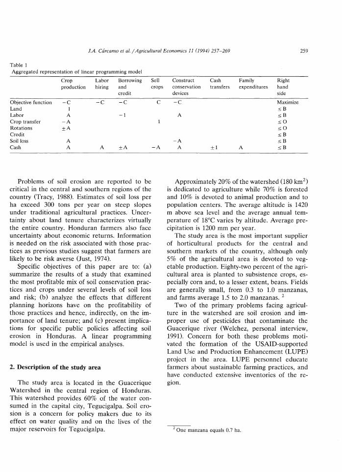
J.A. Cdrcamo et al. /Agricultural Economics 11 (1994) 257-269 259

Table 1 Aggregated representation of linear programming model

Crop Labor Borrowing Sell production hiring and crops

credit

Objective function -c -c -c Land Labor A -1 Crop transfer -A Rotations ±A Credit Soil loss A Cash A A ±A

Problems of soil erosion are reported to be critical in the central and southern regions of the country (Tracy, 1988). Estimates of soil loss per ha exceed 300 tons per year on steep slopes under traditional agricultural practices. Uncer­tainty about land tenure characterizes virtually the entire country. Honduran farmers also face uncertainty about economic returns. Information is needed on the risk associated with those prac­tices as previous studies suggest that farmers are likely to be risk averse (Just, 1974).

Specific objectives of this paper are to: (a) summarize the results of a study that examined the most profitable mix of soil conservation prac­tices and crops under several levels of soil loss and risk; (b) analyze the effects that different planning horizons have on the profitability of those practices and hence, indirectly, on the im­portance of land tenure; and (c) present implica­tions for specific public policies affecting soil erosion in Honduras. A linear programming model is used in the empirical analyses.

2. Description of the study area

The study area is located in the Guacerique Watershed in the central region of Honduras. This watershed provides 60% of the water con­sumed in the capital city, Tegucigalpa. Soil ero­sion is a concern for policy makers due to its effect on water quality and on the lives of the major reservoirs for Tegucigalpa.

c

-A

Construct Cash Family Right conservation transfers expenditures hand devices side

-c Maximize ~B

A ~B

~0

~0

~B

-A ~B

A ±1 A ~B

Approximately 20% of the watershed (180 km2 )

is dedicated to agriculture while 70% is forested and 10% is devoted to animal production and to population centers. The average altitude is 1420 m above sea level and the average annual tem­perature of 18°C varies by altitude. Average pre­cipitation is 1200 mm per year.

The study area is the most important supplier of horticultural products for the central and southern markets of the country, although only 5% of the agricultural area is devoted to veg­etable production. Eighty-two percent of the agri­cultural area is planted to subsistence crops, es­pecially corn and, to a lesser extent, beans. Fields are generally small, from 0.3 to 1.0 manzanas, and farms average 1.5 to 2.0 manzanas. 2

Two of the primary problems facing agricul­ture in the watershed are soil erosion and im­proper use of pesticides that contaminate the Guacerique river (Welchez, personal interview, 1991). Concern for both these problems moti­vated the formation of the USAID-supported Land Use and Production Enhancement (LUPE) project in the area. LUPE personnel educate farmers about sustainable farming practices, and have conducted extensive inventories of the re­gion.

2 One manzana equals 0.7 ha.

260 J.A. Carcamo eta!. 1 Agricultural Economics 11 (1994) 257-269

3. Methods and data

A representative farm model was constructed for the watershed using field survey data, enter­prise budgets, and calculations of soil loss using the Universal Soil Loss Equation (USLE) with its coefficients tailored to Honduras. The model was solved using linear programming, with an objec­tive of maximizing net returns subject to various levels of soil loss and risk. The model incorpo­rated several soil conservation practices and culti­vation methods.

A highly aggregated tableau for the base model without risk activities and constraints is presented in Table 1. The letters A, B and C represent sets of coefficients. In general, a negative sign on a coefficient in the tableau indicates that an activity supplies cash, production, labor, etc., while a positive sign indicates that a product, input, or cash is required. The presence of both a positive and a negative sign on the same coefficient indi­cates that the coefficient in the tableau repre­sents a set of coefficients on rows and activities containing poth positive and negative signs.

Major activities included crop production on three land types, labor hiring, borrowing, selling crops, construction of soil conservation devices, cash transfers, and an activity to place a mini­mum bound on family expenditures. A total of 243 activities were included. Major constraints included land, labor, crop transfers, rotations, credit, soil loss, and cash. A total of 197 con­straints were incorporated. When a risk compo­nent was added to the model, the objective func­tion was to minimize mean absolute deviations from average income for several levels of net returns and soil loss. Deviations from mean in­come from each activity were included in a set of risk constraints at the bottom of the model fol­lowing the MOTAD procedure of Hazell and Norton (1986).

Crops may be grown on land type A (2% slope), land type B (10% slope), or land type C (24% slope). There were 181 crop production activities that resulted from combinations of crops, planting seasons, land types, soil conserva­tion devices used, and tillage systems. Cropping activities used land, labor, and capital to produce

crops that were transferred and sold. Land could also be taken out of production to meet soil loss restrictions. Borrowing activities were allowed in each month at the interest rate being charged by the farmers' cooperative, the primary source of credit in the area. Borrowing supplied cash in each month and required payment with interest in subsequent months. Available family labor was 48 person-months per year.

Monthly cash requirements for productive in­puts were calculated for each crop. All such cash requirements and family expenses were paid from an initial cash endowment, crop sales, or from borrowing. Transfers of surplus cash to the subse­quent month were made each month. At the end of the year, cash had to be sufficient to repay loans and to replace the initial cash endowment. 3

Coefficients on cropping activities in the soil loss constraint specified the amount of soil loss for particular crops on each land type in each time period under different tillage practices and with different soil conservation devices. The right hand side of this constraint specified the amount of soil loss allowed for the farm.

3.1. Farmer survey

Data to generate many of the coefficients for the representative farm models were obtained by surveying farmers in the watershed during July 1991. Twelve farmers were chosen at random from the list of farmers in the region provided by the LUPE project. In each interview farmers were asked questions about the make-up of the family, land tenure, crops and rotations including pro­duction costs and output prices, soil conservation practices, labor use and costs, and credit. The length and slope of each field were measured, and the number of manzanas that fall within each

3 The cash constraint began with an endowment of 494 Lempiras (US$1.00 = 5.5 L.). Each month, 386 L. for family expenses and input expenses that varied by crop, depending on the budget and agricultural calendar, were subtracted. Sales of crops added to the cash in the month in which the sales occurred, and the household was free to borrow for consumption at the appropriate interest rate.

J.A. Ctircarno eta/. j Agricultural Economics 11 (1994) 257-269 261

slope and the crops grown on each degree of slope were recorded.

The average farm in the survey was found to have 1.7 manzanas with 35% of the area with an average slope of 2%, 26% of the area with an average slope of 10%, and 39% with an average slope of 24%.

The most important crops in the area are corn, beans, corn and beans intercropped, cabbage, onions, and tomatoes. A small amount of coffee is also produced. Production is continuous from May through December (the rainy season), and when irrigation is available it extends through the summer months of January through April. Sixty percent of the farmers have irrigation on an aver­age of 24% of the area.

The main means of conserving soil found in the survey included contour cultivation, live barri­ers, hill-side ditches, and terraces. The most com­mon tillage system found was conventional, with minimum and no-till observed on a few farms. All three tillage systems were included in the linear programming model for corn, beans, and corn­beans intercropped. Only conventional tillage was allowed in the model for cabbage, tomatoes, onions, and coffee.

The average family consisted of four people. Agricultural activities were performed to a greater degree by men and children, but women helped with agricultural activities when needed. A coop­erative in the area provided credit at an annual interest rate of 24% although only three out of the 12 farmers surveyed used credit.

3.2. Soil loss values

Soil loss values were required for each produc­tion activity. These values were incorporated into a soil loss constraint and specified the amount of soil loss that would occur under specific manage­ment practices, weather, type of soil, slope, and soil conservation devices. The USLE was used to calculate soil loss coefficients. Briefly, the USLE predicts gross soil loss per unit of land as:

A =RKLSCP

where A is the computed soil loss per unit area per unit of time, R is a rainfall and runoff factor,

K is a soil erodability factor, L is a slope length factor, S is a slope steepness factor, C is a ground cover and management factor, and P is a support practice factor. The latter is the ratio of soil loss with a device like contouring or terracing to that with straight-row farming up and down the slope.

Values for each factor were derived for the study area. The rainfall and runoff factor, R, was located in a study completed near the study area (Wouters, 1980). The soil erodability factor was calculated using information from a soil analysis in the study area (Recursos Hfdricos, 1983) and from Wischmeier and Smith (1978). Values for P, L and S were also obtained from Wischmeier and Smith except for live barriers. Values for live barriers were based on interpolated values be­tween contour cultivation and hillside ditches. The C factor is measured as the ratio of soil loss from an area with specified cover and manage­ment to that with tilled fallow. It was calculated for each combination of crop and tillage system following procedures in Wischmeier and Smith. Crop stages were identified through consultation with agronomists in the area. Cabbage, onions, and beans were the most erosive crops.

3.3. Budgets

Crop budgets were constructed and the result­ing information on input use, prices, and input costs was incorporated into the linear program­ming model. Budgets were based on those pub­lished for the Central region of Honduras and adjusted by information gathered in the farm level survey and by agronomists in the area. Yields were varied by slope. Land with 2% slope was assumed to yield 0.5% more than land with 10% slope and 3% more than land with 24% slope. These yield differences reflect only the effect of slope on the amount of horizontal land area under production and hence may be considered to be minimum differences. Other factors such as lower root depth, and poorer nutrient content are likely to reduce yields on higher sloped lands by even more; data for these adjustments do not, however, exist.

The costs of constructing and maintaining con-

262 J.A. Carcamo et al. 1 Agricultural Economics II ( I994) 257-269

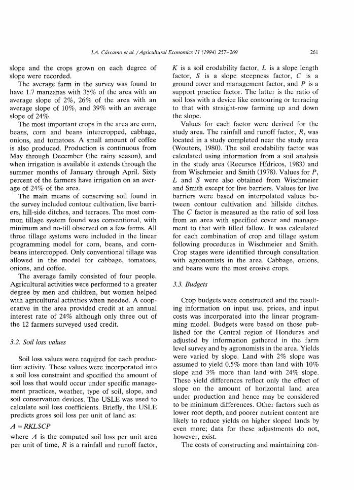
Table 2 Effects of soil loss restrictions on income, crops produced, and on conservation devices and tillage systems used

Percent Soil loss Income Percent Crop activities (manzanas) a.b Conservation device and tillage system c

soil loss (tons; (L.) slope allowed manzana)

CR BN CR-BN CB ON CF cc CM CN LC LM LN TC TM TN 100 328 5929 2 0.45 0.45 0.28 - 1.19 -

10 0.33 0.33 0.21 - 0.86 -

24 0.49 0.49 0.31 - 1.30 -80 263 5877 2 0.45 - 0.45 0.28 - 1.19 -

10 0.33 0.33 0.21 - 0.86 -24 0.48 - 0.48 0.31 - 0.84 - 0.42 -

60 197 5823 2 0.45 - 0.45 0.28 - 1.19 -10 0.33 - 0.33 0.21 - 0.86 -24 0.46 - 0.46 0.31 - 0.38 - 0.85 -

40 131 5749 2 0.45 - 0.45 0.28 - 1.19 -10 0.32 - 0.32 0.21 - 0.64 - 0.20 -24 0.46 - 0.46 0.29 - 1.21 -

20 66 5152 2 0.45 - 0.45 0.28 - 1.19 -

10 0.31 - 0.31 0.19 - 0.81 -

24 0.42 - 0.42 0.06 0.12 - 0.90 -10 33 4482 2 0.45 - 0.45 0.28 - 1.19 -

10 0.31 - 0.31 0.19 - 0.81 -

24 0.45 0.16 0.16 - 0.35 0.10 -5 16 3870 2 0.45 - 0.44 0.28 - 1.19 -

10 0.09 0.29 - 0.29 0.19 - 0.39 - 0.38 -24 0.16 0.16 -

2 7 2826 2 0.44 0.44 0.28 - 1.16 -

10 0.06 0.11 0.19 0.11 - 0.23 0.25 0.06 24

a CR, corn; BN, beans; CR-BN, corn and beans intercropped; CB, cabbage; ON, onion; CF, coffee. b The sum of areas planted exceeds the total available land area per farm due to planting in more than one season. c CC, CM, CN, contour cultivation with conventional, minimum and no tillage, respectively. LC, LM, LN, live barriers with conventional, minimum and no tillage, respectively. TC, TM, TN, terraces with conventional, minimum tillage and no tillage, respectively.

servation devices were calculated based on infor­mation in Almendariz (1990), Tracy and Mungia (1986), Michaelson (1986), and from information provided by LUPE personnel. These costs, which were composed entirely of hired labor expenses, were averaged over a 10-year planning horizon; the practices were assumed to have a 10-year life. Thus, one tenth of the total construction labor and a 10% annual maintenance allowance were charged for each conservation device in the an­nual model. Inclusion of conservation devices also required calculation of their effects on the amount of land available to cultivate. The amount of land removed from production by the presence of these devices (such as grass strips, etc.) on steep slopes is considerable.

Risk was included in the model by gathering 5 years of average yield data from various sources 4

and crop prices (retail) from a publication of the Unidad de Planificaci6n Sectorial Agricola (1990). Thus, both yield and price risk were included in the measurement of income risk in the model.

A one-year linear programming model that maximizes net farm income was used to examine the effects of different soil loss levels on farm income. The one-year model may be considered to be an average year when the farmer is in an equilibrium state. A MOTAD model that mini-

4 The sources included Gonzales Rey et a!. (1991), FAO (1990) and Unidad de Planificaci6n Sectorial Agricola (1990).

J.A. Carcamo et al. 1 Agricultural Economics 11 (1994) 257-269 263

mizes ·deviations in income from average income was used to assess risk levels when income and/or soil loss restrictions were imposed.

4. Results

Four sets of analyses were completed with the linear programming model: (a) income-soil loss tradeoffs, (b) risk-income tradeoffs, (c) considera­tion of the effects of varying the length of plan­ning horizon, and (d) an analysis of the optimal level of soil loss given a range of assumptions about the effect of erosion reduction on average yields. The result of these analyses are presented below with interpretation of selected shadow

Table 3

prices and description of some of the sensitivity analysis performed.

4.1. Income-soil loss tradeoffs

The effects of different soil loss limits on net farm income, crops produced, and on conserva­tion devices and tillage systems are presented in Table 2. With no limit on soil loss, 328 tons of soil per manzana per year would be lost (this amount is called the base loss) and a net income of 5929 L. (this is equivalent to US$1078) would be earned on the representative farm. More than a 50% reduction in soil erosion can be achieved with little effect on income. However, when soil loss is restricted to 20% or less of the initial base

Solutions to linear programming model when net income risk is minimized subject to a series of income levels but soil loss is unconstrained

Income Income Soil loss Percent Crop activities (manzanas) a

(L.) variance h (tonsjmanzana) slope CR BN CR-BN CB ON (thousand)

5929.24 2020 328.24 2 0.45 0.45 0.28 10 0.33 0.33 0.21 24 0.49 0.49 0.31

5876.92 1833 325.44 2 0.45 0.45 0.28 10 0.33 0.33 0.21 24 0.54 0.54 0.21

5824.61 1655 322.64 2 0.45 0.45 0.28 10 0.33 0.33 0.21 24 0.59 0.59 0.11

5748.80 1418 319.43 2 0.45 0.45 0.28 10 0.34 0.34 0.17 24 0.65 0.65

5152.02 486 250.60 2 0.10 0.38 0.10 0.48 0.02 10 0.10 0.22 0.10 0.32 24 0.16 0.34 0.16 0.49

4482.37 282 184.11 2 0.17 0.28 0.14 0.43 10 0.12 0.21 0.10 0.31 24 0.48 0.11 0.06 0.17

3869.75 120 144.24 2 0.17 0.28 0.14 0.43 10 0.27 0.10 0.05 0.14 24 0.65

2825.81 3 138.07 2 0.53 0.03 0.04 0.04 10 0.43 24 0.65

a See Table 2 for definitions. b Calculated as M 2[ 7Ttj2(t- 1)], where M is the mean absolute deviation of expected income, 7T is the mathematical constant 22/7, and t is the number of yearly risk constraints, in this case 5.

264 J.A. Carcamo et al. 1 Agricultural Economics 11 (1994) 257-269

loss, income drops more sharply. If only 2% of the quantity of soil loss under no restrictions is allowed (7 tons per manzana per year), income is reduced to 2826 L. 5

Bean, cabbage, and onion production under conventional tillage and contour cultivation lead to the highest income and greatest soil loss. Bor­rowing occurs only in May and labor is not hired. Soil loss restrictions have little effect on the mix of crops grown until only 20% of the base soil loss is allowed. At that point, coffee is grown on the steepest slopes. When only 2% of the base soil loss is permitted, the steepest slopes are left uncultivated.

Conventional tillage with contour cultivation predominates, but as erosion restrictions are tightened, first live barriers with conventional tillage and later terraces with conventional tillage enter the solution. With only 10% of the initial soil loss allowed, live barriers with minimum tillage come in, and at 2% soil loss allowed, terraces combined with minimum and no-till en­ter the solution. Hillside ditches never enter the solution because they are roughly as effective as live barriers in reducing erosion but cost more to construct. Income levels drop when lower amounts of soil loss are allowed because of the cost involved in constructing conservation de­vices, the shifts in crop mix, and the land re­moved from production at very restrictive levels of soil loss.

4.2. Risk-income tradeoffs

The effects of erosion reduction strategies on the risk-return tradeoff faced by farmers were analyzed under two scenarios. In the first, risk was minimized subject to different levels of in­come with no constraint on the amount of soil loss. In the second, risk was minimized subject to the income and erosion levels in Table 2. The results of the analysis for the unconstrained soil loss scenario are summarized in Table 3 with

5 Average per capita income in Honduras in 1989 was 4950 L.

Income (L./year) (Thousands) 7

6

5

4

3

2

Soil Loss

-Unconstrained

+constrained

0~----~------~------~----~------~

0 500 1000 1500 2000 2500

Variance (1000 of L.)

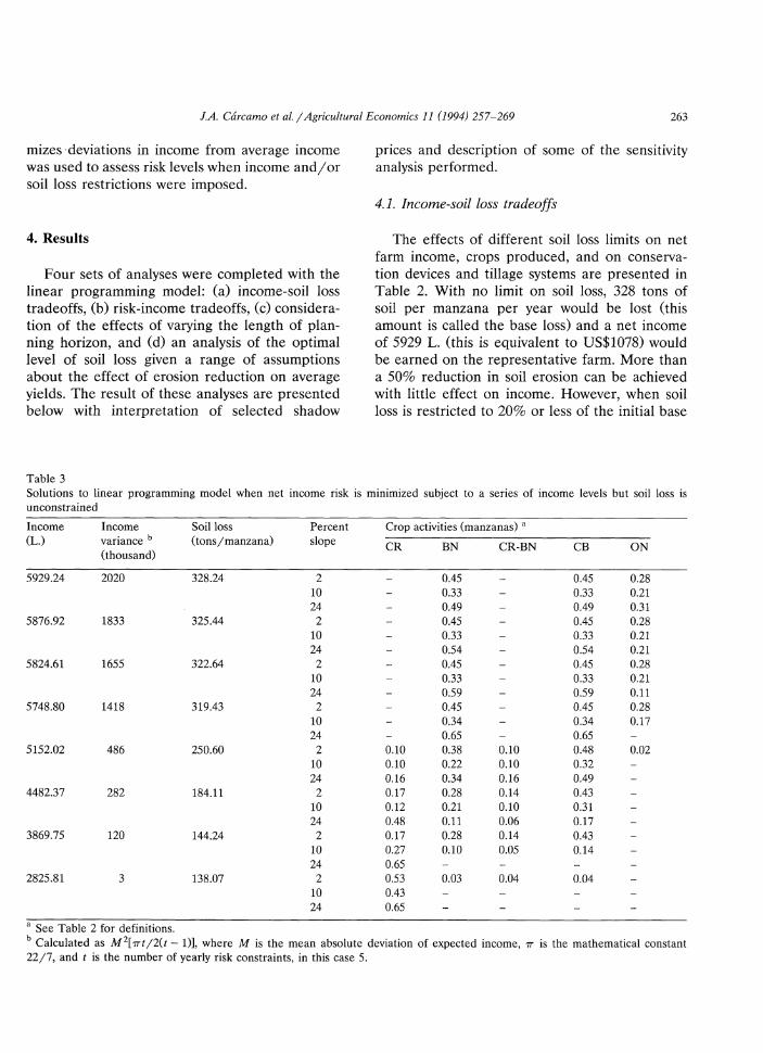
Fig. 1. Income-variance tradeoff.

respect to income levels, soil loss, and cropping activities.

Income and risk are positively related and thus as risk is reduced, so too is income. Soil loss declines with income and risk, but of course higher levels of soil loss are associated with any particular level of income when soil loss is uncon­strained compared to the case when soil loss is constrained. When risk is minimized, beans and cabbage enter the solution at every income level whereas corn and beans-corn intercropped enter only at lower levels of income and risk (compare Tables 2 and 3). Onions enter only at higher levels of income and risk. Under this scenario with no soil loss restrictions, erosion control de­vices are not constructed. Hence, all changes in soil loss are due to differences in cropping activi­ties.

Expected income and variance (EV) frontiers were constructed for (a) the scenario in which risk was minimized for several levels of income but soil loss was not restricted and (b) the sce­nario in which risk was minimized and both in­come and soil loss were constrained (Fig. 1). These EV frontiers illustrate that there is sub­stantially more risk encountered when achieving the constrained level of soil loss. Because most studies have found farmers to be risk averse, this implies that mechanisms for reducing price and yield risk may be needed to provide additional incentives for soil conservation. Crop insurance

J.A. Cdrcamo et al. /Agricultural Economics 11 (1994) 257-269 265

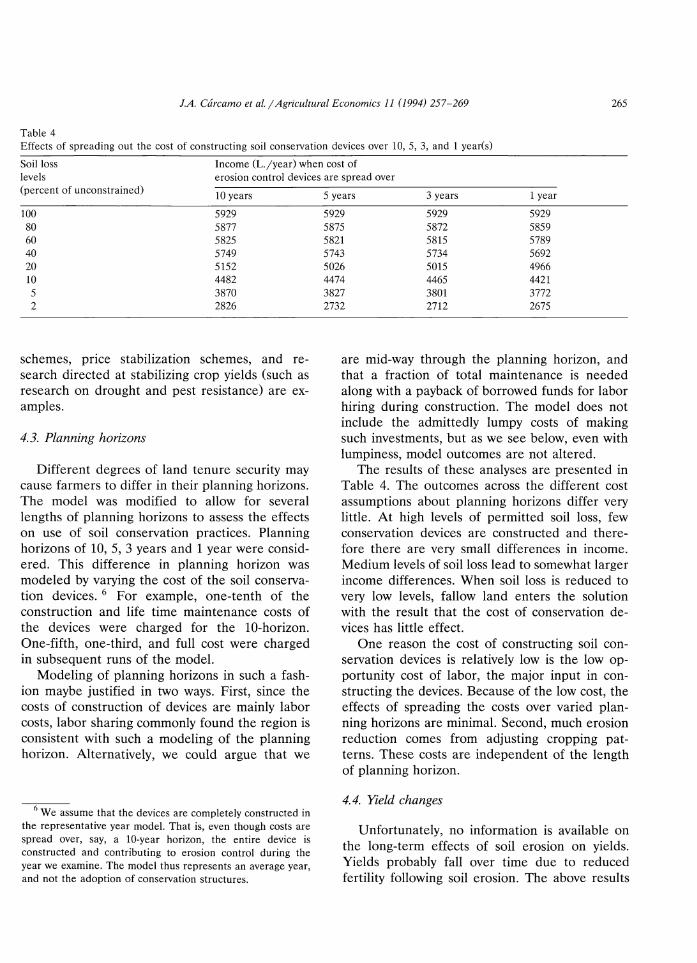
Table 4 Effects of spreading out the cost of constructing soil conservation devices over 10, 5, 3, and 1 year(s)

Soil loss Income (L.jyear) when cost of levels erosion control devices are spread over (percent of unconstrained) 10 years

100 5929 80 5877 60 5825 40 5749 20 5152 10 4482 5 3870 2 2826

schemes, price stabilization schemes, and re­search directed at stabilizing crop yields (such as research on drought and pest resistance) are ex­amples.

4.3. Planning horizons

Different degrees of land tenure security may cause farmers to differ in their planning horizons. The model was modified to allow for several lengths of planning horizons to assess the effects on use of soil conservation practices. Planning horizons of 10, 5, 3 years and 1 year were consid­ered. This difference in planning horizon was modeled by varying the cost of the soil conserva­tion devices. 6 For example, one-tenth of the construction and life time maintenance costs of the devices were charged for the 10-horizon. One-fifth, one-third, and full cost were charged in subsequent runs of the model.

Modeling of planning horizons in such a fash­ion maybe justified in two ways. First, since the costs of construction of devices are mainly labor costs, labor sharing commonly found the region is consistent with such a modeling of the planning horizon. Alternatively, we could argue that we

6 We assume that the devices are completely constructed in the representative year model. That is, even though costs are spread over, say, a 10-year horizon, the entire device is constructed and contributing to erosion control during the year we examine. The model thus represents an average year, and not the adoption of conservation structures.

5 years 3 years 1 year

5929 5929 5929 5875 5872 5859 5821 5815 5789 5743 5734 5692 5026 5015 4966 4474 4465 4421 3827 3801 3772 2732 2712 2675

are mid-way through the planning horizon, and that a fraction of total maintenance is needed along with a payback of borrowed funds for labor hiring during construction. The model does not include the admittedly lumpy costs of making such investments, but as we see below, even with lumpiness, model outcomes are not altered.

The results of these analyses are presented in Table 4. The outcomes across the different cost assumptions about planning horizons differ very little. At high levels of permitted soil loss, few conservation devices are constructed and there­fore there are very small differences in income. Medium levels of soil loss lead to somewhat larger income differences. When soil loss is reduced to very low levels, fallow land enters the solution with the result that the cost of conservation de­vices has little effect.

One reason the cost of constructing soil con­servation devices is relatively low is the low op­portunity cost of labor, the major input in con­structing the devices. Because of the low cost, the effects of spreading the costs over varied plan­ning horizons are minimal. Second, much erosion reduction comes from adjusting cropping pat­terns. These costs are independent of the length of planning horizon.

4.4. Yield changes

Unfortunately, no information is available on the long-term effects of soil erosion on yields. Yields probably fall over time due to reduced fertility following soil erosion. The above results

266 J.A. Carcamo et al. j Agricultural Economics 11 (1994) 257-269

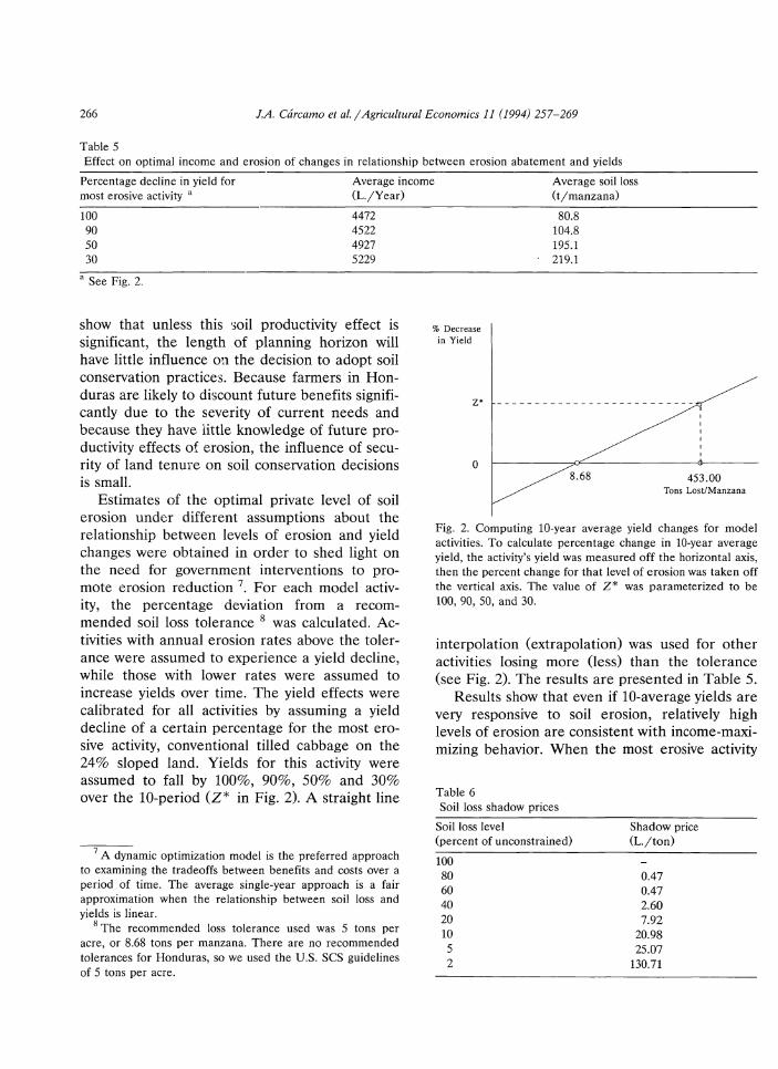
Table 5 Effect on optimal income and erosion of changes in relationship between erosion abatement and yields

Percentage decline in yield for most erosive activity a

100 90 50 30

a See Fig. 2.

Average income (L.jYear)

4472 4522 4927 5229

Average soil loss (tjmanzana)

80.8 104.8 195.1 219.1

show that unless this soil productivity effect is significant, the length of planning horizon will have little influence on the decision to adopt soil conservation practices. Because farmers in Hon­duras are likely to discount future benefits signifi­cantly due to the severity of current needs and because they have little knowledge of future pro­ductivity effects of erosion, the influence of secu­rity of land tenure on soil conservation decisions is small.

% Decrease in Yield

Estimates of the optimal private level of soil erosion under different assumptions about the relationship between levels of erosion and yield changes were obtained in order to shed light on the need for government interventions to pro­mote erosion reduction 7. For each model activ­ity, the percentage deviation from a recom­mended soil loss tolerance 8 was calculated. Ac­tivities with annual erosion rates above the toler­ance were assumed to experience a yield decline, while those with lower rates were assumed to increase yields over time. The yield effects were calibrated for all activities by assuming a yield decline of a certain percentage for the most ero­sive activity, conventional tilled cabbage on the 24% sloped land. Yields for this activity were assumed to fall by 100%, 90%, 50% and 30% over the 10-period (Z* in Fig. 2). A straight line

7 A dynamic optimization model is the preferred approach to examining the tradeoffs between benefits and costs over a period of time. The average single-year approach is a fair approximation when the relationship between soil loss and yields is linear.

8 The recommended loss tolerance used was 5 tons per acre, or 8.68 tons per manzana. There are no recommended tolerances for Honduras, so we used the U.S. SCS guidelines of 5 tons per acre.

Z* ------ - --- -- - ------ -

0 453.00

Tons Lost/Manzana

Fig. 2. Computing 10-year average yield changes for model activities. To calculate percentage change in 10-year average yield, the activity's yield was measured off the horizontal axis, then the percent change for that level of erosion was taken off the vertical axis. The value of Z* was parameterized to be 100, 90, 50, and 30.

interpolation (extrapolation) was used for other activities losing more (less) than the tolerance (see Fig. 2). The results are presented in Table 5.

Results show that even if 10-average yields are very responsive to soil erosion, relatively high levels of erosion are consistent with income-maxi­mizing behavior. When the most erosive activity

Table 6 Soil loss shadow prices

Soil loss level (percent of unconstrained)

100 80 60 40 20 10 5 2

Shadow price (L.jton)

0.47 0.47 2.60 7.92

20.98 25.07

130.71

J.A. Carcamo eta/. I Agricultural Economics 11 (1994) 257-269 267

Table 7 Effect on farm income of changing crop prices and labor costs

Soil loss Base Income (L.) (tonjmanzana) income 10% change

level in vegetable prices

Increase Decrease

328 5929 6974 4884 363 5877 6913 4840 197 5825 6854 4796 131 5749 6762 4735 66 5152 6027 4311 33 4482 5113 3851 16 3870 4491 3253 7 2826 3285 2414

is assumed to lose 100% of its yield over a 10-period, income falls to 4472 L. per year and 'optimal' erosion is 80.8 tons per manzana. If yields are less responsive to erosion levels, in­come falls by less and erosion increases. When yields for the most erosive activity fall by only 30% over the 10-period, income averages 5229 L. per year, with an annual erosion level of 219.1 tons per manzana.

When erosion rates affect yields, a consistent pattern emerges. Soil conservation devices are constructed on the less steeply-sloped land (first live barriers and, as yields become more respon­sive, terraces), while rotation changes occur on the less steeply-sloped land. As yield declines caused by erosion become progressively larger, the 24% sloped land is gradually taken out of production. The high rates of erosion that occur on the steeper slopes mean that production there is unsustainable over time, though productivity actually grows (through soil conservation) on the less steeply-sloped lands.

If information on yield responses were avail­able 9 the results could be used to provide a measure of optimal soil loss from the farmers' perspective. Given the high levels of 'optimal erosion' from this analysis and the high off-farm costs associated with erosion, it is clear that there

9 No information from Honduras was available. As an ex­ample, Burt used a response elasticity of 0.33 in his investiga­tion of soil loss in Washington state.

15% change in 10% percent change in corn and bean prices coffee prices

Increase Decrease Increase Decrease

6325 5533 5929 5929 6268 5486 5871 5877 6210 5439 5825 5825 6132 5366 5749 5749 5519 4785 5197 5109 4854 4119 4538 4426 4125 3637 3926 3814 3092 2608 2826 2825

is a need for government action to promote re­duced erosion. If yields are very responsive to erosion the private decision-maker will reduce erosion to 80.8 tons per manzana per year, yet this level is still likely to create significant off-farm damages, and soil productivity on the steeply­sloped lands will fall dramatically over the ten­year period. Incentives need to be provided to increase the rates of conservation on more steeply-sloped lands.

4.5. Shadow prices and sensitivity analysis

Shadow prices were calculated for different levels of soil loss allowed, using the model with­out the risk component (Table 6). These shadow prices represent the amount by which the objec­tive function would change if the constraint on soil loss were changed by one unit. They repre­sent the cost of erosion reductions. The value of 0.47 associated with high levels of erosion means that the marginal value of an extra ton of soil loss is 0.47 L. The value associated with changing the soil loss restriction when only 10% is allowed is 20.98 L. Thus as progressively less erosion is permitted, the cost of additional reductions in­creases.

Sensitivity analysis was also performed on sev­eral prices and on wages (Table 7). This analysis is useful for assessing the sensitivity of the opti­mal solution to changes in policies that might influence these prices. Vegetable prices were changed 10% (higher and lower), corn and beans

268 J.A. Carcamo eta!. j Agricultural Economics 11 (1994) 257-269

were changed 15%, and coffee was changed 10%. 10 Farm income was more sensitive to changes in vegetable prices than to changes in prices of corn, beans, or coffee. Soil conservation is facilitated as vegetable prices fall because veg­etables are generally more erosive than other crops. Coffee price changes have little effect on income as relatively little coffee is grown even if the price rises 10%. Increasing wages by 25% has only a slight effect on income.

5. Conclusions and implications

This paper has examined the economic incen­tives for farmers to plant particular crops, use alternative tillage practices, and construct soil erosion devices under increasing restrictions on soil loss allowed and alternative levels of risk. The results indicate that considerable reductions in soil. loss can be achieved, primarily through altering cropping patterns. Substantial reductions in the very high rates of erosion found can only be achieved at significant cost to the farmer. Because of the high off-farm costs associated with these erosion rates, providing better information to the farmer will not, in isolation, lead to erosion rates that are compatible with socially optimal levels. If erosion is reduced from 328 tons per manzana per year to 7 tons per year, income would be lowered from 5929 to 2826 L. However, more than a 50% reduction in soil loss can be achieved at relatively little loss of income. Cab­bage and onions, the highest-return crops, are also the most erosive and were always present in the farm plans regardless of the levels of soil loss required. The lowest levels of soil erosion were achieved when some land was removed from pro­duction.

Higher income plans were riskier regardless of the level of soil loss. However, reduced soil loss was achieved at the cost of higher risk. Hence risk may be a significant barrier to wider use of soil erosion practices in the watershed.

10 We examine changes in relative prices only; changes in the overall price level will have a proportionate impact on income and, thus, are not examined.

Relatively small differences in income were found when the cost of constructing soil conser­vation devices was spread over several years rather than just one year. This small difference suggests that insecure tenure may not be a significant barrier to adoption of these devices. Hence, in­centive packages designed to promote construc­tion of these devices may be effective regardless of tenure status. Because most of the soil erosion occurred on the more steeply-sloped lands and because the model never constructed erosion control devices on the steeply-sloped lands, spe­cial attention needs to be devoted to them. Incen­tives should be provided either to take these lands out of production (e.g., creation of perma­nent pasture) or to promote erosion control there.

Government intervention is needed to pro­mote less erosive practices. Even if it is assumed that yields are very responsive to erosion, high levels of erosion are optimal from a private deci­sionmaker's perspective. External costs of such rates are likely to be excessive, so that action to internalize the costs is necessary.

The assumption of constant technical coeffi­cients over a 10-planning horizon may be unreal­istic. As soil is lost, the production relationships change over time, and new technologies may also vary these relationships. Innovations that make it easier to conserve soil, including better ground cover, wider root bases, and more quickly-devel­oping plant varieties may benefit these farmers. It is clear that the cost to the farmer of conserving is excessive under current technologies, and im­proved conservation techniques are needed to achieve the twin goals of conserving soil and maintaining farm incomes. The innovations de­scribed above may also lower yield risk.

Some other policy implications of this study are that the government may want to provide incentives to farmers to target steeper slopes for coffee, intermediate slopes for corn and beans and flatter areas for vegetables. These incentives might be in the form of restrictions on particular cropping practices or price policies. It appears that live barriers and minimum tillage should be encouraged by the extension service. Policies to reduce income risk may also encourage soil con­servation. Crop insurance, irrigation projects,

J.A. Carcarno et al. j Agricultural Economics 11 (1994) 257-269 269

price stabilization schemes, or research to de­velop more drought- and pest-resistant crop vari­eties are examples.

References

Almendariz, R., 1990. Estimaci6n de Rendimientos y Costos de Zanjas de Ladera en Suelos de Ia Cuenca del Rio Bonito La Ceiba, Athintida. Tesis de Ingeniero Agr6nomo, Centro Universitario Regional del Litoral Atlantico, La Ceiba, Honduras.

Anderson, J.R. and J. Thampapillai, 1990. Soil conservation in developing countries: project and policy intervention. Policy and Research Series 8, World Bank, Washington, DC.

Barbier, E.B., 1990. The farm-level economics of soil conser­vation: the uplands of Java. Land Econ., 66: 199-211.

Binswanger, H.P., 1980. Attitudes toward risk: experimental measurement in rural India. Am. J. Agric. Econ., 62 (May): 395-407.

Blase, M.G., 1960. Soil erosion control in western Iowa: progress and problems. Ph.D. dissertation, Iowa State University, Ames.

Boggess, W.J., J. McGrann, M. Boehlje and E.O. Heady, 1979. Farm level impacts of alternative soil loss control policies. J. Soil Water Conserv., 34: 177-183.

Erwin, D.E. and R.A. Washburn, 1981. Profitability and soil conservation practices in Missouri. J. Soil Water Conserv., 36: 107-111.

FAO, 1990. 1990 Production Yearbook. Food and Agricul­tural Organization of the United Nations, Rome.

Feder, G. and T. Onchan, 1987. Land ownership security and farm investment in Thailand. Am. J. Agric. Econ., 69: 311-320.

Gonzales-Rey, D., M. L6pez-Pereira and J.H. Sanders, 1991. The impact of new sorghum cultivars and other associated technologies in Honduras. INTSORMIL Project, Teguci-galpa, Honduras. ·

Hazell, P. and R. Norton, 1986. Mathematical Programming For Economic Analysis in Agriculture. Macmillan, New York.

Just, R.E., 1974. An investigation of the importance of risk in farmers' decisions. Am. J. Agric. Econ., 56:14-25.

Kramer, R.A., W.T. McSweeney and R.W. Stavros, 1983. Soil Conservation with Uncertain Revenues and Input Sup­plies. Am. J. Agric. Econ., 65: 694-702.

Lee, L.K. 1980. The impact of landownership factors on soil conservation. Am. J. Agric. Econ., 63: 1070-1076.

Michaelson, T., 1986. Manual Practico de Conservaci6n de Suelos para Tierras de Ladera. Ordenaci6n Integrada de Cuencas Hidrograficas. Documento de Trabajo 3, CO­HDEFORjPNUD jFAO-HON /77 j006, Tegucigalpa, Honduras.

Recursos Hidricos, 1983. Estudio de Suelos a Reconocimiento de las Cabeceras del Rio Choluteca. Tegucigalpa, Hon­duras.

Repetto, R., 1989. Economic incentives for sustainable pro­duction. In: G. Schramm and J. Warford (Editors) Envi­ronmental Management and Economic Development. Johns Hopkins University Press, Baltimore, MD.

Seitz, W.D., C.R. Taylor, R.G.F. Spitze, C. Osteen and M.C. Nelson, 1979. Economic impacts of soil erosion control. Land Econ., 55: 28-42.

Tracy, F.C., 1988. The natural resource management project in Honduras. In: W.C. Moldenhauer and N.W. Hudson (Editors) Conservation Farming on Steep Lands. Soil and Water Conservation Society, USA.

Tracy, F. and P. Mungia, 1986. Manual practico de conserva­ci6n de suelos. Proyecto Manejo de Recursos Naturales, USAID Proyecto 522-0168, Tegucigalpa, Honduras.

Unidad de Planificaci6n Sectorial Agricola, 1990. Compendio Estadistico Agropecuario. Secretaria de Recursos Natu­rales, Tegucigalpa.

VanVuuren, W., 1986. Soil erosion: the case for market intervention. Can. J. Agric. Econ., 33: 41-62.

Veloz, A., D. Southgate, F. Hitzhusen and R. Macgregor, 1985. The economics of soil erosion control in a subtropi­cal watershed. Land Econ. 61: 145-155.

Walker, D.J., 1982. A damage function to evaluate erosion control economics. Am. J. Agric. Econ. 64: 690-698.

Walker, D.J. and J.F. Timmons, 1980. Cost of alternative policies for controlling agricultural soil loss and associated stream sedimentation. J. Soil Water Conserv., 35: 177-183.

Walker, D.J. and D.L. Young, 1986. The effects of technical progress on erosion damage and economic incentives for soil conservation. Land Econ., 62: 83-93.

Welchez, L. personal Interview, LUPE Project, August 1991. White, G.H. and E.J. Partenheimer, 1980. Economic impacts

of erosion and sedimentation control plans: case studies for pennsylvania dairy farms. J. Soil Water Conserv., 35: 76-78.

Wischmeier, W.H. and D.D. Smith, 1978. Predicting Rainfall Erosion Losses -A guide to Conservation Planning. USDA Agricultural Handbook 537, Washington, DC.

Wouters, R., 1980. Resultados de un Proyecto de Investigaci6n de Ia Erosion en Ia Cuenca Los Laureles. Corporaci6n Hondurena de Desarrollo Forestal, Tegucigalpa, Hon­duras.