On Rolling Cube Puzzles

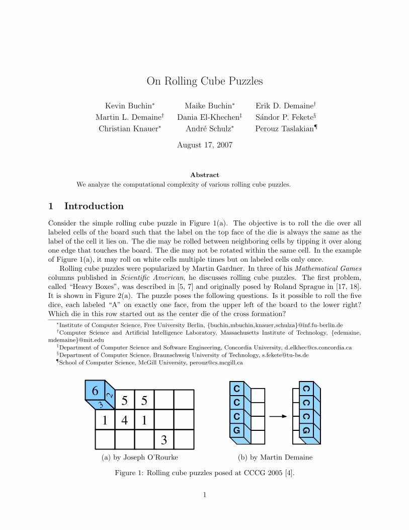
Kevin Buchin∗ Maike Buchin∗ Erik D. Demaine†

Martin L. Demaine† Dania El-Khechen‡ Sandor P. Fekete§

Christian Knauer∗ Andre Schulz∗ Perouz Taslakian¶

August 17, 2007

AbstractWe analyze the computational complexity of various rolling cube puzzles.

1 Introduction

Consider the simple rolling cube puzzle in Figure 1(a). The objective is to roll the die over alllabeled cells of the board such that the label on the top face of the die is always the same as thelabel of the cell it lies on. The die may be rolled between neighboring cells by tipping it over alongone edge that touches the board. The die may not be rotated within the same cell. In the exampleof Figure 1(a), it may roll on white cells multiple times but on labeled cells only once.

Rolling cube puzzles were popularized by Martin Gardner. In three of his Mathematical Gamescolumns published in Scientific American, he discusses rolling cube puzzles. The first problem,called “Heavy Boxes”, was described in [5, 7] and originally posed by Roland Sprague in [17, 18].It is shown in Figure 2(a). The puzzle poses the following questions. Is it possible to roll the fivedice, each labeled “A” on exactly one face, from the upper left of the board to the lower right?Which die in this row started out as the center die of the cross formation?

∗Institute of Computer Science, Free University Berlin, buchin,mbuchin,knauer,schulza@inf.fu-berlin.de†Computer Science and Artificial Intelligence Laboratory, Massachusetts Institute of Technology, edemaine,

mdemaine@mit.edu‡Department of Computer Science and Software Engineering, Concordia University, d elkhec@cs.concordia.ca§Department of Computer Science, Braunschweig University of Technology, s.fekete@tu-bs.de¶School of Computer Science, McGill University, perouz@cs.mcgill.ca

54 1

5

31

63

2

(a) by Joseph O’Rourke (b) by Martin Demaine

Figure 1: Rolling cube puzzles posed at CCCG 2005 [4].

1

(a) Heavy Boxes (b) Red-Faced Cube (c) Single Vacancy Problem

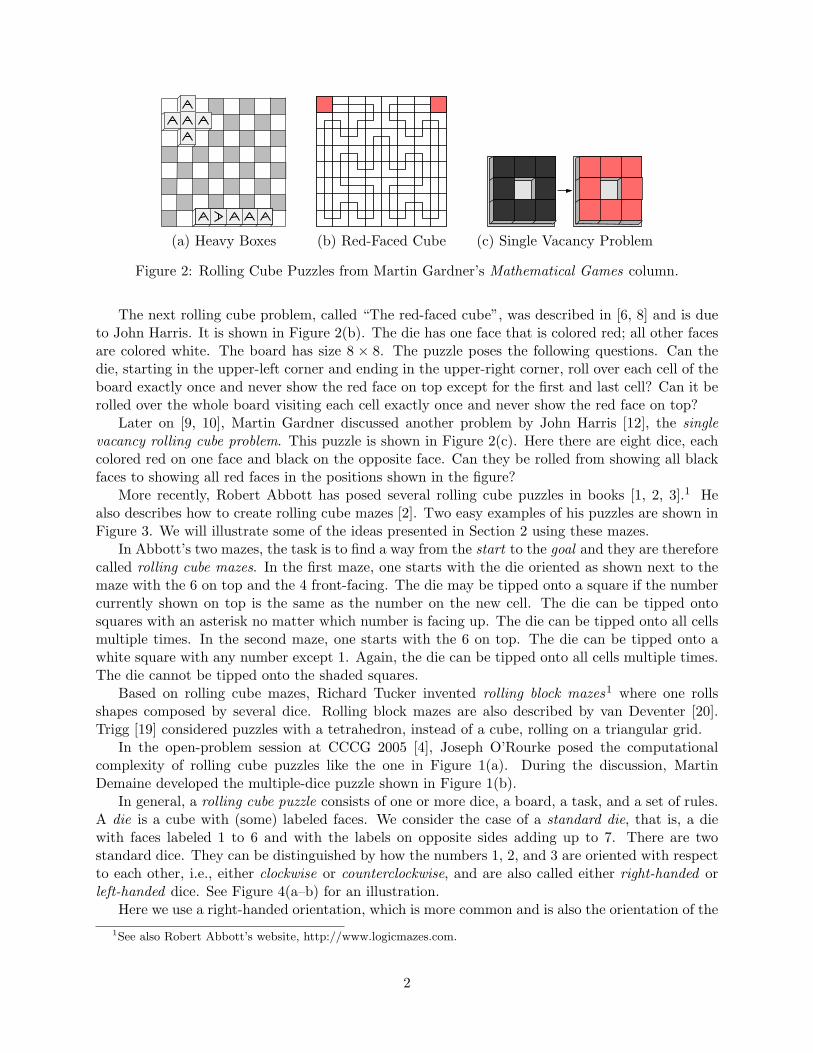
Figure 2: Rolling Cube Puzzles from Martin Gardner’s Mathematical Games column.

The next rolling cube problem, called “The red-faced cube”, was described in [6, 8] and is dueto John Harris. It is shown in Figure 2(b). The die has one face that is colored red; all other facesare colored white. The board has size 8 × 8. The puzzle poses the following questions. Can thedie, starting in the upper-left corner and ending in the upper-right corner, roll over each cell of theboard exactly once and never show the red face on top except for the first and last cell? Can it berolled over the whole board visiting each cell exactly once and never show the red face on top?

Later on [9, 10], Martin Gardner discussed another problem by John Harris [12], the singlevacancy rolling cube problem. This puzzle is shown in Figure 2(c). Here there are eight dice, eachcolored red on one face and black on the opposite face. Can they be rolled from showing all blackfaces to showing all red faces in the positions shown in the figure?

More recently, Robert Abbott has posed several rolling cube puzzles in books [1, 2, 3].1 Healso describes how to create rolling cube mazes [2]. Two easy examples of his puzzles are shown inFigure 3. We will illustrate some of the ideas presented in Section 2 using these mazes.

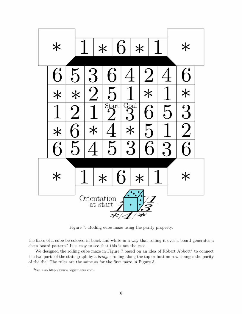
In Abbott’s two mazes, the task is to find a way from the start to the goal and they are thereforecalled rolling cube mazes. In the first maze, one starts with the die oriented as shown next to themaze with the 6 on top and the 4 front-facing. The die may be tipped onto a square if the numbercurrently shown on top is the same as the number on the new cell. The die can be tipped ontosquares with an asterisk no matter which number is facing up. The die can be tipped onto all cellsmultiple times. In the second maze, one starts with the 6 on top. The die can be tipped onto awhite square with any number except 1. Again, the die can be tipped onto all cells multiple times.The die cannot be tipped onto the shaded squares.

Based on rolling cube mazes, Richard Tucker invented rolling block mazes1 where one rollsshapes composed by several dice. Rolling block mazes are also described by van Deventer [20].Trigg [19] considered puzzles with a tetrahedron, instead of a cube, rolling on a triangular grid.

In the open-problem session at CCCG 2005 [4], Joseph O’Rourke posed the computationalcomplexity of rolling cube puzzles like the one in Figure 1(a). During the discussion, MartinDemaine developed the multiple-dice puzzle shown in Figure 1(b).

In general, a rolling cube puzzle consists of one or more dice, a board, a task, and a set of rules.A die is a cube with (some) labeled faces. We consider the case of a standard die, that is, a diewith faces labeled 1 to 6 and with the labels on opposite sides adding up to 7. There are twostandard dice. They can be distinguished by how the numbers 1, 2, and 3 are oriented with respectto each other, i.e., either clockwise or counterclockwise, and are also called either right-handed orleft-handed dice. See Figure 4(a–b) for an illustration.

Here we use a right-handed orientation, which is more common and is also the orientation of the1See also Robert Abbott’s website, http://www.logicmazes.com.

2

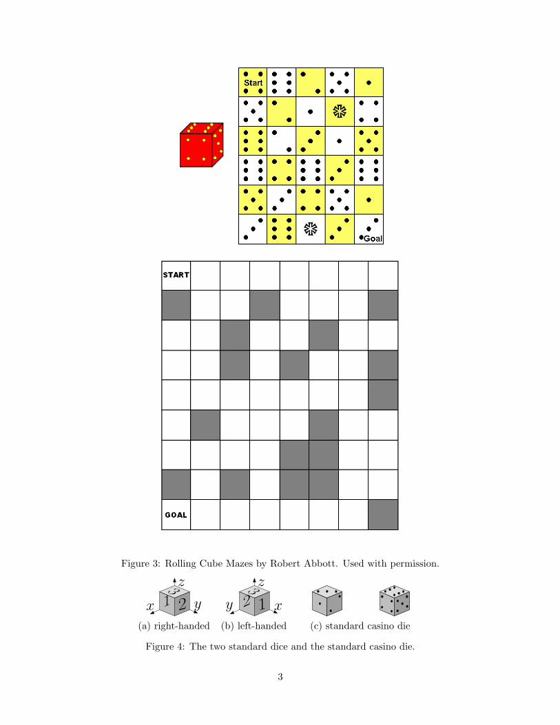
Figure 3: Rolling Cube Mazes by Robert Abbott. Used with permission.

1 23 z

yx 2 13 z

xy

(a) right-handed (b) left-handed (c) standard casino die

Figure 4: The two standard dice and the standard casino die.

3

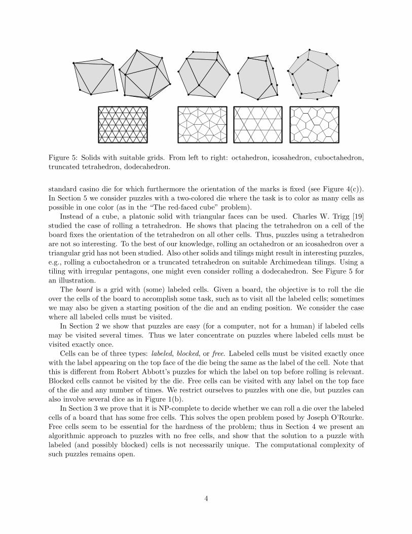
Figure 5: Solids with suitable grids. From left to right: octahedron, icosahedron, cuboctahedron,truncated tetrahedron, dodecahedron.

standard casino die for which furthermore the orientation of the marks is fixed (see Figure 4(c)).In Section 5 we consider puzzles with a two-colored die where the task is to color as many cells aspossible in one color (as in the “The red-faced cube” problem).

Instead of a cube, a platonic solid with triangular faces can be used. Charles W. Trigg [19]studied the case of rolling a tetrahedron. He shows that placing the tetrahedron on a cell of theboard fixes the orientation of the tetrahedron on all other cells. Thus, puzzles using a tetrahedronare not so interesting. To the best of our knowledge, rolling an octahedron or an icosahedron over atriangular grid has not been studied. Also other solids and tilings might result in interesting puzzles,e.g., rolling a cuboctahedron or a truncated tetrahedron on suitable Archimedean tilings. Using atiling with irregular pentagons, one might even consider rolling a dodecahedron. See Figure 5 foran illustration.

The board is a grid with (some) labeled cells. Given a board, the objective is to roll the dieover the cells of the board to accomplish some task, such as to visit all the labeled cells; sometimeswe may also be given a starting position of the die and an ending position. We consider the casewhere all labeled cells must be visited.

In Section 2 we show that puzzles are easy (for a computer, not for a human) if labeled cellsmay be visited several times. Thus we later concentrate on puzzles where labeled cells must bevisited exactly once.

Cells can be of three types: labeled, blocked, or free. Labeled cells must be visited exactly oncewith the label appearing on the top face of the die being the same as the label of the cell. Note thatthis is different from Robert Abbott’s puzzles for which the label on top before rolling is relevant.Blocked cells cannot be visited by the die. Free cells can be visited with any label on the top faceof the die and any number of times. We restrict ourselves to puzzles with one die, but puzzles canalso involve several dice as in Figure 1(b).

In Section 3 we prove that it is NP-complete to decide whether we can roll a die over the labeledcells of a board that has some free cells. This solves the open problem posed by Joseph O’Rourke.Free cells seem to be essential for the hardness of the problem; thus in Section 4 we present analgorithmic approach to puzzles with no free cells, and show that the solution to a puzzle withlabeled (and possibly blocked) cells is not necessarily unique. The computational complexity ofsuch puzzles remains open.

4

2 Basic Properties

2.1 State Graph

The state graph has a vertex for each possible state of the die and an edge for each possible transitionbetween two states. A state consists of a board position and the entire orientation of the die. Inparticular, the state encodes which label is on the top face, but even fixing this top label, there arefour possible orientations, defined by the label facing a fixed side of the board.

We will denote these orientations as xy where x is the label on the top of the die and y the labelon the back face (i.e., the side facing the top of the page in this paper). For example, in the firstmaze in Figure 3, the die starts in the state 63, because 3 is on the opposite side of the front 4.

An edge of the state graph connects vertices corresponding to adjacent cells on the board forwhich it is possible to roll a die from one cell to the other, respecting the orientations of the twostates. (Moves are reversible, so the graph is undirected.)

2.2 Parity Property

An important property of the state graph is that its vertex set naturally falls into two parts ofequal size with no edges between the two parts. For a labeled cell, only two of the four orientationsneed to be considered if we restrict the die to one part of the state graph. This corresponds tothe parity property of rolling cube puzzles [5, 12, 17, 18] which gives the solution to the puzzle inFigure 2(a).

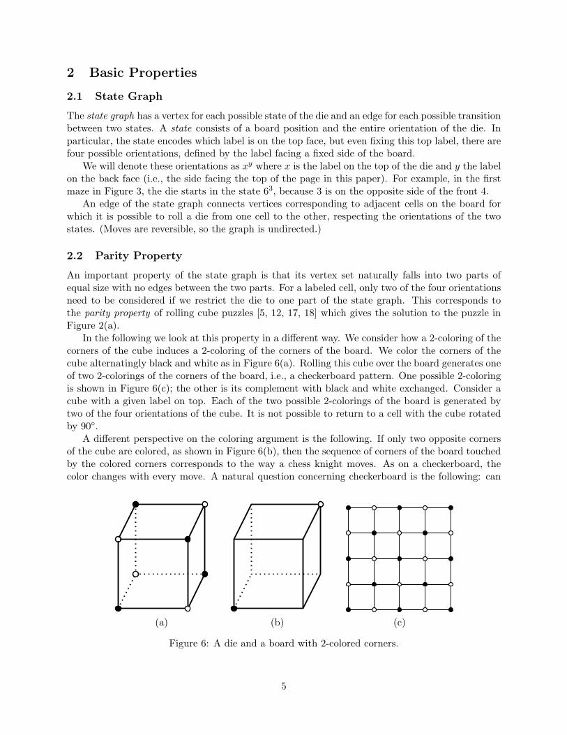
In the following we look at this property in a different way. We consider how a 2-coloring of thecorners of the cube induces a 2-coloring of the corners of the board. We color the corners of thecube alternatingly black and white as in Figure 6(a). Rolling this cube over the board generates oneof two 2-colorings of the corners of the board, i.e., a checkerboard pattern. One possible 2-coloringis shown in Figure 6(c); the other is its complement with black and white exchanged. Consider acube with a given label on top. Each of the two possible 2-colorings of the board is generated bytwo of the four orientations of the cube. It is not possible to return to a cell with the cube rotatedby 90.

A different perspective on the coloring argument is the following. If only two opposite cornersof the cube are colored, as shown in Figure 6(b), then the sequence of corners of the board touchedby the colored corners corresponds to the way a chess knight moves. As on a checkerboard, thecolor changes with every move. A natural question concerning checkerboard is the following: can

(a) (b) (c)

Figure 6: A die and a board with 2-colored corners.

5

5

1 ∗ 6 ∗ 1

1 ∗ 6 ∗ 1

6∗1∗6

6

326

1 1∗1 2 6 5

6 4 ∗ 5 13 65

∗

∗5 4

22

5 3 6 4 2 4

3∗∗

∗ ∗

3∗

Start Goal

2 5

4 ∗∗ 311Orientation

at start

Figure 7: Rolling cube maze using the parity property.

the faces of a cube be colored in black and white in a way that rolling it over a board generates achess board pattern? It is easy to see that this is not the case.

We designed the rolling cube maze in Figure 7 based on an idea of Robert Abbott2 to connectthe two parts of the state graph by a bridge: rolling along the top or bottom row changes the parityof the die. The rules are the same as for the first maze in Figure 3.

2See also http://www.logicmazes.com.

6

2.3 Local Structure

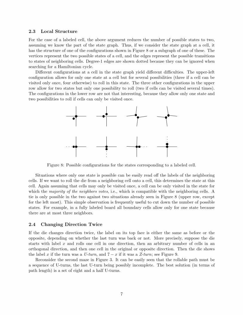
For the case of a labeled cell, the above argument reduces the number of possible states to two,assuming we know the part of the state graph. Thus, if we consider the state graph at a cell, ithas the structure of one of the configurations shown in Figure 8 or a subgraph of one of these. Thevertices represent the two possible states of a cell, and the edges represent the possible transitionsto states of neighboring cells. Degree-1 edges are shown dotted because they can be ignored whensearching for a Hamiltonian cycle.

Different configurations at a cell in the state graph yield different difficulties. The upper-leftconfiguration allows for only one state at a cell but for several possibilities (three if a cell can bevisited only once, four otherwise) to roll in this state. The three other configurations in the upperrow allow for two states but only one possibility to roll (two if cells can be visited several times).The configurations in the lower row are not that interesting, because they allow only one state andtwo possibilities to roll if cells can only be visited once.

Figure 8: Possible configurations for the states corresponding to a labeled cell.

Situations where only one state is possible can be easily read off the labels of the neighboringcells. If we want to roll the die from a neighboring cell onto a cell, this determines the state at thiscell. Again assuming that cells may only be visited once, a cell can be only visited in the state forwhich the majority of the neighbors votes, i.e., which is compatible with the neighboring cells. Atie is only possible in the two against two situations already seen in Figure 8 (upper row, exceptfor the left most). This simple observation is frequently useful to cut down the number of possiblestates. For example, in a fully labeled board all boundary cells allow only for one state becausethere are at most three neighbors.

2.4 Changing Direction Twice

If the die changes direction twice, the label on its top face is either the same as before or theopposite, depending on whether the last turn was back or not. More precisely, suppose the diestarts with label x and rolls one cell in one direction, then an arbitrary number of cells in anorthogonal direction, and then one cell in the original or opposite direction. Then the die showsthe label x if the turn was a U-turn, and 7− x if it was a Z-turn; see Figure 9.

Reconsider the second maze in Figure 3. It can be easily seen that the rollable path must bea sequence of U-turns, the last U-turn being possibly incomplete. The best solution (in terms ofpath length) is a set of eight and a half U-turns.

7

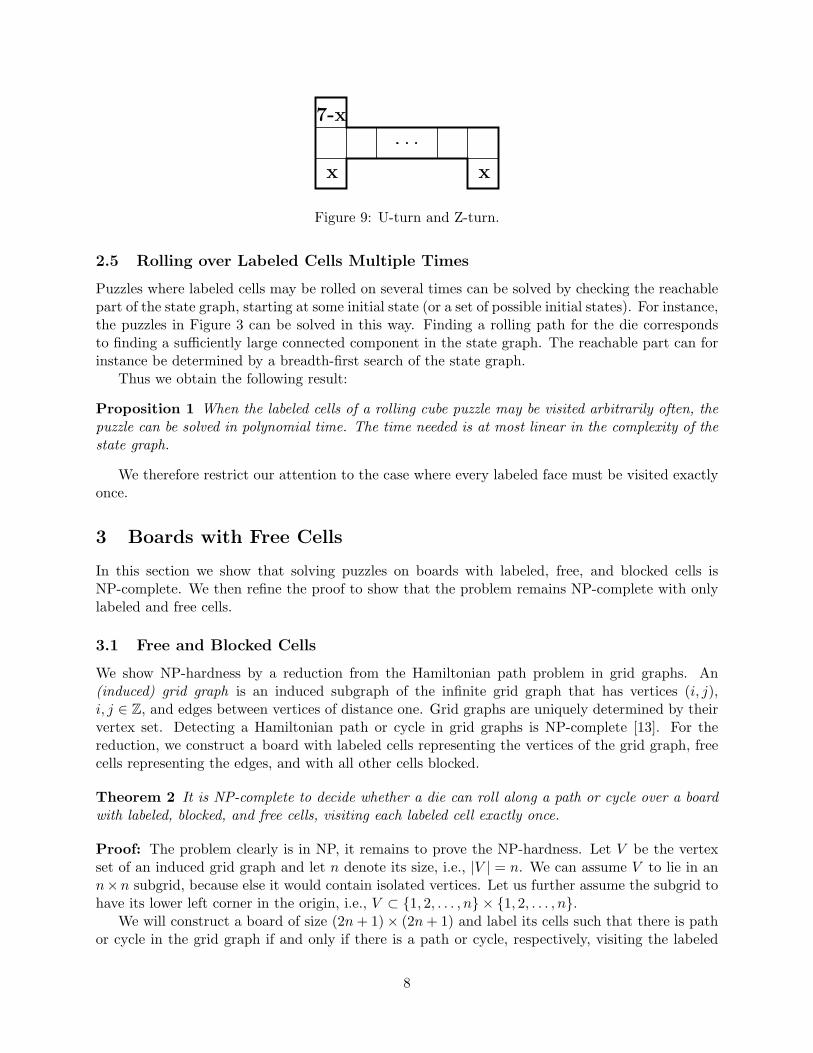
7-x

xx

Figure 9: U-turn and Z-turn.

2.5 Rolling over Labeled Cells Multiple Times

Puzzles where labeled cells may be rolled on several times can be solved by checking the reachablepart of the state graph, starting at some initial state (or a set of possible initial states). For instance,the puzzles in Figure 3 can be solved in this way. Finding a rolling path for the die correspondsto finding a sufficiently large connected component in the state graph. The reachable part can forinstance be determined by a breadth-first search of the state graph.

Thus we obtain the following result:

Proposition 1 When the labeled cells of a rolling cube puzzle may be visited arbitrarily often, thepuzzle can be solved in polynomial time. The time needed is at most linear in the complexity of thestate graph.

We therefore restrict our attention to the case where every labeled face must be visited exactlyonce.

3 Boards with Free Cells

In this section we show that solving puzzles on boards with labeled, free, and blocked cells isNP-complete. We then refine the proof to show that the problem remains NP-complete with onlylabeled and free cells.

3.1 Free and Blocked Cells

We show NP-hardness by a reduction from the Hamiltonian path problem in grid graphs. An(induced) grid graph is an induced subgraph of the infinite grid graph that has vertices (i, j),i, j ∈ Z, and edges between vertices of distance one. Grid graphs are uniquely determined by theirvertex set. Detecting a Hamiltonian path or cycle in grid graphs is NP-complete [13]. For thereduction, we construct a board with labeled cells representing the vertices of the grid graph, freecells representing the edges, and with all other cells blocked.

Theorem 2 It is NP-complete to decide whether a die can roll along a path or cycle over a boardwith labeled, blocked, and free cells, visiting each labeled cell exactly once.

Proof: The problem clearly is in NP, it remains to prove the NP-hardness. Let V be the vertexset of an induced grid graph and let n denote its size, i.e., |V | = n. We can assume V to lie in ann×n subgrid, because else it would contain isolated vertices. Let us further assume the subgrid tohave its lower left corner in the origin, i.e., V ⊂ 1, 2, . . . , n × 1, 2, . . . , n.

We will construct a board of size (2n + 1)× (2n + 1) and label its cells such that there is pathor cycle in the grid graph if and only if there is a path or cycle, respectively, visiting the labeled

8

1

6 1

6 1 6

1

6 1 6

6 1

1

6 1

6 1 6

1

6 1 6

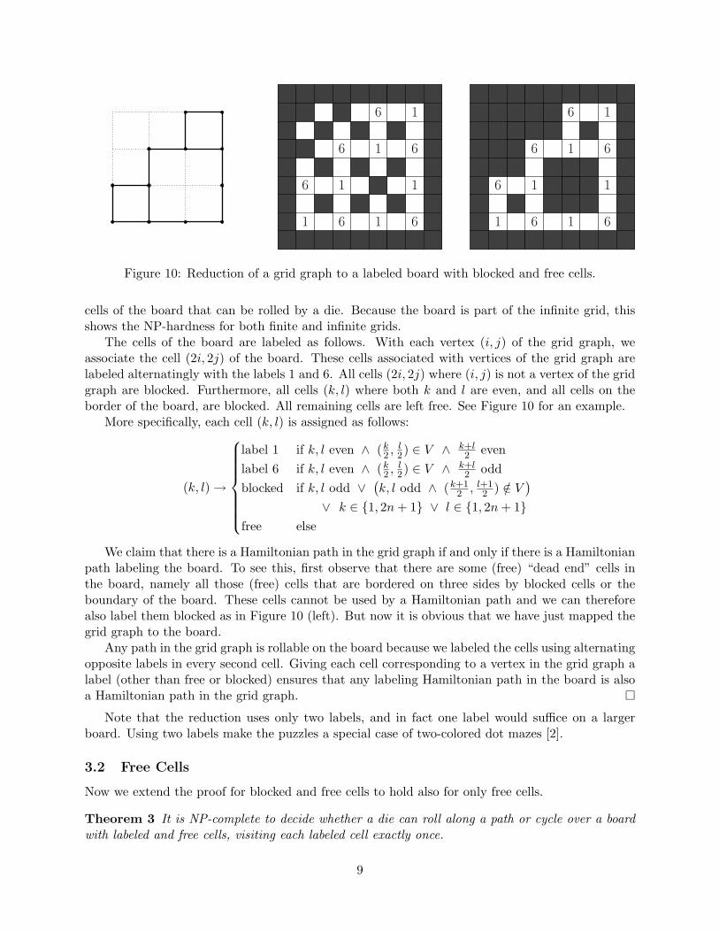
6 1

Figure 10: Reduction of a grid graph to a labeled board with blocked and free cells.

cells of the board that can be rolled by a die. Because the board is part of the infinite grid, thisshows the NP-hardness for both finite and infinite grids.

The cells of the board are labeled as follows. With each vertex (i, j) of the grid graph, weassociate the cell (2i, 2j) of the board. These cells associated with vertices of the grid graph arelabeled alternatingly with the labels 1 and 6. All cells (2i, 2j) where (i, j) is not a vertex of the gridgraph are blocked. Furthermore, all cells (k, l) where both k and l are even, and all cells on theborder of the board, are blocked. All remaining cells are left free. See Figure 10 for an example.

More specifically, each cell (k, l) is assigned as follows:

(k, l) →

label 1 if k, l even ∧ (k2 , l

2) ∈ V ∧ k+l2 even

label 6 if k, l even ∧ (k2 , l

2) ∈ V ∧ k+l2 odd

blocked if k, l odd ∨(k, l odd ∧ (k+1

2 , l+12 ) /∈ V

)∨ k ∈ 1, 2n + 1 ∨ l ∈ 1, 2n + 1

free else

We claim that there is a Hamiltonian path in the grid graph if and only if there is a Hamiltonianpath labeling the board. To see this, first observe that there are some (free) “dead end” cells inthe board, namely all those (free) cells that are bordered on three sides by blocked cells or theboundary of the board. These cells cannot be used by a Hamiltonian path and we can thereforealso label them blocked as in Figure 10 (left). But now it is obvious that we have just mapped thegrid graph to the board.

Any path in the grid graph is rollable on the board because we labeled the cells using alternatingopposite labels in every second cell. Giving each cell corresponding to a vertex in the grid graph alabel (other than free or blocked) ensures that any labeling Hamiltonian path in the board is alsoa Hamiltonian path in the grid graph.

Note that the reduction uses only two labels, and in fact one label would suffice on a largerboard. Using two labels make the puzzles a special case of two-colored dot mazes [2].

3.2 Free Cells

Now we extend the proof for blocked and free cells to hold also for only free cells.

Theorem 3 It is NP-complete to decide whether a die can roll along a path or cycle over a boardwith labeled and free cells, visiting each labeled cell exactly once.

9

1

16 1

6

6

6

66

1 6

6 1

1 6

6 1

1 6

6 1

1 6

6 6

6

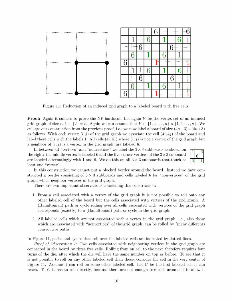
11

Figure 11: Reduction of an induced grid graph to a labeled board with free cells.

Proof: Again it suffices to prove the NP-hardness. Let again V be the vertex set of an inducedgrid graph of size n, i.e., |V | = n. Again we can assume that V ⊂ 1, 2, . . . , n × 1, 2, . . . , n. Weenlarge our construction from the previous proof, i.e., we now label a board of size (4n+3)×(4n+3)as follows. With each vertex (i, j) of the grid graph we associate the cell (4i, 4j) of the board andlabel these cells with the labels 1. All cells (4i, 4j) where (i, j) is not a vertex of the grid graph buta neighbor of (i, j) is a vertex in the grid graph, are labeled 6.

66 1

1 6In between all “vertices” and “nonvertices” we label the 3×3 subboards as shown on

the right: the middle vertex is labeled 6 and the five corner vertices of the 3×3 subboardare labeled alternatingly with 1 and 6. We do this on all 3× 3 subboards that touch atleast one “vertex”.

In this construction we cannot put a blocked border around the board. Instead we have con-structed a border consisting of 3 × 3 subboards and cells labeled 6 for “nonvertices” of the gridgraph which neighbor vertices in the grid graph.

There are two important observations concerning this construction:

1. From a cell associated with a vertex of the grid graph it is not possible to roll onto anyother labeled cell of the board but the cells associated with vertices of the grid graph. A(Hamiltonian) path or cycle rolling over all cells associated with vertices of the grid graphcorresponds (exactly) to a (Hamiltonian) path or cycle in the grid graph.

2. All labeled cells which are not associated with a vertex in the grid graph, i.e., also thosewhich are associated with “nonvertices” of the grid graph, can be rolled by (many different)consecutive paths.

In Figure 11, paths and cycles that roll over the labeled cells are indicated by dotted lines.Proof of Observation 1: Two cells associated with neighboring vertices in the grid graph are

connected in the board by three free cells. Rolling from on cell to the next therefore requires fourturns of the die, after which the die will have the same number on top as before. To see that itis not possible to roll on any other labeled cell than these, consider the cell in the very center ofFigure 11. Assume it can roll on some other labeled cell. Let C be the first labeled cell it canreach. To C it has to roll directly, because there are not enough free cells around it to allow it

10

6

6

6 1

6

6 1

1 6

6 1

6

6

6

1 1

1

66

6

6

61

1

1

6

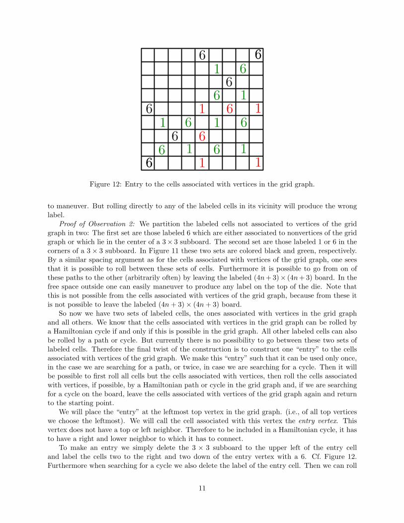
Figure 12: Entry to the cells associated with vertices in the grid graph.

to maneuver. But rolling directly to any of the labeled cells in its vicinity will produce the wronglabel.

Proof of Observation 2: We partition the labeled cells not associated to vertices of the gridgraph in two: The first set are those labeled 6 which are either associated to nonvertices of the gridgraph or which lie in the center of a 3× 3 subboard. The second set are those labeled 1 or 6 in thecorners of a 3× 3 subboard. In Figure 11 these two sets are colored black and green, respectively.By a similar spacing argument as for the cells associated with vertices of the grid graph, one seesthat it is possible to roll between these sets of cells. Furthermore it is possible to go from on ofthese paths to the other (arbitrarily often) by leaving the labeled (4n + 3)× (4n + 3) board. In thefree space outside one can easily maneuver to produce any label on the top of the die. Note thatthis is not possible from the cells associated with vertices of the grid graph, because from these itis not possible to leave the labeled (4n + 3)× (4n + 3) board.

So now we have two sets of labeled cells, the ones associated with vertices in the grid graphand all others. We know that the cells associated with vertices in the grid graph can be rolled bya Hamiltonian cycle if and only if this is possible in the grid graph. All other labeled cells can alsobe rolled by a path or cycle. But currently there is no possibility to go between these two sets oflabeled cells. Therefore the final twist of the construction is to construct one “entry” to the cellsassociated with vertices of the grid graph. We make this “entry” such that it can be used only once,in the case we are searching for a path, or twice, in case we are searching for a cycle. Then it willbe possible to first roll all cells but the cells associated with vertices, then roll the cells associatedwith vertices, if possible, by a Hamiltonian path or cycle in the grid graph and, if we are searchingfor a cycle on the board, leave the cells associated with vertices of the grid graph again and returnto the starting point.

We will place the “entry” at the leftmost top vertex in the grid graph. (i.e., of all top verticeswe choose the leftmost). We will call the cell associated with this vertex the entry vertex. Thisvertex does not have a top or left neighbor. Therefore to be included in a Hamiltonian cycle, it hasto have a right and lower neighbor to which it has to connect.

To make an entry we simply delete the 3 × 3 subboard to the upper left of the entry celland label the cells two to the right and two down of the entry vertex with a 6. Cf. Figure 12.Furthermore when searching for a cycle we also delete the label of the entry cell. Then we can roll

11

onto the (possibly unlabeled) entry vertex from a cell not associated to a vertex in the grid graphby maneuvering in the white space (e.g., from the black 6 on its left, roll two cells yielding a 1 andfrom there two U-turns to the left).

The two cells labeled 6 two cells down and right of the entry vertex, ensure that we roll aHamiltonian cycle on the cells associated with vertices of the grid graph (and not a Hamiltonianpath). Note that, in contrast to the previous proof, we reduce to Hamiltonian cycle and not patheven when searching for a path in the grid, because we can enter the cycle on the grid vertices atany point.

3.3 NP-Hardness and Puzzle Design

We have shown that rolling cube puzzles on boards with free and possibly blocked cells where eachlabeled cell has to be visited exactly once are NP-complete. Does this help us to design difficultpuzzles? It does not immediately help us, because difficult instances of NP-complete problems areusually unsolvable instances. And we are now interested in difficult solvable rolling cube puzzles.In particular, we are not interested in the decision problem but in actually finding a solution.

Similar questions have been asked for the 3-satisfiability (3SAT) problem. Extensive researchhas been done on solving 3SAT instances. To benchmark 3SAT solvers, researchers have consideredempirically difficult instances, in particular difficult positive instances.3 For example, the spin glassapproach [14] creates instances with many local maxima (in the number of satisfied clauses) andonly one satisfying assignment. These are difficult to solve by local search algorithms.

We could construct rolling cube puzzles by starting with a (difficult) 3SAT formula and followingthe reduction. To reduce the size of the resulting puzzle, our reduction can be modified to directlyreduce from planar Hamiltonian cycle [11] or even planar 3SAT [16]. But the resulting puzzles arestill too large.

Empirically difficult 3SAT problems demonstrate that it should be possible to create challengingrolling cube puzzles. However, for us this is still an open problem.

Problem 1 Design a small but difficult rolling cube puzzle (e.g., with many local maxima) wherethe task is to roll over every labeled cell exactly once.

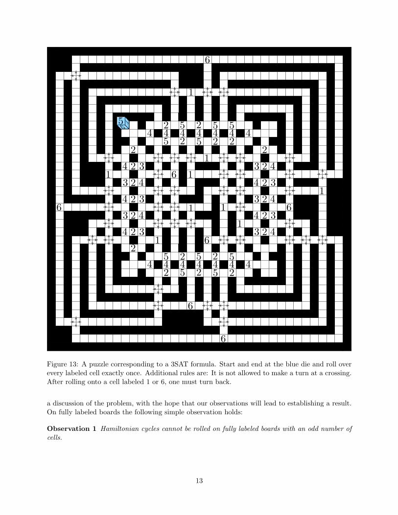
With additional rules it is possible to design smaller puzzles from 3SAT formulas; see Figure 13for an example. The puzzle corresponds to a 3SAT formula with 4 variables (encoded by the sidesof the main square) and 16 clauses (encoded by cells labeled 1 and 6).4 The 3SAT formula is thesmallest nontrivial case of the spin glass approach. The additional rules could be avoided by takinga planar 3SAT instance and by leaving more space between the paths originating from a variablegadget.

4 Boards without Free Cells

What happens when the board contains only labeled and possibly blocked cells? It remains openwhether a polynomial-time algorithm can determine Hamiltonicity of a board, even when all thecells are labeled and when the labeling specifies the orientation of the die. In this section we provide

3A SAT-solver competition is part of the annual International Conference on Theory and Applications of Satisfi-ability Testing.

4The key to the solution is the following. Rolling along the main square in clockwise orientation, the four sides ofthe square are entered by cells labeled 2, 4, 2, and 4. At each of these cells one must choose a direction. The correctdirections are down, left, down, and right.

12

5 46

6

1

2 5 2 5 54444 4 44

122

5 2 5 2 2

2

2

2

2

2

4

4

4

4

4 3

3

3

3

3

6 1

1

1

1 6

1

44

6

1

6

6

6

2

2

2

2

2

4

4

4

4 3

3

3

3

24 31

2 5 2 5 2

5 2 5 2 544444

Figure 13: A puzzle corresponding to a 3SAT formula. Start and end at the blue die and roll overevery labeled cell exactly once. Additional rules are: It is not allowed to make a turn at a crossing.After rolling onto a cell labeled 1 or 6, one must turn back.

a discussion of the problem, with the hope that our observations will lead to establishing a result.On fully labeled boards the following simple observation holds:

Observation 1 Hamiltonian cycles cannot be rolled on fully labeled boards with an odd number ofcells.

13

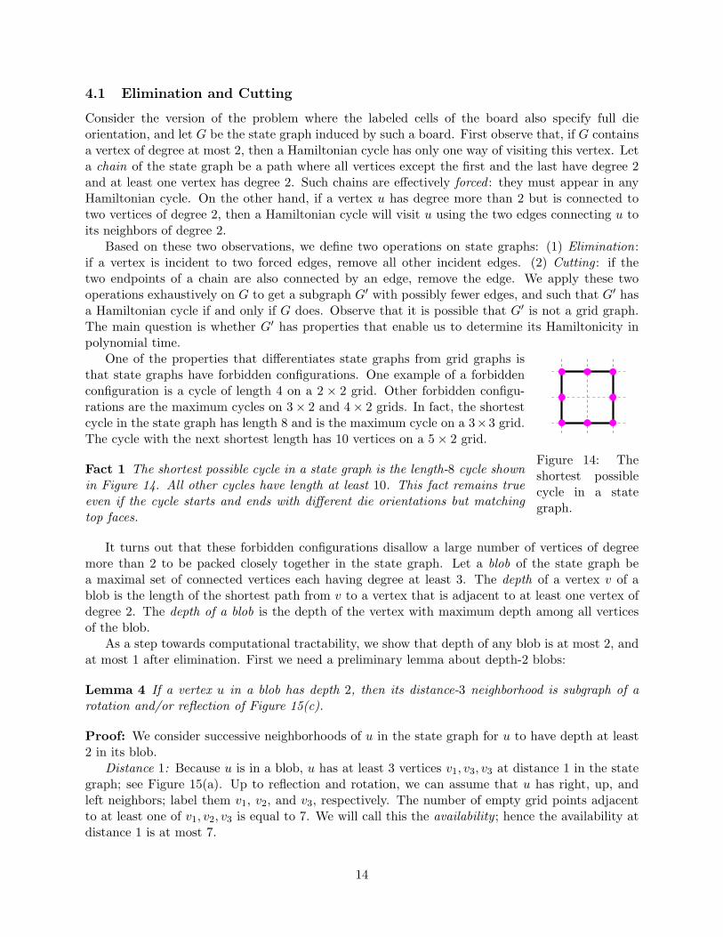
4.1 Elimination and Cutting

Consider the version of the problem where the labeled cells of the board also specify full dieorientation, and let G be the state graph induced by such a board. First observe that, if G containsa vertex of degree at most 2, then a Hamiltonian cycle has only one way of visiting this vertex. Leta chain of the state graph be a path where all vertices except the first and the last have degree 2and at least one vertex has degree 2. Such chains are effectively forced : they must appear in anyHamiltonian cycle. On the other hand, if a vertex u has degree more than 2 but is connected totwo vertices of degree 2, then a Hamiltonian cycle will visit u using the two edges connecting u toits neighbors of degree 2.

Based on these two observations, we define two operations on state graphs: (1) Elimination:if a vertex is incident to two forced edges, remove all other incident edges. (2) Cutting : if thetwo endpoints of a chain are also connected by an edge, remove the edge. We apply these twooperations exhaustively on G to get a subgraph G′ with possibly fewer edges, and such that G′ hasa Hamiltonian cycle if and only if G does. Observe that it is possible that G′ is not a grid graph.The main question is whether G′ has properties that enable us to determine its Hamiltonicity inpolynomial time.

Figure 14: Theshortest possiblecycle in a stategraph.

One of the properties that differentiates state graphs from grid graphs isthat state graphs have forbidden configurations. One example of a forbiddenconfiguration is a cycle of length 4 on a 2 × 2 grid. Other forbidden configu-rations are the maximum cycles on 3× 2 and 4× 2 grids. In fact, the shortestcycle in the state graph has length 8 and is the maximum cycle on a 3×3 grid.The cycle with the next shortest length has 10 vertices on a 5× 2 grid.

Fact 1 The shortest possible cycle in a state graph is the length-8 cycle shownin Figure 14. All other cycles have length at least 10. This fact remains trueeven if the cycle starts and ends with different die orientations but matchingtop faces.

It turns out that these forbidden configurations disallow a large number of vertices of degreemore than 2 to be packed closely together in the state graph. Let a blob of the state graph bea maximal set of connected vertices each having degree at least 3. The depth of a vertex v of ablob is the length of the shortest path from v to a vertex that is adjacent to at least one vertex ofdegree 2. The depth of a blob is the depth of the vertex with maximum depth among all verticesof the blob.

As a step towards computational tractability, we show that depth of any blob is at most 2, andat most 1 after elimination. First we need a preliminary lemma about depth-2 blobs:

Lemma 4 If a vertex u in a blob has depth 2, then its distance-3 neighborhood is subgraph of arotation and/or reflection of Figure 15(c).

Proof: We consider successive neighborhoods of u in the state graph for u to have depth at least2 in its blob.

Distance 1: Because u is in a blob, u has at least 3 vertices v1, v3, v3 at distance 1 in the stategraph; see Figure 15(a). Up to reflection and rotation, we can assume that u has right, up, andleft neighbors; label them v1, v2, and v3, respectively. The number of empty grid points adjacentto at least one of v1, v2, v3 is equal to 7. We will call this the availability ; hence the availability atdistance 1 is at most 7.

14

u

v3 v1

v2

(a) Distance 1 from u in a blob.

w4 w5

v3w3

w2 v2

w1

u

v1 w6

(b) Distance 2 from u of depth at least 1.

w4

v2w2

w1

w5

w3 v3

u

x1

x2

x3

x4

x5

x6

x7 x9

x10

x11

x12

x8

v1 w6

(c) Distance 3 from u of depth at least 2.

Figure 15: The distance-1, -2, and -3 neighborhoods around a vertex u of sufficiently high depthin a blob. Empty squares represent possibly empty grid points within the neighborhood; emptycircles represent possible neighbor locations at the next larger distance.

15

Distance 2: Because u has depth at least 1 in the blob, each of v1, v2, v3 must have degree atleast 3. No vi and vj can have a common neighbor w other than u, because otherwise u, vi, w, vj , uwould be a cycle of length 4, while Fact 1 implies that any cycle in a state graph has length atleast 8. Thus, each of v1, v2, v3 must be adjacent to at least two distinct vertices each adjacent toexactly one of v1, v2, v3. Hence, we need to create at least 3 ·2 = 6 new vertices w1, w2, . . . , w6, eachat distance at most 2 from u in the lattice; see Figure 15(b). Applying an appropriate reflection, v2

has a left neighbor w2. This neighbor forces v3 to have a left and bottom neighbor, while the positionof the remaining vertices w1, w5, w6 remains flexible (provided the grid point above v1 and to theright of v2 is not shared by more than one of v1, v2, v3). Thus we have five different embeddingsof the state graph, modulo rotation and reflection. In all except one of these four embeddings, theavailability is 11, while for the embedding of the graph in Figure 15(b) the availability is 12.

Distance 3: Because u has depth at least 2, each of the 6 vertices w1, w2, . . . , w6 must havedegree at least 3. Again each wi is adjacent to two distinct vertices each adjacent to exactly one wi,because otherwise we would form a cycle of length 6. Thus, we need to create at least 6 · 2 = 12new vertices x1, x2, . . . , x12, each at distance at most 3 from u in the lattice; see Figure 15(c).Thus we need to use the availability-12 embedding of the distance-2 neighborhood state graph inFigure 15(b). Moreover, we claim that the positions of the vertices x1, x2, . . . , x12 are then forced.Vertex w2 can only have a top and left neighbor. As a result, w3 must have a left and bottomneighbor; w4 must have a bottom and right neighbor; w5 must have a bottom and right neighbor;w6 must have a right and top neighbor; and w1 must have a right and top neighbor. Therefore,up to rotation and reflection, Figure 15(c) is the only way of embedding (this subgraph of) thedistance-3 neighborhood on a grid.

Lemma 5 The depth of every blob in a state graph is at most 2.

Proof: Suppose for contradiction that vertex u of a blob has depth greater than 2. By Lemma 4,the distance-3 neighborhood includes as a subgraph the configuration in Figure 15(c) (up to rotationand reflection). Now we proceed to the next level.

Distance 4: Because u has depth at least 3, each of the 12 vertices x1, x2, . . . , x12 must havedegree at least 3. Thus, we need to have at least two new neighbors for each xi. However, thisis impossible. Consider the right neighbor x8 of w4 in Figure 15(c). We cannot give it two moreneighbors without creating a cycle of length less than 8, which contradicts Fact 1. Hence, not allvertices at distance 3 from u have degree at least 3. Therefore, the maximum possible depth of anyvertex in a blob is at most 2.

For the next lemma, we need to avoid degree-1 vertices in the state graph. This condition iscertainly necessary if we wish to find a Hamiltonian cycle. For Hamiltonian paths, there are atmost two such vertices, forcing endpoints of the path, and they can be dealt with separately.

Lemma 6 After applying the elimination operation to every vertex of a state graph having novertices of degree 1, the depth of every blob is at most 1.

Proof: By Lemma 5, the depth of every blob is at most 2. Consider a vertex u of depth 2, andthe required configuration of a subgraph of its distance-3 neighborhood from Lemma 4. If, afterapplying elimination to all the vertices of the graph, vertex u still has depth 2, then every wi stillhas degree at least 3, which in turn implies that at most one of the vertices adjacent to each wi hasdegree 2. Thus, in order for u to have depth 2 after elimination, each wi must be adjacent to atmost one vertex of degree 2. Together with the assumption that we do not have vertices of degree

16

1 in our state graph, we can conclude that we must add at least 18 (= 12 + 6) new edges fromx1, x2, . . . , x12 to the graph.

As in Lemma 5, vertex x8 can have only one new neighbor, on the bottom, because otherwisewe would create a cycle of length less than 8. This neighbor and the degree of x8 forces x7 to havea bottom and left neighbor. Then x6 can have only a left neighbor, so x5 must have a left and topneighbor. Note that, if x7 shared its left neighbor with x6 or a right neighbor with x8, then thiswould create a cycle of length less than 8, contradicting Fact 1. On the other hand, if x4 shared aleft neighbor with x5, this would create a cycle of length 8, but not of the form required by Fact 1,a contradiction. As a result, both x4 and x3 must have degree 2, because no more grid positionsare available to create more neighbors; moreover, they cannot share a neighboring vertex becausethat would create a cycle of length 4. Therefore, w2 has two neighbors of degree 2, causing theelimination operation to disconnect w2 from v2 and thus decreasing u’s depth to at most 1.

Whether the bound on the depth of blobs in state graphs is enough to determine its Hamil-tonicity in polynomial time remains unclear. We conjecture that it is:

Conjecture 1 On boards with labeled and possibly blocked cells, rollable Hamiltonian cycles can bedetermined in polynomial time.

4.2 Uniqueness of Cycles?

At first we conjectured that, if a state graph contains a Hamiltonian cycle, then this cycle is unique.If true, this property would possibly make it easier to determine Hamiltonicity in polynomial time,as it would increase the restrictions on the Hamiltonian cycle if one exists. The conjecture, however,is false for boards that contain blocked cells:

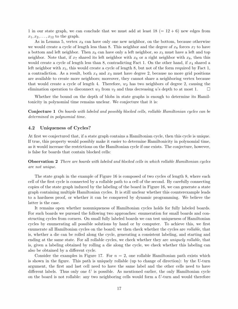
Observation 2 There are boards with labeled and blocked cells in which rollable Hamiltonian cyclesare not unique.

The state graph in the example of Figure 16 is composed of two cycles of length 8, where eachcell of the first cycle is connected by a rollable path to a cell of the second. By carefully connectingcopies of the state graph induced by the labeling of the board in Figure 16, we can generate a stategraph containing multiple Hamiltonian cycles. It is still unclear whether this counterexample leadsto a hardness proof, or whether it can be conquered by dynamic programming. We believe thelatter is the case.

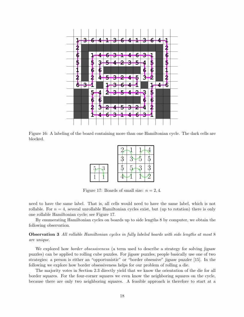
It remains open whether nonuniqueness of Hamiltonian cycles holds for fully labeled boards.For such boards we pursued the following two approaches: enumeration for small boards and con-structing cycles from corners. On small fully labeled boards we can test uniqueness of Hamiltoniancycles by enumerating all possible solutions by hand or by computer. To achieve this, we firstenumerate all Hamiltonian cycles on the board; we then check whether the cycles are rollable, thatis, whether a die can be rolled along the cycle, generating a consistent labeling, and starting andending at the same state. For all rollable cycles, we check whether they are uniquely rollable, thatis, given a labeling obtained by rolling a die along the cycle, we check whether this labeling canalso be obtained by a different cycle.

Consider the examples in Figure 17. For n = 2, one rollable Hamiltonian path exists whichis shown in the figure. This path is uniquely rollable (up to change of direction): by the U-turnargument, the first and last cell need to have the same label and the other cells need to havedifferent labels. Thus only one U is possible. As mentioned earlier, the only Hamiltonian cycleon the board is not rollable: any two neighboring cells would form a U -turn and would therefore

17

1 1 1 1

1

1111

1 1 1

111

33

3

3

5 5

5 4

42

2 2

2

56 4

3

3

2

5

4

4

6452453

6654 6 3 4 6 3

56

62

36436426 63 2 4 5 3 2 4

6

36215623 6 4 3 6 4 3 6 4

265

264

Figure 16: A labeling of the board containing more than one Hamiltonian cycle. The dark cells areblocked.

1

5 3

1

3

5

5

3

1

5

3

12 4

5

32114

Figure 17: Boards of small size: n = 2, 4.

need to have the same label. That is, all cells would need to have the same label, which is notrollable. For n = 4, several unrollable Hamiltonian cycles exist, but (up to rotation) there is onlyone rollable Hamiltonian cycle; see Figure 17.

By enumerating Hamiltonian cycles on boards up to side lengths 8 by computer, we obtain thefollowing observation.

Observation 3 All rollable Hamiltonian cycles in fully labeled boards with side lengths at most 8are unique.

We explored how border obsessiveness (a term used to describe a strategy for solving jigsawpuzzles) can be applied to rolling cube puzzles. For jigsaw puzzles, people basically use one of twostrategies: a person is either an “opportunistic” or “border obsessive” jigsaw puzzler [15]. In thefollowing we explore how border obsessiveness helps for our problem of rolling a die.

The majority votes in Section 2.3 directly yield that we know the orientation of the die for allborder squares. For the four-corner squares we even know the neighboring squares on the cycle,because there are only two neighboring squares. A feasible approach is therefore to start at a

18

corner and to construct the cycle from there, for instance by inductively deducing the edges of thecycle diagonal by diagonal. We show that this is possible at least for the first squares. Let thek-neighborhood of a cell be all cells that can be reached in k steps ignoring the labels of the cells.The following proposition can be proved by a case distinction. It shows that this strategy works atleast to some extent.

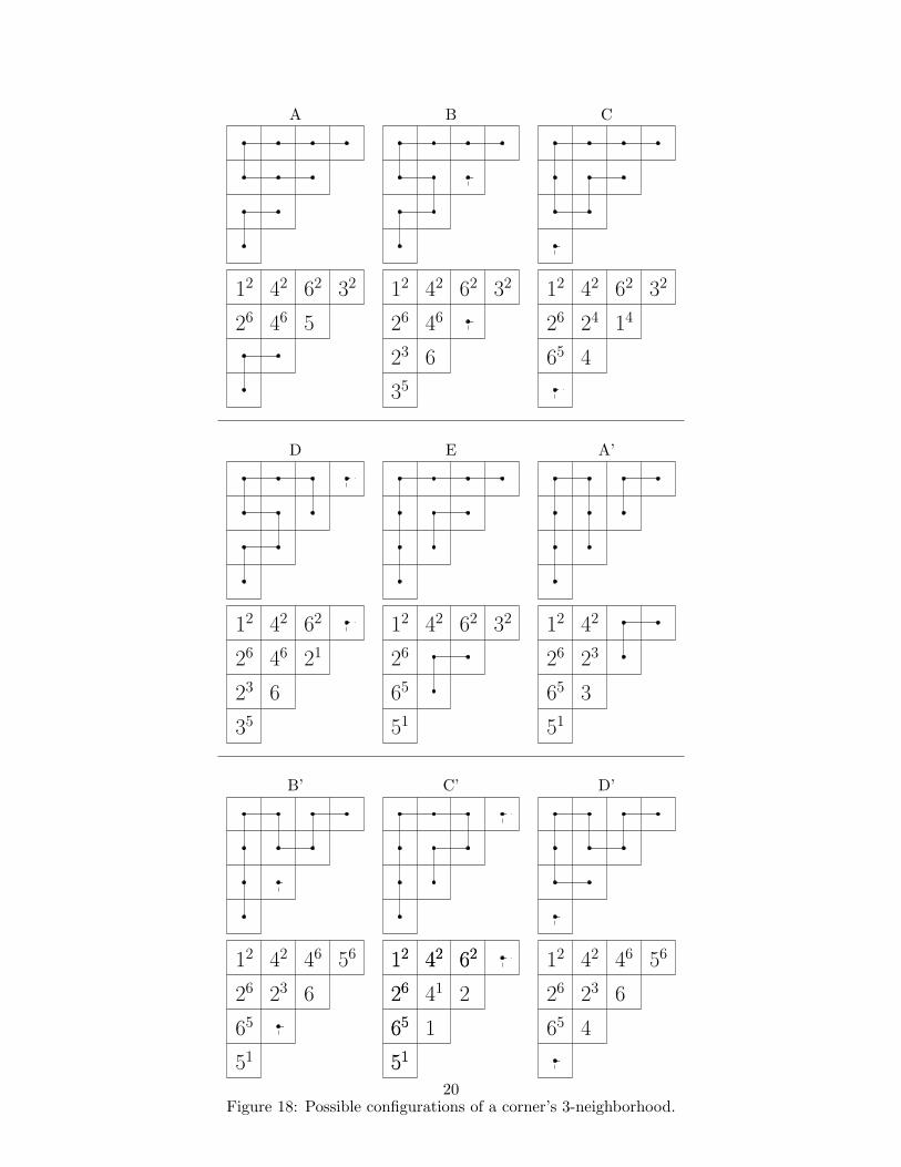
Proposition 7 If a labeling of an n×n board admits a Hamiltonian cycle, then the path of the diewithin the 3-neighborhoods of the corners is unique (up to direction). For n = 4, the rolling patternat a corner is determined by the 2-neighborhood of this corner. For n > 4, the 5-neighborhooddetermines the pattern.

Proof: For n ≤ 3, there is no possibility to roll a cycle. For n = 4, there are two symmetricrollable Hamiltonian cycles, the “H” and the rotated “H”. These two cycles can be distinguishedby looking at a 2-neighborhood of a corner.

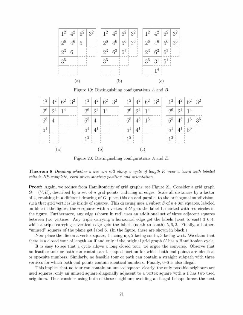
The interesting case is when n > 4. Figure 18 shows all possible 3-neighborhoods of the upper-left corner. For each possibility the rolling pattern is shown and below that the labeling we get ifwe fix the label and orientation of the corner to 12. The cases A′–D′ are symmetric to A–D. Inthe figure we included the orientations of squares which can be deduced using the majority votes(Section 2.3). Assume a set of labels allows for two different rolling patterns in the upper-leftcorner. By overlaying the labelings in Figure 18 we can directly distinguish all cases by looking atthe 3-neighborhood, except possibly the following pairs: (A,B), (A,E), (B,D) and (C,E), and thesymmetric cases (A′, B′), (A′, E), (B′, D′) and (C ′, E). It suffices to consider the first four pairs.

Assume A and B are not distinguishable. Then we are in the situation of Figure 19(a). By amajority vote we actually know that the 5 without orientation is actually a 56. Thus, for B to bepossible the neighbors of this square must be as in Figure 19(b). Now we know that the 6 is a 61

because it cannot connect to its neighboring 62. Also, it must be able to connect to the squarebelow it because the cycle when going through the 6 has only one further possibility. Therefore,the square below is a 31 and to allow B the neighbors of the 31 must be as in Figure 19(b). Nowfinally, it is clear that the 62 must connect to the 56 and to its neighbor below the 36. But thismeans that the 36 cannot connect to this square and therefore must connect to 56. With this weare done because with 62 and 36 connected to 56 it must be pattern B:

The cases A and E are distinguishable because the 46 in case E would require a 63 below it butfor case A the 65 to the left of this square would require a 45 on this square. The cases B and Dcan be handled in the same way: the 32 would require a 24 below it, but the 21 requires a 31 onthe right of it.

The cases C and E are again slightly more involved. The overlay of the labels are shown inFigure 20(a). The 51 needs to connect as shown in Figure 20(b). The 45 needs a 15 to the rightof it as shown in Figure 20(c) and then the neighbors of 15 must be as in Figure 20(d). Then the41 must connect to 51 and below, the 12 must connect to 51 and below. But then we must be incase C.

Thus all patterns are distinguishable, and for this we used at most the 5-neighborhood of acorner.

4.3 Finding Long Rollable Cycles

Suppose we are given a fully labeled board and we ask for a rollable cycle that visits the maximumnumber of cells, without necessarily visiting them all. We show that finding a maximum cycle ona fully labeled board is NP-complete even when we are given a starting position and orientation.

19

A B C

12 42 62 32

26 46 5

12 42 62 32

26 46

623

35

12 42 62 32

26

65 4

24 14

D E A’

12 42 62

26 46

23 6

35

21

12 42 62 32

26

65

51

12 42

26

65

23

51

3

B’ C’ D’

12 42

26

65

23 6

46 56

51

12 42 62

26

65

51

12 42 62

26

65

51

241

1

12 42

26

65

23

4

6

46 56

Figure 18: Possible configurations of a corner’s 3-neighborhood.20

12 42 62 32

26 46

23

35

5

6

12 42 62 32

26 46

23

35

56 36

6263

12 42 62 32

26 46

23

35 31 51

14

56 36

6263

(a) (b) (c)

Figure 19: Distinguishing configurations A and B.

12 42 62 32

26

65

24 14

51

4

12 42 62 32

26

65

24 14

51

4

41

12

12 42 62 32

26

65

24 14

51 41

12

45 15

12 42 62 32

26

65

24 14

51 41

12

45 15

56

35

(a) (b) (c)

Figure 20: Distinguishing configurations A and E.

Theorem 8 Deciding whether a die can roll along a cycle of length K over a board with labeledcells is NP-complete, even given starting position and orientation.

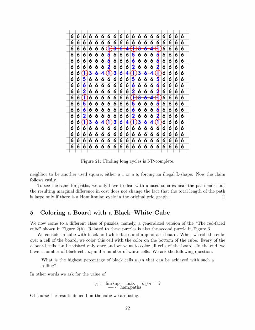
Proof: Again, we reduce from Hamiltonicity of grid graphs; see Figure 21. Consider a grid graphG = (V,E), described by a set of n grid points, inducing m edges. Scale all distances by a factorof 4, resulting in a different drawing of G; place this on and parallel to the orthogonal subdivision,such that grid vertices lie inside of squares. This drawing uses a subset S of n+3m squares, labeledon blue in the figure; the n squares with a vertex of G gets the label 1, marked with red circles inthe figure. Furthermore, any edge (shown in red) uses an additional set of three adjacent squaresbetween two vertices. Any triple carrying a horizontal edge get the labels (west to east) 3, 6, 4,while a triple carrying a vertical edge gets the labels (north to south) 5, 6, 2. Finally, all other,“unused” squares of the plane get label 6. (In the figure, these are shown in black.)

Now place the die on a vertex square, 1 facing up, 2 facing south, 3 facing west. We claim thatthere is a closed tour of length 4n if and only if the original grid graph G has a Hamiltonian cycle.

It is easy to see that a cycle allows a long closed tour; we argue the converse. Observe thatno feasible tour or path can contain an L-shaped portion for which both end points are identicalor opposite numbers. Similarly, no feasible tour or path can contain a straight subpath with threevertices for which both end points contain identical numbers. Finally, 6–6 is also illegal.

This implies that no tour can contain an unused square: clearly, the only possible neighbors areused squares; only an unused square diagonally adjacent to a vertex square with a 1 has two usedneighbors. Thus consider using both of these neighbors; avoiding an illegal I-shape forces the next

21

6

6

6

6

6

6

6

6

6

6

6

6

6

6

6

6

6

6

6

6

6

6

6

6

6

6

6

6

6

6

6

6

6

6

6

6

6

6

6

6

6

6

6

6

6

6

6

6

6

6

6

6

6

6

6

6

6

6

6

6

6

6

6

6

6

6

6

6

6

6

6

6

6

6

6

6

6

6

6

6

6

6

6

6

6

6

6

6

6

6

6

6

6

6

6

6

6

6

6

6

6

6

6

6

6

6

6

6

6

6

6

66

6

6

6

6

6

6

6

6

6

6

6

6

6

6

6

6

6

6

6

6

6

6

6

6

6

6

6

6

6

6

6

6

6

6

6

6

6

6

6

6

6

6

6

6

6

6

6

6

6

6

6

6

6

6

6

6

6

6

6

6

6

6

6

6 6

6 6

6 6

6 6

6 6

6 6

6 6

6 6

6 6

6 66 6

6 6

6 6

6 6

6 6

6 6

6 6

6 6

6 6

6 6

6 6

6 6

6 6

6 6

6 6

6 6

6 6

6 6

6 6

6 6

6 6

6 6

6

6

6

6

6

6

6

6

6

6

6

6

6

6

6

6

6

6

6

6

6

6 6 6 6

6 6

6 66 66 66 6

6 6

6

6

6

6

6

6

6

6 6 6 6 6

6

6

6

6

1 11

1 11

1

1 1 1

1 1

1

6

6

6

6

6

6

6

6

6

6

6

6

6

6 6 6

6

6

2

2

2 2 2

2 2

2 2

55

5

5 5

5

5

5

5

3 3 3

3

3

33

33

4 4 4

4

4

44

44

1

Figure 21: Finding long cycles is NP-complete.

neighbor to be another used square, either a 1 or a 6, forcing an illegal L-shape. Now the claimfollows easily.

To see the same for paths, we only have to deal with unused squares near the path ends; butthe resulting marginal difference in cost does not change the fact that the total length of the pathis large only if there is a Hamiltonian cycle in the original grid graph.

5 Coloring a Board with a Black–White Cube

We now come to a different class of puzzles, namely, a generalized version of the “The red-facedcube” shown in Figure 2(b). Related to these puzzles is also the second puzzle in Figure 3.

We consider a cube with black and white faces and a quadratic board. When we roll the cubeover a cell of the board, we color this cell with the color on the bottom of the cube. Every of then board cells can be visited only once and we want to color all cells of the board. In the end, wehave a number of black cells nb and a number of white cells. We ask the following question:

What is the highest percentage of black cells nb/n that can be achieved with such arolling?

In other words we ask for the value of

qb := lim supn→∞

maxham.paths

nb/n = ?

Of course the results depend on the cube we are using.

22

We will identify all different black-white cubes by the following system. First we count thenumber of black faces fb. If fb is one of 0, 1, 5, 6, then the cube is uniquely described. If fb is 2,we have two variants of the cube: the symmetric variant (two opposite faces are black) and theasymmetric variant (two incident faces are black). For fb = 4, we classify the cube in the same wayby considering the white faces. Finally, if we have three black faces, we call the situation symmetricwhere all of the faces share a vertex and asymmetric otherwise. To distinguish between the differentcube variants, we abbreviate every cube with Cx

fb, where x ∈ ∅, s, a denotes the symmetric or

asymmetric variant if necessary. The problem to find the maximal percentage of black cell is calledthe Cx

fbblackening problem.

In the following, we discuss two cases of the problem in more detail. An interesting case is theCs

3 blackening problem, because it is the perfect equally distributed case and will not give the blackfaces any advantage over the white ones. Another natural question is the C5 blackening problem,which is related to the “red-faced cube” problem introduced by John Harris [6, 8].

5.1 C5 Blackening Problem

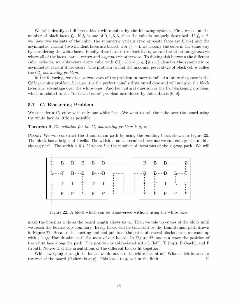
We consider a C5 cube with only one white face. We want to roll the cube over the board usingthe white face as little as possible.

Theorem 9 The solution for the C5 blackening problem is qb = 1.

Proof: We will construct the Hamiltonian path by using the building block shown in Figure 22.The block has a height of 4 cells. The width is not determined because we can enlarge the middlezig-zag path. The width is 6 + 2i where i is the number of iterations of the zig-zag path. We will

L F

B

L T

F F F F F

TT T T T

B B B B B

F

T

B

F

T

BB

FF

TL

L

B

T

B B B B B BB BBB

TL

L

Figure 22: A block which can be transversed without using the white face.

make the block as wide as the board length allows us to. Then we pile up copies of the block untilwe reach the boards top boundary. Every block will be traversed by the Hamiltonian path drawnin Figure 22. Because the starting and end points of the paths of several blocks meet, we come upwith a large Hamiltonian path for most of our board. In Figure 22, one can trace the position ofthe white face along the path. The position is abbreviated with L (left), T (top), B (back), and F(front). Notice that the orientations of the different blocks fit together.

While sweeping through the blocks we do not use the white face at all. What is left is to colorthe rest of the board (if there is any). This leads to qb = 1 in the limit.

23

5.2 Cs3 Blackening Problem

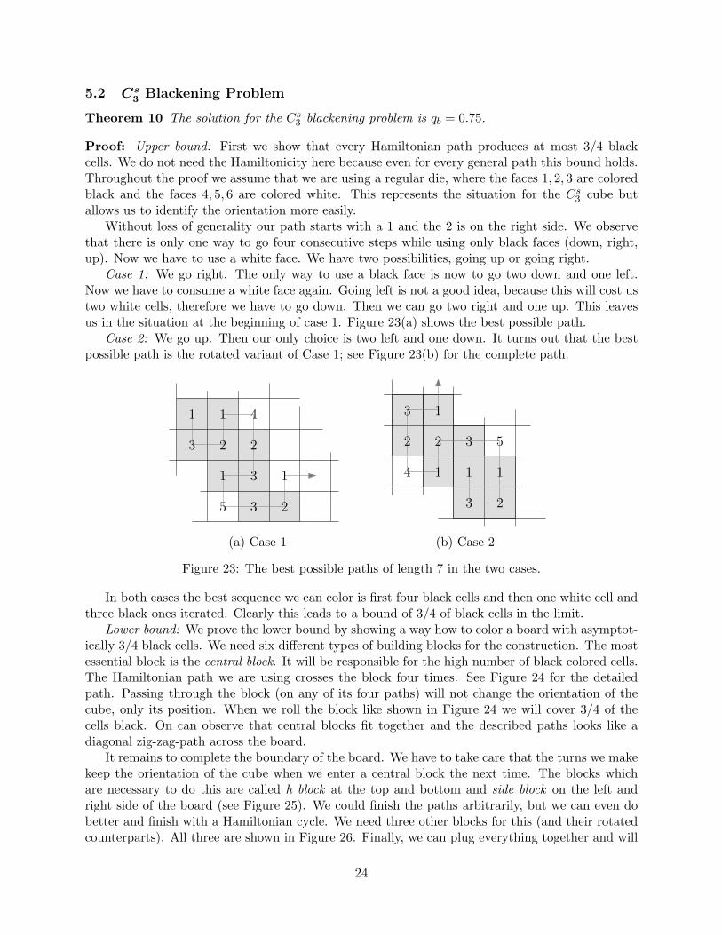
Theorem 10 The solution for the Cs3 blackening problem is qb = 0.75.

Proof: Upper bound: First we show that every Hamiltonian path produces at most 3/4 blackcells. We do not need the Hamiltonicity here because even for every general path this bound holds.Throughout the proof we assume that we are using a regular die, where the faces 1, 2, 3 are coloredblack and the faces 4, 5, 6 are colored white. This represents the situation for the Cs

3 cube butallows us to identify the orientation more easily.

Without loss of generality our path starts with a 1 and the 2 is on the right side. We observethat there is only one way to go four consecutive steps while using only black faces (down, right,up). Now we have to use a white face. We have two possibilities, going up or going right.

Case 1: We go right. The only way to use a black face is now to go two down and one left.Now we have to consume a white face again. Going left is not a good idea, because this will cost ustwo white cells, therefore we have to go down. Then we can go two right and one up. This leavesus in the situation at the beginning of case 1. Figure 23(a) shows the best possible path.

Case 2: We go up. Then our only choice is two left and one down. It turns out that the bestpossible path is the rotated variant of Case 1; see Figure 23(b) for the complete path.

5

4

2

1

2

1

2

3 1

3

1

3

5

4

2

1

2

1

2

3

3

1

3 1

(a) Case 1 (b) Case 2

Figure 23: The best possible paths of length 7 in the two cases.

In both cases the best sequence we can color is first four black cells and then one white cell andthree black ones iterated. Clearly this leads to a bound of 3/4 of black cells in the limit.

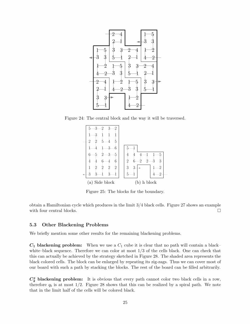
Lower bound: We prove the lower bound by showing a way how to color a board with asymptot-ically 3/4 black cells. We need six different types of building blocks for the construction. The mostessential block is the central block. It will be responsible for the high number of black colored cells.The Hamiltonian path we are using crosses the block four times. See Figure 24 for the detailedpath. Passing through the block (on any of its four paths) will not change the orientation of thecube, only its position. When we roll the block like shown in Figure 24 we will cover 3/4 of thecells black. On can observe that central blocks fit together and the described paths looks like adiagonal zig-zag-path across the board.

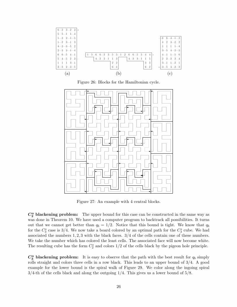
It remains to complete the boundary of the board. We have to take care that the turns we makekeep the orientation of the cube when we enter a central block the next time. The blocks whichare necessary to do this are called h block at the top and bottom and side block on the left andright side of the board (see Figure 25). We could finish the paths arbitrarily, but we can even dobetter and finish with a Hamiltonian cycle. We need three other blocks for this (and their rotatedcounterparts). All three are shown in Figure 26. Finally, we can plug everything together and will

24

2

3 315

2 14

1

1 224

3 35

1

1 224

3 35

1

1 224

3 35

2

3 315

2 14

2

3 315

2 14

2

3 315

2 14

1

1 224

3 35

Figure 24: The central block and the way it will be traversed.

1

5

2

21

1

2

4

2

3 1

6

4

3

1 4

2

3

2

1

3

4

1 1

4

2

3

5

2

3

5

1

5

6

6

3

2

3

6

5

1

4

26 3

2

1

3

514

23

5

1

2

4

3

5

1 4

2

(a) Side block (b) h block

Figure 25: The blocks for the boundary.

obtain a Hamiltonian cycle which produces in the limit 3/4 black cells. Figure 27 shows an examplewith four central blocks.

5.3 Other Blackening Problems

We briefly mention some other results for the remaining blackening problems.

C1 blackening problem: When we use a C1 cube it is clear that no path will contain a black–white–black sequence. Therefore we can color at most 1/3 of the cells black. One can check thatthis can actually be achieved by the strategy sketched in Figure 28. The shaded area represents theblack colored cells. The block can be enlarged by repeating its zig-zags. Thus we can cover most ofour board with such a path by stacking the blocks. The rest of the board can be filled arbitrarily.

Cs2 blackening problem: It is obvious that every path cannot color two black cells in a row,

therefore qb is at most 1/2. Figure 28 shows that this can be realized by a spiral path. We notethat in the limit half of the cells will be colored black.

25

1

5 4

23 2

1

3

5 1

2

6

4

2

3

5

1

2

6

4

6

5

3

1

4

1

3

2

3

1

5

2

3

2 1

3

5

2

4

2

3

5

1

1

5

3

2

1

3

1

1 5 6

4 2

6 3

2 1

3 5

1

2

6 4

2

3

5 1 2 6

4 3

6 5

3 1

5 4

1

3

6 2

3

5

4

1

5

4 2

2

1

1

2

4

2

3

5

1 6

4

6

3

1

4

1

3

2

1

3

2

1 4

3

4

3

1

1

3 4

6

2

3

5

2

3

(a) (b) (c)

Figure 26: Blocks for the Hamiltonian cycle.

Figure 27: An example with 4 central blocks.

Ca2 blackening problem: The upper bound for this case can be constructed in the same way as

was done in Theorem 10. We have used a computer program to backtrack all possibilities. It turnsout that we cannot get better than qb = 1/2. Notice that this bound is tight. We know that qb

for the Cs3 case is 3/4. We now take a board colored by an optimal path for the Cs

3 cube. We hadassociated the numbers 1, 2, 3 with the black faces. 3/4 of the cells contain one of these numbers.We take the number which has colored the least cells. The associated face will now become white.The resulting cube has the form Cs

2 and colors 1/2 of the cells black by the pigeon hole principle.

Ca3 blackening problem: It is easy to observe that the path with the best result for qb simply

rolls straight and colors three cells in a row black. This leads to an upper bound of 3/4. A goodexample for the lower bound is the spiral walk of Figure 29. We color along the ingoing spiral3/4-th of the cells black and along the outgoing 1/4. This gives us a lower bound of 5/8.

26

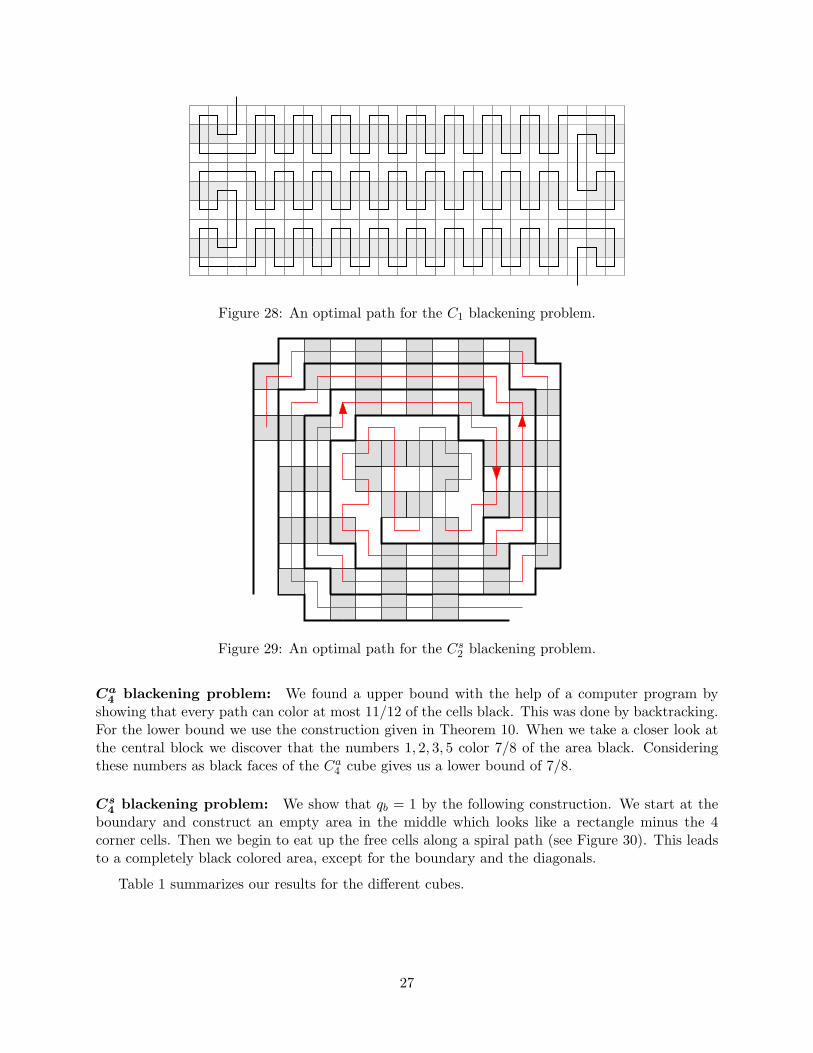
Figure 28: An optimal path for the C1 blackening problem.

Figure 29: An optimal path for the Cs2 blackening problem.

Ca4 blackening problem: We found a upper bound with the help of a computer program by

showing that every path can color at most 11/12 of the cells black. This was done by backtracking.For the lower bound we use the construction given in Theorem 10. When we take a closer look atthe central block we discover that the numbers 1, 2, 3, 5 color 7/8 of the area black. Consideringthese numbers as black faces of the Ca

4 cube gives us a lower bound of 7/8.

Cs4 blackening problem: We show that qb = 1 by the following construction. We start at the

boundary and construct an empty area in the middle which looks like a rectangle minus the 4corner cells. Then we begin to eat up the free cells along a spiral path (see Figure 30). This leadsto a completely black colored area, except for the boundary and the diagonals.

Table 1 summarizes our results for the different cubes.

27

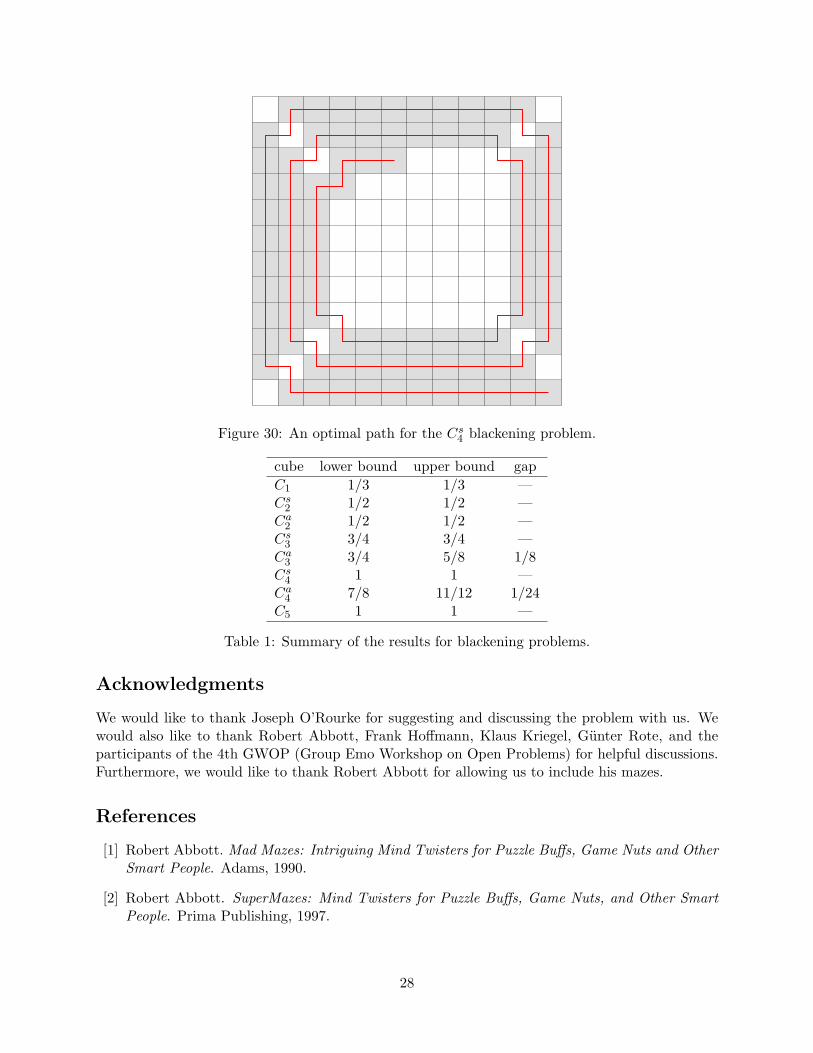
Figure 30: An optimal path for the Cs4 blackening problem.

cube lower bound upper bound gapC1 1/3 1/3 —Cs

2 1/2 1/2 —Ca

2 1/2 1/2 —Cs

3 3/4 3/4 —Ca

3 3/4 5/8 1/8Cs

4 1 1 —Ca

4 7/8 11/12 1/24C5 1 1 —

Table 1: Summary of the results for blackening problems.

Acknowledgments

We would like to thank Joseph O’Rourke for suggesting and discussing the problem with us. Wewould also like to thank Robert Abbott, Frank Hoffmann, Klaus Kriegel, Gunter Rote, and theparticipants of the 4th GWOP (Group Emo Workshop on Open Problems) for helpful discussions.Furthermore, we would like to thank Robert Abbott for allowing us to include his mazes.

References

[1] Robert Abbott. Mad Mazes: Intriguing Mind Twisters for Puzzle Buffs, Game Nuts and OtherSmart People. Adams, 1990.

[2] Robert Abbott. SuperMazes: Mind Twisters for Puzzle Buffs, Game Nuts, and Other SmartPeople. Prima Publishing, 1997.

28

[3] Robert Abbott. A maze with rules. In Martin Gardner, Elwyn Berlekamp, and Tom Rodgers,editors, The Mathemagician and Pied Puzzler: A Collection in Tribute to Martin Gardner,pages 27–28. AK Peters, Ltd, 1999.

[4] Erik D. Demaine and Joseph O’Rourke. Open problems from CCCG 2005. In Proc. 18thCanadian Conference on Computational Geometry (CCCG’06), pages 75–80, 2006.

[5] Martin Gardner. Mathematical games column. Scientific American, 209(6):144, December1963. Solution in January 1964 column.

[6] Martin Gardner. Mathematical games column. Scientific American, 213(5):120–123, November1965. Problem 9. Solution in December 1965 column.

[7] Martin Gardner. Martin Gardner’s Sixth Book of Mathematical Diversions from ScientificAmerican. W H Freeman, San Francisco, 1971. Chapter 8.

[8] Martin Gardner. Mathematical Carnival. Borzoi / Alfred A Knopf, New York, 1975. Chapter9, Problem 1: The red-faced cube.

[9] Martin Gardner. Mathematical games column. Scientific American, 232(3):112–116, March1975. Solution in April 1975 column.

[10] Martin Gardner. Time Travel and Other Mathematical Bewilderments. W H Freeman, NewYork, 1988. Chapter 9, Problem 8: Rolling cubes.

[11] M. R. Garey, D. S. Johnson, and R. Endre Tarjan. The planar Hamiltonian circuit problem isNP-complete. SIAM Journal on Computing, 5(4):704–714, 1976.

[12] John Harris. Single vacancy rolling cube problems. J. Recreational Mathematics, 7(3):220–223,1974.

[13] Alon Itai, Christos H. Papadimitriou, and Jayme Luiz Szwarcfiter. Hamilton paths in gridgraphs. SIAM J. Comput., 11(4):676–686, 1982.

[14] Haixia Jia, Cristopher Moore, and Bart Selman. From spin glasses to hard satisfiable formulas.In Theory and Applications of Satisfiability Testing, 7th Intl. Conf. (SAT 2004), volume 3542of Lecture Notes in Computer Science, pages 199–210. Springer, 2005.

[15] Hilary Johnson and Joanne Hyde. Towards modeling individual and collaborative construc-tion of jigsaws using task knowledge structures (tks). ACM Trans. Comput.-Hum. Interact.,10(4):339–387, 2003.

[16] David Lichtenstein. Planar formulae and their uses. SIAM Journal on Computing, 11(2):329–343, 1982.

[17] Ronald Sprague. Unterhaltsame Mathematik. Vieweg & Sohn, Braunschweig, 1961. Problem3: Schwere Kisten.

[18] Ronald Sprague. Recreations in Mathematics. Blackie, Glasgow, 1963. Problem 3: HeavyBoxes. Translation by T. H. O’Beirne.

[19] Charles W. Trigg. Tetrahedron rolled onto a plane. J. Recreational Mathematics, 3(2):82–87,1970.

29

[20] M. Oskar van Deventer. Rolling block mazes. In Barry Cipra, Erik D. Demaine, Martin L.Demaine, and Tom Rodgers, editors, Tribute to a Mathemagician, pages 241–250. AK Peters,Ltd, 2004.

30