On One-Dimensional Stretching - NASA · On One-Dimensional Stretching ... with elliptical cross...
56
NASA Contractor Report 3313 On One-Dimensional Stretching Functions for Finite- Difference Calculations Marcel Vinokur University of Samtu Clara Saizta Clara, Califoriiia Prepared for Ames Research Center under Grant NSG-2086 National Aeronautics and Space Administration Scientific and Technical Information Branch 1980 https://ntrs.nasa.gov/search.jsp?R=19800025680 2018-07-22T10:03:53+00:00Z
Transcript of On One-Dimensional Stretching - NASA · On One-Dimensional Stretching ... with elliptical cross...

NASA Contractor Report 3313
On One-Dimensional Stretching Functions for Finite- Difference Calculations
Marcel Vinokur University of Samtu Clara Saizta Clara, Califoriiia
Prepared for Ames Research Center under Grant NSG-2086
National Aeronautics and Space Administration
Scientific and Technical Information Branch
1980
https://ntrs.nasa.gov/search.jsp?R=19800025680 2018-07-22T10:03:53+00:00Z

INDEX
i
ii
I. INTRODUCTION
I I. TRUNCATION ERROR ANALYSIS FOR ONE-DIMENSIONAL STRETCHING
FUNCTIONS
111. A GENERAL TWO-SIDED STRETCHING FUNCTION
I V .
V . CONCLUDING REMARKS V I . REFERENCES
A GENERAL INTERIOR STRETCHING FUNCTION
APPENDIX A: EVALUATION OF ANTI-SYMMETRIC TWO-SIDED STRETCHING
FUNCTIONS
INVERSION OF y = s inh x / x INVERSION OF y = sin x /x
FUNCTION DERIVED FROM w = t anz
APPENDIX B: APPENDIX C:
APPENDIX D: SOLUTION CHARACTERISTICS OF THE TWO-SIDED STRETCHING
APPENDIX E: EVALUATION OF ANTI-SYMMETRIC INTERIOR STRETCHING
FUNCTIONS
1 4
9
18 22
27
28
34 38
40
48

Figure 1. Two-sided Stretching Function f o r So = 100 26
Figure D. 1. Solution Characterist ics of Two-sided Stretching 46 and Different Values of S1
Functions Derived from w = tanz Figure D.2. Locus of Solution i n z-Plane 47
i

ABSTRACT
The class of one-dimens difference calculations
onal stretching functions used in f i n i s studied. For solutions containing
te- a highly
localized region of rapid variation, simple c r i t e r i a for a stretching function are derived using a truncation e r ror analysis. These c r i t e r i a are used t o investigate two types of stretching functions. One i s an i n t e r io r stretching function, fo r which the location and slope of an i n t e r io r clustering region are specified. The simplest such function sat isfying the c r i t e r i a i s found t o be one based on the inverse hyperbolic sine. type of function i s a two-sided stretching function, for which the a rb i t ra ry slopes a t the two ends of the one-dimensional interval are specified. The simplestsuch general function is found t o be one based on the inverse tangent. b o t h equal and greater than one was f i r s t employed by Roberts. general two-sided function has many applications in the construction Of
f ini te-difference grids. of the references.
I t was f i r s t employed by Thomas e t a l . The other
The special case where the slopes were The
An example o f such an application i s found in one
ii

I . INTRODUCTION
F i n i t e - d i f f e r e n c e c a l c u l a t i o n s o f f l u i d f l o w problems a r e bes t c a r r i e d
o u t u s i n g an equispaced g r i d i n a r e c t a n g u l a r ( o r c u b i c ) computat ional
domain, w i t h t h e f l o w v a r i a b l e s and components o f t h e p o s i t i o n v e c t o r
as dependent v a r i a b l e s , and boundary c o n d i t i o n s a p p l i e d a t t h e edges
( o r f aces ) o f t h e domain. I n o r d e r t o min imize t h e number o f g r i d p o i n t s r e q u i r e d f o r a g i ven accuracy, one seeks b o u n d a r y - f i t t e d coo rd ina te t rans fo rma t ions t h a t c l u s t e r p o i n t s i n reg ions where t h e dependent
v a r i a b l e s undergo r a p i d v a r i a t i o n .
geometry ( v e r y l a r g e cu rva tu res o r co rne rs ) , c o m p r e s s i b i l i t y (en t ropy
l a y e r s , shock waves and c o n t a c t d i s c o n t i n u i t i e s ) , and v i s c o s i t y (boundary
l a y e r s and shear l a y e r s ) .
o f such reg ions o f va r ious l e n g t h scales, and o f t e n o f unknown l o c a t i o n .
An i d e a l g r i d would a d j u s t w i t h each t ime o r i t e r a t i o n s tep t o m a i n t a i n optimum c l u s t e r i n g . Such adap t i ve g r i d methods, which i n v o l v e t h e
s o l u t i o n o f a u x i l i a r y equat ions, have been developed f o r one-dimensional
problems ( r e f s . 1 -3 ) . T h e i r ex tens ion t o complex mu l t i - d imens iona l
f l o w s i s a d i f f i c u l t problem, p a r t i c u l a r l y when t h e r e g i o n s r e q u i r i n g
c l u s t e r i n g do n o t have s imple t o p o l o g i c a l p r o p e r t i e s r e q u i r e d by a f i n i t e - d i f f e r e n c e g r i d .
These r e g i o n s may be due t o body
A complex f l o w may thus c o n t a i n a v a r i e t y
There a r e many p r a c t i c a l problems i n which t h e l o c a t i o n s and l e n g t h scales of r e g i o n s o f r a p i d v a r i a t i o n can be est imated a p r i o r i
(e.g., known geometry, a t tached boundary l a y e r s , s imple shock wave c o n f i g u r a t i o n s ) . I n these cases t h e c l u s t e r i n g can be i nco rpo ra ted
i n automat ic g r i d generators which so l ve an e l l i p t i c boundary-value
problem ( r e f s . 4-6) . The d i s t r i b u t i o n o f g r i d p o i n t s on t h e boundaries i s then no rma l l y p resc r ibed a l g e b r a i c a l l y , u s i n g one-dimensional
s t r e t c h i n g f u n c t i o n s . (Here, s t r e t c h i n g f u n c t i o n r e f e r s t o any
t r a n s f o r m a t i o n i n v o l v i n g s t r e t c h i n g o r c l u s t e r i n g ) .
t o employ s t r e t c h i n g f u n c t i o n s t o o b t a i n a c l u s t e r e d g r i d f rom an
unc lus te red g r i d by app ly ing c l u s t e r i n g t o one coo rd ina te f a m i l y o n l y .
For some simple geometries, one can c o n s t r u c t e n t i r e c l u s t e r e d g r i d s
p u r e l y a l g e b r a i c a l l y , u s i n g o n l y one-dimensional s t r e t c h i n g f u n c t i o n s .
It i s a l s o p o s s i b l e
1

The s imp les t c l a s s o f one-dimensional s t r e t c h i n g f u n c t i o n s i s t h a t
i n v o l v i n g two parameters. I n i n t e r i o r s t r e t c h i n g f u n c t i o n s , t h e
parameters a r e t h e l o c a t i o n and s lope o f a s i n g l e c l u s t e r i n g reg ion .
I n two-sided s t r e t c h i n g f u n c t i o n s , t h e s lopes a t t h e two ends o f t h e one -d imens i onal i n t e r v a l a r e s pec i f i ed . .The a n t i - symmetri c two - s i ded
s t r e t c h i n g f u n c t i o n ( w i t h t h e same s lope a t each end) i s o f spec ia l
i n t e r e s t , s ince t h e p o r t i o n f rom t h e m i d p o i n t t o e i t h e r end d e f i n e s
a one-sided s t r e t c h i n g func t i on ( w i t h zero cu rva tu re a t t h e o t h e r
end).
case o f t h e i n t e r i o r s t r e t c h i n g f u n c t i o n , by l o c a t i n g the c l u s t e r i n g r e g i o n a t one end.
case, these two one-sided s t r e t c h i n g f u n c t i o n s a r e o f a d i f f e r e n t nature.
A one-sided s t r e t c h i n g f u n c t i o n can a l s o be obta ined as a spec ia l
Since the c l u s t e r e d end has zero cu rva tu re i n t h i s
An i n t e r i o r s t r e t c h i n g f u n c t i o n based on t h e i nve rse h y p e r b o l i c s i n e was
employed by Thomas, Vinokur, Bast ianon, and Cont i ( r e f . 7 ) i n a
numerical s o l u t i o n of i n v i s c i d supersonic f l o w over a b l u n t d e l t a wing w i t h e l l i p t i c a l c ross sec t i on . The f u n c t i o n was used t o c l u s t e r p o i n t s
on t h e body a t t h e v e r t i c e s o f ve ry e c c e n t r i c e l l i p s e s . The one-sided
v e r s i o n c l u s t e r e d p o i n t s i n t h e f l o w near t h e body su r face t o r e s o l v e
t h e en t ropy l a y e r due t o t h e bow shock. No d e r i v a t i o n of t h e s t r e t c h i n g
f u n c t i o n was given, and t h e c l u s t e r i n g parameter appear ing i n i t was n o t
r e l a t e d t o t h e l e n g t h scales o f reg ions o f r a p i d v a r i a t i o n i n p h y s i c a l
space.
An ant i -symmetr ic two-sided s t r e t c h i n g f u n c t i o n o f a l o g a r i t h m i c t y p e
was employed by Roberts ( r e f . 8) t o s tudy boundary l a y e r f l ows .
h e u r i s t i c d e r i v a t i o n o f t h e f u n c t i o n avoided c o n s i d e r a t i o n o f t h e
t r u n c a t i o n e r r o r s assoc ia ted w i t h f i n i t e - d i f f e r e n c e approx imat ions.
Whi le t h i s f u n c t i o n has been used success fu l l y i n many f l o w c a l c u l a t i o n s ,
t h e r e i s a need f o r a genera l two-sided f u n c t i o n which a l l o w s a r b i t r a r y
s t r e t c h i n g o r c l u s t e r i n g t o be s p e c i f i e d independent ly a t each end. An
a p p l i c a t i o n would be problems i n which t h e a p p r o p r i a t e l e n g t h scales
r e q u i r i n g c l u s t e r i n g a r e s i g n i f i c a n t l y d i f f e r e n t a t t he two ends.
a p p l i c a t i o n i s t h e d i s t r i b u t i o n o f g r i d p o i n t s on a curve which i s
The
Another
2

d e f i n e d piecewise, where c o n t i n u i t y o f g r i d spacing i s d e s i r e d a t t h e
ends o f t h e p iecewise segments.
a f u n c t i o n as a b lending o r i n t e r p o l a t i n g f u n c t i o n t o c o n s t r u c t two
and three-dimensional g r i d s u s i n g one-dimensional s t r e t c h i n g f u n c t i o n s
and shear ing t rans fo rma t ion .
ordered g r i d f o r wing body f l o w s by Yinokur ( r e f . 9) i s an example o f
these a p p l i c a t i o n s .
A t h i r d a p p l i c a t i o n i s t h e use o f such
The c o n s t r u c t i o n o f a s i n g l e , w e l l -
The p resen t work has two o b j e c t i v e s .
c r i t e r i a f o r one-dimensional s t r e t c h i n g f u n c t i o n s , by cons ide r ing t h e
t r u n c a t i o n e r r o r s i n h e r e n t i n f i n i t e - d i f f e r e n c e approximat ions. The
f u n c t i o n s i n t roduced by Thomas e t a1 and Roberts w i l l be found t o be
t h e s i m p l e s t ones s a t i s f y i n g these c r i t e r i a .
d e r i v e a s imple form of t h e genera l two-sided s t r e t c h i n g f u n c t i o n .
One i s t o o b t a i n s imple, r a t i o n a l
The o t h e r o b j e c t i v e i s t o
3

11. TRUNCATION ERROR ANALYSIS FOR ONE-DIMENSIONAL STRETCHING FUNCTIONS
An exac t a n a l y s i s of t h e t r u n c a t i o n e r r o r i nhe ren t i n a f i n i t e - d i f f e r e n c e
c a l c u l a t i o n would r e q u i r e knowledge o f t h e equat ion being so lved and t h e
f i n i t e d i f f e rence approx imat ion t h a t i s used. Here we a r e concerned w i t h t h e spec ia l s i t u a t i o n where t h e s o l u t i o n con ta ins a h i g h l y l o c a l i z e d
r e g i o n of r a p i d v a r i a t i o n w i t h respec t t o some coord inate, and we seek
approximate c r i t e r i a f o r a s t r e t c h i n g f u n c t i o n t h a t w i l l be independent
o f t h e equat ion o r d i f f e r e n c e a lgo r i t hm. approximated a r e i n general n o n - l i n e a r f u n c t i o n s o f t he unknowns and
t h e i r s p a t i a l d e r i v a t i v e s . The e r r o r a n a l y s i s w i l l be performed i n
terms o f t h e f r a c t i o n a l t r u n c a t i o n e r r o r s f o r t h e s p a t i a l d e r i v a t i v e s .
The q u a n t i t i e s t h a t a r e
L e t F(t) be t h e equat ion d e s c r i b i n g a 5 -coo rd ina te curve, where t i s
any parameter t h a t v a r i e s smoothly w i t h a r c l eng th .
t h e ends o f t h e curve, we i n t r o d u c e t h e normal ized v a r i a b l e s
I f A and B denote
rang ing f rom 0 t o 1. For s i m p l i c i t y , a l l p a r t i a l d e r i v a t i v e s w i t h
respec t t o 5 o r t w i l l be w r i t t e n as t o t a l d e r i v a t i v e s . L e t @ ( t ) be
any f u n c t i o n o f t h e unknowns. Outside o f t h e r e g i o n where
we can d e f i n e a n a t u r a l l e n g t h s c a l e o f t h e v a r i a t i o n o f $I
t o t as
d$I/dt = 0,
w i t h respec t
Since t h e components o f
c a l c u l a t i o n o f m e t r i c s and Jacobians, we s i m i l a r l y d e f i n e t h e n a t u r a l
l e n g t h s c a l e o f t h e v a r i a t i o n o f
a l s o e n t e r as dependent v a r i a b l e s i n t h e
w i t h respec t t o t as
4

Note t h a t i f t i s p r o p o r t i o n a l t o a rc l eng th , then Lrt i s p r e c i s e l y
t h e r a d i u s of curva ture , normal ized by t h e l e n g t h o f t h e curve,
Assume f i r s t t h a t t i s used as the normal ized computat ional v a r i a b l e
( i . e . 5 = t ) , w i t h A t as t h e u n i f o r m g r i d spacing.
f i n i t e d i f fe rence approx imat ion t o d$ /d t .
w r i t e any f i r s t o rde r accura te approx imat ion as
L e t 6@/6 t denote t h e
Using equat ion ( 2 ) , one can
6 % = + $ + o
S i m i l a r y, t h e approximat on t o dF/dt can be w r i t t e n as
-+ - sF= x[ l d r t 0 A t ) ] . 6 t
I f L-’Ot o r L- rt became ve ry l a r g e i n some l o c a l i z e d reg ion , then a
p r o h i b i t i v e l y small A t would be r e q u i r e d t o o b t a i n a des i red f r a c t i o n a l
t r u n c a t i o n e r r o r .
o f g r i d p o i n t s would be wasted.
and L-’ $ E r S computat ional v a r i a b l e E; f o r which L-
cou ld be l o c a l y very l a r g e . though L - l +t o r L - l r t
Outs ide o f t he l o c a l i z e d reg ion , t he excess ive number
The obvious remedy i s t o seek a new
remain o f 0 (1) , even
Wi th the a i d o f t h e i d e n t i t i e s
and ,-.
and d e f i n i t i o n (2 ) , one can e a s i l y show t h a t

Similarly, using definition (3) , one obtains the inequality
One criterion for the stretching function C(t) is therefore
In addition, we require that
and d t 1 - L- rt dg = O(1).
Consider the case where L-l follows from equation (11) that
is very large in some localized region. It 9t
in that region. Since L-l thickness is of O(L interval. Furthermore, since L-l region, it follows from equation (11) that dt/dC = 0(1), i.e. that dt/dC does not become large anywhere. are satisfied if condition (10) i s valid.
remains large over an interval whose v- ) , we require that dt/d< remains small over that @t
= 0(1) outside of the localized @t
But these two additional requirements Noting that
it follows upon integration over a finite interval At that
6

Applying equation (15) to the localized region, for which At = O(L
we find,using equation (lo), that ) , $t
Thus equation (13) is satisfied over the entire localized region. Gt = 1 in equation (15), we see that dt/dE = 0(1) is satisfied over the complete range of t. In the event tnat L-lrt is larger than L-l +t in the localized region, then condition (13) is replaced by
Letting
The above analysis is easily extended to higher order finite-difference approximations, as well as the treatment o f higher derivatives. to consider fractional truncation errors due to a second-order accurate approximation to d$/dt (and also for regions where d $/dt2 = 0), it is appropriate to define a different length scale of the variation of$with respect to t as
In order
2
We now require that L-’ remains of 0(1), even though r-’ very large. Using the identity
could be locally $ E $t
we obtain the inequality
;-2 5 - 1 dt)2 dt -2 +E - (L- @t dg
In addition to satisfy must sat i sfy
- = O ( tc
ng equation (lo), the stretching function t;(t)
1. (21 1
7

i n t h e l o c a l i z e d reg ion , c o n d i t i o n (13) @t
Also, i f L-' must be rep laced by
i s l a r g e r t h a t L - l @t
A f i r s t o rde r f
i n t roduc t i on o f
2 2 n i t e d i f f e r e n c e approximat ion t o d @ / d t r e q u i r e s t h e
t h e l e n g t h sca le
&$/$I d t
Combining equat ions ( 2 ) , (18) , and (23) , we see t h a t
Thus c o n d i t i o n s ( l o ) , (21 ) , and (13) o r (22 ) a r e s u f f i c i e n t t o guarantee
t h a t Z - l remains o f O(1). The l e n g t h sca le i s a l s o t h e a p p r o p r i a t e
one t o use a t a p o i n t where d@/d t = 0. A t such a p o i n t , u s i n g equat ions 46 @t
( 7 ) and ( l s l ) , we o b t a i n t h e
The c r i t e r i a f o r < ( t ) i s aga
by
' e l a t i on
(25 ) t 5 .
+ 3 L - l
n equat ion ( l o ) , w i t h equat ion (13) rep laced
i f t h e l o c a l i z e d r e g i o n o f r a p i d v a r i a t i o n occurs around t h e p o i n t d@/d t = 0.
Condi t ions (22) and (26) a r e t o be rep laced by analogous ones c o n t a i n i n g
Lrt
- - and Lrt, i f these a r e t h e more s i g n i f i c a n t l e n g t h scales.
I n summary, one f i r s t d e f i n e s l e n g t h scales a p p r o p r i a t e t o t h e d i f f e r e n c e
approx imat ion and t h e l o c a t i o n o f t h e r e g i o n o f r a p i d v a r i a t i o n .
c r i t e r i a f o r t h e s t r e t c h i n g f u n c t i o n c ( t ) can be s t a t e d as:
The
8

1. A l l t h e i n v e r s e l e n g t h scales of t h e v a r i a t i o n o f t w i t h respec t t o 5 must be a t most o f o rder one throughout t h e range o f t.
2 , The s lope dt/dC must be o f t h e o r d e r o f t h e minimum l e n g t h s c a l e o f
t h e v a r i a t i o n o f @ o r ? w i t h respec t t o t i n t h e l o c a l i z e d r e g i o n o f
r a p i d v a r i a t i o n .
These c r i t e r i a w i l l i n s u r e t h a t most o f t h e g r i d p o i n t s w i l l be concentrated
i n t h e l o c a l i z e d r e g i o n o f r a p i d v a r i a t i o n , w i t h a s u f f i c i e n t number o f
p o i n t s l e f t i n t h e remainder o f t h e domain.
i n v e s t i g a t e t h e two-parameter s t r e t c h i n g f u n c t i o n s o f t h e nex t two sec t ions .
The c r i t e r i a w i l l be used t o
111. A GENERAL TWO-SIDED STRETCHING FUNCTION
I n t h i s s e c t i o n we d e r i v e a general two-sided s t r e t c h i n g f u n c t i o n
c ( t ; so, sl), where€,and t a r e normal ized v a r i a b l e s d e f i n e d by equat ion ( l ) ,
and the parameters so and s1 a r e dimensionless s lopes d e f i n e d as
and
I n o rder t o be usefu l f o r c o n t r u c t i n g f i n i t e - d i f f e r e n c e g r i d s , t h e f u n c t i o n must be monotonic, and s a t i s f y c o n d i t i o n s (10) and (21) even i f
so o r s
would be d e s i r a b l e f o r t h e f u n c t i o n t o be simple, i n v e r t i b l e , and t o vary
c o n t i n u o u s l y over the complete ranges o f so and sl.
becomes very l a r g e . For a general range o f a p p l i c a t i o n s , i t 1
An a t t r a c t i v e candidate f o r such a s t r e t c h i n g f u n c t i o n i s a sca led p o r t i o n
o f a s i n g l e , u n i v e r s a l f u n c t i o n w(z) .
f u n c t i o n w i l l be obta ined by p r o p e r l y s c a l i n g t h e p o r t i o n o f t h e u n i v e r s a l
f u n c t i o n f rom corresponding p o i n t s zo and zl. An a d d i t i o n a l requirement
i s t h a t t h e unnormal ized f u n c t i o n i(i) be independent o f t h e des ignat ion
For a g iven so and s, , t h e s t r e t c h i n g
9

o f a p a r t i c u l a r end as A o r B. t n e u n i v e r s a l f u n c t i o n t o be odd, i . e .
One can e a s i l y show t h a t t h i s r e s t r i c t s
w(-z) = -w(z).
The s imp les t odd, monotonic, i n v e r t i b l e func t i ons a re s i n z and tanz.
T h e i r h y p e r b o l i c r e l a t i v e s a re produced by l e t t i n g z be complex.
i nve rse f u n c t i o n s a r e formed by a s s o c i a t i n g z w i t h e i t h e r t o r 5. One can determine whether e i t h e r u n i v e r s a l f u n c t i o n i s s u i t a b l e a s a bas i s
f o r a s t r e t c h i n g f u n c t i o n by a p p l y i n g c o n d i t i o n s ( l o ) ;.nd (21) f o r
very l a r g e so o r s,.
s imp le r ant i -symmetr ic casesO = sl, which corresponded t o zo =-zl, w i t h
z being e i t h e r r e a l o r pure imaginary.
The
A c t u a l l y , t h e most extreme t e s t occurs f o r t h e
An e v a l u a t i o n o f t h e ant i -symmetr ic two-sided s t r e t c h i n g f u n c t i o n s
obta ined from s i n z and tanz i s c a r r i e d o u t f o r t h e case so = s > 1
i n Appendix A. Only tanz produces a s t r e t c h i n g f u n c t i o n s a t i s f y i n g c o n d i t i o n s (10) and (21 ) , w i t h t h e i n v e r s e l e n g t h scales being
l o g a r i t h m i c a l l y o f O(1). The s t r e t c h i n g f u n c t i o n t ( t ) i s a sca led
p o r t i o n of t h e i n v e r s e h y p e r b o l i c tangent.
tangent as a l oga r i t hm, we o b t a i n e x a c t l y t h e f u n c t i o n d e r i v e d by
Roberts ( r e f . 8 ) . o f t, a p r o p e r t y t h a t was used by Roberts t o d e f i n e h i s f u n c t i o n .
suggests a r e l a t e d s t r e t c h i n g f u n c t i o n , f o r which L - l
l i n e a r f u n c t i o n o f 6. The corresponding u n i v e r s a l f u n c t i o n i s t h e
e r r o r f u n c t i o n e r f z . The associated s t r e t c h i n g f u n c t i o n i s a l s o
analyzed i n Appendix A, and found t o s a t i s f y c o n d i t i o n s (IO) and (21 ) .
However, i t i s n o t i n v e r t i b l e , and has l a r g e r maximum i n v e r s e l e n g t h scales than t h e former s t r e t c h i n g f u n c t i o n .
1
Expressing t h e h y p e r b o l i c
I t t u r n s o u t t h a t L - l i s a p iecewise l i n e a r fminction t S Th is
i s a p iecewise t S
On t h e bas i s o f t h e above cons ide ra t i ons , t h e u n i v e r s a l f u n c t i o n w = tanz
w i l l be used t o o b t a i n a s t r e t c h i n g f u n c t i o n f o r a r b i t r a r y so and sl.
I n t r o d u c i n g t h e ranges
10
and
Aw = tanzl - tanzO
we can define the normalized variables
5 = (z - zo)/Az
and
t = (tanz - tanzo)/Aw.
The slope of the stretching function is then given by
Using the trigonometric identity sin (z, - z,)
I v
0, cos z1 cos z tanz, - tanzO =
we find for the parameters so and s1 the relations
sinAz cos zo Az cos z1
- -
and sin Az cos z,
= Az cos zo
This suggests introducing the new parameters
B =/= and
A = ,/x
(32)
(33)
(34)
(35)
11

The parameters A and B can then be expressed i n terms o f z
as and z1 0
s i n Az Az
B = ___ (38)
0
1 .
and cos z A = ____
cos z
Using t h e cos ine sum d e n t i t y , we can a l s o w r i t e equat
A = cos Az t tanz s i n Az 1
and 1/A = cos Az - tanzO s i n Az.
on (39) as
(40a)
For a g i v e n va lue of B, (40) can then be so lved t o o b t a i n zo and Aw f o r a g i ven va lue o f A. s t r e t c h i n g f u n c t i o n obta ined from equat ions (30) and (31) can then be w r i t t e n as
Az i s obta ined by s o l v i n g equa t ion (38 ) . Equat ion
The
t a n ([Az + zo ) - tanzO t = Aw (41 1
Whi le equat ion (41) i s a formal express ion f o r t h e genera l s t r e t c h i n g f u n c t i o n , i t cannot be used f o r c a l c u l a t i o n s i n i t s present form.
on t h e va lue o f B, Az and Aw a r e e i t h e r r e a l o r pure imaginary.
ranges o f A and B, zo can become complex. equa t ion (39) , we can e l i m i n a t e zo f rom equa t ion (41) and o b t a i n i n s t e a d
Depending
For c e r t a i n
U f i n g t h e tangent sum i d e n t i t y and
t a n gAz A s i n Az + (1 - Acos Az) t a n gAz . t = ( 4 2 )
Th is can be f u r t h e r s i m p l i f i e d by n o t i n g t h a t A = 1 corresponds t o t h e
ant i -symmetr ic s o l u t i o n which was analyzed i n Appendix A. t h i s s o l u t i o n as u ( < ) .
tangent sum i d e n t i t y , we o b t a i n
L e t us denote
S e t t i n g A = 1 i n equa t ion (42 ) , and u s i n g t h e
12

(43)
I n terms o f u, equat ion (42) then takes t h e s imple form
U it = A t (1 - AJu,
which can be r e a d i l y i n v e r t e d as
t (1/A) + (1 - l / A ) t . u =
(44)
(45 )
Note t h a t bo th u ( t ) and i t s i n v e r s e can be obta ined as scaled p o r t i o n s
o f a r e c t a n g u l a r hyperbola.
ends a r e A and l / A , r e s p e c t i v e l y .
c a l c u l a t i o n a l purposes, equat ions (44) and (45) a r e w e l l behaved i n t h e neighborhood o f A = 1.
For each f u n c t i o n , t h e s lopes a t t h e two
F i n a l l y , we observe t h a t f o r
We thus have t h e remarkable r e s u l t t h a t one e s s e n t i a l l y needs t o know
o n l y t h e ant i -symmetr ic s t r e t c h i n g f u n c t i o n f o r t h e geometr ic mean o f
t h e s lopes So and S1. The square r o o t o f t h e r a t i o o f those slopes
determines an a d d i t i o n a l s imple t r a n s f o r m a t i o n which produces t h e
d e s i r e d s t r e t c h i n g f u n c t i o n .
i n v e r t i b l e , t h e r e s u l t a n t s t r e t c h i n g f u n c t i o n i s a l s o i n v e r t i b l e . The
key t r i g o n o m e t r i c p r o p e r t y making t h i s r e s u l t p o s s i b l e i s t h a t t h e tangent o f a sum i s a r a t i o n a l f u n c t i o n of t h e i n d i v i d u a l tangents. By
c o n t r a s t , t h e s i n e o f a sum i n v o l v e s t h e i n d i v i d u a l s ines and cosines,
and i s n o t e x p r e s s i b l e as a r a t i o n a l f u n c t i o n o f s ines a lone.
o f a s t r e t c h i n g f u n c t i o n based on w = s i n z has been c a r r i e d out , b u t i s
n o t presented here.
be t h e a r i t h m e t i c mean and d i f f e r e n c e o f t h e two slopes.
i n t o two f u n c t i o n s corresponding t o equat ions (43) and (44) is n o t
poss ib le , and one must use t h e d i r e c t form corresponding t o equat ions
(41) and ( 4 2 ) . q u a d r a t i c equat ion, and t h e s i g n o f A must be t e s t e d i n o rde r t o choose t h e
a p p r o p r i a t e r o o t .
Since b o t h equat ions (43) and (44) a r e
An a n a l y s i s
The parameters corresponding t o B and A t u r n o u t t o
A separa t i on
For B > 1, t h e i n v e r s i o n i n v o l v e s t h e s o l u t i o n of a
It i s indeed s e r e n d i p i t y t h a t t h e tangent f u n c t i o n
13

d i c t a t e d by t r u n c a t i o n e r r o r cons ide ra t i ons i s a l s o t h e much s imp le r one
f o r c o n s t r u c t i n g a general two-sided s t r e t c h i n g func t i on .
The c a l c u l a t i o n o f t h e ant i -symmetr ic f u n c t i o n depends on t h e s i z e o f B.
I f B > 1, i t fo l l ows f rom equat ion (38) t h a t z i s imaginary and we o b t a i n
t h e r e s u l t s ( p r e v i o u s l y obta ined i n Appendix A)
and
s i n h Ay AY
B =
tanh CAY( 5 - 1 /2 ) ] 2 tanh (Ay/2) u = 1 / 2 -t
The i n v e r s i o n o f equat ion (47) y i e l d s
tanh-’ [(Zu - 1 ) t a n h (Ay/2)1 2AY
5 = 1 /2 +
(47 )
Note t h a t t h e h y p e r b o l i c tangent and i t s i n v e r s e can be expressed i n terms o f exponen t ia l s and a l oga r i t hm, r e s p e c t i v e l y .
For B < 1, Az i s r e a l , and t h e corresponding r e s u l t s a r e
tan-’ [ (2u-1 ) t a n ( A x / 2 ) 1 2 A X
and 5 = 1/2 -t
When B i s v e r y near one, bo th o f t h e above fo rmu la t i ons break down,
s ince a x and ~y approach zero.
by expanding equat ions (49) and (50) i n powers o f Ax.
i n B-1, one o b t a i n s
The a p p r o p r i a t e expressions a r e ob ta ined
To f i r s t o rde r
u 6 [l -t 2(B - 1 ) ( c - . 5 ) ( 1 - < ) I and
5 u [1 - 2(B - 1 ) ( U - .5 ) (1 - u ) ] .
(52)
(53)
14

By scaling half of the above functions, one obtains the one-sided stretching functions w i t h s given a t t = 0 and zero curvature a t t = 1. 0
The results are:
so > 1 s i n h 2Ay so = 2Ay 9
and
s o < 1
tanh-’ [ ( t - 1)tanh Ay] AY 5 = 1 +
= s in 2Ax ~ A X 9
tan [ A X ( < - 1.11
tan-’ [(t - 1 )tan ~ x l = ’ tanAx 
AX < = 1 +
(54)
(55)
(56)
(57)
(58)
(59)
The two-sided stretching functions f o r B > 1 and one sided stretching function f o r s o > l require the inversion of the function
y = sinh x /x . ( 6 2 )
An approximate ana ly t ic representation o f the inverse function x = f ( y ) , valid over the range of y required by a stretching function, i s derived i n Appendix B. The resul ts a r e as follows:
For y < 2.7829681 (63)
x = (1 - . 1 5 i t .057321429y2 - .024907295i3 t .0077424461y4 - .0010794123y5),
15

where
y = y - 1 .
For y > 2.7829681
x = v t (1 t l / v ) l o g ( 2 ~ ) - .02041793 + .24902722~ + 1 .9496443w2 - 2.6294547~ 3 + 8.56795911w4, (65)
where v = l o g y (66)
(67) W = l / y - .028527431. and
The maximum magnitude o f t h e f r a c t i o n a l e r r o r i n y as d e f i n e d by equat ion (8.2) i s .000267732 f o r 1 < y < 69.64. The magnitude o f t h e e r r o r reaches .00083 a t y = 120.5. These e r r o r s a r e smal l enough so t h a t t h e g r i d s
cons t ruc ted by t h e r e s u l t a n t s t r e t c h i n g f u n c t i o n s w i 11 e x h i b i t s lope
d i s c o n t i n u i t i e s t h a t a r e n e g l i g i b l e w i t h i n t h e accuracy o f any p r a c t i c a l
f i n i t e - d i f f e r e n c e approximat ion.
The two-sided s t r e t c h i n g f u n c t i o n f o r B < 1 and one-sided s t r e t c h i n g f u n c t i o n
f o r s o < 1 r e q u i r e t h e i n v e r s i o n o f t h e f u n c t i o n
y = s i n x/x. (68)
An approximate a n a l y t i c r e p r e s e n t a t i o n o f t h e i n v e r s e f u n c t i o n i s d e r i v e d
in Appendix C. The r e s u l t s a r e as f o l l o w s :
For y < .26938972 2 3 4
x = ~ [ l - y t y2 - ( 1 t n / 6 ) y t 6 .794732~
- 13.205501y5 + 11 .726095y6].
For .26938972 < y < 1
x = h$ ( 1 + . 1 5 j + .057321429Y2 + .048774238y3 - . 053337753j4 + .0758451 34y5),
where j = l - y .
16

The maximum magnitude o f the fractional error in y defined by equation ( C . 2 ) i s .00019717, which i s small enough for numerical applications.
While i t i s appealing t o view the general two-sided stretching function as a d i s tor t ion of an anti-symmetric stretching function via equations (43) and ( 4 4 ) , there are advantages i n looking a t the more basic forms of the solution given by equations (41 ) and ( 4 2 ) . of operations count i s important, then the optimum form for the case B > 1 i s derived from equation ( 4 2 ) , as e i ther
If efficiency in terms
t =
or t =
t anh EA sinh A; t ( 1 - A cosh Ay
2EAY -1 e e' (1 - Ae -Ay) t AeAy -1 .
The most e f f i c i en t form for the case B < 1 i s equation (4'1) w i t h z replaced by x t h r o u g h o u t .
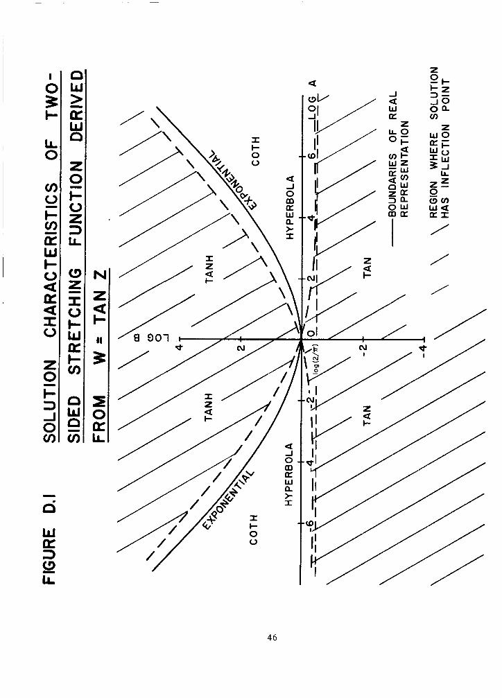
I t i s a l so instruct ive t o study the general solution ( 4 1 ) , and see how i t reduces t o d i f fe ren t real representations for various ranges of A and B . This i s carried o u t in Appendix i).
B < 1 , the solution i s a scaled portion of a tangent, while for B = 1 i t i s a scaled portion of a rectangular hyperbola. corresponding Ay given by equation (46) , the representation depends on the value of A. the solution i s a scaled portion o f a hyperbolic tangent. t h a t range the corresponding function i s the hyperbolic cotangent, while on the boundary i t i s the exponential function.
I t i s easy t o demonstrate tha t fo r
For B > 1 (and the
As shown i n Appendix il, i f exp (-Ay) < A < exp (Ay), Outside of
When A = 1 , the stretching function i s anti-symmetric, and the solution curve contains an inf lect ion point. p o i n t moves towards one end, and eventually could disappear. in Appendix D t h a t an inf lect ion point will be present i f l/cosh Ay < A < cosh Ay for B > 1 , and If B < 2 / n , the solution must always contain an inf lect ion point. Figure D.l i s a log-log plot of the B vs A plane, showing the inf lect ion point regions, as well
As A departs from one, the inf lect ion I t i s shown
cos Ax<A<l /cosAx fo r B < 1 .
17

as t h e boundaries f o r t h e v a r i o u s r e a l rep resen ta t i ons o f t h e s o l u t i o n .
Another way t o s tudy equat ion (41) i s t o f o l l o w the p a t h o f t h e s o l u t i o n i n t h e complex z-plane.
r e s u l t s p l o t t e d i n F igu re D.2. The p l o t shows c l e a r l y t h e t r a n s i t i o n f rom
one r e p r e s e n t a t i o n t o another as t h e parameters A and 6 a r e v a r i e d .
Th is i s a l s o c a r r i e d o u t i n Appendix D, w i t h t h e
A t y p i c a l s e t o f curves f o r t h e two-sided s t r e t c h i n g f u n c t i o n t ( t ) i s
shown i n f i g u r e 1 f o r so = 100, and f o r values of s1 rang ing from.1 t o 100. The f i g u r e shows t h e smooth t r a n s i t i o n f rom s o l u t i o n s c o n t a i n i n g
an i n f l e c t i o n p o i n t , f o r l a r g e sly t o those w i t h o u t an i n f l e c t i o n p o i n t
f o r smal l sl.
f o r s1 = 100 s t i l l leaves a s u f f i c i e n t number o f p o i n t s t o r e s o l v e t h e
c e n t r a l reg ion .
Note t h a t t h e h i g h c o n c e n t r a t i o n o f p o i n t s a t t he two ends
I V . A GENERAL I N T E R I O R STRETCHING FUNCTION
I n t h i s s e c t i o n we d e r i v e a general i n t e r i o r s t r e t c h i n g f u n c t i o n
<(t; si, t i ) , where si i s t h e dimensionless s lope a t t h e i n f l e c t i o n
p o i n t ti, i . e .
We l i m i t ou r c o n s i d e r a t i o n t o si >1, which i s t h e o n l y case o f p r a c t i c a l
i n t e r e s t .
odd u n i v e r s a l f u n c t i o n w(z) . As i n Sec t i on 111, t h e s imple f u n c t i o n s
s i n z and tanz a r e considered f i r s t , and c o n d i t i o n s (10) and (21) a r e
examined f o r t h e ant i -symmetr ic case ( t i = 1 /2) when si i s ve ry l a r g e .
The e v a l u a t i o n i s c a r r i e d o u t i n Appendix E, and s i n z i s found t o produce
an a p p r o p r i a t e f u n c t i o n w i t h i n v e r s e l e n g t h scales t h a t a r e l o g a r thm ica l
o f O(1). The s t r e t c h i n g f u n c t i o n t ( t ) i s a sca led p o r t i o n o f t h e i n v e r s e
h y p e r b o l i c s ine.
We again l ook f o r a f u n c t i o n which i s a sca led p o r t i o n o f an
Y
18

1
The general in te r ior stretching function fo r a rb i t ra ry ti i s readily obtained from the universal function w = sinz, by l e t t i ng z = iy . I n terms of the range Ay = y - yo, and the implicity defined E i = S ( t i ) , the f inal resu l t can be written as
I
1
I The inverse function i s
1 -1 5 = $ + sinh [(t/ti - 1 ) sinh CiAy].
The relat ion between$and t i ( fo r a given Ay) i s obtained from equation (75) by se t t ing t = 5 = 1.
I
The r e su l t can be written as
- - - 1 - cosh Ay + sinh Ay coth S i b ~ . t i
(77)
Expressing the inverse hyperbolic cotangent in terms of a logarithm, we can write the inverse of equation (77) as
Equations (76) and (78) are precisely the ones given by Thomas e t a l . ~ ( r e f . 7 )
I f s i and ti a re the given parameters, the corresponding value of Ay must be calculated. and subst i tut ing into equation (73) .
This can be done by different ia t ing equation (75) Using equation (77) t o eliminate
S i , we can write the resu l t as Ay - 1 + l / t i
1 2 - sinh Ay l2 -1 ( 7 9 )
This i s an implicit equation for Ay involving two independent parameters. If the in te r ior point i s n o t too close t o e i ther end, and the slope s i i s suf f ic ien t ly large, one can obtain a simplification. exp (-2Ay)c 51, we can approximate equation (79) a s
Assuming t h a t
19

- s i n h (Ay/2)
2Si/ \ ti ( 1 - t i ) ' AY/ 2
Equat ion (80) i s i n t h e form o f equat ion (62), and one can use t h e approximate a n a l y t i c i n v e r s i o n d e r i v e d i n Appendix B.
The spec ia l case of an ant i -symmetr ic s o l u t i o n i s obta ined by s e t t i n g
ti = S i = 1/2. The r e s u l t s ( d e r i v e d i n Appendix E) a r e
and 5 = 1/2 t 1 sinh- ' [ ( 2 t - l ) s i n h ( A y / 2 ) ] , (82 1 AY - s i n h (Ay/2) .
where si - '1/2 - AY/2
A one-sided s t r e t c h i n g f u n c t i o n i s obta ined by s e t t i n g ti = ti = 0. The r e s u l t s can be w r i t t e n as
s i n h ( t o y ) s i n h Ay t =
and < = - 1 s i n h - ' ( t s i n h Ay) , AY
- s i n h Ay AY - where Si = So -
(83)
It i s i n t e r e s t i n g t o compare t h e one-sided s t r e t c h i n g f u n c t i o n d e r i v e d
f rom t h e h y p e r b o l i c tangent (equat ions (54) t o (56)) w i t h t h e above
f u n c t i o n d e r i v e d f rom t h e h y p e r b o l i c s ine.
stand f o r t h e tangent and s i n e s o l u t i o n s , we see f rom equat ions (54 ) and
(86) t h a t f o r a g i ven so,
L e t t i n g t h e s u b s c r i p t s T arid S
2Ay, = Us.
20

The maximum inve rse l e n g t h sca le L - ' occurs a t t = 0 f o r t h e tangent s o l u t i o n , and has t h e va lue
as de f i ned by equat ion ( 2 ) t S
) ( ( L - t c max T ) = 2AyT tanh Ay, .
For t h e s ine s o l u t i o n , t h e maximum occurs a t t = 1, and has t h e va lue
1 ( ( L - tS)max)S = Ays tanh Ay, .
Thus, f o r so l a r g e enough so t h a t tanh AyT N tanh Ay, = 1, t h e two
s o l u t i o n s have t h e same maximum inve rse l e n g t h sca le .
( d c / d t ) min.occurs a t t = 1 f o r bo th s o l u t i o n s .
The minimum s lope
The r e s u l t s a r e
tanh Ay, ( (dS/d t )min)T =
AYT
tanh Ay, and ( (d</dt)rni n), =
For l a r g e so, we thus o b t a i n
hyperbo l i c s ine, f o r i d e n t i c a l c l u s t e r i n g a t t = 0.
due t o the f a c t t h a t t h e zero i n f l e c t i o n p o i n t occurs
f i r s t , and t = 0 f o r t h e second. The p a r t i c u l a r appl
determine which o f these two i s p r e f e r a b l e .
The one-sided f u n c t i o n de r i ved f rom t h e hyperbo l i c tangent thus has more
p o i n t s a t t h e unc lus te red end ( t = 1 ) than t h e one de r i ved f rom t h e he d i f f e r e n c e i s
a t t = 1 f o r t h e
c a t i o n woul d
21

V. CONCLUDING REMARKS
In this work i t has been assumed tha t the metrics and Jacobians tha t a r i s e i n the transformed equations are calculated by f i n i t e differences. I f the equation ;(t) of the 5 -coordinate curve i s known analyt ical ly , and the transformation t(€,) i s a lso given ana ly t ica l ly , then the nietrics and Jacobians can be analyt ical ly determined from the derivatives d;/dt and d t / d t . The truncation e r ro r i n the numerical calculation will then be due solely to the f ini te-difference approximations t o the derivatives o f @ w i t h respect t o 5 . the optimum transformation would be one i n which 5 varied l inear ly w i t h
@, since th i s would resu l t i n zero truncation e r rors .
When @ varies monotonically w i t h t ,
I n order t o compare transformations for the numerical and analyt ic treatment of Jacobians and metrics, consider a s t r i c t l y one-dimensional case i n which the s ingle unknown u varies monotonically w i t h distance x. Assume a highly localized in t e r io r region of rapid variation whose thickness i s proportioned t o the small parameterv. A simple exatiiple of such a solution i s
u - tanh (x/v), ( 9 3 )
where x = 0 i n the localized region. solution of Burgers' equation w i t h fixed end conditions. For the ana ly t ic treatment of Jacobians and metrics, i t follows tha t c ( x ) should be a scaled protion of the hyperbolic tangent. The analysis of Appendix E, which assumes a numerical treatment of Jacobians and metrics, shows tha t t h i s choice i s completely unsuitable, and instead favors a scaled portion o f the inverse hyperbolic sine. equation i s writ ten so tha t only derivatives of u appear, then the hyperbolic tangent transformation should lead t o a numerical solution w i t h no truncation errors . B u t the equation can a l so be written i n a form involving derivatives of several functions of u . a s t rong conservation form.
This i s actual ly the steady-state
I f the d i f fe ren t ia l
An example i s In this s i tua t ion one has several variables
22

$(<) t o be approximated by f i n i t e differences, and no s ingle transformation t (5) i s optimum for a l l of them. transformation would p u t a l l the in t e r io r grid p o i n t s inside the region o f rapid variation. There would be no points t o resolve the boundary of t h i s region. By contrast , the inverse hyperbolic sine transformation puts a suf f ic ien t number o f points outside the region of rapid variation t o resolve the complete one-dimensional region.
I f v i s very small, the hyperbolic tangent
The above discussion indicates t h a t there are special s i tuat ions and forms o f the d i f fe ren t ia l equations for which an analyt ic treatment of Jacobians and metrics can provide a desired accuracy w i t h fewer g r i d points t h a n the numerical treatment. These cases appear t o be res t r ic ted t o monotonic dis t r ibut ions t h a t can be approximated by simple analyt ic expressions. general applications of one-dimensional stretching functions , these special s i tua t ions will not be met. I t i s then best t o t r e a t the Jacobians and metrics numerically, and use the stretching functions derived in Sections I11 and IV.
For
Another assumption in the derivation of the stretching functions i s tha t the dimensionless length scale of the localized region of rapid variation could be extremely small. transformation d u d t t o be extremely large. encountered, and transformation slopes remain o f 0 ( 1 ) , then the form of the stretching function i s n o t c r i t i c a l . For example, many authors have used a scaled exponential as a one-sided stretching function. T h i s i s perfectly reasonable as long as the one-sided slope +, i s no t much larger t h a n one. B u t one can readily show t h a t the maximum inverse length scale i s exp(so) for large so.
one-sided stretching function fo r very large slopes.
This requires the dimensionless slope of the If t h i s condition i s n o t
Thus a simple exponential does n o t y ie ld a sui table
I t should be made clear t h a t Roberts was n o t the f i r s t one t o use a stretching function involving the hyperbolic tangent. ( r e f . l o ) , in an investigation of flow i n a two-dimensional channel with a rectangular cavity, used a transformation hased on the hyperbolic tangent t o transform a semi-infinite region into a f i n i t e computational region, and t o c lus te r grid po in t s a t the corners of the cavity.
Mehta and Lavan
The
23

maximum dimensionless slope, based on the lengtn of the cavity, had a value of .8664 in the i r calculations. The transformation would have been a poor one i f they had required a very large slope a t the corner, as shown in Appendix E . based on the inverse hyperbolic tangent in a study of the two-dimensional flow around an a i r f o i l . region external t o the a i r f o i l into a unit c i r c l e . The stretching function was necessary t o c lus te r points fur ther near the a i r fo i l surface ( t o capture the boundary layer) as well as the free stream ( t o overcome the stretched g r i d produced by the f i r s t transformation). the non-dimensional slopes a t the two ends were 5.77 and 27.8. In th i s instance, the use of the hyperbolic tangent was bo th appropriate and necessary, as shown by the analysis of Section 111.
The sanie authors ( r e f . 11) used a stretching function
A previous transformation had transformed the
In the i r calculation,
An important c r i te r ion i n the development of a two-sided stretching function is a continuous behavior as So and S , varied from zero t o in f in i ty . This i s necessary t o obtain smooth grids constructed algebraically using one-dimensional stretching functions. For B > 1 , the required function was found t o be based on the inverse hyperbolic tangent. the same function could be used for B < 1 , simply by interchanging cand t i n the expression. of thiswork).
A t f i r s t glance,
(This i s what was actually done in the e a r l i e r stages B u t t h i s would violate the desired continuous behavior
i n the neighborhood of B = 1 . hyperbolic tangent is the inverse tangent, which d i f f e r s from the hyperbolic tangent. se l f invert ible in th i s sense,but they do no t include the elementary functions, and therefore would n o t be useful as stretching functions. Since the inverse tangent i s no t s e l f invert ible , i t i s necessary t o use two different representations in calculating the stretching function nlrmeri cal ly .
The analyt ic continuation of the inverse
One can actually construct anti-symmetric function which are
The use of the stretching functions derived i n t h i s work requires specifying the i r slopes a t one or two points. obtained from matching slopes w i t h another function, or estimating the length scale of a localized region where an appropriate dependent variable
The values are e i the r
24
undergoes r a p i d variation. derivation of an appropriate length scale i s n o t easy, and the value t o assign t o the slope can be somewhat arbi t rary. consistent c r i te r ion i s used in assigning slope values, useful grids for numerical calculations can be generated. g r i d which was generated using the general two-sided stretching function i s found in reference 12 .
Admittedly, i n a complex s i tua t ion , the
Nevertheless, i f a
A recent example of a complex
25

X I 0
FIGURE I TWO- SIDED STRETCHING FUNCTION FOR 5i,= 100 AND DIFFERENT VALUES OF SI .
26

VI. REFERENCES
1.
2 .
3.
4.
5.
6.
7.
8.
9.
10.
11.
12.
Gough, D . O . , Spiegel, E . A . , and Toomre, J . , "Highly Stretched Meshes as Functionals of Solutions" , Proceedings of the Fourth International Conference on Numeri cal Methods i n F1 u i d Dynamics , S p r i nger-Verl ag , pp. 191-196, 1975.
Ablow, C . M . , and Schechter, S . , "Campylotropic Coordinates", J . Comp. Phys., Vol. 27(3), pp. 351-362, June 1978.
Pierson, B . L . , and Kutler, P . , "Optimal Nodal P o i n t Distribution f o r Improved Accuracy i n Computational Fluid Dynamics", A I A A J . , Vol. 18(1) , pp. 49-54, January 1980.
Thompson, J.F. , Thames, F . C . , and Mastin, C.W. , "TOMCAT- A Code f o r Numerical Generation of Boundary-Fi t t ed Curv i 1 inear Coordinate Systems on Fields Containing Any Number of Arbitrary Two-Dimensional Bodies", J . Comp. Phys., Vol. 24(3),pp. 274-302, July 1977.
Middlecoff, J .F. , and Thomas, P . D . , "Direct Control of the Grid Point Distribution i n Meshes Generated by E l l ip t i c Equations", Proceedings of the AIAA Fourth Computational Fluid Dynamics Conference , Williamsburg, Virginia, p p . 175-179, July 23-25, 1979.
Steger, J.L. , and Sorenson, R . L . , "Automatic Mesh-Point Clustering Near a Boundary i n Grid Generation With E l l i p t i c Par t ia l Differential Equations", J . Comp. Phys. , Vol. 33(3), pp.405-410, December 1979.
Thomas, P . D . , Vinokur, M . , Bastianon, R . A . , and Conti , R.J. , "Numerical Solution f o r Three-Dimensional Inviscid Supersonic Flow", AIAA J . ,
Roberts , G.O. , "Computational Meshes fo r Boundary Layer Problems" , Proceedings of the Second International Conference on Numerical Methods i n Fluid Dynamics", Springer-Verlag, pp. 171-177, 1971.
Vinokur, M . , Steger, J.L., and Pulliam, T.H. , "On Use o f Warped Spherical Coordinates t o Generate We1 1 Ordered F i n i te-Di fference Grids f o r Wing-Body Flows. Open Forum, AIAA 11th Fluid and Plasma Dynamics Conference, Sea t t l e , Washington, July 10-12, 1978.
Mehta, U . B . , and Lavan, Z., "Flow i n a Two-Dimensional Channel w i t h a Rectangular Cavity, J . Appl. Mech., Vol. 36, Series E , No. 4, pp . 897-901 , December 1969.
Mehta, U . B . , and Lavan, Z . , "Starting Vortex, Separation Bubbles and S t a l l : A Numerical Study of Laminar Unsteady Flow Around an Airfoil". J . Fluid Mech., Vol. 67(2), pp . 227-256, 1975.
Vol. 10(7), pp . 887-894, July 1972.
Lombard, C . K . , Davy, W.C. , and Green, M.J. , "Forebody and Base Region Real-Gas Flow i n Severe Planetary Entry by a Factored Implicit Numerical Method- Part I (Computational Fluid Dynamics). AIAA Paper No. 80-0065, AIAA 18th Aerospace Sciences Meeting, Pasadena, California, January 14-16, 1980.
27

APPENDIX A
EVALUATION OF ANTI-SYMMETRIC TWO-SIDED STRETCHING FUNCTIONS
I n t h i s appendix we eva lua te severa l candidates f o r an ant i -symmetr ic
two-sided s t r e t c h i n g f u n c t i o n <( t ) , where 5 and t a r e normal ized v a r i a b l e s
rang ing f rom zero t o one.
designated as
The common slopes a t t h e ends w i l l be
The t r u n c a t i o n e r r o r a n a l y s i s o f Sect ion I 1 r e s u l t s i n t h e c o n d i t i o n s
even i f B i s ve ry l a r g e . The corresponding p o r t i o n o f a u n i v e r s a l odd
f u n c t i o n w(z) ranges f rom zo = -A.,-/2 t o z1 = Az/2, where Az i s t h e t o t a l
range, and z i s e i t h e r r e a l o r pure imaginary. The s t r e t c h i n g f u n c t i o n
i s t h e r e f o r e d e f i n e d as e i t h e r
o r
L 2 W (AZ/2)
Since c o n d i t i o n s (A.2) and (A.3) a r e d i f f i c u l t t o s a t i s f y o n l y f o r ve ry
l a r g e B y we r e s t r i c t t h e a n a l y s i s t o t h e case B > l .
28

w = sinz
If we l e t z be r ea l , so tha t Az = Ax, the appropriate function B > 1 i s obtained from equation (A.5) as
I t - 7 1 - - sin [AX ( E - T ) ] 2 sin AX/^) .
Using equation (A . l )y we obtain the relat ion
tan ( A x / 2 ) A X / 2 B =
takes the form t S The inverse length scale L-l
1 L-l t< = AxItan[Ax ( 5 - 9 1 I y and has a maximum value
For large B, Ax -f T , and we obtain
(A.lO)
T h u s equation ( A . 2 ) i s violated, and the function (A.6) i s not sui table .
If we l e t z be imaginary, so t h a t Az = iAy, the appropriate function fo r B > 1 i s obtained from equation (A.4) as
- 1 = 2
sinh[Ay(t - i)] sinh (Ay/2)
Applying equation (A.l) , we obtain the relat ion
(A. l l )
29
(A.12)

The inverse length scale L-l i s now 1 t S
= 2 sinh(AY/Z) I sinh CAY ( t - 7)II L-l t c 1
1 + sinh [ Ay(t - 711
i s readily found t o be t S The maximum value of L - l
= sinh ( A Y / 2 ) . ( L - t c max
For large B , Ay/Z-+B, and we obtain
(A.13)
(A.14)
(A.15)
Since the maximum inverse length scale becomes exponentially large, the function (A. l l ) i s completely unsuitable.
w = t anz
The appropriate function for real z i s obtained from equation(A.4)as
The relat ion of B t o Ax i s obtained from equation (A.l) as
B = Ax/sin Ax.
The inverse length scale L-’ i s found t o be t S
L - ~ ~ ~ = 2 t a n ( A x / 2 ) I sin [Ax ( 2 t - 111.
For B > ~ / 2 , the maximum value of L -1 tS i s given by
l ) = 2 t a n AX/^). ( L - t c max
(A.16)
(A.17)
(A.18)
(A.19)
30

For large B y Ax + r y and equation (A.17) can be rewrit ten as
-+ (r/Z)tan (Ax/.?). Ax 2 sin ( A X / ~ ) C O S ( a ~ / 2 ) B =
We thus f ind tha t
) + 4B/al (L - t< max
and consequently the funct
(A.20)
( A . 2 1 )
on (A.16) i s a lso n o t sui tab e.
The corresponding function f o r imaginary z i s obtained from equation (A.5) as
1/2 - tanh[Ay[(-l/;)l 2 t a n h Ay/2 . t -
The parameter B i s now related t o Ay by
sinh Ay B = AY *
The inverse length scale L-l tS becomes
= 2Ay I tanh [Ay(<-1/2)] I , L-’ t 5
and has the maximum value
( L - l t S ) m a x = 2Ay t a n h (Ay/2).
For large B, equation (A.23) can be inverted approximately to
Ay+log ( 2 B log B).
( A more accurate re la t ion i s derived i n Appendix B.) For suff
( A . 2 2 )
(A.23)
(A.24)
(A.25)
yield
(A.26)
c ient ly large B , although ~y i s logarithmically of 0 (1 ) , i t i s large enough fo r tanh ( A y / 2 ) + 1 . Consequently we obtain
31

) ( L - t< max -+2Ay-2 log ( 2 8 log B ) . (A.27)
-1 T h u s L tS remains logarithmically of 0 ( 1 ) , even when B becomes extremely large. Condition (A.3) requires the determination of c-1
(For example, i f B = l lO1,(L-l t~)max = 20. ) , which i s given t S
by
(A.28)
I t follows readily f o r large B t ha t
(A.29) (C -l tS)max = (L-l t S 1 max
and condition (A.3) i s a lso sa t i s f i ed . sui table candidate f o r a s t re tching function.
The function ( A . 2 2 ) i s thus a
w = er fz
The appropriate function for real z i s obtained from equation (A.5) a s
Using equation (A. l ) , we obtain the relat ion n
The inverse length sca e L - ’ ’ ~ ~ has the simple form
1/21 Y
and has the maximum value
(A.30)
(A.31)
(A.32)
2 ) = A x . ( L - t< max (A.33)
32

Approximate inversion of equation (A.31) fo r large B r e su l t s i n
Ax2+ 4 log [2B(log B/n) 1/21 . (A.34)
i s logarithmically of 0 ( 1 ) , and can a l so show t 5 We again find tha t L-l that(T-’ )max 2 (L-’ )max. The e r ro r function i s not as simple as the hyperbolic tangent, and i s not inver t ib le . of B , the maximum inverse length scale f o r the e r ro r function i s larger than t h a t f o r the hyperbolic tangent. candidate f o r a simple, anti-symmetric, two-sided stretching function.
t5 t 5 Furthermore, f o r a given value
Thus the function (A.22) i s the best
33

APPENDIX B
I N V E R S I O N OF y = s i n h x/x
Given t h e f u n c t i o n
y = s i n h x /x ,
we seek an approximate i nve rse f u n c t i o n x = f ( y ) f o r y > l .
o f the approx imat ion w i l l be measured by c a l c u l a t i n g t h e f r a c t i o n a l e r r o r i n y, g i ven by
The accuracy
e r r o r ( y ) = -1 -1 .
An expansion f o r f ( y ) near y = 1 i s r e a d i l y obtained, bu t i t has a
smal l r a d i u s of convergence. An asymptot ic expansion f o r l a r g e y i s found t o converge ve ry s low ly . i s r e q u i r e d extends t o y -100. A maximum abso lu te e r r o r o f .0005 i s
probably s u f f i c i e n t f o r t h e numerical a p p l i c a t i o n s o f t h i s f u n c t i o n .
Hope fu l l y , these c r i t e r i a can be s a t i s f i e d by matching a p p r o p r i a t e expansions f o r smal l and l a r g e y w i t h t h e exac t s o l u t i o n a t some
i n t e r m e d i a t e p o i n t yl. Since t h e asymptot ic expansion has slow
convergence, i t w i l l a l s o be matched t o t h e exact s o l u t i o n a t another
p o i n t y2.
now be presented.
The range of y f o r which a h i g h accuracy
An o u t l i n e o f t h e d e r i v a t i o n o f t h e two expansions w i l l
For g i ven values o f x1 and x2, t h e corresponding values o f yl, y2,
(dx/dy) l , ( d x/dy ) l ,and (dx /dy ) * are ob ta ined f rom equat ion ( B . l )
by s u b s t i t u t i o n and i m p l i c i t d i f f e r e n t i a t i o n .
expansion f o r y<yI. Since y - 1 + x2/6 f o r smal l x, f ( y ) J J 6 0 f o r
y near one. I f we i n t r o d u c e t h e v a r i a b l e
2 2
We f i r s t cons ider t h e
y = y - 1 ,
we can w r i t e an expansion f o r x i n t h e form
34

The coefficients A1 and A2 are determined by inverting the expansion of equation (B.l) for small x and equating coefficients of 4. The results are
A = = -.15 1 (B.5)
and A = - 3x10⁷ 2 32x175.
2 2 By differentiating equation (B.4), we can set x, dx/dy, and d x/dy equal to their known exact values at yl. algebraic equations are readily solved for A j , A4 and A5.
The resultant three simultaneous linear
In order to obtain the expansion for y>yl,we must first determine the leading terms in the asymptotic expansion for large x. Equation (B.l) can be rewritten as
x = sinh-' (xy).
Since sinh-' z - log (2z) asymptotically for large z, we obtain the
asymp to t i c express i on
x - v+log (2x) where
v = log y.
35

S u b s t i t u t i n g t h e z e r o t h o rde r approx imat ion
X ( 0 L v (B.10)
i n t o equat ion (B.8), we o b t a i n t h e nex t approx imat ion
x ( ? v + l o g ( 2 v ) .
The f u r t h e r s u b s t i t u t i o n o f x ( l ) i n t o equat ion (B.:?,) r e s u l t s t~
v + l o g [ 2 v ( l + l o g ( 2 v ) / v ) ]
- v + l o g ( 2 v ) + l o g ( 2 v ) / v
o r x ( 2 ) - v + (1 + l / v ) l o g ( 2 v ) .
(B.11)
6.12)
The asymptot ic approx imat ion (B. 12) agrees ve ry we1 1 w i t h t h e exac t
s o l u t i o n f o r y r 1, g i v i n g a maximum abso lu te e r r o r o f ,fj2 o c c u r r i n g a t
y - 200. The n e x t h i g h e r o r d e r approx imat ion g i ves poorer r e s u l t s i n
ou r range o f i n t e r e s t . I n o rde r t o o b t a i n b e t t e r accuracy, and j o i n
t h e s o l u t i o n w i t h t h e expansion f o r smal l y, we add a polynominal i n i nve rse powers o f y.
y2, i t i s more reasonable t o d e f i n e i n s t e a d t h e v a r i a b l e
Since we w i l l a l s o match exact c o n d i t i o n s a t
w = l / y - 1/Y2. (B.13)
The expansion f o r x i s thus taken t o be
x = v + ( l + l / v ) l o g (2v) + Bo + Blw + B2w 2 + B3w3 + B4w 4 - (B. 14)
The c o e f f i c i e n t s Bo and B1 a r e determined by equat ing x and d x l d y t o
t h e i r known exac t va lues a t y2.
B4 a r e obta ined by equa t ing x, dx ldy, and d x /dy t o t h e i r known values a t
S i m i l a r l y , t h e c o e f f i c i e n t s B2, B3 and 2 2
Y l .
36

For fixed y1 and y2, as y increase above one, the e r ro r determined by equations ( B . 2 ) and(B.4) becomes posit ive, reaches a maximum, and decreases t o zero a t y l . becomes posit ive again beyond y l , reaches a maximum, decreases t h r o u g h zero, reaches a minimum (which i s negative), and increases t o zero a t y2. Beyond y2 the e r ro r grows monotonically negative. absolute e r r o r reaches a local niaximum three times i n the range
1 < y < y 2 . three maxima equal. By a t r i a l and e r ro r procedure, t h i s condition was found fo r the values x1 = 2.722567 and x2 = 6.05012, corresponding t o y, = 2.7829681 and y2 = 35.053980. e r ro r i s .000267732, which i s more than suf f ic ien t . reached a t y = 69.64. reaching .0006 a t y - 100 and .00083 a t y = 120.5. T h u s , the desired c r i t e r i a a re essent ia l ly sa t i s f i ed by the two approximations. The numerical values fo r the f ina l coeff ic ients a r e g i v e n by equations (65) and ( 6 7 ) .
Using equation (B.14), we f i n d t ha t the e r ro r
T h u s the
The optimum choice of y1 and y2 i s t ha t which makes these
The corresponding maximum absolute This value i s again
The magnitude of the e r ro r increases beyond this ,
37

APPENDIX C
I N V E R S I O N OF y = s i n x / x
Given t h e f u n c t i o n
y = s i n x / x , (C.1)
we seek an approximate i n v e r s e f u n c t i o n x = g ( y ) i n t h e range O < y < 1.
The accuracy o f t h e approx imat ion w i l l be measured by c a l c u l a t i n g t h e
f r a c t i o n a l e r r o r i n y, g i ven by
The approx imat ion i s d e r i v e d by matching a p p r o p r i a t e expansions f o r y
near zero and y near one w i t h t h e exact s o l u t i o n a t some in te rmed ia te
p o i n t yl. The d e r i v a t i o n i s b r i e f l y o u t l i n e d below.
2 2 For a g i ven xl, t h e corresponding values o f yl, (dx/dy) l ,and ( d x/dy ) 1 , a r e obta ined f rom equat ions ( C . l ) by s u b s t i t u t i o n and i m p l i c i t
d i f f e r e n t i a t i o n . equa t ion ( C . 1 ) near y = 0, as a polynomical i n powers o f T-x .
t h e i n v e r s i o n o f t h i s expansion, we take f o r an approx imat ion t h e
express ion
The approx imat ion f o r y < y l u t i l i z e s t h e expansion of Based on
(C.3) 2 2 3 4 5 6 x = ~ [ l - y+y -(l+ ~ / 6 ) y -t B4y + B5y -t B6y 3 .
2 2
The r e s u l t a n t t h r e e simultaneous By d i f f e r e n t i a t i n g equa t ion (C.3), we can s e t x , dx/dy, and d x/dy
t o t h e i r known exac t values a t y. l i n e a r a l g e b r a i c equat ions a r e r e a d i l y so lved f o r B4, B5 and B6.
equal
The approx imat ion f o r y > y l s i m i l a r l y u t i l i z e s t h e expansion o f equat ion
(C.1) near y = 1. I n t r o d u c i n g t h e v a r i a b l e
y = 1 - y ,
3c

we o b t a i n an approx imat ion i n t h e form
X =,m ( 1 + AIY + A2y2 + A3y3 + A 4 j 4 + A5j5).
The c o e f f i c i e n t s A1 and A2 obta ined f rom t h e expansion near y = 1 a r e
A, = .15
and
3x10⁷ 2 32x175 . A = -
The c o e f f i c i e n t s A3, A4 and A5 a r e ob ta ined by equat ing x, dx ldy , and
d x l d y t o t h e i r known values a t yl. 2 2
The e r r o r d e f i n e d by equat ion ( C . 2 ) reaches a l o c a l maximum between y = 0
and y = y
y = 1.
equal .
(corresponding t o y1 = .26938972).
which i s more than s u f f i c i e n t f o r numerical c a l c u l a t i o n s . The numerical
values f o r t h e f i n a l c o e f f i c i e n t s a r e g i ven by equat ions (71 ) and (72) .
and a l o c a l minimum (which i s nega t i ve ) between y = y1 and
The optimum choice o f y1 w i l l make t h e magnitudes o f these extrema
T h i s was found by t r i a l and e r r o r t o be produced by x1 = 2.428464
1 ’
The maximum absol Ute e r r o r i s .000197170,
39

APPENDIX D
SOLUTION CHARACTERISTICS OF THE TWO-SIDED STRETCHING FUNCTION DERIVED FROM w = tanz
In t h i s appendix we study the two-sided s t re tching function derived from
w = tanz,
where z i s the complex variable
z = x + iy .
If zo and zl a re the two end po in t s of the solution i n the z-plane which define the range
0, A Z = Z1 - Z
i t i s shown i n Section I11 t h a t the appropriate variables fo r the s t re tching function a re defined a s
6 = ( Z - z0)/Az
(D .3 )
(D.4)
and
t = (tanz - tanzo)/( tanzl - tanzo) 9 0 . 5 )
while the governing parameters A and B a re re la ted t o zo and z l , t h r o u g h
B = sinAz/Az (D.6)
and
coszo COSZl
A = - .
40
(D.7)

~
Using equat ion (D.3), A can a l s o be expressed i n t h e form
1/A = cosAz - tanzO sinAz . (D.8)
It i s a l s o u s e f u l t o express tanzO as a complex number i n the fo rm ~
s i n 2x0 + i s i n h 2yo
tanzO = cos 2x0 + cosh 2yo
We w i l l f i r s t s tudy t h e r e a l rep resen ta t i ons o f t he s o l u t i o n f o r
var ious ranges o f A and B. Az i s r e a l .
t h a t tanzo, z sca led p o r t i o n o f
I f B < 1, i t f o l l o w s f rom equat ion (D.6) t h a t
Using equat ions (D.8), (D.9), and (D.4), one can prove and z a re a l l r e a l . 0’ The s t r e t c h i n g f u n c t i o n i s thus a
w = t a n x . (0.10)
Th is rep resen ta t i on breaks down as B - t l , s ince Az-tO.
f rom equat ion (D.8) and (D.7) t h a t z + + I T / ~ .
r e p r e s e n t a t i o n i n t h e l i m i t by i n t r o d u c i n g
For A Z 1 , i t f o l l o w s
We can o b t a i n t h e c o r r e c t
I
- x = x TIT/2,
( D . l l )
where X30. Since t a n ( X + I T / ~ ) = - c o t X = - l / x as X - t O , i t f o l l o w s t h a t f o r B = 1 t h e s t r e t c h i n g f u n c t i o n i s a sca led p o r t i o n o f one branch o f
t h e r e c t a n g u l a r hyperbol a I
w = -l/L (D.12)
I f B > 1 , i t f o l l o w s f rom equat ion (D.6) t h a t Az i s pure imaginary,
i . e . Ax = 0.
t h e r e a l p a r t o f z i s cons tan t .
t o be pure imaginary, one can deduce f rom equat ion (D.9) t h a t x I IT/^, 0,
o r +n/2. i s x = 0, and equat ion ( D . l ) becomes
w = i t a n h y .
From equat ion (D.4) i t then f o l l o w s t h a t x = xo, so t h a t
Since equat ion (D.8) r e q u i r e d tanzO
I f A i s s u f f i c i e n t l y c lose t o one, t h e approp r ia te s o l u t i o n i i
(D.13)
41

Thus the s t r e t c h i n g f u n c t i o n i s a sca led p o r t i o n o f t he hyperbo l i c
tangent . As A depar ts f rom one, t h i s r e p r e s e n t a t i o n must break down.
One can e a s i l y show from equat ion (D.8) t h a t as A-+exp(-Ay), y o + + 03
and as A+exp(Ay), yo + - equat ion (D.13) takes t h e l i m i t i n g form
. Since l y l + a i n these two cases,
The s t r e t c h i n g f u n c t i o n then becomes a scaled p o r t i o n o f an exponen t ia l .
Th is l i m i t i s reached when B a t t a i n s the c r i t i c a l va lue
B* = s i n h l l o g A L l o g A
(D.15)
For A near one, equat ion (D.15) has t h e approximate form
l o g B* = 1/6 ( l o g A) 2 , (D.16)
w h i l e f o r A >> 1 and l / A > > 1 we o b t a i n t h e asymtot ic form
For a f i x e d A 1, as B decreases below B? t h e a p p r o p r i a t e s o l u t i o n f o r
z i s
(D.18)
The s i g n o f t h e c o r r e c t branch f o l l o w s f rom equa t ion ( D . l l ) by t a k i n g
t h e l i m i t B + l . Equat ion ( D . l ) then becomes
w = i c o t h y . (D.19)
Thus, f o r 1 < B < B * , t h e s t r e t c h i n g f u n c t i o n i s a sca led p o r t i o n o f one
branch o f t h e h y p e r b o l i c cotangent. The boundaries f o r t h e va r ious r e a l rep resen ta t i ons o f t h e s o l u t i o n art. shown i n f i g u r e D . l , which i s a l o g - l o g p l o t o f t h e B vs A plane.
42

Another i n t e r e s t i n g p r o p e r t y i s t o determine t h e c o n d i t i o n s under
which t h e s o l u t i o n curve con ta ins an i n f l e c t i o n p o i n t . Th i s i s c e r t a i n l y
t r u e f o r t h e ant i -symmetr ic curve ( A = 1 ) . As A depar ts from one, t h e i n f l e c t i o n p o i n t moves towards one end, and e v e n t u a l l y cou ld disappear.
The c r i t i c a l p o i n t i s reached when e i t h e r zl= 0 o r zo = 0. From equat ions
(D.3) and (D.7), i t f o l l o w s t h a t t h e former c o n d i t i o n occurs when
A = cosAz. (D.20)
The i n f l e c t i o n p o i n t t hus occurs a t t h e r i g h t end o f t h e curve when B a t t a i n s t h e c r i t i c a l va lue
and
Bt =/= / cosh-’ A ( A > 1 )
B+ =,/z / cos-’ A ( A < 1 ) .
(D. 21 a)
(D.21b)
For A near one, equat ion (D.21) has t h e approximate form
+ ~OCJ B = 1/3 l o g A,
w h i l e f o r A > > 1 we o b t a i n f rom equa t ion (D.21a) t h e asymto t i c form
+ l o g B + l o g 2A - l o g ( 2 l o g 2A).
+ It a l s o f o l l o w s f rom equat ion (D.21b) t h a t A + O , B
minimum value
a t t a i n s t h e
Bmin = 2 / ~ .
The c o n d i t i o n zo = 0 i s found t o occur when
(D.22)
(D.23)
(D.24)
(D.25) A = l / c o s A Z .
43

Thus t h e i n f l e c t i o n p o i n t occurs a t t h e l e f t end o f t he curve when B a t t a i n s t h e c r i t i c a l va lue
2 6- =,/l - 1/(A ) / cos-’ (1/A) ( A > 1 )
and
6- = / s l / cosh-I (1/A) ( A < l ) .
For A near one, equat ion (D.26) has the approximate form
w h i l e f o r A << 1, we o b t a i n from equat ion (D.26b) t h e asymtot ic form
(D. 26a)
(D. 26b)
(D.27)
Cond i t i on (D.24) i s again reached when A + m .
From t h e above r e l a t i o n s , one can conclude t h a t t h e s o l u t i o n curve
con ta ins an i n f l e c t i o n p o i n t un less B l i e s between B and B-.
A l t e r n a t i v e l y , an i n f l e c t i o n p o i n t w i l l be p resen t i f l /coshAy < A < coshAy f o r B > 1, and cosAx < A < l /cosAx f o r B < 1.
always occur i f B < 2 / ~ . has i n f l e c t i o n p o i n t s a r e a l s o shown i n f i g u r e D . l . r eg ions do n o t cover complete ly the reg ions where s o l u t i o n s a r e based on
t h e tangent and h y p e r b o l i c tangent.
which a s o l u t i o n curve based on t h e tangent and hyperbo l i c tangent does
n o t c o n t a i n an i n f l e c t i o n p o i n t .
t
An i n f l e c t i o n p o i n t must The reg ions o f t h e B-A Plane where t h e s o l u t i o n curve
Note t h a t these
Thus t h e r e a r e narrow ranges f o r
S t i l l another way t o s tudy t h e s o l u t i o n i s t o f o l l o w i t s pa th i n t h e
complex z-plane.
f o r constant B, as A increases f rom zero t o i n f i n i t y . It i s easy t o
show t h a t as A + O , XO+- r /2 f o r a l l s o l u t i o n s .
z + ~ / 2 f o r a l l s o l u t i o n s . The s o l u t i o n paths a r e shown i n f i g u r e D.2,
Th is i s bes t done by f i n d i n g the l o c u s o f t h e s o l u t i o n
S i m i l a r l y , as A + m ,
44

w i t h a dashed l i n e f o r B < 1 and s o l i d l i n e f o r B > 1. The d e t a i l s o f
t h e s o l u t i o n h i s t o r i e s a r e presented below.
Since z i s r e a l , t h e s o l u t i o n remains on t h e r e a l a x i s . When A = 0,
xu = -.rr/2, and x1 = -.rr/2 t Ax. (If B > &'T, x1 < 0, and t h e s o l u t i o n has no i n f l e c t i o n p o i n t ) . As A increases, bo th xo and x1 increase. ( I f B > ~ / T T , x1 = 0 and an i n f l e c t i o n p o i n t appears when A = cosAx).
When A = 1, xo = - A x / 2 , x1 = Ax/2, and we have t h e ant i -symmetr ic
s o l u i i o n . ( I f B>Z/ . r r , xo = 0 and t h e i n f l e c t i o n p o i n t d isappears
when A = l / cosAx) . When A reaches +a, x1 = v/Z, and xo = v/2 - Ax.
Wi th Az = iAy, t h e s o l u t i o n a t A = 0 has zo = -.rr/2, and z1 = - ~ / 2 + iAy.
As A increases, t h e s o l u t i o n s tays on t h e l i n e x = -v/2, and bo th yo
and y1 increase. When A = exp(-Ay), yo = y1 = +. beyond exp(-Ay), t h e s o l u t i o n r e t u r n s a long t h e imaginary a x i s , and
bo th yo and y1 decrease f rom +a. When A = l /coshAy, yo = 0, and an i n f l e c t i o n p o i n t f i r s t appears.
we have t h e ant i -symmetr ic s o l u t i o n . When A = coshAy, y1 = 0, and t h e
i n f l e c t i o n p o i n t d isappears. increases beyond exp(Ay), t h e s o l u t i o n r e t u r n s a long t h e l i n e x = n / 2 , and bo th yo and y1 inc rease f rom -m.
zo = .rr/2 - iAy.
As A increases
When A = 1, yo = -Ay/2, y1 = Ay/Z, and
- When A = exp(Ay), yo = y1 - -00. As A
When A reaches + a , z1 = .rr/2, and
B = l
When A = 0, zo = z1 = -.rr/Z.
p o i n t .
jump t o +.rr/2, where they remain as A increases t o +a.
t h e boundary between B > 1 and B < 1, t h e s o l u t i o n can occur o n l y a t these p o i n t s where t h e B > 1 and B < 1 s o l u t i o n s i n t e r s e c t .
D.2, t h e s o l i d l i n e ( B > l ) and dashed l i n e ( B ( 1 ) i n t e r s e c t p r e c i s e l y a t t h e t h r e e p o i n t s d e f i n e d above.
As A increases, t h e s o l u t i o n remains a t t h a t
When A = 1 , zo and z1 jump t o t h e o r i g i n . When A > 1 , zo and z1 Since B = 1 i s
As shown i n f i g u r e
45
N
z I- a
3
z 0
LL
ll
a
46

X
> a (0
II
a > I a, I
Q - I II V
1 )8 a a , o >
>" 8<
a I Q,
I
I
II
a .. cu
> a
I
Q) 0 V II
d a 8<
I
47

APPENDIX E
EVALUATION OF ANTI-SYMMETRIC INTERIOR STRETCHING FUNCTIONS
I n t h i s appendix we eva lua te severa l candidates f o r an ant i -symmetr ic i n t e r i o r s t r e t c h i n g f u n c t i o n < ( t ) , where 5 and t a r e normal ized
v a r i a b l e s rang ing f rom zero t o one. The s lope a t t h e m idpo in t w i l l be designated as
and o n l y t h e case B > 1 w i l l be considered. The c r i t e r i a t o be
and L ( d e f i n e d s a t i s f i e d a r e t h a t t h e i n v e r s e l e n g t h scales L - l
i n Appendix A, equat ions (A.2) and (A.3)) be o f o r d e r one, even i f B
i s ve ry l a r g e . We seek a s o l u t i o n t h a t i s a sca led p o r t i o n o f a u n i v e r s a l odd f u n c t i o n w(z). I n terms o f t h e range Az, express ions
f o r e o r t a r e g i ven by equat ions (A.4) o r (A.5).
--1 t S t S
w = tanz
I f we l e t z be r e a l , so t h a t AZ = AX, t h e a p p r o p r i a t e f u n c t i o n f o r B > 1
i s ob ta ined f rom equat ion (A.5) as
Using equat ion ( B . l ) we o b t a i n t h e r e l a t i o n
takes t h e form t E The i n v e r s e l e n g t h sca le L - '
L - l t( = 2Ax I t a n [ A x ( ( - l / Z ) ] l ,
and has a maximum value
(L- ' t S ) max = ZAX t a n ( A ~ / z ) .
(E.4)
(E.5)
43

For l a r g e B, Ax-, TI and we o b t a i n
Since t h e i n v e r s e l e n g t h sca le i s p ropor t i oned t o B, t h e f u n c t i o n (E.2)
i s n o t s u i t a b l e .
If we l e t z be imaginary, so t h a t Az = iAy, t h e a p p r o p r i a t e f u n c t i o n
f o r B > 1 i s ob ta ined f rom equat ion (A.4) as
5 - 1/2 = y$p$-#J .
Apply ing equa t ion ( E . l ) , we o b t a i n t h e r e l a t i o n
The i n v e r s e l e n g t h sca le L - l i s now t S
L- ' tS= 2 tanh (Ay/2) l s i n h [ A y ( Z t - l ) ] I ,
and has a maximum va lue
(L-lt.)max = 2 tanh (Ay/2) s i n h Ay.
For l a r g e B, Ay/2+B, tanh(A.y/2) +l, and we o b t a i n
26 ) + 2 s i n h 2 B - e . (L- t S max
( E . 7 )
(E.9)
(E.lO)
( E . l l )
Since t h e i n v e r s e l e n g t h sca le grows e x p o n e n t i a l l y w i t h B, t h e f u n c t i o n
( E . 7 ) i s complete ly unsu i tab le .
w = s i n z
The a p p r o p r i a t e f u n c t i o n f o r r e a l z i s ob ta ined f rom equa t ion (A.4)
as
49

The relat ion of B t o Ax i s obtained from equation (E . l ) as
B = = Ax/2 sin Ax/2) .
(E.12)
(E.13)
Since Ax 5 i f function ( E . 1 2 ) i s t o remain monotonic, i t follows from equation (E.13) tha t B 5 ~ / 2 . Therefore a monotonic stretching function fo r large B cannot be obtained using function ( E . 1 2 ) .
The corresponding function fo r imaginary z i s obtained from equation (A.4) as
The parameter B i s now related t o Ay by
s i n h ( Ay / 2 ) A Y / 2 - B =
The inverse length scale L-l tS becomes
L-ltS = Ay tanh [Ay(S-1/2)],
and has the maximum value
) = Ay tanh (Ay/2). ( L - t< max
For large 9, equation (E.15) can be inverted approximately t o yield
Ay+2 log (29 log 9).
For suf f ic ien t ly large B, ay i s large enough fo r tanh ( a y / 2 ) + l . Consequently we obtain
1 + A y - 2 log (29 log B ) . ( L-t<)max
50
(E.14)
(E.15)
(E.16)
(E.17)
(E.18)
(E.19)
Thus L- l tS remains l o g a r i t h m i c a l l y o f 0 (1 ) , even f o r ve ry l a r g e B. The
inve rse l e n g t h sca le I-' tS becomes
It f o l l o w s t h a t f o r l a r g e B
(E.20)
(E.21)
Since bo th i nve rse l e n g t h sca les remain o f 0 (1 ) , t h e f u n c t i o n (E.14) i s
a s u i t a b l e cand ida te f o r a s t r e t c h i n g f u n c t i o n .
51

1. Report No. NASA CR-3313
7. Authoris)
2. Government Accession No. 3. Recipient's Catalog No.
~ ~~ ~ ~~ ~ I 8. Performing Organization Report No
4. Title and Subtitle
On One-Dimensional Stretching Functions for Finite- Difference Calculations
5. Report Date
October 1980 6. Performing Organization Code
16. Abstract
Marcel Vinokur, Principal Investigator
School of Engineering
Santa Clara, California 12. Sponsoring Agency Name and Address
National Aeronautics and Space Administration Washington, D. C. 20546
,
9. Performing Organization Name and Address
Engineering and Applied Science Research University of Santa Clara
The class of one-dimensional stretching functions used in finite-difference calculations is studied. criteria for a stretching function are derived using a truncation error analysis. criteria are used to investigate two types of stretching functions. stretching function, for which the location and slope of an interior clustering region are specified. on the inverse hyperbolic sine. The other type of function is a two-sided stretching function, for which the arbitrary slopes at the two ends of the one-dimensional interval are specified. The simplest such general function is found to be one based on the inverse tangent. and greater than one was first employed by Roberts. The general two-sided function has many applications in the construction of finite-difference grids. application is found in one of the references.
For solutions containing a highly localized region of rapid variation, simple
One is an interior
The simplest such function satisfying the criteria is found to be one based
These
It was first employed by Thomas et al.
The special case where the slopes were both equal
An example of such an
10. Work Unit No.
505-31-11-06 11. Contract or Grant No.
NSG- 2086 13. Type of Report and Period Covered Contractor Report J u l y 1 , 1978 t o J u n e 30, 1979 14. Sponsoring Agency Code
7. Key Words (Suggested by Author(s) J 18. Distribution Statement
9. Security Classif. (of this report)
Unclassified
Stretching Functions, Grid Clustering, and Finite-Difference Grids
20. Security Classif. (of this page) 21. NO. of Pages 22. Price"
Unclassified 55 A04
Unclassified - Unlimited
Star Category - 64
'For sale by the National Technical Information Service, Springfield, Virginia 22161
NASA-Langley, 1980


![Robust Shrinkage Estimation of High-dimensional Covariance … · 2010-09-28 · robust covariance estimator [Tyler(1987)], which is distribution-free within the family of elliptical](https://static.fdocuments.us/doc/165x107/5ed6e20bdf0eda5e752ae517/robust-shrinkage-estimation-of-high-dimensional-covariance-2010-09-28-robust-covariance.jpg)