On non-marginal cost-benefit analysis: Abstract of Working Paper 18
28
On non-marginal cost-benefit analysis Simon Dietz and Cameron Hepburn March 2010 Centre for Climate Change Economics and Policy Working Paper No. 20 Grantham Research Institute on Climate Change and the Environment Working Paper No. 18
Transcript of On non-marginal cost-benefit analysis: Abstract of Working Paper 18
On non-marginal cost-benefit analysis
Simon Dietz and Cameron Hepburn
March 2010
Centre for Climate Change Economics and Policy
Working Paper No. 20
Grantham Research Institute on Climate Change and
the Environment
Working Paper No. 18

The Centre for Climate Change Economics and Policy (CCCEP) was established by the University of Leeds and the London School of Economics and Political Science in 2008 to advance public and private action on climate change through innovative, rigorous research. The Centre is funded by the UK Economic and Social Research Council and has five inter-linked research programmes:
1. Developing climate science and economics 2. Climate change governance for a new global deal 3. Adaptation to climate change and human development 4. Governments, markets and climate change mitigation 5. The Munich Re Programme - Evaluating the economics of climate risks and
opportunities in the insurance sector More information about the Centre for Climate Change Economics and Policy can be found at: http://www.cccep.ac.uk. The Grantham Research Institute on Climate Change and the Environment was established by the London School of Economics and Political Science in 2008 to bring together international expertise on economics, finance, geography, the environment, international development and political economy to create a world-leading centre for policy-relevant research and training in climate change and the environment. The Institute is funded by the Grantham Foundation for the Protection of the Environment, and has five research programmes:
1. Use of climate science in decision-making 2. Mitigation of climate change (including the roles of carbon markets and low-
carbon technologies) 3. Impacts of, and adaptation to, climate change, and its effects on development 4. Governance of climate change 5. Management of forests and ecosystems
More information about the Grantham Research Institute on Climate Change and the Environment can be found at: http://www.lse.ac.uk/grantham. This working paper is intended to stimulate discussion within the research community and among users of research, and its content may have been submitted for publication in academic journals. It has been reviewed by at least one internal referee before publication. The views expressed in this paper represent those of the author(s) and do not necessarily represent those of the host institutions or funders.


ON NON-MARGINALBENEFIT-COST ANALYSIS
Simon Dietz†∗ and Cameron Hepburn†‡
22 November 2010
Running title: On non-marginal benefit-cost analysis.
JEL Classification Numbers: H43, D61, Q54.
Keywords: Benefit-cost analysis, non-marginal, project appraisal, discount rate, infrastructure
investment, climate change, hydropower dam.
†Grantham Research Institute on Climate Change and the Environment, London School of Economics
and Political Science.
∗Department of Geography and Environment, London School of Economics and Political Science.
‡Smith School of Enterprise and the Environment, and New College, University of Oxford.
We thank David Anthoff, Partha Dasgupta, Francis Dennig, Christian Gollier, Chris Hope, John
Quah, Robert Ritz, Sjak Smulders, Nick Stern, seminar participants at EAERE 2009 and at the
Toulouse School of Economics, and especially Antony Millner. We would also like to acknowledge
the financial support of the Grantham Foundation for the Protection of the Environment, as well as
the Centre for Climate Change Economics and Policy, which is funded by the UK’s Economic and
Social Research Council and by Munich Re. The usual disclaimer applies.
Email for correspondence: [email protected].
Telephone: +44 207 955 7589.
Fax: +44 207 106 1241.
1

ON NON-MARGINALBENEFIT-COST ANALYSIS
Abstract
Conventional benefit-cost analysis incorporates the normally reasonable assumption that the
policy or project under examination is marginal. In particular, it is assumed that the policy or
project does not change the underlying growth rate of the economy. However, this assumption
may be inappropriate in some important circumstances, notably responding to climate change.
One example is the benefit-cost analysis of global targets for carbon emissions, while another
might be a large renewable energy project in a small economy, such as a hydropower dam.
This paper develops some theory on the evaluation of non-marginal policies and projects, with
simple empirical applications to climate change. We examine the conditions under which
evaluation of a non-marginal project using marginal methods may be wrong, and in our
empirical examples we show that both qualitative and large quantitative errors are plausible.
JEL Classification Numbers: H43, D61, Q54.
Keywords: Benefit-cost analysis, climate change, non-marginal, project appraisal, discount
rate, infrastructure investment, hydropower dam.
2
1. Introduction
Benefit-cost analysis (BCA) of major policies, programmes and projects is becoming more widely used to
inform and improve decisions (Hahn and Tetlock, 2008). In the United States and the United Kingdom,
for instance, there is now a legislative requirement to conduct BCA of significant new policies and policy
reforms, while other countries and regional organisations such as the European Commission have made
steps in the same direction (Pearce et al., 2006). In addition, there is a long tradition of BCA of major
projects by the World Bank and other multilateral financial institutions.
Conventional BCA incorporates the normally reasonable assumption that the project1 under examination
is marginal in the sense that it will not significantly change relative prices. While many projects clearly
satisfy this condition, not all of them do, and indeed it is arguable that some of the most worthwhile
projects are unlikely to be small in this sense (Hammond, 1990). Indeed, many projects are designed
precisely to change relative prices in a non-marginal way.
A rare but important category of project not only changes relative prices, but is also large enough to
shift the underlying growth rate of the relevant economy. Most notably, proposals to spend several per
cent of global GDP on the deployment of “low-carbon” technologies, such as renewable energy, smart
electricity grids and transport infrastructure, are explicitly intended to shift the global growth path by
avoiding climate change. As part of this global infrastructure investment programme, there is likely to be
a renewed impetus for large development projects in small economies, for example to generate renewable
electricity, while adaptation to climate change will require similarly large projects to, for example, store
freshwater and protect against coastal flooding. Such projects may also change the growth rate of the
small economies in which they are developed.
In their classic text on project appraisal, Dasgupta et al. (1972) largely focus on marginal, rather
than non-marginal, projects. Nevertheless they do note that different considerations may apply to large
projects:
1Henceforth we will use the word “project” to denote any change in “business as usual”, whether arising from a private-
sector or government policy, programme or project.
3

we tacitly assumed that...the proposed project is “small”, i.e. the “range” of the net benefits of
the project is small compared with the size of aggregate consumption. [Where this assumption
is untrue], it might seem plain that the EPV rule will not suffice then. One would like to
know what rule should replace it. One would also like to know whether the evaluator would
make serious errors if he stuck to the EPV rule in such cases. (p111)
While Dasgupta et al. (1972) briefly examine whether errors might occur, they do so with a simple back-
of-the-envelope calculation involving a highly specific utility function (u(c) = −10000/c) and a project
that results in a once-off cash flow. Surprisingly – and compared with the literature on BCA in the
presence only of changes in relative prices – it does not appear that a wider literature has developed to
address their questions, even though it is not particularly difficult to think of examples where the project
undertaken might have been large enough to shift the growth path of the economy (Dasgupta et al. (1972)
give the Aswan dam in Egypt as a possible example of the time). This is particularly surprising given the
problem of applying standard BCA in the presence of large changes was widely recognised at the time
the basic theory was set out: Harberger (1971) does so in his classic paper, although like Dasgupta et
al. (1972) his consideration of the issue is brief. Hammond (1990) only makes limited reference to non-
marginal projects, and only considers the impact of changes to relative prices rather than the economic
growth rate, while there is no treatment of non-marginal projects in recent texts in public economics,
such as Myles (1995), or project appraisal, such as Mishan and Quah (2007).
In the case of global carbon emissions abatement, many analyses have ignored the possibility that investing
in abatement could be non-marginal, at least in terms of how they conducted BCA. For example, Tol’s
(2005) review of the empirical literature shows that, of the 103 estimates of the shadow value of emissions
abatement he considered, 62 ignored the possibility of a shift in the growth path, because they took a
partial-equilibrium approach in which the consumption discount rate (which depends on estimated future
growth) was set irrespective of the size of future cash flows and their effect on the growth rate. That is
to say, these 62 cases carried out marginal analysis. Other analyses, such as those of Nordhaus (1994,
2008) and Stern (2007), did use a non-marginal approach, evaluating the project in a general-equilibrium
framework in which the consumption discount rate was endogenous. However, there is currently no way
of knowing whether the move from marginal to non-marginal (i.e. partial to general equilibrium) matters
4

empirically. For instance, does it matter as much as celebrated controversies in the literature, notably over
the parameters of the social discount rate? Furthermore, does it matter to project appraisal more widely,
for instance as practised by multilateral institutions such as the World Bank? Standard procedure in this
area is to apply a marginal analysis with an exogenous discount rate, irrespective of the size of a project’s
net benefits. Climate change will require an increase in the rate of energy infrastructure investment
worldwide (IEA, 2009), as well as increased investment in various forms of climate resilience such as
freshwater storage and flood defence (Agrawala and Fankhauser, 2008), including in small economies.
We can expect project appraisal to play an important role in the design and implementation of such
projects on the ground.
Hence this paper attempts to address the question of whether “serious errors” could be made by evalu-
ating non-marginal projects with conventional BCA, which uses discounted cash flow (DCF) analysis to
determine net present value (NPV). By the term “non-marginal”, we mean sufficiently large for the first-
order Taylor approximation of the utility function of aggregate consumption per capita not to hold (see
proposition 1 below). In defining non-marginal projects this way, we are interested not in the effects of
small projects on relative prices, which have been much more comprehensively explored, but on the effects
of large projects on aggregate consumption. Section 2 reviews the relevant public economic theory and
presents the result that if a project is evaluated to have positive NPV, then it is also welfare-improving,
provided that the project is marginal. It follows that if the project is non-marginal, the result may not
hold. A Taylor-series expansion provides an expression of the error involved in evaluating non-marginal
projects with DCF analysis, and comparative statics, including the impact of growing population, are
examined. These provide intuition for the circumstances in which DCF analysis may produce an error,
especially errors of large size. Section 3 then applies this theory to climate-change mitigation, using
two simple empirical examples. The first employs a well-known integrated assessment model of climate
change to estimate the value of a project to reduce global carbon emissions. The second uses data from
the World Bank to evaluate a large renewable energy project in a small economy, namely the “Nam Theun
II” hydroelectric power project in Laos. Armed with these examples, we are able to examine numerically
the sign and size of the potential error caused by evaluation of a non-marginal project using marginal
analysis. We find that it is possible for marginal BCA to provide both qualitatively and quantitatively
5

incorrect guidance, by ignoring the impacts of projects on the underlying economic growth path. Section
4 concludes.
2. Theory
2.1. Marginal BCA of a non-marginal project
A core proposition of BCA is that if DCF analysis shows that a project has positive NPV, then the
project is welfare-improving (see proposition 1). Define ∆t as the cash flows at time t from the project,
and denote the consumption discount rate by ρt. Conventional marginal BCA is conducted by DCF
analysis, which examines whether the sum of the discounted cash flows∑τt=0 ∆t(1 + ρt)
−t exceeds zero.
In contrast, full BCA calculates the true NPV by examining whether discounted utility with the project
exceeds discounted utility without it. Define ct as real, aggregate business-as-usual consumption, which
provides utility u(ct), with u′(ct) > 0 and u′′(ct) ≤ 0, and with corresponding utility discount rate δt. By
focusing on real, aggregate consumption, we abstract from issues raised by price changes, which would
require the use of a price index in order to generate a money metric (see e.g. Aronsson et al., 2004;
Weitzman, 2001). The utility discount rate and the consumption discount rate are connected by the
Euler identity (1 +ρt)−t = u′(ct)
u′(c0) (1 + δt)−t in discrete time. In continuous time with isoelastic utility this
is equivalent to ρt = δt + ηgt, where η is the elasticity of marginal utility and gt is the growth rate in
consumption (Ramsey, 1928).
Provided the project under examination is reasonably small, and the curvature of the utility function is
not too large, marginal BCA is a reasonable approximation for full BCA. Proposition 1 sets out the core
justification for the use of marginal BCA by DCF analysis in project appraisal.
Proposition 1. If u(ct + ∆t) = u(ct) + u′(ct)∆t, then
τ∑t=0
∆t(1 + ρt)−t > 0 =⇒
τ∑t=0
[u(ct + ∆t)− u(ct)](1 + δt)−t > 0 (1)
Proof. Apply the Euler equation to substitute for the consumption discount factor (1 + ρt)−t on the
left-hand side of Eq. (1). Further, provided the first-order Taylor approximation of the utility function
6

around ct is exact, so that u(ct + ∆t) = u(ct) + u′(ct)∆t, it follows that:
τ∑t=0
∆t(1 + ρt)−t =
τ∑t=0
∆tu′(ct)
u′(c0)(1 + δt)
−t =1
u′(c0)
τ∑t=0
[u(ct + ∆t)− u(ct)](1 + δt)−t (2)
As u′(c0) > 0, it follows from Eq. (2) that the implication in Eq. (1) holds.
Proposition 1 states that for marginal projects (where the first-order Taylor approximation holds), if a
project has positive NPV, it is also welfare-increasing (Little and Mirrlees, 1974). What if the first-order
approximation does not hold? The full Taylor series expansion of utility around consumption level ct is:
u(ct + ∆t) = u(ct) + u′(ct)∆t + Ω (3)
where Ω is the error in the first-order approximation, which may be given by the expression for Cauchy’s
remainder:
Ω =
∞∑j=2
uj(ct)∆jt
j!(4)
For an isoelastic utility function, u(ct) = c1−ηt /(1− η), with elasticity of marginal utility η, this error is:
Ω =
∞∑j=2
[j∏i=2
(η + i− 2)
](−1)j+1c1−η−jt
∆jt
j!(5)
For linear utility, η = 0, the error Ω = 0 and the first-order Taylor expansion is exact. At the other
extreme, as η → ∞, it is also true that Ω = 0 provided ct > 1. In other words, when the elasticity of
marginal utility, η, takes on values at the extreme ends of the range [0,∞), the error in using conventional
BCA is likely to be limited, even for a non-marginal project.
However, when η has an intermediate value, the error involved in evaluating a non-marginal project
could be substantial. Unfortunately, reasonable values of η are intermediate values; η is generally taken
to be in [0.5, 10] (Stern, 1977), and often values of [1, 4] are seen as being appropriate (Atkinson, 1970;
Johansson-Stenman et al., 2002). For instance, it is often convenient and not unreasonable to assume
logarithmic utility, with η = 1, in public economic analysis. The review of climate-change economics by
Stern (2007) did just that. Following the Stern Review, several economists (Weitzman, 2007; Dasgupta,
2007) argued that more suitable values of η were in the range [2, 4]. On the other hand, Atkinson and
Brandolini (2008) point to evidence from the literature on inequality, which supports values in the range
[0.125, 2], and Layard et al. (2008), in analysing data on subjective happiness, put η at just over unity.
7

In part, the range of estimates arises because η simultaneously represents preferences for intertemporal
substitution, aversion to risk, and aversion to (spatial) inequality with a utilitarian social welfare function
(Atkinson et. al., 2009). Nevertheless, very few economists would argue that a central estimate for η is
much below 0.5 or much above 5.
With logarithmic utility, the error in applying marginal DCF to a non-marginal project is:
Ω = −1
2
(∆t
ct
)2
+1
3
(∆t
ct
)3
− 1
4
(∆t
ct
)4
+ ... =
∞∑j=2
− ∆jt
j(−ct)j(6)
How significant could this error be? Consider a once-off, non-marginal positive cash flow at time t of
∆t. The true increase in utility derived from this cash flow is log(ct + ∆t) − log(ct). The first-order
approximation (see Eq. (3)) is ∆t/ct, and the error in that approximation is given by Eq. (6). Suppose
the cash flow ∆t from the project is positive but much smaller than business-as-usual consumption, so
that 0 < (∆t/ct) << 1, but is nevertheless large enough to be non-marginal. Then the error can itself be
approximated by the Lagrange remainder, which here is the same as the second-order term in Eq. (6),
namely: − 12 (∆t/ct)
2. The increase in utility is therefore roughly overestimated by the fraction:
12 (∆t/ct)
2
log(ct + ∆t)− log(ct)≈
12 (∆t/ct)
2
∆t/ct=
1
2
(∆t
ct
)(7)
For instance, if a project delivers a once-off benefit (∆t/ct) of 10% of current consumption, then conven-
tional DCF analysis will overestimate the actual increase in utility by approximately 5%, simply because
the marginal evaluation ignores curvature in the utility function. A 5% overestimate of benefits could
make some welfare-reducing projects appear welfare-enhancing, and vice versa for a 5% underestimate.
Of course, there are not many projects that involve increasing business-as-usual consumption by 10%
in one year. However, for projects with moderately high cash flows over several decades or more, even
annual errors of just a percentage point or two might add up to a significant overall error, and potentially
an incorrect policy prescription.
2.2. Non-marginal projects and population growth
The foregoing analysis assumed constant population. Yet many large projects are conducted in economies
with (sometimes rapid) population growth. As we will see, allowing for population growth with non-
8

marginal projects can generate some counterintuitive results. Denote population at time t as nt, and
the population growth rate as gt per period so that nt = n0(1 + gt)t. Define a “population-augmented
discount factor” βt = (1 + gt)t(1 + δt)
−t, where β0 = 1, to reflect utility discounting and population
growth combined. Finally, assume that individuals have identical utility functions, u(ct). The utilitarian
welfare increase, denoted ∆V , generated by a project with per capita cash flows of ∆t is given by:
∆V = n0
τ∑t=0
βt [u(ct + ∆t)− u(ct)] (8)
Let π denote the NPV per capita (in terms of consumption) corresponding to welfare increase ∆V , so
that π is implicitly defined by the equation:
∆V = n0 [u(c0 + π)− u(c0)] (9)
Combining Eqs. (8) and (9) and incrementing the summation index implicitly defines π as follows:
u(c0 + π) +
τ∑t=1
βtu(ct) =
τ∑t=0
βtu(ct + ∆t) (10)
Assume that costs are incurred before benefits are accrued. To fix ideas, suppose there are two periods,
t = 0, 1, where the project is represented by ∆0 < 0 < ∆1. In this case, π is implicitly defined by the
equation
u(c0 + π) + β1u(c1) = u(c0 + ∆0) + β1u(c1 + ∆1) (11)
For a marginal project in a growing economy (so c1 > c0), an increase in the concavity of the utility
function — an increase in η for an isoelastic utility function — reduces π. This is because increasing
η reduces the marginal utility of consumption in the period with high consumption (t = 1) relative
to the period with low consumption (t = 0), and the benefits ∆1 are realised in the period of high
consumption. That is to say, in a simple two-period model, provided there is positive consumption
growth g, the consumption discount factor falls with η, so future benefits are discounted more heavily
and π is lower.2 Conversely, if the sequence of project benefits and costs is reversed, so that ∆0 > 0 > ∆1,
2Note that we have abstracted here from questions of equity weighting and inequality aversion, discussed by Dasgupta
(2007), by assuming that individuals are identical.
9
then an increase in η increases π. While the latter profile of benefits and costs might be unusual (being
a disinvestment rather than the more standard investment project), in a multi-period setting it might
not be as difficult to find projects which reduce intertemporal fluctuations in consumption, at least over
a subset of time-periods.
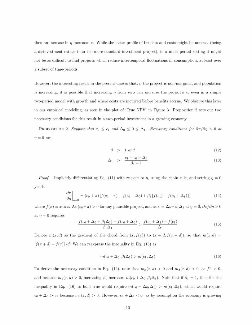
However, the interesting result in the present case is that, if the project is non-marginal, and population
is increasing, it is possible that increasing η from zero can increase the project’s π, even in a simple
two-period model with growth and where costs are incurred before benefits accrue. We observe this later
in our empirical modeling, as seen in the plot of ‘True NPV’ in Figure 3. Proposition 2 sets out two
necessary conditions for this result in a two-period investment in a growing economy.
Proposition 2. Suppose that c0 ≤ c1 and ∆0 ≤ 0 ≤ ∆1. Necessary conditions for ∂π/∂η > 0 at
η = 0 are
β > 1 and (12)
∆1 >c1 − c0 −∆0
β1 − 1(13)
Proof. Implicitly differentiating Eq. (11) with respect to η, using the chain rule, and setting η = 0
yields
∂π
∂η
∣∣∣∣η=0
= (c0 + π) [f(c0 + π)− f(c0 + ∆0) + β1f(c1)− f(c1 + ∆1)] (14)
where f(x) ≡ x lnx. As (c0 +π) > 0 for any plausible project, and as π = ∆0 +β1∆1 at η = 0, ∂π/∂η > 0
at η = 0 requires
f(c0 + ∆0 + β1∆1)− f(c0 + ∆0)
β1∆1>f(c1 + ∆1)− f(c1)
∆1(15)
Denote m(x, d) as the gradient of the chord from (x, f(x)) to (x + d, f(x + d)), so that m(x, d) =
[f(x+ d)− f(x)] /d. We can reexpress the inequality in Eq. (15) as
m(c0 + ∆0, β1∆1) > m(c1,∆1) (16)
To derive the necessary condition in Eq. (12), note that mx(x, d) > 0 and md(x, d) > 0, as f ′′ > 0,
and because md(x, d) > 0, increasing β1 increases m(c0 + ∆0, β1∆1). Note that if β1 = 1, then for the
inequality in Eq. (16) to hold true would require m(c0 + ∆0,∆1) > m(c1,∆1), which would require
c0 + ∆0 > c1 because mx(x, d) > 0. However, c0 + ∆0 < c1 as by assumption the economy is growing
10

(c1 > c0) and the project is costly (∆0 < 0). As β1 = 1 is inadequate and as md(x, d) > 0, it follows that
β1 > 1 is a necessary condition for Eq. (16) to hold and hence for ∂π/∂η > 0 at η = 0.
To derive the necessary condition in Eq. (13), compare a chord joining the point (x1, f(x1)) to (s, f(s))
with a chord joining the point (x2, f(x2)) to (s, f(s)) where s > x2 > x1. Note that m(x1, s − x1) <
m(x2, s − x2) because f ′′ > 0. Applying this, now suppose s = c0 + ∆0 + β1∆1 = c1 + ∆1, x2 = c1
and x1 = c0 + ∆0. Then for the inequality in Eq. (16) to hold would require c0 + ∆0 > c1, because
m(x1, s − x1) < m(x2, s − x2). But as noted above, the opposite is true. Hence, because mx(x, d) > 0,
c0 + ∆0 +β1∆1 > c1 + ∆1 is required, which implies ∆1 >c1−c0−∆0
β1−1 is a necessary condition for Eq. (16)
to hold and hence for ∂π/∂η > 0 at η = 0.
The intuition behind this result may be seen in three parts. First, when population growth is fast enough
that β1 > 1, project NPV per capita, π, can be extremely high. Second, in Eq. (11) the utility with the
project ∆t (on the right-hand side) is by definition equal to the utility without the project, but where
initial consumption is increased by the project NPV per capita π (on the left-hand side). If π must be
large for this equality to hold, then obviously c0 + π is also large. Third, introducing concavity in the
utility function (by increasing η from 0) leads to a greater reduction in marginal utility in periods of
relatively high consumption. When β1 > 1 and c0 + π is large, it is possible that, for the equality in Eq.
(11) to hold, π must increase to offset the relative reduction in the marginal utility of c0 + π brought
about by increasing η above zero. The relationship is not monotonic, however, and increases in η above
a certain level will have the expected effect of reducing π, because of reductions in the marginal utility
of the project benefits.
In other words, it follows from proposition 2 that an otherwise unexpected relationship between project
NPV and the elasticity of marginal utility, can emerge when population growth is fast enough that β > 1,
and when the project is sufficiently non-marginal in the sense that the benefits are large enough that
∆1 > c1−c0−∆0
β1−1 . These are not highly unusual conditions — in small developing economies it is not
implausible that the population growth rate, gt, might exceed the utility discount rate, δt, so that βt > 1.
It is also far from impossible that a project could be large enough that the second condition is satisfied.
Precisely this increasing relationship between NPV and the elasticity of marginal utility is also observed
11
in some scenarios of BCA of global carbon emissions reductions, as discussed in the following section,
and as observed in the plot of ‘True NPV’ in Figure 3.
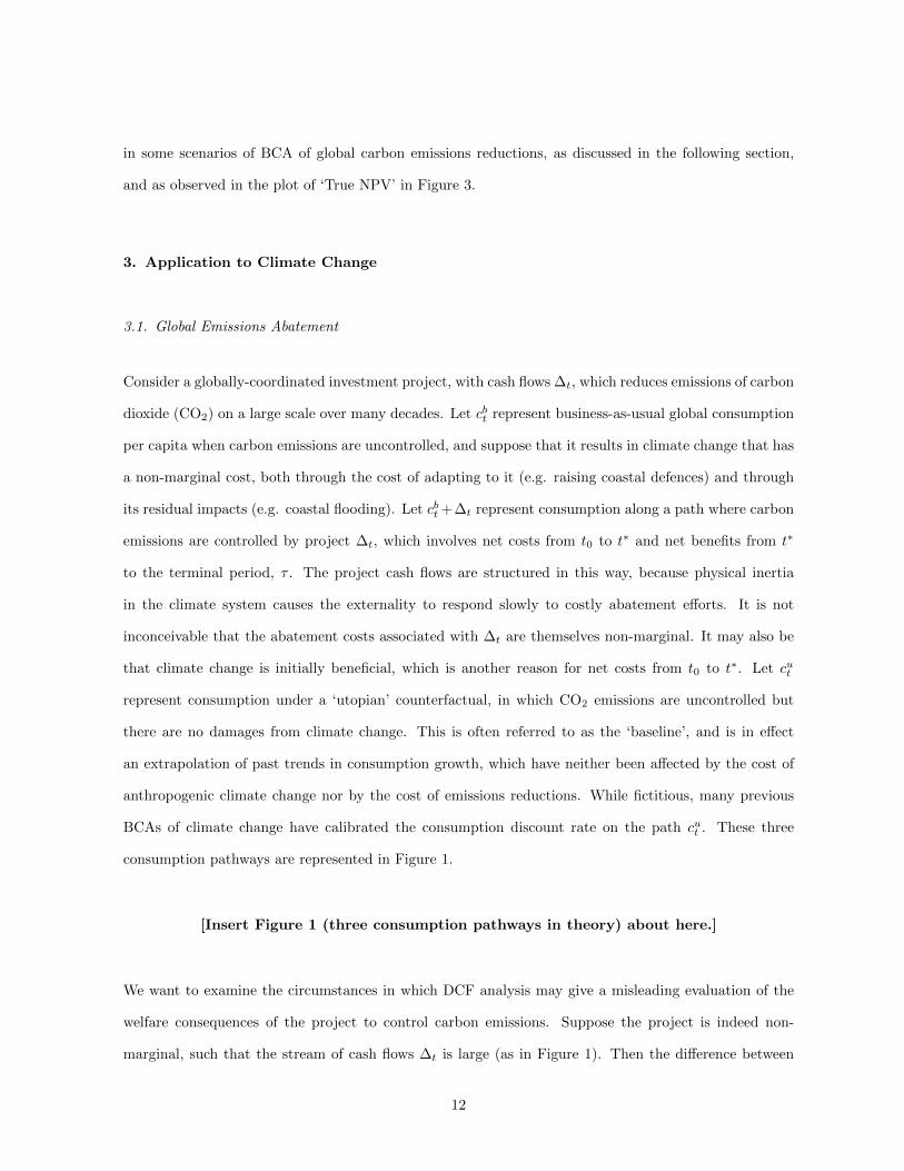
3. Application to Climate Change
3.1. Global Emissions Abatement
Consider a globally-coordinated investment project, with cash flows ∆t, which reduces emissions of carbon
dioxide (CO2) on a large scale over many decades. Let cbt represent business-as-usual global consumption
per capita when carbon emissions are uncontrolled, and suppose that it results in climate change that has
a non-marginal cost, both through the cost of adapting to it (e.g. raising coastal defences) and through
its residual impacts (e.g. coastal flooding). Let cbt +∆t represent consumption along a path where carbon
emissions are controlled by project ∆t, which involves net costs from t0 to t∗ and net benefits from t∗
to the terminal period, τ . The project cash flows are structured in this way, because physical inertia
in the climate system causes the externality to respond slowly to costly abatement efforts. It is not
inconceivable that the abatement costs associated with ∆t are themselves non-marginal. It may also be
that climate change is initially beneficial, which is another reason for net costs from t0 to t∗. Let cut
represent consumption under a ‘utopian’ counterfactual, in which CO2 emissions are uncontrolled but
there are no damages from climate change. This is often referred to as the ‘baseline’, and is in effect
an extrapolation of past trends in consumption growth, which have neither been affected by the cost of
anthropogenic climate change nor by the cost of emissions reductions. While fictitious, many previous
BCAs of climate change have calibrated the consumption discount rate on the path cut . These three
consumption pathways are represented in Figure 1.
[Insert Figure 1 (three consumption pathways in theory) about here.]
We want to examine the circumstances in which DCF analysis may give a misleading evaluation of the
welfare consequences of the project to control carbon emissions. Suppose the project is indeed non-
marginal, such that the stream of cash flows ∆t is large (as in Figure 1). Then the difference between
12
business-as-usual consumption and consumption if the project is undertaken will be large (and it follows
that the difference between both of these paths and the ‘utopian’ counterfactual will also be large).
Welfare analysis based on proposition 1 (the first-order Taylor approximation) may be unreliable because
it applies to a set of consumption discount factors along a particular path (be it cbt , cbt + ∆t, or cut ), even
though the project itself shifts the path.
Instead we must go back to the underlying welfare model and measure the difference between social
welfare on the path corresponding to the investment in emissions reductions cbt + ∆t and social welfare
on the business-as-usual path cbt . Eq. (9) provided an obvious measure of the true welfare increase of
the project ∆V , which can be rearranged for π and also Π = n0π, which denotes the true aggregate net
present (consumption) benefit from the project, given by:3
Π = n0
[u−1
(∆V
n0+ u(c0)
)− c0
](17)
Eq. (4) set out the error in project utility which arises from using the marginal method. It follows that
an equivalent expression for the error in terms of the net present consumption of the project (i.e. a money
measure), denoted ΩΠ, is the difference between Π and the sum of discounted cash flows:
ΩΠ = Π−τ∑t=0
∆t(1 + ρt)−t (18)
To explore whether “serious errors” might be made in the application of BCA to global carbon emissions
abatement, we use a so-called ‘integrated assessment model’ (IAM) of the linkages between economy and
climate. Such models have been used quite extensively over the last two decades, with the ultimate aim
of evaluating the welfare effects of planned reductions in carbon emissions. Perhaps the best known IAM
is William Nordhaus’ DICE (Nordhaus, 1994; 2008; Nordhaus and Boyer, 2000), and we use it here.
The structure and parameterisation of DICE is described in full in Nordhaus (2008). Unless explicitly
noted, we make no changes either to the model structure or to its parameter values. In brief, DICE
couples a standard Ramsey-Cass-Koopmans model of economic growth to a simple model of the climate
system. Output of a composite good is produced using aggregate capital and labour inputs, augmented
3Note that the operation of taking inverse utility requires that ∆V/n0 + u(c0) < (>)0 when η > (<)1.
13

by exogenous total factor productivity in a Cobb-Douglas production function. Production is associated
with the emission of CO2, resulting in radiative forcing of the atmosphere and an increase in global
mean temperature. The climate model couples back to the economy by means of a so-called “damage
function”, which is a reduced-form polynomial equation associating a change in temperature, as an index
of changes in a range of climatic variables, with a loss in utility, expressed in terms of equivalent output.
The damage function in DICE implicitly takes account of adaptation to climate change, which reduces
the amount of output lost for a given increase in global mean temperature, so that the representative
agent is left just to choose how much to invest in abating CO2 emissions from production.4 The model
is globally aggregated (i.e. there is a single, representative global agent), so we can simplify the analysis
and bound it more tightly with the comparative statics in section 2 by abstracting from questions of the
spatial distribution of consumption. This would be a worthwhile future extension, however, as would the
incorporation of consumption risk.
The abatement project we consider reduces emissions of CO2 with the aim of stabilising its atmospheric
stock at 1.5 times its preindustrial level, 420 parts per million (ppm). Stabilising the stock of CO2 at 1.5
times its preindustrial level has been a focus for international political and scientific discussions on climate
change, featuring prominently in, for instance, the Fourth Assessment Report of the Intergovernmental
Panel on Climate Change (IPCC, 2007). It constitutes one of the most aggressive emissions abatement
proposals currently on the table (Stern, 2007), with high costs of abatement (Nordhaus, 2008) and
potentially large avoided climate damages accordingly. Here, we use DICE to estimate the NPV of CO2
stabilisation at 420 ppm over the 200 years from 2005 to 2205.5
Figure 2 plots estimates from DICE of the NPV of the global mitigation project as a function of the
curvature of the isoelastic utility function, η. Four sets of estimates are shown, including three estimates
4As a neoclassical growth model, DICE can of course be used to optimise investment in CO2 emissions abatement, versus
investment in the composite capital good for future consumption. In line with the aims of this paper, however, we consider
exogenous policy settings, and for the sake of tractability we also specify an exogenous savings rate.5DICE is capable of running out as far as 2595, yet model predictions are especially speculative so far into the future,
and in any case Nordhaus (2008) sets up the model such that business-as-usual emissions abatement reaches 100% in the
23rd century (due to the availability of zero-carbon energy technologies at no incremental cost), so that the effect of an
explicit abatement project is most pronounced over the next 200 years or so.
14

of the DCF of the project, with the consumption discount rate in each set calibrated on DICE’s estimate
of growth along one of the three paths outlined above (i.e. cbt , cbt + ∆t and cut ). The fourth set is
our estimate of the true NPV of the project, which is the change in social welfare due to the project,
normalised to present consumption (Π in Eq. (17)).
The Figure reports results where the utility discount rate δ = 1. As we would expect, there is no difference
between DCF and true NPV — no error — when η = 0. As η increases from zero, all four estimates
of NPV fall, since per-capita consumption in the standard version of DICE is projected to grow over
the period 2005-2205, irrespective of climate change (Nordhaus, 2008). However, for our purposes the
important result is that the error ΩΠ (see Eq. (18)) increases, because the three DCF estimates fall
faster than true NPV does. Thus DCF analysis generates a fairly substantial quantitative error for small
positive values of η, although it does give the correct signal qualitatively. When η = 0.5, for example,
ΩΠ = $US 25 trillion, or in relative terms roughly 30% of the true value of the project.
For larger values of η, ΩΠ is smaller in absolute terms. When η > 1.5, DCF analysis continues to return
estimates of project value that are below its true value, but it is qualitatively correct in estimating that
the project reduces social welfare. The interesting case is when η = 1, a very common setting. Here, the
error is small in absolute terms, but DCF analysis on the commonly used path cut , as well as on the path
cbt + ∆t, is qualitatively wrong. That is to say, true NPV continues to be positive when η = 1, and yet
marginal analysis on these two paths estimates a negative discounted cash flow.
[Insert Figure 2 (NPV as a function of η) for δ = 1 about here.]
Figure 3 reports results where δ = 0. In this case, the true NPV of the project increases rapidly in the
range 0 < η < 1, while the three DCF estimates fall rapidly, thereby generating a very large quantitative
error. As η increases beyond unity, the true NPV of the project falls rapidly, reducing the error brought
about by estimating DCF. By the time η ≈ 1.5, ΩΠ is small in absolute terms. We find that the peak
in NPV is caused by population growth, as explained in section 2.2. In this case, the discount rate on
utility is sufficiently small that, when allied with population growth, the population-augmented discount
factor βt is strictly greater than unity for all t. This may be compared with the first case, when δ = 1%,
15
where we find that βt is strictly less than unity for all t.
[Insert Figure 3 (NPV as a function of η) for δ = 0 about here.]
As a final permutation of the emissions-abatement example, we make a small but significant modification
to the standard DICE model, in order to increase the difference in consumption between cbt , cbt + ∆t and
cut . In particular, we increase the important ‘climate-sensitivity’ parameter in the model. This is the
change in the global mean temperature (in equilibrium) for a doubling of the atmospheric concentration
of CO2, and it thus plays an important role in governing how much the planet is assumed to warm up
for a given pulse of emissions, and therefore how much damage will result. Standard DICE assumes that
this parameter takes the value of 3C, but IPCC (2007) estimates that the subjective probability of the
climate sensitivity being greater than 4.5C is as much as 17%. Indeed, estimates in excess of 10C have
been made (IPCC, 2007; Weitzman, 2009), although these should be considered extreme outliers. Here,
we simply double the value of the climate-sensitivity parameter to 6C and re-analyse the error in DCF
analysis (Figure 4). We also return δ to 1%.
[Insert Figure 4 (NPV as a function of η) high climate sensitivity and δ = 1.]
Figure 4 shows that it is possible for the true NPV of the project to initially increase in η with δ = 1% and
the population-augmented discount factor is less than unity. The reason is that in the simple two-period
model examined in Proposition 2 above, it was necessarily true that an investment made by the (poorer)
present for the benefit of the (richer) future increased inequality over time. In contrast, for a complex
multi-period investment such as that considered in the DICE model, it is possible that investment over
(several) earlier periods yields benefits over (many) later periods which may reduce inequality. Since η
serves as a measure of aversion to intertemporal inequality, as η increases from low levels it is possible
that such a multi-period investment is assessed to have a higher NPV because of its impact on inequality.
We conclude from these examples that marginal analysis of global carbon emissions abatement can result
in “serious errors”, both qualitative and quantitative. Many modifications of the standard DICE model
are possible, including a more pessimistic damage function (Weitzman, 2010). Often, these permutations
16
would tend to make the abatement project still larger, and would presumably reinforce our results in
terms of the possible errors in estimating NPV by DCF analysis. However, the three figures above are
sufficient to make our point.
3.2. A Large Energy Project in a Small Economy
Large infrastructure projects in small economies could also be non-marginal. Mitigation and adaptation
of climate change will require considerable infrastructure investment, including in small economies, and
it follows that economic evaluation of non-marginal projects could be an important issue. In our second
example, we estimate the error committed in carrying out DCF analysis of such a project, using as
our particular case the “Nam Theun II” hydroelectric power project in Laos, construction on which
commenced in 2005 and is due to finish shortly. According to the BCA of the World Bank (World
Bank and MIGA, 2005), which has provided loans and guarantees for the project, the net benefits of the
dam range from around -$US 240 million during the construction phase to $US 250 million during its
operation. To put these figures in context, current consumption in Laos is around $US 2.5 billion, so the
construction costs alone are in the region of 10% of national consumption.
As in our first example, let cbt represent Laos’ consumption per capita along a business-as-usual path,
which in this case is a simple projection of growth in the absence of the dam. For purposes of this analysis,
we define business-as-usual by projecting growth in Laos’ aggregate consumption, total population and
consumption per capita by a simple extrapolation of the average growth rate of GDP and population
over the period 1984-2008 as estimated in the World Bank’s World Development Indicators database
(World Bank, 2010).6 We can then use the estimated annual cash flows in World Bank and MIGA (2005)
to calculate the error in welfare evaluation. Let cbt + ∆t denote consumption per capita if the dam is
constructed, being initially lower than cbt , due to the costs of construction, but being subsequently higher,
due to the benefits of power generation. 7
6Data on consumption and saving are unavailable.7The path cut is not relevant in this case. Note also that one can conceive of several additional costs and benefits,
which are not included in the World Bank’s formal BCA, including environmental costs and the social costs of community
dislocation, as well as the potential benefits of the project to Laos’ long-run growth (i.e. the World Bank BCA only looks
17
Figure 5 plots estimates of the NPV of the dam project, again as a function of the elasticity of marginal
utility, η. Three sets of estimates are shown. These correspond to our estimate of true NPV, which is
analogous to Π in Eq. (17), and the DCF of the project, as estimated along the paths cbt and cbt + ∆t.
The utility discount rate δ = 1. It can be seen that there is again no error when η = 0, and that, when
η is increased, all three estimates of NPV decrease, due to the effect of increasing the concavity of the
utility function in a growing economy.8 But in a similar fashion to global carbon emissions abatement,
our estimate of true NPV falls more slowly than the two estimates of DCF, so that when 0 < η ≤ 1.5
a relatively large quantitative error arises, albeit the conclusion from marginal analysis is qualitatively
correct. Furthermore, when 3 ≤ η ≤ 3.75 DCF analysis is qualitatively wrong on either cbt or cbt + ∆t,
respectively estimating positive discounted cash flows when in fact the project decreases social welfare,
and vice versa.
[Insert Figure 5 (NPV of Nam Theun II) about here.]
4. Conclusion
This paper has examined the theory of non-marginal BCA, and made two simple empirical applications to
climate change. After defining non-marginality in terms of the inappropriateness of applying a first-order
Taylor approximation, theoretical expressions for the error in welfare analysis (in utility and consumption
terms) were developed. The curvature in the utility function (the elasticity of marginal utility, η) is the
source of the error, so the errors are very small for extremely low η, or extremely high η. However,
extreme values of η are not well supported by the empirical evidence, and more serious errors are theoret-
ically possible for non-marginal projects evaluated with intermediate η, for which there is good evidence.
Further, non-marginality creates the possibility of some unusual counterintuitive results when projects
are evaluated in the context of a growing population. This paper found the conditions under which an
at the ‘levels’ effect of the project). A full analysis would incorporate these factors.8Interestingly, we find that even when δ = 1, the population-augmented discount factor βt > 1 for all t. Intuitively, this
is due to Laos’ relatively rapid rate of population growth. That NPV is nevertheless decreasing in η initially, despite the
fact that βt > 1 for all t, implies that the project is insufficiently large, as defined in the necessary condition in Eq. 13.
18

increase in η can increase project NPV, in a setting without risk or distributional considerations.
The empirical part of the paper explored two climate-change mitigation projects at different scales, in
order to investigate whether conventional BCA could yield significant quantitative errors, or, perhaps
even worse, suggest outcomes which were qualitatively wrong. The first ‘project’ reduces global carbon
emissions to a low level, and was explored using the DICE integrated assessment model developed by
Nordhaus (2008). Both qualitative and large quantitative errors were found to be plausible outcomes from
the DICE model results, depending on η, the utility discount rate δ, and, as an example of dependence on
other model parameters, the climate sensitivity. The second project was the ‘Nam Theun II’ hydroelectric
power plant in Laos. Using data from the World Bank, we again found both qualitative and large
quantitative errors were possible for reasonable values of η and δ.
Following Dasgupta et al. (1972), we conclude that if there is cause to suspect a project under evaluation
is not “small”, in the sense that the range of net benefits might be a significant share of aggregate
consumption, then the NPV rule will not suffice. Instead, analysts must fall back on a general-equilibrium
model, which is capable of evaluating the underlying change in social welfare brought about by the
project. This has important implications for the evaluation of climate-change projects from the global to
the national level.
19

[1] Agrawala, S. and Fankhauser, S. (Eds.) (2008). Economic Aspects of Adaptation to Climate Change:
Costs, Benefits and Policy Instruments, Paris: OECD.
[2] Aronsson, T., Lofgren, K.-G., Backlund, K. (2004). Welfare Measurement in Imperfect Markets: a
Growth Theoretical Approach, Cheltenham: Edward Elgar.
[3] Atkinson, A.B. (1970). ‘On the measurement of inequality’, Journal of Economic Theory vol. 2, pp.
244-263.
[4] Atkinson A.B., Brandolini, A. (2009). ‘On analysing the world distribution of income’, Temi di
Discussione (Economic working papers) 701, Bank of Italy, Economic Research Department.
[5] Atkinson, G., Dietz, S., Helgeson, J. Hepburn, C. and Saelen, H. (2009). ‘Siblings, Not Triplets:
Social Preferences for Risk, Inequality and Time in Discounting Climate Change’, Economics e-
journal, 2009-26.
[6] Dasgupta, P., Marglin, S., and Sen, A. (1972). Guidelines for Project Evaluation, New York: UNIDO.
[7] Dasgupta, P. (2007). ‘Commentary: The Stern Review’s economics of climate change’, National
Institute Economic Review vol. 199, pp. 4-7.
[8] Dreze, J., Stern, N., (1987). ‘The theory of cost-benefit analysis’, in: Auerbach, A. and Feldstein,
M. (Eds.), Handbook of Public Economics, Vol. II, Amsterdam: North-Holland, pp. 909-89.
[9] Hahn, R.W., Tetlock, P.C. (2008). ‘Has economic analysis improved regulatory decisions?’, Journal
of Economic Perspectives vol. 22(1), pp. 6784.
[10] Hammond, P.J. (1990). ‘Theoretical progress in public economics: a provocative assessment’, Oxford
Economic Papers vol. 42(1), pp. 6-33.
[11] IEA (2009). World Energy Outlook 2009, Paris: IEA.
[12] IPCC (2007). Climate Change 2007: Synthesis Report, Geneva: IPCC.
[13] Johansson-Stenman, O., Carlsson, F., Daruvala, D. (2002). ‘Measuring future grandparents’ prefer-
ences for equality and relative standing’, Economic Journal, vol. 112, pp. 362-383.
20
[14] Layard, R., Mayraz, G., Nickell, S. (2008). ‘The marginal utility of income’, Journal of Public
Economics vol. 92(8-9), pp. 1846-1857.
[15] Little I.M.D., Mirrlees J.A. (1974). Project Appraisal and Planning for Developing Countries, Lon-
don: Heinemann.
[16] Mishan, E.J., Quah, E. (2007). Cost-Benefit Analysis. London: Routledge.
[17] Myles, G.D. (1995). Public Economics, Cambridge, UK: Cambridge University Press.
[18] Nordhaus, W.D. (1994). Managing the Global Commons: the Economics of Climate Change. Cam-
bridge, MA: MIT Press.
[19] Nordhaus, W.D. (2008). A Question of Balance: Weighing the Options on Global Warming Policies.
New Haven: Yale University Press.
[20] Nordhaus, W.D., Boyer, J. (2000). Warming the World: Economic Models of Global Warming.
Cambridge, MA: MIT Press.
[21] Nordhaus W.D. (2007). ‘A review of the Stern Review on the Economics of Climate Change’, Journal
of Economic Literature vol. 45, pp. 686-7.
[22] Pearce, D.W., Atkinson, G., Mourato, S. (2006). Cost-Benefit Analysis and the Environment, Paris:
OECD.
[23] Ramsey, F. (1928). ‘A mathematical theory of saving’, Economic Journal vol. 38, pp. 543-59.
[24] Stern, N. (1977). ‘Welfare weights and the elasticity of the marginal valuation of income’, in: Artis,
M., Nobay, R. (Eds.), Proceedings of the AUTE Edinburgh meeting of April 1976. Basil Blackwell.
[25] Stern, N. (2007). Stern Review: The Economics of Climate Change. Cambridge, UK: Cambridge
University Press.
[26] Tol, R.S.J. (2005). ‘The marginal damage costs of carbon dioxide emissions: an assessment of the
uncertainties’, Energy Policy vol. 33(16), pp. 2064-2074.
[27] Weitzman, M.L. (2001). ‘A contribution to the theory of welfare accounting’. Scandinavian Journal
of Economics vol. 103(1), pp. 1-23.
21
[28] Weitzman, M.L. (2007). ‘A review of the Stern Review on the Economics of Climate Change’. Journal
of Economic Literature vol. 45(3), pp. 703-724.
[29] Weitzman, M.L. (2009). ‘On modeling and interpreting the economics of catastrophic climate
change’, Review of Economics and Statistics vol. 91(1), pp. 1-19.
[30] Weitzman, M. L. (2010). ”What is the “damages function” for global warming - and what difference
might it make?” Climate Change Economics vol. 1(1), pp. 57-69.
[31] World Bank, (2010). World Development Indicators, Washington, DC: World Bank. Accessed online
on 8 November 2010.
[32] World Bank and MIGA, (2005). Project Appraisal Document on a Proposed IDA Grant (Nam Theun
2 Social and Environmental Project) in the amount of SDR13.1 million ($US20 million equivalent)
to the Lao People’s Democratic Republic and a Proposed IDA Partial Risk Guarantee in the amount
of up to US$50 million for a Syndicated Commercial Loan and Proposed MIGA Guarantees of up
to $US200 million in Lao People’s Democratic Republic and Thailand for a Syndicated Commercial
Loan to and an Equity Investment in the Nam Theun 2 Power Company Limited for the Nam Theun
2 Hydroelectric Project, Washington DC: World Bank.
22

τ
Figure 1: Three theoretical consumption pathways.
-50
0
50
100
150
200
250
300
0 0.5 1 1.5 2 2.5 3 3.5 4 4.5 5
Net
pre
sent
valu
e (
$ t
rillio
n)
DCF on cut DCF on cbt DCF on cbt + Δt True NPV
η
DCF on cut DCF on cb
t DCF on cbt + t True NPV
Figure 2: NPV of global carbon emissions abatement as a function of η for δ = 1.
23

-500
0
500
1000
1500
2000
2500
3000
0 0.5 1 1.5 2 2.5 3 3.5 4 4.5 5
Net
pre
sent
valu
e (
$ t
rillio
n)
DCF on cut DCF on cbt DCF on cbt + t True NPVDCF on cut DCF on cb
t DCF on cbt + t True NPV
η
Figure 3: NPV of global carbon emissions abatement as a function of η for δ = 0.
-500
0
500
1000
1500
2000
2500
0 0.5 1 1.5 2 2.5 3 3.5 4 4.5 5
Net
pre
sent
valu
e (
$ t
rillio
n)
DCF on cut DCF on cbt DCF on cbt + t True NPV
η
DCF on cut DCF on cb
t DCF on cbt + t True NPV
Figure 4: NPV of global carbon emissions abatement for δ = 1 with high climate sensitivity.
24

-1000
0
1000
2000
3000
4000
5000
0 0.5 1 1.5 2 2.5 3 3.5 4 4.5 5
Net
pre
sent
valu
e (
$ m
illion)
η
True NPV DCF on cbt DCF on cbt + tDCF on cbt + ΔtDCF on cb
t
Figure 5: NPV of Nam Theun II as a function of η for δ = 1.
25