
On Motion Mechanisms of Freight Train Suspension Systems
122
Southern Illinois University Carbondale OpenSIUC Dissertations eses and Dissertations 8-1-2014 On Motion Mechanisms of Freight Train Suspension Systems Dennis O'Connor Southern Illinois University Carbondale, [email protected] Follow this and additional works at: hp://opensiuc.lib.siu.edu/dissertations is Open Access Dissertation is brought to you for free and open access by the eses and Dissertations at OpenSIUC. It has been accepted for inclusion in Dissertations by an authorized administrator of OpenSIUC. For more information, please contact [email protected]. Recommended Citation O'Connor, Dennis, "On Motion Mechanisms of Freight Train Suspension Systems" (2014). Dissertations. Paper 895.
Transcript of On Motion Mechanisms of Freight Train Suspension Systems

Southern Illinois University CarbondaleOpenSIUC
Dissertations Theses and Dissertations
8-1-2014
On Motion Mechanisms of Freight TrainSuspension SystemsDennis O'ConnorSouthern Illinois University Carbondale, [email protected]
Follow this and additional works at: http://opensiuc.lib.siu.edu/dissertations
This Open Access Dissertation is brought to you for free and open access by the Theses and Dissertations at OpenSIUC. It has been accepted forinclusion in Dissertations by an authorized administrator of OpenSIUC. For more information, please contact [email protected].
Recommended CitationO'Connor, Dennis, "On Motion Mechanisms of Freight Train Suspension Systems" (2014). Dissertations. Paper 895.

ON MOTION MECHANISMS OF FREIGHT TRAIN SUSPENSION SYSTEMS
by
DENNIS MICHAEL O’CONNOR
B.S., SIUE, Mechanical Engineering, May 2004
M.S., SIUE, Mechanical Engineering, May 2007
A Dissertation
Submitted in Partial Fulfillment of the Requirements for the
PhD in Engineering Science.
Department of Engineering Science
In the Graduate School
Southern Illinois University Carbondale and Edwardsville
August 2014

ii
DISSERTATION APPROVAL
ON MOTION MECHANISMS OF FREIGHT TRAIN SUSPENSION SYSTEMS
by
Dennis Michael O’Connor
A Dissertation Submitted in Partial
Fulfillment of the Requirements
for the Degree of
Doctor of Philosophy
in the field of Mechanical Engineering
Approved by:
Albert C.J. Luo, Chair
Tsuchin Philip Chu
Fengxia Wang
Chunqing Lu
Om Agrawal
Mohammad Sayeh
Graduate School
Southern Illinois University Carbondale
August 2014

iii
ABSTRACT
ON MOTION MECHANISMS OF FREIGHT TRAIN SUSPENSION SYSTEMS
by
Dennis O’Connor
In this dissertation, a freight train suspension system is presented for all possible types of
motion. The suspension system experiences impacts and friction between wedges and bolster.
The impacts cause the chatter motions between wedges and bolster, and the friction will cause
the stick and non-stick motions between wedges and bolster. Due to the wedge effect, the
suspension system may become stuck and not move, which cause the suspension lose functions.
To discuss such phenomena in the freight train suspension systems, the theory of discontinuous
dynamical systems is used, and the motion mechanism of impacting chatter with stick and stuck
is discussed. The analytical conditions for the onset and vanishing of stick motions between the
wedges and bolster are presented, and the condition for maintaining stick motion was achieved as
well. The analytical conditions for stuck motion are developed to determine the onset and
vanishing conditions for stuck motion. Analytical prediction of periodic motions relative to
impacting chatter with stick and stuck motions in train suspension is performed through the
mapping dynamics. The corresponding analyses of local stability and bifurcation are carried out,
and the grazing and stick conditions are used to determine periodic motions. Numerical
simulations are to illustrate periodic motions of stick and stuck motions. Finally, from field
testing data, the effects of wedge angle on the motions of the suspension is presented to find a
more desirable suspension response for design.

iv
DEDICATION
This dissertation is dedicated to my two sons Rylan and Nevan O’Connor. The heart of this
research is to understand the how and why two systems interact and behave. Indeed, some of my
greatest insights into this work have come from raising two boys. How at times they can bring
world peace and at other times world destruction, I have often considered through laughing tears
and telling headaches. More importantly though, they have sustained my balance and given me
an immeasurable richness in life. May they be inspired and tireless in their own pursuits of the
stars. Having asked me repeatedly “Daddy, when will you finish?” I owe the completion of this
work to their infinite charm and persuasion.
You two are my world.

v
ACKNOWLEDGMENTS
First and foremost, I would like to thank Dr. Albert Luo. For the depth of knowledge and
life philosophy he has bestowed on me, I am forever grateful and indebted. Furthermore, this
work was strictly made possible by the teachings and guidance of Dr. Luo. From his
breakthrough research on discontinuous dynamical systems, a simplified but incredibly realistic
mechanical model was achieved for train suspension. For both helping with the completion of
this work and new insights into the rule of mathematics, I owe special thanks to Dr. Chunqing
Lu. I would also like to thank my thesis advisory committee members: Dr. Fengxia Wang, Dr.
Philip Chu, Dr. Om Agrawal, and Dr. Mohammed Sayeh. And to Amsted Rail for initiating this
project and providing useful tips and help to yield a more accurate mechanical model.
For the unyielding support throughout my life and, in particular, during my PhD study, I
thank my parents Daniel and Lois O’Connor. Through endless homemade pies and hours of
babysitting, they have afforded me the time and peace of mind to complete this work. And to my
brothers and many friends, who distracted, encouraged, and helped me along the way, thank you
all.

vi
TABLE OF CONTENTS
CHAPTER PAGE
APPROVAL ................................................................................................................................... ii
ABSTRACT ................................................................................................................................... iii
DEDICATION ............................................................................................................................... iv
ACKNOWLEDGMENTS ...............................................................................................................v
LIST OF TABLES ....................................................................................................................... viii
LIST OF FIGURES ........................................................................................................................ ix
CHAPTER I - INTRODUCTION ....................................................................................................1
1.1 Bibliography ...................................................................................................................1
1.2 Physical Model ...............................................................................................................4
1.3 Objectives ......................................................................................................................5
1.4 Layout ............................................................................................................................6
1.5 Significance of Research ................................................................................................7
CHAPTER II - MECHANICAL MODEL .......................................................................................8
2.1 Equations of Motion ......................................................................................................8
2.2 Absolute Motion ..........................................................................................................13
2.3 Relative Motion ...........................................................................................................20
CHAPTER III – MOTION MECHANISMS .................................................................................23
3.1 Stuck and Sliding Conditions ......................................................................................23
3.1 Free-Flight and Stick Motions .....................................................................................33
CHAPTER IV - Motion Description .............................................................................................40
4.1 Switching Sets and Basic Mappings ...........................................................................40
vii
4.2 Algebraic Equations for Mappings ..............................................................................44
4.3 Mapping Structures .....................................................................................................47
4.3 Bifurcation Scenario ...................................................................................................48
CHAPTER V - General Results .....................................................................................................53
5.1 Periodic Motion ...........................................................................................................53
5.2 Stability ........................................................................................................................54
5.3 Impacting Chatter Prediction .......................................................................................56
5.4 Impacting Chatter with Stuck and Stuck Prediction ....................................................62
5.5 Numerical Simulations of Periodic Chatter .................................................................68
5.6 Numerical Simulations of Chatter with Stick and Stuck Motion ................................72
CHAPTER VI - Wedge Angle Investigation .................................................................................79
6.1 Field Data Results ........................................................................................................79
6.2 Analytical Prediction ....................................................................................................80
6.3 Numerical Simulation ..................................................................................................86
6.4 Work Dissipation by Friction .......................................................................................91
CHAPTER VII - SUMMARY .......................................................................................................96
REFERENCES ..............................................................................................................................98
APPENDIX A - General Solutions ..............................................................................................100
APPENDIX B - Numerical Simulation Algorithm ......................................................................103
APPENDIX C - Jacobean Matrix ................................................................................................104
VITA ..........................................................................................................................................108

viii
LIST OF TABLES
TABLE PAGE
Table 4.1. Summary of excitation frequency for impacting chatter with stick. .............................51
Table 4.2. Summary of excitation frequency for impacting chatter with stuck. ............................52
Table 6.1. Summary of excitation frequency for impacting chatter with stick. .............................85
Table 6.2. Tabulated values of displacement acceleration and work .............................................95

ix
LIST OF FIGURES
FIGURE PAGE
Figure 1.1. A mechanical description of freight train suspension ....................................................4
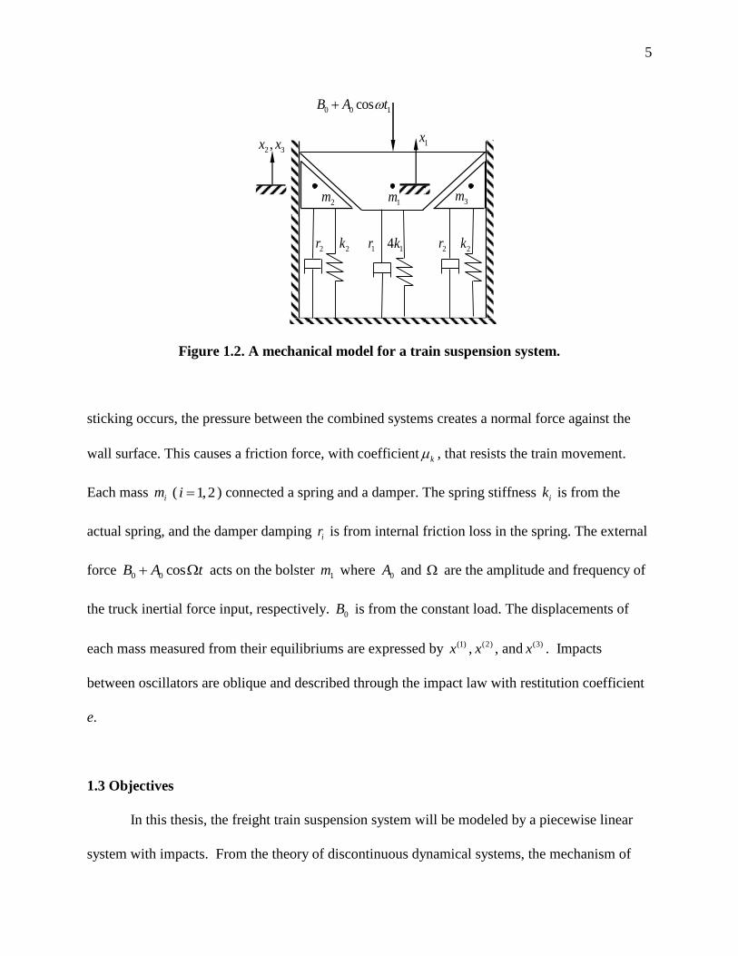
Figure 1.2. A mechanical model for a train suspension system. ......................................................5
Figure 2.1. Free body diagram of wedge and bolster not in contact. ...............................................8
Figure 2.2. Free body diagram of wedge and bolster in contact ....................................................10
Figure 2.3. Friction model varying with time. ..............................................................................12
Figure 2.4. Free-flight domain and boundary: (a) bolster and (b) wedges. ....................................14
Figure 2.5. Phase plane domains and boundaries for stick motion: (a) bolster and (b) wedges ....16
Figure 2.6. Phase plane domains for mixed free-flight and stick motion: (a) bolster (b) wedge ...18
Figure 2.7. Phase plane partition in the relative reference frame: (a) bolster and (b) wedges .......22
Figure 3.1. Passable flow illustration on (a) ( )
32
i and (b) ( )
23
i . .................................................26
Figure 3.2. Stuck motion illustration on (a) ( )
32
i and (b) ( )
23
i ...................................................29
Figure 3.3. Vanishing of stuck motion: (a) from ( )
32
i to ( )
2
i and (b) form ( )
23
i to ( )
3
i .........32
Figure 3.4. Free-flight grazing illustration on (1)
1 . ...................................................................34
Figure 3.5. Stick motion on (1)
13 in the phase plane of bolster. ...................................................36
Figure 3.6. Stick motion vanishing illustration on (1)
21 ...............................................................37
Figure 3.7. Grazing motion illustration for stick vanishing at ( )
21
i ............................................39
Figure 4.1. Mapping: (a) stick and (b) stuck motion .....................................................................41
Figure 4.2. The free flight to impacting chatter map 5P ................................................................43
Figure 4.3. Mixed domain mappings with free-flight, chatter, and stick switching. .....................44
x
Figure 4.4. Bifurcation scenario for switching: (a) phase and (b) displacement ...........................49
Figure 4.5. Bifurcation scenario for switching: (a) bolsters velocity and (b) wedge velocity .......50
Figure 5.1. Analytical prediction of (a) switching phase and (b) displacement for 5P .................58
Figure 5.2. Analytical prediction of switching velocities for 5P ...................................................59
Figure 5.3. Analytical eigenvalues (a) 1,2,3,4Re( ) and (b) 1,2,3,4Im( ) for 5P ..............................60
Figure 5.4. Magnitude of eigenvalues for (a) 5P and (b)
55P .........................................................61
Figure 5.5. Analytical prediction of (a) switching phase (b) zoomed (1.35,1.40) portion for
chatter with stick and stuck .........................................................................................63
Figure 5.6. Analytical prediction of (a) switching displacement and (b) zoomed (1.35,1.40)
portion for chatter with stick and stuck. .......................................................................64
Figure 5.7. Analytical prediction of (a) switching velocity (1)y and (b) zoomed (1.35,1.40)
portion for chatter with stick and stuck. .......................................................................65
Figure 5.8. Analytical prediction of (a) switching velocity (2)y and (b) zoomed portion for
chatter with stick and stuck ..........................................................................................66
Figure 5.9. Magnitude of eigenvalues for chatter with stick and stuck .........................................67
Figure 5.10. Displacement and velocity response for simple impacting chatter 5P .......................69
Figure 5.11. Phase plane trajectories for simple impacting chatter 5P ...........................................70
Figure 5.12. Relative force and jerk response for simple for simple impacting chatter 5P ............71
Figure 5.13. Displacement and velocity response for impacting chatter with stick and stuck
Motion 215 4306P ......................................................................................................................74
xi
Figure 5.14. Acceleration and Normal Force response for impacting chatter with stick and stuck
motion 215 4306P ............................................................................................................75
Figure 5.15. Phase plane trajectories of bolster and wedge for impacting chatter with stick and
stuck motion 215 4306P ...................................................................................................76
Figure 5.16. First and second order stuck condition function for motion 215 4306P ..........................77
Figure 5.17. Relative force and jerk time-history for 215 4306P .........................................................78
Figure 6.1. Field data of wedge vertical displacement and wedge-bolster relative movement,
Amsted Rail Inc ............................................................................................................80
Figure 6.2. Field data of wedge normal force time-history and wedge normal force versus
displacement, Amsted Rail Inc .....................................................................................81
Figure 6.3. Analytical prediction of switching phase and displacement. .......................................83
Figure 6.4. Analytical eigenvalues (a) 1,2,3,4Re( ) and (b) 1,2,3,4Im( ) . .......................................84
Figure 6.5. Displacement and velocity response for 210P ...............................................................87
Figure 6.6. Acceleration response and phase plane trajectory for 210P ..........................................88
Figure 6.7. Wedge normal force time-history and wedge normal force versus displacement for
210P ...............................................................................................................................89
Figure 6.8. First and second order stuck condition function for 210P ............................................90
Figure 6.9. Friction force response for 210P ....................................................................................92
Figure 6.10. Friction force versus displacement for (a) negative velocity and (b) positive velocity,
0.654rad .............................................................................................................94

1
CHAPTER I
INTRODUCTION
In this chapter, a literature review of research on train suspension systems describes the
approaches and progress made in the work of modeling and understanding such systems. While
considerable advancements have been made in passenger train suspension systems, far less
developments have been realized in freight train suspension systems. Herein, a mechanical
model of the freight train suspension system is introduced for investigation. Through this model,
the dynamic behaviors of the current suspension system may be better understood and
improvements to the overall system realized.
1.1 Bibliography
Train suspension systems are for the comfort and stability of train locomotion, and an
effective suspension system is necessary for safety and reliability. With the advancements in
control theory and suspension technology, significant improvements have been made for
passenger trains. Shieh et al. (2005) developed the optimal control to the passive suspension
system of the light rail train using evolution algorithms. A train model with nine degrees of
freedom was introduced and a stochastic optimization algorithm was used to optimize the
suspension system parameters. Gottzein & Lange (1975) modeled the wheel-less high-speed
passenger train to design the magnetic levitation suspension system. For the riding comfort of
trains, Wu & Yang (2003) investigated the dynamic responses of trains moving over simply
supported bridges through the development of a mechanical model including impact. Sayyaadi &
Shokouhi (2009) introduced a system with seventy degrees of freedom for the rail-vehicle

2
suspension including a nonlinear air-spring damper. Experimental studies showed the
effectiveness of the suspension system and the relevance of the mechanical model. Other
research has considered the environmental impact of moving trains. Karlstrom (2006) developed
an analytical model for the train-induced ground vibrations and simulated the vibration responses
at various train speeds. Using a finite element approach, Ju & Lin (2008) investigated the ground
vibration from high-speed trains and compared the results with experimental measurements.
On the other hand, less advancement has been attained for the suspension system of freight
trains. Indeed, the ubiquitous wedge based friction-damped suspension system for heavy haul
freight trains has not been changed too much in the past century while speed and cargo demands
have increased greatly. The freight train suspension system uses friction damping in which pairs
of wedges perform a force transmission of the track disturbance onto the side frame wall of the
train undercarriage. Gardner & Cusumano (1997) discussed the differences between the variable-
damping and constant-damping friction wedge model as well as the wedge model used in the
dynamic train simulator software NUCARS®. Kaiser et al. (2002) considered a piecewise
smooth wedge model with dry friction and gave parameter studies focused on the slip-stick
phenomena. In that model, the wedge and bolster remain in contact, and periodic motions were
found through numerical and harmonic balance methods. The separation of the wedges and
bolster with the directional change of the friction is allowed, and the train suspension system can
be investigated with a piecewise linear model including friction and impact.
The impacts between two masses in the train suspension system are similar to the dynamics
of gear transmission. Herein, the gear dynamics is reviewed herein to help us work on the
dynamics of train suspension systems. For instance, Pfeiffer (1984) presented an impact model to
investigate dynamics of gear transmissions, and the regular and chaotic motions in the gear box

3
were investigated in Karagiannis & Pfeiffer (1991). One also used a piecewise linear model to
investigate the dynamics of gear transmission systems (e.g., Comparin & Singh, 1989;
Theodossiades & Natsiavas, 2000). To model vibrations in gear transmission systems, Luo &
Chen (2005) used an impact model of two oscillators, and the local singularity theory in Luo
(2005) was used for grazing and chaotic motions. Luo & O’Connor (2009) discussed the
mechanism of impacting chatter with stick, and the analytical prediction of periodic chatter with
and without stick was completed. The train suspension system is a dynamical system of three
bodies with impact and frictions. One worked on nonlinear dynamics of two systems connected
with the friction for many years. For instance, Hundal (1979) examined the response of a base
excited system with Coulomb and viscous friction, and Feeny (1992) studied a non-smooth
Coulomb friction oscillator. Shaw & Holmes (1983) studied nonlinear dynamics of a piecewise
linear oscillator, and Shaw (1986) investigated a piecewise linear oscillator with dry friction. Luo
& Gegg (2006) developed the stick and non-stick force criteria for the friction induced oscillator.
Combining the friction and impact phenomena, Hinrichs et al. (1997) investigated the dynamics
of a system undergoing friction as well as impact. An experimental investigation of stick-slip
dynamics in a friction wedge damper was carried out in Chandiramani et al. (2006).
In this paper, a simple model for the train suspension system will be presented. The bolster
and two wedges will be considered to be independent, and impacts between the wedge and
bolster occur at different locations. When sticking together, the combined wedge and bolster
system will experience friction. This train suspension system with friction and impact will be
modeled. Following the ideas of Luo & O’Connor (2009), the global nonlinear behaviors of such
a suspension system will be discussed and parameter maps will be presented. Numerical
illustrations will be given for parameter characteristics of impacting chatter with/without stick for

4
the train suspension system. The theory for discontinuous dynamical systems can be found from
Luo (2009) and (2012).
1.2 Physical Model
To model the freight train suspension system, consider the general configuration of the train
suspension system, as shown in Figure 1.1. A major bracket known as the bolster is anchored to
the bottom of the train. The bolster rests within the side arm on a set of springs and a pair of
wedges. The wedges create friction dampening as they are pressed down and against the wall of
the side arm. Since the tracks may not be perfectly level, the track is described by the curve
underneath the wheels. Note, each train car has two complete sets of the suspension system
described in Figure 1.1. Further, due to symmetry, only one side of the suspension system is
shown.
Consider a periodically forced oscillator acted upon by a pair of secondary oscillators, as
shown in Figure1.2. The primary mass represents the bolster on the train suspension system,
while the pair of secondary masses represents the wedges used for the friction damping.
Interaction between the bolster and wedges causes impacting and sticking together. When
Bolster
Wheels
Track
Train (Friction Wedges) (Side Frame)
Figure 1.1. A mechanical description of freight train suspension.
5
1m 2m 3m
2r 2k 2r 2k 1r 14k
2 3,x x 1x
0 0 1cosB A t
Figure 1.2. A mechanical model for a train suspension system.
sticking occurs, the pressure between the combined systems creates a normal force against the
wall surface. This causes a friction force, with coefficient k , that resists the train movement.
Each mass im ( 1,2i ) connected a spring and a damper. The spring stiffness ik is from the
actual spring, and the damper damping ir is from internal friction loss in the spring. The external
force 0 0 cosB A t acts on the bolster 1m where 0A and are the amplitude and frequency of
the truck inertial force input, respectively. 0B is from the constant load. The displacements of
each mass measured from their equilibriums are expressed by (1)x , (2)x , and (3)x . Impacts
between oscillators are oblique and described through the impact law with restitution coefficient
e.
1.3 Objectives
In this thesis, the freight train suspension system will be modeled by a piecewise linear
system with impacts. From the theory of discontinuous dynamical systems, the mechanism of

6
impacting chatter with stick and stuck will be investigated, and the onset and vanishing
conditions of such motions will be developed. The condition for maintaining stick and stuck
motion in such a suspension system will be discussed. Motion mappings will be introduced first
based on the separation boundaries, and then from the basic mappings, the mapping structures
will be developed for periodic motions. Further, the analytical prediction of periodic motions
pertaining to impacting chatter with stick and stuck can be completed, and the corresponding
local stability and bifurcation of the periodic motion will be analyzed. Analytical conditions will
be employed to complete the bifurcation analysis, and numerical simulations will be carried out
for illustration of periodic motions and stick criteria.
1.4 Layout
To begin, this thesis conducts a literature survey on related and pertinent works of train
suspension systems. Also, a mechanical model for train suspension is developed based on a
simplification of the said mechanical system. In Chapter 2, a mathematical description of the
train suspension system will be given. Additionally, the equations of motion based on the
absolute and relative frames will be developed on the different domains. In Chapter 3, the stick,
stuck, and grazing criteria for such a suspension system will be derived from the singularity
theory of discontinuous systems on the boundary. In chapter 4, the basic mappings will be
introduced for developing the mapping structure of periodic motion. Based on the mapping
structure, the periodic motion can be predicted analytically. The corresponding stability and
bifurcation analysis will be carried out in Chapter 5. For illustration of the analytical conditions,
the displacement response, velocity response, and phase planes of periodic motions in such a
suspension system will be presented. In Chapter 6, field data from Amsted Rail is implemented

7
to consider realistic suspension parameters. In addition, an investigation into wedge angle
influence of system response through analytical prediction will be conducted. Finally, in Chapter
7 the summary of this thesis project will be given.
1.5 Significance of Research
The simplified train suspension model in Figure 1.2 is investigated in order to better
understand the vibration and dynamic phenomena experienced during train locomotion. More
specifically, the suspension system discussed herein is investigated so that the underlying
behavioral characteristics of train suspension can be identified and controlled to avoid derailment
or unsafe vibration. Parametric investigations will provide insights into motion mechanisms for
impacting chatter with stick and stuck motion. Moreover, the analytical conditions of such
motion phenomena may provide efficient methods to catch the motion switching, and this will
give a good physical interpretation of vibration in such a train suspension system. An
investigation into the influence of wedge angle can help design future suspension systems to
avoid undesirable suspension behavior. Finally, with such a mechanical model, vibration and
dynamic behavior of the train can be adjusted through the operating conditions and a better
performance may be achieved.
8
CHAPTER II
MECHANICAL MODEL
In this chapter, the mathematical model of the freight train suspension system described
in Chapter 1 will be developed. From Newton’s laws, the equations of motion are introduced to
describe the different types of motion. Based on the regions for each type of motion, domains and
their respective boundaries will be defined. Importantly, the boundaries represent a discontinuity
and must be considered carefully to determine how motion may interact in such proximity. To
this end, the corresponding state variables for the equations of motion in the absolute and relative
reference frames will be defined and boundaries described mathematically.
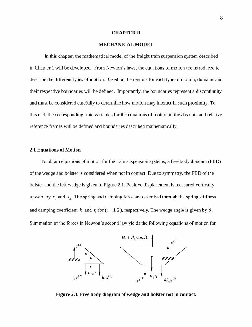
2.1 Equations of Motion
To obtain equations of motion for the train suspension systems, a free body diagram (FBD)
of the wedge and bolster is considered when not in contact. Due to symmetry, the FBD of the
bolster and the left wedge is given in Figure 2.1. Positive displacement is measured vertically
upward by 1x and 2x . The spring and damping force are described through the spring stiffness
and damping coefficient ik and ir for ( 1,2i ), respectively. The wedge angle is given by .
Summation of the forces in Newton’s second law yields the following equations of motion for
(2)
2k x
0 0 cosB A t
(2)
2r x (1)
14k x (1)
1r x 1m g 2m g
(2)x
(1)x
Figure 2.1. Free body diagram of wedge and bolster not in contact.
9
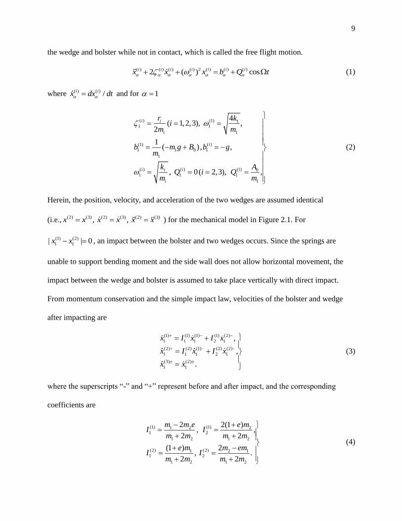
the wedge and bolster while not in contact, which is called the free flight motion.
( ) ( ) ( ) ( ) 2 ( ) ( ) ( )2 ( ) cosi i i i i i ix x x b Q t (1)
where ( ) ( ) /i ix dx dt and for 1
( ) (1) 11 1
1
(1) ( )
1 1 0 1
1
( ) ( ) (1) 01 1 1
1
4( 1,2,3), ,
2
1( ) , ,
, 0 ( 2,3), ,
i i
i
i
i ii
i
r ki
m m
b m g B b gm
k AQ i Q
m m
(2)
Herein, the position, velocity, and acceleration of the two wedges are assumed identical
(i.e., (2) (3) ,x x (2) (3) ,x x (2) (3)x x ) for the mechanical model in Figure 2.1. For
(1) (2)
1 1| | 0x x , an impact between the bolster and two wedges occurs. Since the springs are
unable to support bending moment and the side wall does not allow horizontal movement, the
impact between the wedge and bolster is assumed to take place vertically with direct impact.
From momentum conservation and the simple impact law, velocities of the bolster and wedge
after impacting are
(1) (1) (1) (1) (2)
1 1 1 2 1
(2) (2) (1) (2) (2)
1 1 1 2 1
(3) (2)
1 1
,
,
.
x I x I x
x I x I x
x x
(3)
where the superscripts “-” and “+” represent before and after impact, and the corresponding
coefficients are
(1) (1)1 2 21 2
1 2 1 2
(2) (2)1 2 11 2
1 2 1 2
2 2(1 ), ,
2 2
(1 ) 2, .
2 2
m m e e mI I
m m m m
e m m emI I
m m m m
(4)

10
0N
(2)
2k x
N
kF
N
0 0 cosB A t
(2)
2r x (1)
14k x (1)
1r x
1m g 2m g
(2)x (1)x
Figure 2.2. Free body diagram of wedge and bolster in contact.
Consider the wedge and bolster to remain in contact, which is called the stick motion. The
free body diagram for this scenario is given in Figure 2.2. The normal force N is the contact
force between the wedge and bolster. Herein, it is assumed that the wedge and bolster make a
point contact and no slipping occurs. Subsequently any friction force acting between the wedge
and bolster can be neglected. However, as a result of the wedge angle , there is an additional
normal force 0N defining the contact force between the side wall and wedge. This normal force
creates a kinetic friction force fF as defined in Eq.(5).
0 2
2 0 0 2
0 2
[0, ),
( ) [ , ] 0,
( ,0].
k
f k k
k
N x
F x N N x
N x
(5)
Further, the normal force 0N is related to the normal force N , i.e.,
0 cos .N N (6)
The total forces in Figure 2.2 with Eqs.(5) and (6), the equations of motion for the combined
mass system for 1,2i and 2,3 is given by
( ) ( ) ( ) ( ) 2 ( ) ( ) ( )2 ( ) cosi i i i i i ix x x b Q t (7)
11
where
( ) ( ) ( )1 2 1 2 0
1 2 1 2 1 2
( ) 1 2 0
(2)
1 2
4, , ,
( ) 2sin, .
sin cos sgn( )
i i is s
s s s
i ss
s k
r r k k AQ
m m m m m m
m m g Bb
m m x
(8)
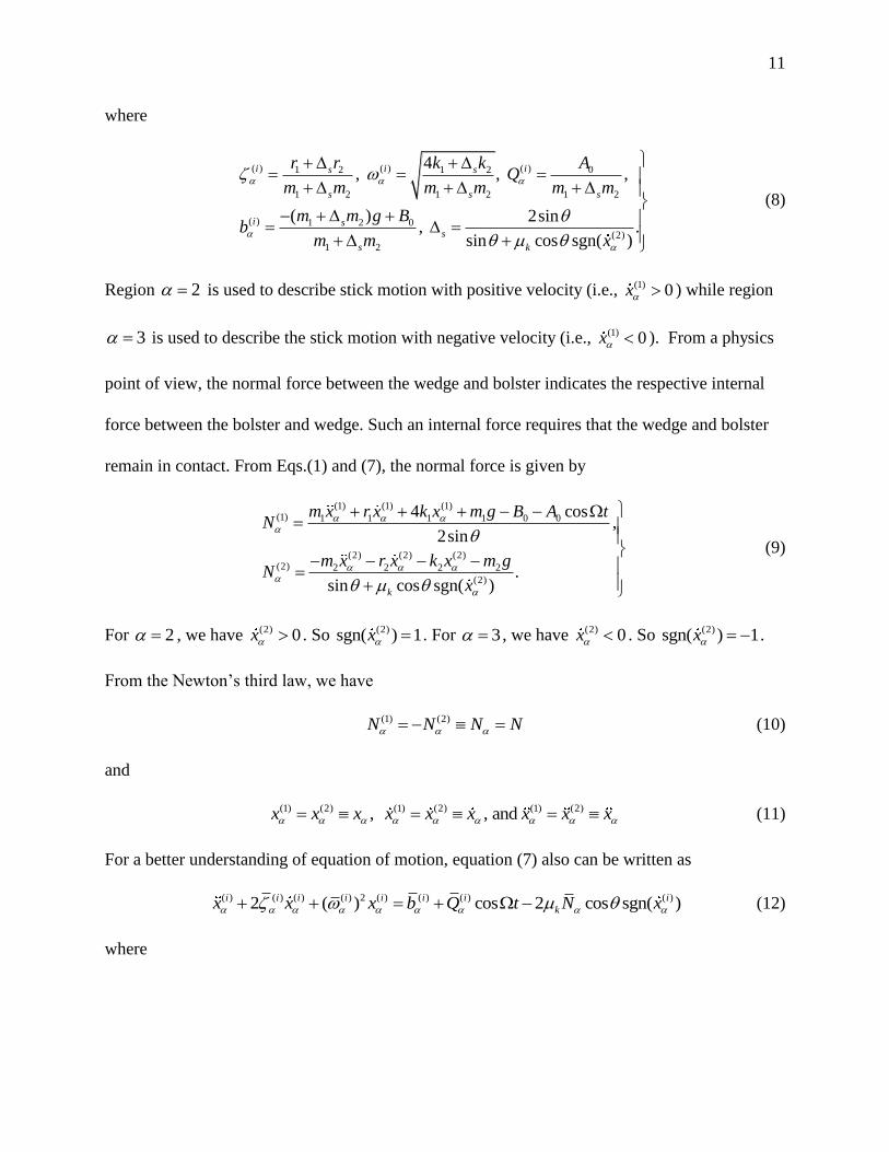
Region 2 is used to describe stick motion with positive velocity (i.e., (1) 0x ) while region
3 is used to describe the stick motion with negative velocity (i.e., (1) 0x ). From a physics
point of view, the normal force between the wedge and bolster indicates the respective internal
force between the bolster and wedge. Such an internal force requires that the wedge and bolster
remain in contact. From Eqs.(1) and (7), the normal force is given by
(1) (1) (1)(1) 1 1 1 1 0 0
(2) (2) (2)(2) 2 2 2 2
(2)
4 cos,
2sin
.sin cos sgn( )k
m x r x k x m g B A tN
m x r x k x m gN
x
(9)
For 2 , we have (2) 0x . So (2)sgn( ) 1x . For 3 , we have (2) 0x . So (2)sgn( ) 1x .
From the Newton’s third law, we have
(1) (2)N N N N (10)
and
(1) (2) (1) (2) (1) (2), , and x x x x x x x x x (11)
For a better understanding of equation of motion, equation (7) also can be written as
( ) ( ) ( ) ( ) 2 ( ) ( ) ( ) ( )2 ( ) cos 2 cos sgn( )i i i i i i i i
kx x x b Q t N x (12)
where

12
0 ( )k N t
(1)x
0 ( ) k N t
fF
Figure 2.3. Friction model varying with time.
( ) ( )1 2 1 2
1 2 1 2 1 2
( ) ( )0 1 2 0
1 2 1 2
2 4 2, ,
2 2 2
( 2 ), .
2 2
i i
i i
Nr r k kN
m m m m m m
A m m g BQ b
m m m m
(13)
The normal force N can be computed from Eqs. (9)–(11). Since the normal force between the
wedge and bolster may vary with time, the force of friction is also a function of time. To
illustrate this, the friction force in Eq.(5) is shown in Figure 2.3. In physics, the normal force is
actually the internal force that keeps the bolster and wedge together, the vanishing of stick
motion vanishing requires for 1,2i
( ) 0.iN N (14)
Consequently, the stick condition for the three oscillators is given for 1,2i and 2,3
( ) 0.iN N (15)
In the region of 1 , the bolster and wedge do not interfere with each other, so ( ) 0iN holds
always. Finally, if the friction force acting on the combined mass system is greater than or equal

13
to the resultant dynamic forces, then the bolster and wedges will become “stuck” against the side
wall. In other words, the wedge with bolster does not move.
2.2 Absolute Motions
The bolster and pair of wedges represent a discontinuous system because of their possible
impacts and the friction force acting on the wedges. Accordingly, the vector fields for each
oscillator are discontinuous. Consider the free-flight region described earlier as 1 . For
( {1,2}i,i and i i ), domain ( )
1
i in phase plane for free-flight motion is defined as
( ) ( ) ( ) ( ) ( )
1 1( , ) ( ( ), ), (0, )i i i i i
m mx x x x t t (16)
Since the bolster and wedge displacements are changing with time, ( )
1 ( )i
mx t describes the lower
bound for ( )
1
ix where mt is the impact time. The boundary ( )
1
i
of the domain ( )
1
i is defined as
( ) ( ) ( )
1 1( ) ( ) ( )
1 ( ) ( )
1
( ) 0( , )
( ), (0, )
i i i
mi i i
i i
m m
x x tx x
x x t t
(17)
which is a non-passable boundary or infinite flow barrier. In Figure 2.4, the shaded region is the
domains for the free-fright motion. The dash dot curve is the boundary ( )
1
i
, which is
instantaneous at time mt with the vertical dotted lines. In Figure 2.4(a), the domain and boundary
for the free-flight motion of the bolster is presented. The domain lies on the right side of the
boundary relative to the wedges. Since the wedges are below the bolster, the domain and
boundary for the free-flight motion of wedges are presented in Figure 2.4(b), and the domain lies
on the left side of the boundary relative to the bolster.

14
(a)
(1)x
(1)x
(1)
1
(1)
1
mt
Free Flight
(b)
(2)x
(2)x
(2)
1
(2)
1
mt
Free Flight
Figure 2.4. Free-flight domain and boundary: (a) bolster and (b) wedges.

15
Consider the regions ( 2,3 ) for stick motion when the bolster and wedges are sticking
together. The domains ( )
2
i and ( )
3
i in phase plane are for stick motion with frictional force. In
domain ( )
2
i , the velocity of the combined system is positive, so the frictional force acts in the
negative direction. However, in domain ( )
3
i , the friction force acts in the positive direction.
( ) ( ) ( )
2 2( ) ( ) ( )
2 ( )
( ) ( ) ( )
2 2( ) ( ) ( )
3 ( )
( , ), ( , ) ,
(0, )
( , ), ( , ) .
( ,0)
i i i
i i i
i
i i i
i i i
i
x x xx x
x
x x xx x
x
(18)
Herein ( )i
is defined as the closure of ( )i
( 1,2)i and ( 2,3) . The corresponding
separation boundaries ( )
23
i and ( )
32
i for the stick motion are defined as for positive and
negative displacement, respectively.
( ) ( ) ( )
( ) ( ) ( ) ( ) ( )
23 2 3 ( ) ( )
23
( ) ( ) ( )
( ) ( ) ( ) ( ) ( )
32 2 3 ( ) ( )
32
0, 0( , ) ,
0
0, 0( , ) .
0
i i i
i i i i i
i i
i i i
i i i i i
i i
x x xx x
x
x x xx x
x
(19)
In Figure 2.5, the hatched regions are for ( )
2
i and ( )
3
i ( 1,2i ), define the region of stick
motion with positive and negative velocity, respectively. Since the bolster wall is considered as
the fixed inertial reference frame, the velocity boundary separating ( )
2
i and ( )
3
i is at ( ) 0ix
and is represented by the dotted line. The vertical arrows drawn across the boundary show the
direction of the motion flow. For 1i , the domains for the bolster are presented in Figure 2.5(a).
For 2i , the domain for the wedges are presented in Figure 2.5(b). For the stick motion, the
bolster and wedges are together to form a new oscillator. Thus, the domains and boundary are
same.

16
(a)
(1)
2x
(1)
2
( )ix
(1)
3
(1)
32(1)
23
(b)
(2)
2
(2)x
(2)
3
(2)
32(2)
23
(2)x
Figure 2.5. Phase plane domains and boundaries for stick motion: (a) bolster and (b).
wedges.
17
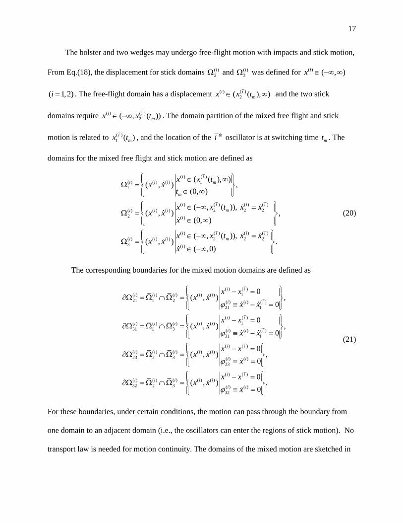
The bolster and two wedges may undergo free-flight motion with impacts and stick motion,
From Eq.(18), the displacement for stick domains ( )
2
i and ( )
3
i was defined for ( ) ( , )ix
( 1,2)i . The free-flight domain has a displacement ( ) ( )
2( ( ), )i i
mx x t and the two stick
domains require ( ) ( )
2( , ( ))i i
mx x t . The domain partition of the mixed free flight and stick
motion is related to ( )
1 ( )i
mx t , and the location of the thi oscillator is at switching time mt . The
domains for the mixed free flight and stick motion are defined as
( ) ( )
( ) ( ) ( ) 1
1
( ) ( ) ( ) ( )
2 2 2( ) ( ) ( )
2 ( )
( ) ( ) ( ) ( )
2 2 2( ) ( ) ( )
3 ( )
( ( ), )( , ) ,
(0, )
( , ( )), ( , ) ,
(0, )
( , ( )), ( , )
( ,0)
i i
i i i m
m
i i i i
mi i i
i
i i i i
mi i i
i
x x tx x
t
x x t x xx x
x
x x t x xx x
x
.
(20)
The corresponding boundaries for the mixed motion domains are defined as
( ) ( )
1( ) ( ) ( ) ( ) ( )
21 1 2 ( ) ( ) ( )
21 1
( ) ( )
1( ) ( ) ( ) ( ) ( )
31 1 3 ( ) ( ) ( )
31 1
( ) ( )
( ) ( ) ( ) ( ) ( )
23 2 3 (
23
0( , ) ,
0
0( , ) ,
0
0( , )
i i
i i i i i
i i i
i i
i i i i i
i i i
i i
i i i i i
i
x xx x
x x
x xx x
x x
x xx x
) ( )
( ) ( )
( ) ( ) ( ) ( ) ( )
32 2 3 ( ) ( )
32
,0
0( , ) .
0
i
i i
i i i i i
i i
x
x xx x
x
(21)
For these boundaries, under certain conditions, the motion can pass through the boundary from
one domain to an adjacent domain (i.e., the oscillators can enter the regions of stick motion). No
transport law is needed for motion continuity. The domains of the mixed motion are sketched in
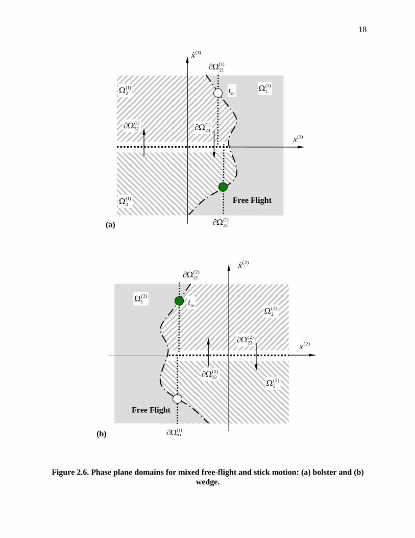
18
(a)
(1)x
(1)
2
(1)
3
(1)
32
(1)
21
(1)x
(1)
31
(1)
23
(1)
1mt
Free Flight
(b)
( )
2
i
( )
3
i
( )
32
i
(2)
21
(2)x
( )
31
i
(2)
23
(2)
1mt
Free Flight
(2)
2
(2)x
(2)
3
(2)
32
Figure 2.6. Phase plane domains for mixed free-flight and stick motion: (a) bolster and (b)
wedge.

19
Figure 2.6(a) and (b) for the bolster and wedges, respectively. The domain ( )
1
i ( 1,2i ) for the
flight motion of the bolster is represented by the shaded region, and two domains for stick
motions are represented by the two hatched regions, labeled as ( )
2
i and ( )
3
i ( 1,2i ). Again,
the dotted line at ( ) 0ix ( 1,2i ) represents the velocity boundary for wedges’ friction with side
walls. The boundaries for the onset and vanishing of stick motion are sketched by the dash-dot
line, and the switching times mt mark the locations for the appearance and disappearance of stick
motions. The hollow and solid circular symbols represent the starting and ending of stick motion,
respectively.
In the absolute reference frame, the following vectors are introduced as
( ) ( ) ( ) ( ) ( )
( ) ( ) ( ) ( ) ( )
( , ) ( , ) ,
( , ) ( , ) .
i i i T i i T
i i i T i i T
x x x y
x F y F
x
F (22)
With Eq.(22), equations of motion for free-fright motion in Eq.(1) and stick motion in Eq.(7) can
be represented for as
( ) ( ) ( )( , ) for 1,2,3 and 1,2i i i t i x F x (23)
where
( ) ( ) ( ) ( ) 2 ( ) ( ) ( )2 ( ) cosi i i i i i iF x x b Q t (24)
and the superscript “i” represents the ith mass and the subscript “ ” represents the -domain.
For the boundary 1 , the flow cannot pass through the boundary, thus the impact chatter will
occurs. For the boundary 1 ( 2 3, ), the flow will pass through the boundary from domain
1 to domain 2 or from domain 3 to domain 1 . On the boundary 23 , there is sliding
motion.

20
( ) ( ) ( )
0 0 0( , ) for , 2,3 and 1,2i i i t i x F x (25)
where
( )
0
( )
0 23
0 for stick
[ 2 cos ,2 cos ] on boundary
i
i
k k
F
F N N
(26)
2.3 Relative motion
Because the boundaries that separate free-flight and stick motion vary with time, the
analytical conditions for the motion mechanisms of bolster and wedge interaction with a moving
boundary is be difficult to be obtained. Hence, two relative variables are introduced herein as
( ) ( ) ( ) ( ) ( ) ( ) ( ) and .i i i i i i iz x x v z x x (27)
From the foregoing equation, the equations of motion are for , 1,2i i ( i i ) and 1,2,3
( ) ( ) ( ) ( ) 2 ( ) ( ) ( ) ( ) ( ) ( ) ( ) 2 ( )
( ) ( ) ( ) ( ) 2 ( ) ( ) ( )
2 ( ) cos 2 ( ) ,
2 ( ) cos .
i i i i i i i i i i i i
i i i i i i i
z z z b Q t x x x
x x x b Q t
(28)
In a similar fashion, two more vectors are introduced as follows.
( ) ( ) ( ) ( ) ( )
( ) ( ) ( ) ( ) ( )
( , ) ( , )
( , ) ( , )
i i i T i i T
i i i T i i T
z z z v
z g v g
z
g (29)
From Eqs.(28) and (29), the equations of motion become for 1,2i and 1,2,3
( ) ( ) ( ) ( )
( ) ( ) ( )
( , , )
( , )
i i i i
i i i
t
t
z g z x
x F x (30)
where
( ) ( ) ( ) ( ) 2 ( ) ( ) ( )
( ) ( ) ( ) ( ) 2 ( )
2 ( ) cos
2 ( ) .
i i i i i i i
i i i i i
g z z b Q t
x x x
(31)
Because the stick motion requires the relative motion to vanish between the wedge and bolsters,

21
the domains ( )
2
i and ( )
3
i become two points in relative phase space. In the relative frame, the
sub-domains in Eq.(17) can be expressed by
( ) ( ) ( ) ( ) ( )
1
( ) ( ) ( ) ( ) ( )
2
( ) ( ) ( ) ( ) ( )
3
( , ) (0, ), ( , ) ,
( , ) 0, 0 ,
( , ) 0, 0 .
i i i i i
i i i i i
i i i i i
z z z z
z z z z
z z z z
(32)
In the relative frame, the impacting chatter boundaries in Eq.(14) become
( ) ( ) ( ) ( ) ( )
1 1( , ) 0i i i i iz z z (33)
Through their subsets, such boundary sets become
( ) ( ) ( )
1 1 1
i i i
(34)
where
( ) ( ) ( ) ( ) ( ) ( )
1 1
( ) ( ) ( ) ( ) ( ) ( )
1 1
( , ) 0, (0, ) ,
( , ) 0, ( ,0) .
i i i i i i
i i i i i i
z z z z
z z z z
(35)
The stick boundary become one points, which is expressed by
( ) ( ) ( ) ( ) ( ) ( )
32 23
( ) ( ) ( ) ( ) ( ) ( )
23 23
( , ) 0, 0 ,
( , ) 0, 0 .
i i i i i i
i i i i i i
z z z z
z z z z
(36)
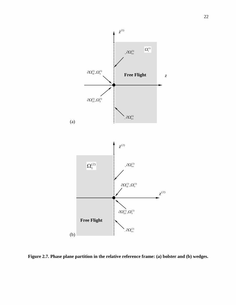
The boundaries in the relative frame are independent of time. The phase partitions in relative
phase space for the bolster and wedges are sketched in Figure 2.7(a) and (b), respectively. The
stick boundaries and domains are presented by the two large dots.
22
(a)
(1)
1
(1) (1)
32 3,
(1) (1)
23 3,
(1)z
(1)z
(1)
1
(1)
1
Free Flight
(b)
(2)
1
(2) (2)
32 3,
(2) (2)
23 3,
(2)z
(2)z
(2)
1
(2)
1
Free Flight
Figure 2.7. Phase plane partition in the relative reference frame: (a) bolster and (b) wedges.

23
CHAPTER III
MOTION MECHANISMS
The domains and boundaries of the different types of motion were introduced in Chapter
2. This chapter considers how motion may interact with the boundary separating two different
domains. In other words, the necessary and sufficient conditions for passable boundaries,
grazing, and stick motions will be developed to give analytical conditions for motion
mechanisms. Based on discontinuous dynamical system theory, the equations of motion in the
relative and absolute reference frame will be utilized to obtain such conditions. To help
understand these analytical conditions, physical explanations of such analytical conditions will be
presented.
3.1 Stuck and Sliding Conditions
To investigate the motion mechanism of the discontinuous suspension model, both the
absolute and relative coordinate systems will be utilized. For the stick motion (i.e., bolster and
wedge already joined) and the corresponding velocity boundary, the absolute reference frame will
be used. For free flight chatters with possible stick motion, the relative coordinate system will be
adopted. To develop analytical conditions for motion switching at the boundary ( )i
, from Luo
(2009) and (2012), the following G-functions are introduced as
( )
(0, ) ( ) T ( ) ( ) (0) ( )( , ) ( , ) ( , ) ,i
i i i i
m m mG t t t
x n F x F x (37)
( )
( )
(1, ) ( ) T ( ) ( ) (0) ( )
T ( ) ( ) (0) ( )
( , ) 2 ( , ) ( , )
+ ( , ) ( , ) ,
i
i
i i i i
m m m
i i i
m m
G t D t t
D t D t
x n F x F x
n F x F x (38)
where ( ) ( ) ( )D t x x . If the normal vector ( )i
n is a unit vector, the G-function in

24
Eq.(37) gives the normal component of the difference between the vector field within a domain
and the vector field on a boundary. The time-change rate of the G-function is given in Eq.(38),
which is the first order G-function. The switching time mt represents the time for motion on the
boundary, and 0m mt t reflects the responses in the domains rather than on the boundary.
The vector field ( ) ( )( , )i i
mt F x is for a flow of the ith oscillator in domain ( )i
, and the vector field
(0) ( )( , )i t F x is for a flow on the boundary ( )i
. The normal vector ( )n i
of the boundary ( )i
is computed by
( )
T( ) ( )
( )
( ) ( ),i
i i
i
i ix y
n (39)
where T
,x y is the Hamilton operator. Because ( )
T (0) ( )( , ) 0i
i
mt
n F x , its total
derivative gives
( ) ( )
T (0) ( ) T (0) ( )( , ) ( , ) 0.i i
i i
m mD t D t
n F x n F x (40)
If the boundary ( )i
is a line independent of time t, ( )
T 0iDn . Therefore, equation (40)
becomes
( )
T (0) ( )( , ) 0.i
i
mD t
n F x (41)
Notice that (0) T( , ) (0,0)t F x on the boundary
( )i
. Taking the time change rate of the
T
( ) ( )( ) ( ) ( ) ( ) ( ) ( ) ( ) ( ) ( , )
, ( , ), ( , ) ( , ) .i i
i i i i i i i i
m
F tD t F t F t F t
t
xF x x x x (42)
Further, equations (37) and (38) reduce to
25
( )
( )
(0, ) ( ) T ( ) ( ) ( ) ( )
( ) ( )(1, ) ( ) T ( ) ( ) ( ) ( ) ( ) ( )
( , ) ( , ) ( , ), {2,3}
( , )( , ) ( , ) ( , ) ( , .
i
i
i i i i i
m m m
i ii i i i i i i
m m
G t t F t
F tG t D t F t t
t
x n F x x
xx n F x x F x
(43)
To investigate the stick motions in domains ( )i
( 2,3 ), the condition for a flow to pass
through the velocity boundary of ( ) ( )
23 0i ix and ( ) ( )
32 0i ix in Eq.(19) is very important.
From Luo (2009) and (2012), the passable motion to the boundary ( )i
is guaranteed by
( ) ( )
(0, ) ( ) (0, ) ( )
T ( ) ( ) T ( ) ( )
( ) ( , ) ( , )
[ ( , )] [ ( , )] 0.i i
i i
m m m m m
i i i i
m m m m
L t G t G t
t t
x x
n F x n F x (44)
In other words, the conditions for passable motion from domain ( )i
into ( )i
and vice versa
can be expressed as
( )
( )
( )
(0, ) ( ) T ( ) ( )
( ) ( )
(0, ) ( ) T ( ) ( )
(0, ) ( ) T ( ) ( )
(0
( 1) ( , ) ( 1) ( , ) 0
from ( 1) ( , ) ( 1) ( , ) 0
( 1) ( , ) ( 1) ( , ) 0
( 1)
i
i
i
i i i
m m m mi i
i i i
m m m m
i i i
m m m m
G t t
G t t
G t t
G
x n F x
x n F x
x n F x
( )
( ) ( )
, ) ( ) T ( ) ( )from .
( , ) ( 1) ( , ) 0i
i i
i i i
m m m mt t
x n F x
(45)
or more concisely as
(0, ) ( ) (0, ) ( )
( ) ( ) ( ) ( )
( ) ( , ) ( , )
( , ) ( , ) 0.
i i
m m m m m
i i i i
m m m m
L t G t G t
F t F t
x x
x x (46)
From Eq.(19) and (35), the normal vector ( )n i
to the boundary ( )i
for , {2,3}, is
given as
( ) ( )23 32
T(0,1) .i i
n n (47)
With Eq.(45) or (47), the passable conditions for , {2,3}, become
26
(a)
(1)
2
(1)x
(1)
3
(1)
32(1)
23
(1)y
32n
(1)
3 ( , )tF x
(0,3) (1)( , )m mG t x
(0,2) (1)( , )m mG t x (1)
2 ( , )tF x
( , )m tx
(b)
(1)
2
(1)x
(1)
3
(1)
32 (1)
23
(1)y
23n
(1)
3 ( , )tF x (0,3) (1)( , )m mG t x
(0,2) (1)( , )m mG t x (1)
2 ( , )tF x
( , )m tx
Figure 3.1. Passable flow illustration on (a) (1)
32 and (b) (1)
23 .

27
(0,2) ( ) ( ) ( )
2 ( ) ( )
2 3(0,3) ( ) ( ) ( )
3
(0,3) ( ) ( ) ( )
3 ( ) ( )
3 2(0,2) ( ) ( ) ( )
2
( , ) ( , ) 0from ,
( , ) ( , ) 0
( , ) ( , ) 0from .
( , ) ( , ) 0
i i i
m m m m i i
i i i
m m m m
i i i
m m m m i i
i i i
m m m m
G t F t
G t F t
G t F t
G t F t
x x
x x
x x
x x
(48)
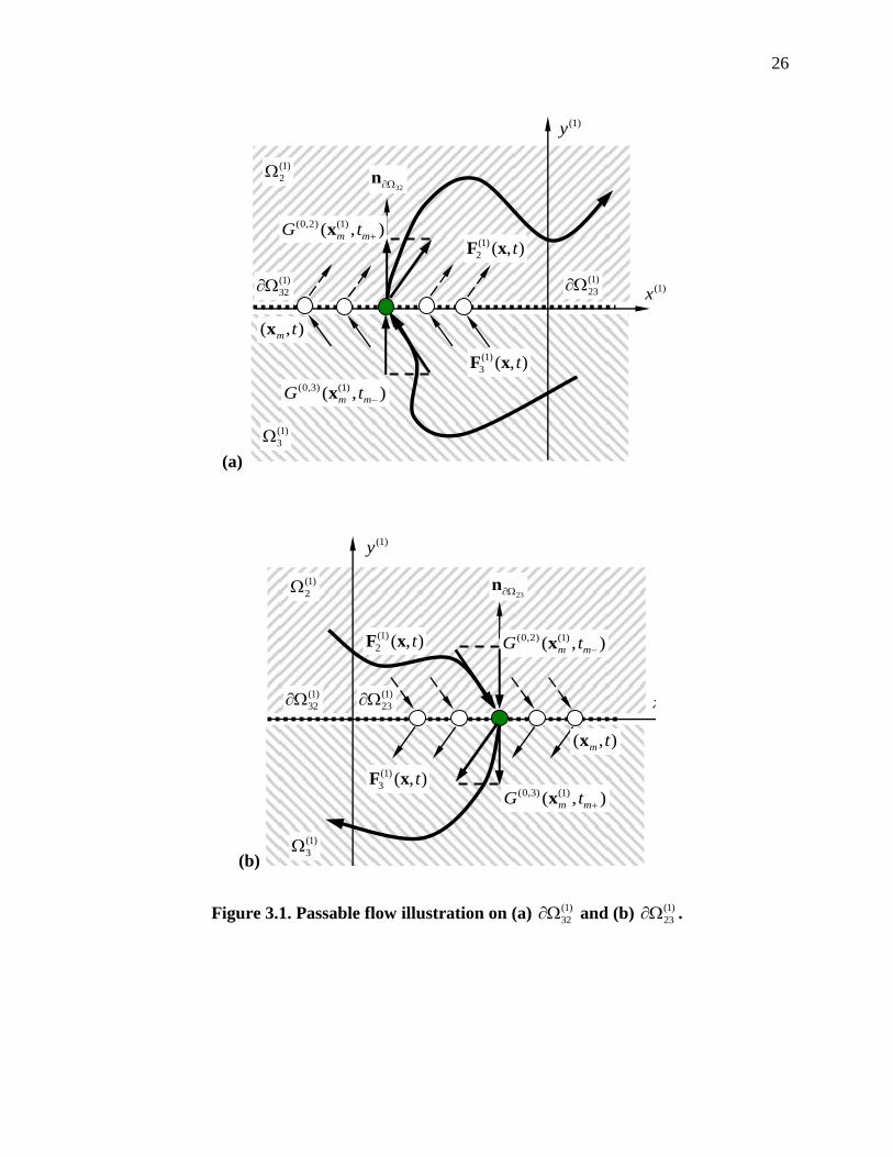
The aforementioned conditions are illustrated through the absolute frame as shown in Figure 3.1.
The solid grey curve represents the motion flow as it approaches and then passes through the
boundary at ( , )m mx t . The dashed and solid vectors labeled ( )
2 ( , )i tF x and ( )
3 ( , )i tF x illustrate the
vector fields in the domains 2 and 3 , respectively. In Figure 3.1(a), the conditions
(0,2) ( )( , )i
m mG t x and (0,3) ( )( , )i
m mG t x are both drawn in the positive direction along the normal
vector ( )i
n , thus reflecting that the motion passes the boundary ( )
32
i and enters ( )
2
i . Further,
for 1i and 2 , the conditions in Eq.(48) are same because oscillators 1 and 2 are combined
together. Thus, the analytical condition is
(1) (1) (1) (1) (1) (1)
2 3 3 2( , ) 0 and ( , ) 0 from .m m m mF t F t x x (49)
In a similar manner, Figure 3.1(b) can be discussed.
From [Luo, 2009, 2012], the stuck motion on ( )i
is guaranteed by
( ) ( )
(0, ) ( ) (0, ) ( )
T ( ) ( ) T ( ) ( )
( ) ( , ) ( , )
[ ( , )] [ ( , )] 0.i i
i i
m m m m m
i i i i
m m m m
L t G t G t
t t
x x
n F x n F x (50)
Here the stuck condition requires a negative cross product. For the boundary ( )i
with
( )
T ( )i
i
n the necessary and sufficient conditions for non-passable motion to the boundary
(i.e., stuck motion) are expressed as
28
( )
( )
(0, ) ( ) T ( ) ( )
(0, ) ( ) T ( ) ( )
( 1) ( , ) ( 1) ( , ) 0,
( 1) ( , ) ( 1) ( , ) 0.
i
i
i i i
m m m m
i i i
m m m m
G t t
G t t
x n F x
x n F x (51)
With Eq.(47), the stuck conditions in Eq.(51) are simplified for , {2,3}, as
(0,2) ( ) ( ) ( )
2 ( )
23(0,3) ( ) ( ) ( )
3
( , ) ( , ) 0,on .
( , ) ( , ) 0,
i i i
m m m m i
i i i
m m m m
G t F t
G t F t
x x
x x (52)
The foregoing equation means that for stuck motion to occur for 1i , the force per unit mass (or
acceleration) on the boundary (1)
23 and (1)
32 must be negative just inside (1)
2 and positive just
inside (1)
3 . The requirement to keep the stuck motion is given by
(1) (1) (1) (1)
2 3( , ) 0 and ( , ) 0.m m m mF t F t x x (53)
Since the oscillator 1 and oscillator 2 with stick are together. So the oscillator has the same
conditions in Eq,(53). If two coming flows in phase plane reach the velocity boundary (1)
23
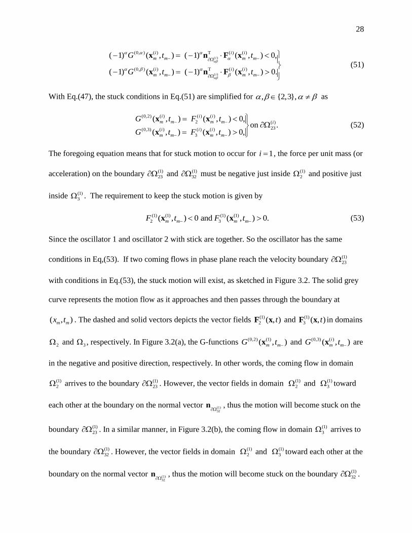
with conditions in Eq.(53), the stuck motion will exist, as sketched in Figure 3.2. The solid grey
curve represents the motion flow as it approaches and then passes through the boundary at
( , )m mx t . The dashed and solid vectors depicts the vector fields (1)
2 ( , )tF x and (1)
3 ( , )tF x in domains
2 and 3 , respectively. In Figure 3.2(a), the G-functions (0,2) (1)( , )m mG t x and (0,3) ( )( , )i
m mG t x are
in the negative and positive direction, respectively. In other words, the coming flow in domain
(1)
2 arrives to the boundary (1)
23 . However, the vector fields in domain (1)
2 and (1)
3 toward
each other at the boundary on the normal vector (1)32
n , thus the motion will become stuck on the
boundary (1)
23 . In a similar manner, in Figure 3.2(b), the coming flow in domain (1)
3 arrives to
the boundary (1)
32 . However, the vector fields in domain (1)
2 and (1)
3 toward each other at the
boundary on the normal vector (1)32
n , thus the motion will become stuck on the boundary (1)
32 .
29
(a)
(1)
2
(1)x
(1)
3
(1)
32 (1)
23
(1)y
32n
(1)
3 ( , )tF x (0,3) (1)( , )m mG t x
(0,2) (1)( , )m mG t x (1)
2 ( , )tF x
( , )m tx
(b)
(1)
2
(1)x
(1)
3
(1)
32 (1)
23
(1)y
23n
(1)
2 ( , )tF x
(0,3) (1)( , )m mG t x
(0,2) (1)( , )m mG t x
( , )m tx
Figure 3.2. Stuck motion on (a) (1)
32 and (b) (1)
23 .
For stuck motion vanishing, the wedge combined with the bolster will start to move on the
both side walls. The G-function (0, ) ( )( , )i
m mG tx will equal zero for stuck vanishing and moving to

30
the domain ( )i
, the time change rate of the G-function (i.e., (1,2) ( )( , )i
m mG t x ) must be considered
to guarantee vanishing of the stuck motion. From Luo (2009) and (2012), the analytical
conditions are
( )32
( )32
( )32
(0,3) ( ) T ( ) ( )
3
(0,2) ( ) T ( ) ( ) ( ) ( )
2 32 2
(1,2) ( ) T ( ) ( )
2
( , ) ( , ) 0
( , ) ( , ) 0 from
( , ) ( , ) 0
i
i
i
i i i
m m m m
i i i i i
m m m m
i i i
m m m m
G t t
G t t
G t D t
x n F x
x n F x
x n F x
(54)
( )23
( )23
( )23
(0,2) ( ) T ( ) ( )
2
(0,3) ( ) T ( ) ( ) ( ) ( )
3 23 3
(1,3) ( ) T ( ) ( )
3
( , ) ( , ) 0
( , ) ( , ) 0 from .
( , ) ( , ) 0
i
i
i
i i i
m m m m
i i i i i
m m m m
i i i
m m m m
G t t
G t t
G t D t
x n F x
x n F x
x n F x
(55)
From Eq.(39), (1, ) ( )( , )i
iG t
x is given by the following equation
(1, ) ( ) ( ) ( ) ( ) 2 ( ) ( )( , ) 2 ( ) sin .i i i i i iG t x x Q t
x (56)
From a physical point of view, equation (56) describes the absolute jerk, namely
( ) ( ) ( ) ( ) 2 ( ) ( )( ) 2 ( ) sin .i i i i i iJ t x x Q t (57)
Consider the stuck motion on (1)
32 for 1i . If (0,2) ( )
2( , ) 0i
mG t x and (1,2) ( )( , ) 0i
m mG t x ,
then for mt t , (0,2) ( )
2( , ) 0i
mG t x will be true. The analytical conditions for the vanishing of
stuck motion are further simplified and given below for , {2,3}, .
(0,3) ( ) ( ) ( )
3
(0,2) ( ) ( ) ( ) ( ) ( )
2 32 2
(1,2) ( )
( , ) ( , ) 0
( , ) ( , ) 0 from
( , ) 0
i i i
m m m m
i i i i i
m m m m
i
m m
G t F t
G t F t
G t
x x
x x
x
(58)
(0,2) ( ) ( ) ( )
2
(0,3) ( ) ( ) ( ) ( ) ( )
3 32 3
(1,3) ( )
( , ) ( , ) 0
( , ) ( , ) 0 from
( , ) 0
i i i
m m m m
i i i i i
m m m m
i
m m
G t F t
G t F t
G t
x x
x x
x
(59)

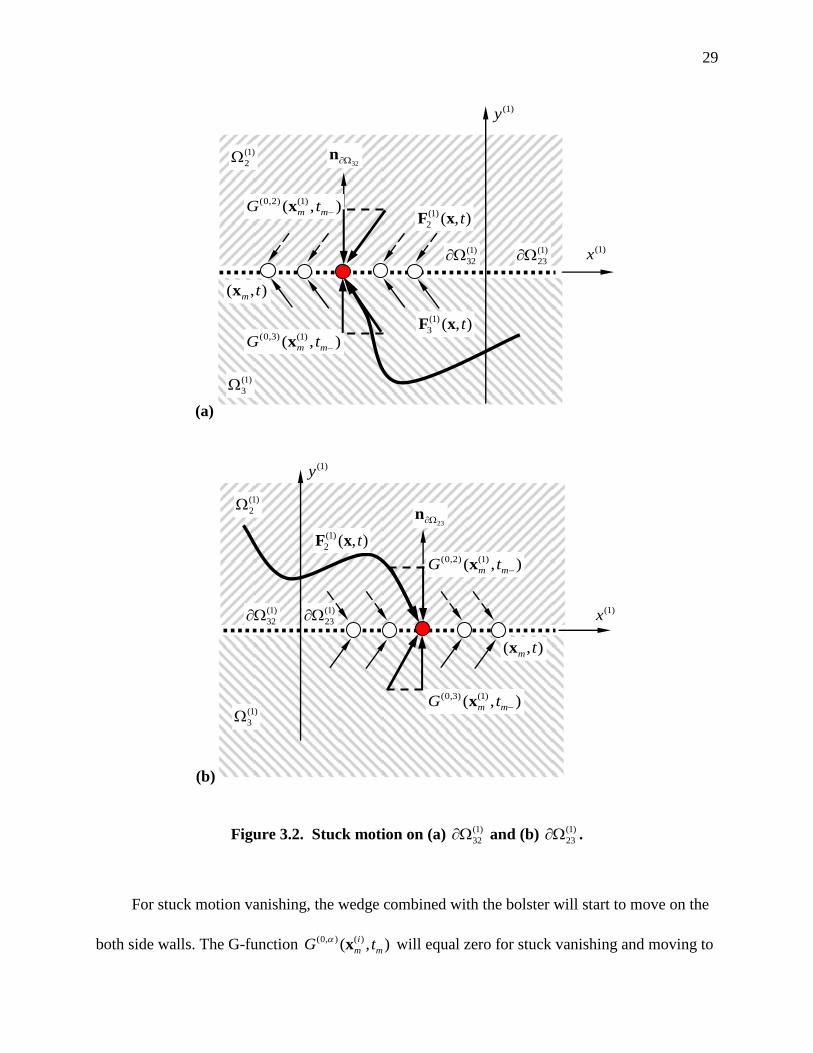
31
In Figure 3.3, a leaving flow from the boundary to domain is presented when the vanishing of
stuck motion occurs. The solid red circle represents the static position where the bolster and
wedges are stuck against the wall. The solid grey curve shows the motion leaving the stuck
position. The dashed and solid vectors labeled ( )
2 ( , )i tF x and ( )
3 ( , )i tF x illustrate the vector fields
in the domains 2 and 3 , respectively. In Figure 3.3(a), the motion is from the boundary (1)
23
to domain (1)
2 . Due to (1) (1)
2 ( , ) 0m mF t x with (1,2) (1)( , ) 0m mG t x , then (1) (1)
2 ( , ) 0m mF t x for
0 . In a similar manner, Figure 3.3(b), a leaving motion is from the boundary (1)
32 to domain
(1)
3 because (1) (1)
3 ( , ) 0m mF t x with (1,2) (1)( , ) 0m mG t x , then (1) (1)
3 ( , ) 0m mF t x for 0 .
From Eq.(58) for 1i , when (1) (1)
2 ( , ) 0m mF t x , we have (1,2) (1)( , ) 0m mG t x . As a result, at
the next moment (1) (1)
2 ( , ) 0m mF t x would be negative and the stuck conditions of Eq.(49) would
be satisfied. This phenomena is called the grazing of stuck, and the conditions are described as
(0,3) ( ) ( ) ( )
3
(0,2) ( ) ( ) ( ) ( )
2 23
(1,2) ( )
(0,2) ( ) ( ) ( )
2
(0,3) ( ) ( ) ( )
3
(1,3) ( )
( , ) ( , ) 0
( , ) ( , ) 0 on
( , ) 0
( , ) ( , ) 0
( , ) ( , ) 0
( , ) 0
i i i
m m m m
i i i i
m m m m
i
m m
i i i
m m m m
i i i
m m m m
i
m m
G t F t
G t F t
G t
G t F t
G t F t
G t
x x
x x
x
x x
x x
x
( )
32on i
(60)
Consider the grazing of the stuck motion on the boundary 32 for 1i , then (1) (1)
3 ( , ) 0m mF t x
and (1) (1)
2 ( , ) 0m mF t x . However, due to (1,2) (1)( , ) 0m mG t x , at the next instance, we have
(1) (1)
2 ( , ) 0m mF t x and the stuck motion conditions of Eq.(53) will be satisfied.
32
(a)
(1)
2
(1)x
(1)
3
(1)
32(1)
23
(1)y
23n
(1)
3 ( , )tF x (0,3) (1)( , )m mG t x
(0,2) (1)( , )m mG t x (1)
2 ( , )tF x
( , )m tx
(b)
(1)
2
(1)x
(1)
3
(1)
32 (1)
23
(1)y
23n
(1)
3 ( , )tF x (0,3) (1)( , )m mG t x
(0,2) (1)( , )m mG t x ( )
2 ( , )i tF x
( , )m tx
Figure 3.3. Vanishing of stuck motion: (a) from ( )
32
i to ( )
2
i and (b) form ( )
23
i to ( )
3
i .

33
3.2 Free-flight and stick motions
To discuss the free-flight and stick motions, the relative coordinate system is adopted. From
Eq.(30), the relative coordinate systems is utilized to define the following two functions for
, {2,3}, .
( )
(0, ) ( ) ( ) ( ) ( ) ( ) (0) ( ) ( )( , , ) ( , , ) ( , , ) ,i
i i T i i i i i
m m mG t t t
z x n g z x g z x (61)
( )
( )
(1, ) ( ) ( ) ( ) ( ) ( ) (0) ( ) ( )
( ) ( ) ( ) (0) ( ) ( )
( , , ) 2 [ ( , , ) ( , , )]
+ [ ( , , ) ( , , )].
i
i
i i T i i i i i
m m m
T i i i i i
m m
G t D t t
D t D t
z x n g z x g z x
n g z x g z x (62)
For the free-flight impact chatter, from Eq.(33) the normal vector ( )1i
n to the boundary ( )
1
i
is
( )1
T( ) ( )
( ) T
( ) ( ), (1,0) .i
i i
i
i iz z
n (63)
Therefore, equations (61) and (62) give
( )1
( )1
(0,1) ( ) ( ) T ( ) ( ) ( ) ( )
1 1 1 1 1 1
(1,1) ( ) ( ) T ( ) ( ) ( ) ( ) ( ) ( )
1 1 1 1 1 1 1 1
( , , ) ( , , ) ,
( , , ) ( , , ) ( , , ).
i
i
i i i i i i
m m
i i i i i i i i
m m m
G t t v
G t D t g t
z x n g z x
z x n g z x z x (64)
From Luo (2009) and (2012), the analytical conditions for grazing motions on the impact
boundary are
( ) ( ) ( ) ( ) ( )
1 1 1 1 1( ) 0 and ( 1) ( , , ) 0 on i i i i i i
m mv t g t z x (65)
For 1i , the bolster and wedges just contact, the conditions in Eq.(62) give (1)
1 ( ) 0mv t and
(1) (1) (2)
1 1 2( , , ) 0mg t z x . For mt t , the relative velocity (1)
1 ( ) 0mv t because (1)
1 0g . With
negative relative velocity, the relative displacement (1)
1 ( ) 0mz t will be satisfied. In other
words, the bolster remains in (1)
1 . Such a phenomenon is called grazing motion to the boundary
(1)
1 , as shown in Figure 3.4. The black curve in (1)
1 approaches the boundary (1)
1 but turns

34
away without interaction to the boundary.
From Luo (2009) and (2012), the passable motion to the boundary ( )i
is guaranteed by
( ) ( )
(0, ) ( ) ( ) (0, ) ( ) ( )
T ( ) ( ) ( ) T ( ) ( ) ( )
( ) ( , , ) ( , , )
[ ( , , )] [ ( , , )] 0.i i
i i i i
m m m
i i i i i i
m m
L t G t G t
t t
z x z x
n g z x n g z x (66)
Passable motion to the boundary ( )i
means the onset of stick motion (i.e., the bolster and
wedges move as one). From Luo (2009) and (2012), the conditions for stick motion can also be
written as
( )
( )
( )
(0, ) ( ) ( ) T ( ) ( ) ( )
( )
(0, ) ( ) ( ) T ( ) ( ) ( )
(0, ) ( ) ( )
( 1) ( , , ) ( 1) ( , , ) 0,
for ,( 1) ( , , ) ( 1) ( , , ) 0
( 1) ( , , ) ( 1)
i
i
i
i i i i i i i
m mi
i i i i i i i
m m
i i i i
m
G t t
G t t
G t
z x n g z x
nz x n g z x
z x n ( )
( )
( )
T ( ) ( ) ( )
( )
(0, ) ( ) ( ) T ( ) ( ) ( )
( , , ) 0,
for .( 1) ( , , ) ( 1) ( , , ) 0
i
i
i
i i i
mi
i i i i i i i
m m
t
G t t
g z x
nz x n g z x
(67)
(1)
1
( ) ( )
2 3,i i
(1)v
( )iz
(1)
1
1n
(1) (1) (2)
1 1 1( , , )mg t z x
(1)
1( , )mtz
(1) (1) (2)
1 1 1( , x , )mg t z
Figure 3.4. Free-flight motion grazing at (1)
1 .

35
With Eq.(36), the normal vector ( )i
n to the boundary ( )i
for , {1,2,3}, is
( ) ( )21 31
T(0,1) .i i
n n (68)
The G-function in Eq,(67) is
( )
( )
(0, ) ( ) ( ) T ( ) ( ) ( ) ( ) ( ) ( )
(1, ) ( ) ( ) T ( ) ( ) ( )
( ) (( ) ( ) ( ) ( ) ( ) ( )
( , , ) ( , , ) ( , , ), [2,3]
( , , ) ( , , )
(( , , ) ( , , )
i
i
i i i i i i i i
m m m
i i i i i
m m
ii i i i i i
G t t g t
G t D t
gg t t
z x n g z x z x
z x n g z x
zz x g z x
) ( ), , ).
i i t
t
x
(70)
For motion entering domain 3 from 1 , the passable conditions in Eq.(67) is
(0,1) ( ) ( ) ( ) ( ) ( )
1 1 1 1 1 ( ) ( )
1 3(0,3) ( ) ( ) ( ) ( ) ( )
3 3 3 3 3
( 1) ( , , ) ( 1) ( , , ) 0, for .
( 1) ( , , ) ( 1) ( , , ) 0
i i i i i i i
m m i i
i i i i i i i
m m
G t g t
G t g t
z x z x
z x z x (71)
The conditions for motion from domain ( )
1
i to ( )
2
i are given by
(0,1) ( ) ( ) ( ) ( ) ( )
1 1 1 1 1 ( ) ( )
1 2(0,2) ( ) ( ) ( ) ( ) ( )
2 2 2 2 2
( 1) ( , , ) ( 1) ( , , ) 0,for .
( 1) ( , , ) ( 1) ( , , ) 0
i i i i i i i
m m i i
i i i i i i i
m m
G t g t
G t g t
z x z x
z x z x (72)
The foregoing equation gives the analytical conditions for stick motion of the bolster and edges.
The relative force per unit mass (or relative acceleration) in (1) (1)
2 1and must be negative on
the boundary (1)
21 . Also, the relative acceleration in (1) (1)
3 1and must be negative on the
boundary (1)
31 . The stick conditions of Eq.(71) gives
(1) (1) (2) (1) (1) (2)
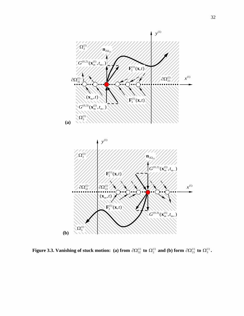
1 1 1 3 1 1g ( , , ) 0 and g ( , , ) 0.m mt t z x z x (73)
From Eq.(36), the stick motion requires that the relative displacement and velocity equal zero
(i.e., (1)
1 0z and (1)
1 0z ). The conditions for stick motion are depicted in the absolute
coordinate system in Figure 3.5.
36
(1)
2
( )
3
i
(1)
21
(1)x
(1)
13
(1)
1
mt31n
(0,3) (1) (1)
3 3( , , )mG t z x
(0,1) (1) (1)
1 1( , , )mG t z x
(1)y
Figure 3.5. Stick motion on (1)
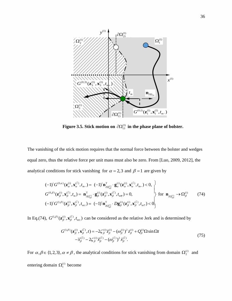
13 in the phase plane of bolster.
The vanishing of the stick motion requires that the normal force between the bolster and wedges
equal zero, thus the relative force per unit mass must also be zero. From [Luo, 2009, 2012], the
analytical conditions for stick vanishing for 2,3 and 1 are given by
( )
( )
( )
(0, ) ( ) ( ) T ( ) ( ) ( )
(0, ) ( ) ( ) T ( ) ( ) ( )
(1, ) ( ) ( ) T ( ) ( ) ( )
( 1) ( , , ) ( 1) ( , , ) 0,
( , , ) ( , , ) 0,
( 1) ( , , ) ( 1) ( , , ) 0
i
i
i
i i i i i i i
m m
i i i i i
m m
i i i i i i i
m m
G t t
G t t
G t D t
z x n g z x
z x n g z x
z x n g z x
( )
( ) for i
i
n (74)
In Eq.(74), (1, ) ( ) ( )( , , )i i
mG t
z x can be considered as the relative Jerk and is determined by
(1, ) ( ) ( ) ( ) ( ) ( ) 2 ( ) ( )
( ) ( ) ( ) ( ) 2 ( )
( , , ) 2 ( ) sin
2 ( ) .
i i i i i i i
i i i i i
G t z z Q t
x x x
z x (75)
For , {1,2,3}, , the analytical conditions for stick vanishing from domain ( )
2
i and
entering domain ( )
1
i become
37
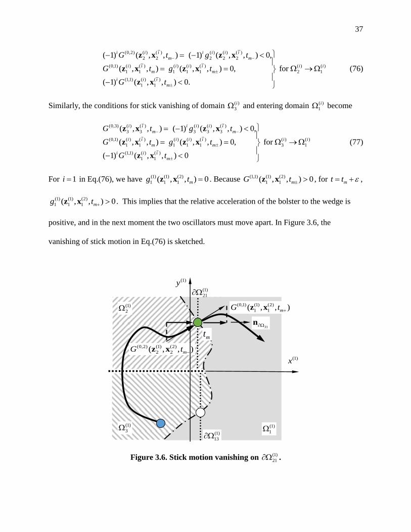
(0,2) ( ) ( ) ( ) ( ) ( )
2 2 2 2 2
(0,1) ( ) ( ) ( ) ( ) ( ) ( ) ( )
1 1 1 1 1 2 1
(1,1) ( ) ( )
1 1
( 1) ( , , ) ( 1) ( , , ) 0,
( , , ) ( , , ) 0, for
( 1) ( , , ) 0.
i i i i i i i
m m
i i i i i i i
m m
i i i
m
G t g t
G t g t
G t
z x z x
z x z x
z x
(76)
Similarly, the conditions for stick vanishing of domain ( )
3
i and entering domain ( )
1
i become
(0,3) ( ) ( ) ( ) ( ) ( )
3 3 3 3 3
(0,1) ( ) ( ) ( ) ( ) ( ) ( ) ( )
1 1 1 1 1 3 1
(1,1) ( ) ( )
1 1
( , , ) ( 1) ( , , ) 0,
( , , ) ( , , ) 0, for
( 1) ( , , ) 0
i i i i i i
m m
i i i i i i i
m m
i i i
m
G t g t
G t g t
G t
z x z x
z x z x
z x
(77)
For 1i in Eq.(76), we have (1) (1) (2)
1 1 1( , , ) 0mg t z x . Because (1,1) (1) (2)
1 1( , , ) 0mG t z x , for mt t ,
(1) (1) (2)
1 1 1( , , ) 0mg t z x . This implies that the relative acceleration of the bolster to the wedge is
positive, and in the next moment the two oscillators must move apart. In Figure 3.6, the
vanishing of stick motion in Eq.(76) is sketched.
(1)
2
(1)
3
(1)
21
(1)x
(1)
13
(1)
1
mt31n
(0,2) (1) (2)
2 2( , , )mG t z x
(0,1) (1) (2)
1 1( , , )mG t z x
(1)y
Figure 3.6. Stick motion vanishing on (1)
21 .

38
From Eq.(23), ( ) ( ) ( )g ( , , )i i i t z x is equivalent to ( ) ( ) ( )g ( , , )i i i t z x because ( )i
x is a function of
time and the calculation of (1, ) ( ) ( )( , , , )i iG t
z x from Eq.( 75) is given by
(1, ) ( ) ( ) ( ) ( ) ( ) 2 ( ) ( )
( ) ( ) ( ) ( ) 2 ( )
( , , ) 2 ( ) sin
2 ( ) .
i i i i i i i
i i i i i
G t z z Q t
x x x
z x (77)
Therefore, the function (1, ) ( ) ( )( , , )i iG t
z x is a relative jerk in domain ( )i
. From Eqs.(29) and
(31), the relative jerk is given by
( ) ( ) ( ) ( ) 2 ( ) ( )
( ) ( ) ( ) ( ) 2 ( )
( ) 2 ( ) sin
2 ( ) .
i i i i i i
i i i i i
J t z z Q t
x x x
(78)
The function ( ) ( ) ( )g ( , , )i i i t z x is a relative acceleration or a relative force per unit mass. From Luo
(2008) and (2009), the grazing of stick motion requires
( )21
(0,1) ( ) ( ) ( ) ( ) ( )
1 1 1 1 1
(1,1) ( ) ( ) ( ) ( ) ( )
1 1 1 1 1
(0,2) ( ) ( ) ( ) ( ) ( )
2 2 2 2 2
(1,2) ( ) ( )
2 2
( , , ) ( , , ) 0
( , , ) ( 1) ( , , ) 0for
( , , ) ( , , ) 0
( 1) ( , , ) 0
i
i i i i i
m m
i i i i i i
m m
i i i i i
m m
i i i
m
G t g t
G t Dg t
G t g t
G t
z x z x
z x z xn
z x z x
z x
( )
1 ,i (79)
(31
(0,1) ( ) ( ) ( ) ( ) ( )
1 1 1 1 1
(1,1) ( ) ( ) ( ) ( ) ( )
1 3 1 1 3
(0,3) ( ) ( ) ( ) ( ) ( )
3 3 3 3 3
(1,3) ( ) ( )
3 1
( , , ) ( , , ) 0
( , , ) ( 1) ( , , ) 0for
( , , ) ( , , ) 0
( 1) ( , , ) 0
i
i i i i i
m m
i i i i i i
m m
i i i i i
m m
i i i
m
G t g t
G t Dg t
G t g t
G t
z x z x
z x z xn
z x z x
z x
)
( )
1 .i (80)
In Figure 3.7, an illustration of grazing motion is presented to help understand the analytical
grazing conditions in Eq.(80). The blue circle designates the starting point within the stick
domain (1)
2 . With (0,2) (1) (2)
2 2( , , ) 0G t z x , the solid black curve approaches the boundary (1)
21 .
Upon reaching the boundary at time mt , (0,2) (1) (2)
2 2( , , ) 0mG t z x . However (1,2) (1) (2)
2 2( , , ) 0mG t z x
so for mt t , (0,2) (1) (2)
2 2( , , ) 0mG t z x will be true. With the stick motion conditions of

39
Eq.(73), the wedge and bolster will remain in 2 . Furthermore, with (0,2) ( )( , ) 0i
m mG t z the
solid black curve in Figure 3.7 will move to back to domain 2 to keep contact without
interaction to the boundary 21 .
( )
2
i
( )
3
i
(1)
21
(1)
13(1)
1
31n mt
(0,2) (1) (1)
2 2( , , )mG t z x
(0,2) (1) (1)
2 2( , , )mG t z x (1)x
(1)y
Figure 3.7: Grazing of stick motion at ( )
21
i .

40
CHAPTER IV
MOTION DESCRIPTION
To discuss periodic impacting chatter with and without stick in the freight train
suspension system, the mapping structure will be introduced through the boundaries. Before the
mapping structure for a prescribed impacting chatter motion is developed, the switching planes
will be defined first, and from the switching planes, the basic mappings will be developed for the
mechanical model. Basic mappings will also be defined in the relative frame. A bifurcation
scenario will be presented to illustrate complicated motions of the freight train suspension
system.
4.1 Switching Sets and Basic Mappings
For a periodic motion with stick motion in the train suspension system, consider the case
when the bolster and wedges are sticking together always. Since the discontinuity results from
the friction force sign change, the switching planes for stick are defined at zero velocity.
However, from Luo & Gegg (2005) and Luo (2009) and (2012), the oscillators may stick to the
velocity boundary. From Eq. (19), the corresponding switching planes are defined as
( ) ( ) ( ) ( ) ( ) ( ) ( )
23
( ) ( ) ( ) ( ) ( ) ( ) ( )
32
( ) ( ) ( ) ( ) ( ) ( ) ( )
0
( , , , ) 0, 0 ,
( , , , ) 0, 0 ,
( , , , ) , 0 .
i i i i i i i
k k k k k k k
i i i i i i i
k k k k k k k
i i i i i i i
k k k k k k k
t x x x x x x
t x x x x x x
t x x x x x x
(81)
The switching planes ( )
23
i and ( )
32
i define the switching sets for the zero velocity boundary
having a positive or negative displacement, respectively. The switching plane ( )
0
i defines the
switching set for the zero velocity boundary to stuck with two side walls.
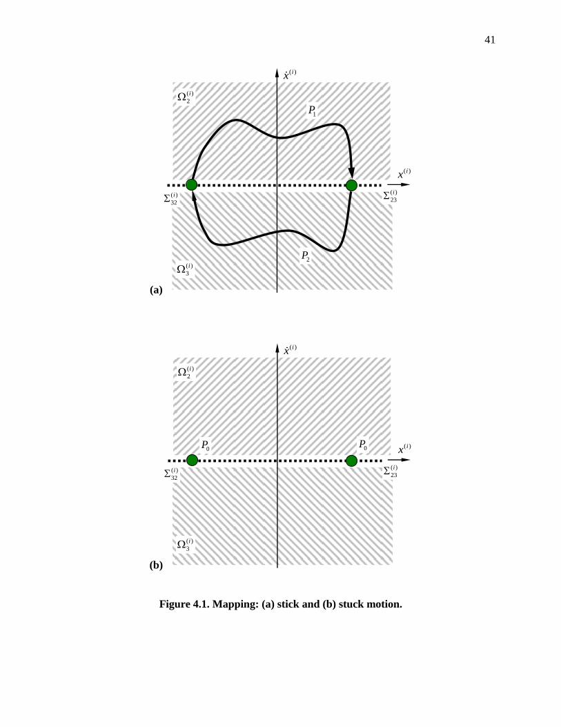
41
(a)
( )ix
1P
2P
( )ix
( )
2
i
( )
3
i
( )
32
i( )
23
i
(b)
( )ix
0P0P ( )ix
( )
2
i
( )
3
i
( )
32
i( )
23
i
Figure 4.1. Mapping: (a) stick and (b) stuck motion.

42
From the above switching planes, the mappings are defined as
( ) ( ) ( ) ( ) ( ) ( )
0 0 0 1 32 23 2 23 32: , : , : .i i i i i iP P P (82)
The 0P mapping is where the bolster and two wedges are stuck together, but the combined
system is also stuck to the wall (i.e., the bolster does not move). The other two mappings ( 1P and
2P ) are stick motions with positive and negative velocities, respectively. The switching phase is
defined by mod( ,2 )k kt . To illustrate the stick mappings, 1P and
2P are illustrated in
Figure 4.1 by the curves with positive and negative velocity, respectively. Since velocity is zero
for the stuck mapping 0P , the entire mapping exists as a single point on the phase plane. But,
with varying time, the force will be changed, and the stuck motion will start once the force
condition is satisfied.
From the discontinuous boundaries, the switching plane based on the impacting chatter
boundary is defined as
( ) ( ) ( ) ( ) ( ) ( ) ( ) ( )
1 ( , , , ) ,i i i i i i i i
k k k k k k k kt x x x x x x x (83)
for ( {1,2}i,i and i i ). From now on, ( ) ( ) ( )i i
k kx x t and ( ) ( ) ( )i i
k kx x t are switching
displacement and velocity on the separation boundary at time kt .
Based on the above definition of switching plane, a single mapping for impacting chatter is
defined in the absolute frame as
( ) ( )
5 1 1: .i iP (84)
In Figure 4.2, the 5P map is illustrated through the curves that connect the switching planes ( )
1
i
.
The bolster and two wedges come into contact with repeated impacts but do not stick together
(i.e., always free-flight).

43
(1)y
(1)x
(1)
1(1)
1
(1)
1(1)
1
5P
5P
5P
Figure 4.2. The free flight to impacting chatter map 5P .
For the passable stick boundaries ( )
21
i and ( )
13
i , the corresponding switching sets are
defined as
( ) ( ) ( ) ( ) ( ) ( ) ( ) ( )
21
( ) ( ) ( ) ( ) ( ) ( ) ( ) ( )
13 1
( , , , ) , 0 ,
( , , , ) , 0 .
i i i i i i i i
k k k k k k k k
i i i i i i i i
k k k k k k k
t x x x x x x x
t x x x x x x x
(85)
Since the stick boundaries separate the free-flight and stick domains, the mappings for other
motions in the mixed domains are defined as
( ) ( ) ( ) ( )
3 32 21 4 21 1
( ) ( ) ( ) ( )
5 1 1 6 13 32
: , : ,
: , : .
i i i i
i i i i
P P
P P
(86)
Upon stick motion separation the motion is described by 3P , and for repeated impacts the motion
is described by 4P . The mappings based on the sticking and impacting switching planes are
presented in Figure 4.3.
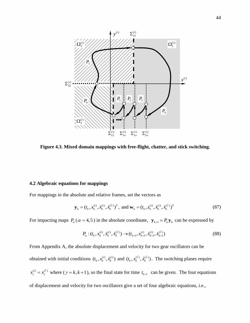
44
( )
2
i
( )
3
i
( )
23
i( )ix
( )
1
i
( )
1
i
( )
1
i
( )
21
i
( )
13
i
( )
32
i
5P5P5P6P
4P
3P
( )
1
i
( )iy
Figure 4.3. Mixed domain mappings with free-flight, chatter, and stick switching.
4.2 Algebraic equations for mappings
For mappings in the absolute and relative frames, set the vectors as
( ) ( ) ( ) T ( ) ( ) ( ) T( , , , ) , and ( , , , )i i i i i i
k k k k k k k k k kt x x x t z x x y w (87)
For impacting maps P ( 4,5 ) in the absolute coordinate, 1k kP y y can be expressed by
( ) ( ) ( ) ( ) ( ) ( )
1 1 1 1: ( , , , ) ( , , , )i i i i i i
k k k k k k k kP t x x x t x x x (88)
From Appendix A, the absolute displacement and velocity for two gear oscillators can be
obtained with initial conditions ( ) ( )( , , )i i
k k kt x x and ( ) ( )( , , )i i
k k kt x x . The switching planes require
( ) ( )i ix x where ( , 1k k ), so the final state for time 1kt can be given. The four equations
of displacement and velocity for two oscillators give a set of four algebraic equations, i.e.,

45
( )
1( , ) 0k k
f y y , (89)
where
( ) ( ) ( ) ( ) ( ) T
1 2 3 4( , , , )f f f f f . (90)
For the impact mapping itself, Eq.(86) can be determined from the impact relationships as
( )
1 1
( ) ( ) ( )
2 1
( ) ( ) ( ) ( ) ( ) ( )
3 1 1 2
( ) ( ) ( ) ( ) ( ) ( )
4 1 1 2
,
,
k k
i i
k k
i i i i i
k k k
i i i i i
k k k
f t t
f x x
f x I x I x
f x I x I x
(91)
For the stick motion, the displacement and velocity of the ith oscillator will be adopted. In
addition, the stick vanishing conditions in Eqs.(75) and (77) will be used.
( ) ( )
1 1
( ) ( ) ( ) ( )
1 1 1 1
,
( , , , ) 0.
i i
k k
i i i i
k k k k
x x
g t x x x
(92)
With the condition ( ) ( )i ix x for ( , 1k k ), the algebraic equations in Eq.(90) can be
obtained. If a mapping starts or ends at the stick boundary, the corresponding displacement plus
the following equation can be employed to obtain Eq.(92).
( ) ( ) for { , 1}i ix x k k (93)
Based on the relative coordinate ( ) ( )( , )i iz z , the relative displacement and velocity can be used
with the initial condition ( ) ( )(t , , )i i
k k kz z on the switching boundary. The displacement and velocity
with an initial condition ( ) ( )(t , , )i i
k k kx x can be given. With conditions ( ) 0iz for ( , 1k k ),
the relative and absolute displacements and velocities generate a set of four algebraic equations
as
( )
1( , ) 0k k
h w w (94)
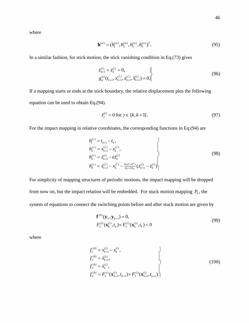
46
where
( ) ( ) ( ) ( ) ( ) T
1 2 3 4( , , , ) .h h h h h (95)
In a similar fashion, for stick motion, the stick vanishing condition in Eq.(73) gives
( ) ( )
1
( ) ( ) ( ) ( )
1 1 1 1
0,
( , , , ) 0.
i i
k k
i i i i
k k k k
z z
g t x x x
(96)
If a mapping starts or ends at the stick boundary, the relative displacement plus the following
equation can be used to obtain Eq.(94).
( ) 0 for { , 1}.iz k k (97)
For the impact mapping in relative coordinates, the corresponding functions in Eq.(94) are
2
1 2
( )
1 1
( ) ( ) ( )
2 1
( ) ( ) ( )
3 1
(1 )( ) ( ) ( ) ( ) ( )
4 1 12
,
,
( )i i
k k
i i
k k
i i
k k
mi i i i
k k k km m
h t t
h x x
h z ez
h x x z z
(98)
For simplicity of mapping structures of periodic motions, the impact mapping will be dropped
from now on, but the impact relation will be embedded. For stuck motion mapping 0P , the
system of equations to connect the switching points before and after stuck motion are given by
(0)
1
( ) ( ) ( ) ( )
2 3
( , ) 0,
( , ) ( , ) 0
k k
i i i i
k k k kF t F t
f y y
x x (99)
where
(0) ( ) ( )
1 1
(0) ( )
2 1
(0) ( )
3
(0) ( ) ( ) ( ) ( )
4 2 1 1 3 1 1
,
,
,
( , ) ( , ).
i i
k k
i
k
i
k
i i i i
k k k k
f x x
f x
f x
f F t F t
x x
(100)

47
4.3 Mapping structures
To investigate periodic motions in such a freight train suspension system, the notation for
mapping actions of basic mappings is introduced as in Luo (2009) and (2012)
1 0 1 0k kn n n n n nP P P P (101)
where the mapping jnP ( 0,1, ,6jn , 1,2, ,j k ) is defined in the previous section.
Consider a generalized mapping structure as
4 3 2 1 31 4 3 2 1 3141 21 11 41 21 11(65 432 1 0 ) (65 432 1 0 ) (65 432 1 0 ) (65 432 1 0 )k k k k k k k k k kk k k k k ks s s s s s s s
s terms
P P P
(102)
where ( {0, },k 1,2, , s , 1,2,3,4 ). From the generalized mapping structure,
consider a simple mapping structure of periodic motions for impacting chatter with stick and
stuck motion. For instance, the mapping structure is
6 4 3 065 430 5m mP P P P P P (103)
where 0,m . Such a mapping structure gives ( 1)m impacts on the boundary 1
which are described by mappings. Consider a periodic motion of 65 430mP with period 1 1T k T
( 1k ). If the mapping structure copies itself, the new mapping structure is:
2(65 430) 65 430 65 430m m mP P P (104)
The periodic motion of 2(65 430)mP is obtained during a period of 12T . In a similar fashion, such an
action of mapping structure continues to copy itself with period- 12l T .
1 12 2 2(65 430) (65 430) (65 430)l l lm m m
P P P (105)
As l , a chaotic motion relative to mapping structure 65 430mP is formed. The prescribed chaos
is generated by period-doubling. However, if grazing bifurcation occurs, such a mapping

48
structure may not be copied by itself. The new mapping structures are combined by the two
different mapping structures. For instance,
2 1 2 1
1 1
(65 430)(65 430) 65 430 65 430
(65 430) (65 430) 65 43065 430
,
.
m m m m
ml m m ml
l terms
P P P
P P P
(106)
Such a grazing bifurcation will cause the discontinuity of periodic motions, and chaotic motions
may exist between periodic motions 1(65 430) (65 430)ml mP and 1 1(65 430) (65 430)ml mP . If the wedge and
bolster do not have free-flight motion or remain in stick motion always, the mapping structure
may take the general form
3 3 312 1 2 1 21 112 1 0 2 1 0 2 1 0
k k kk k ks ks k ks
s terms
P P P
(107)
In a similar manner above, the period doubling and grazing bifurcation for stick can be discussed.
4.4 Bifurcation scenario
From the motion mappings, a bifurcation scenario can be presented through the switching
displacements, velocities, and phases of the wedge and bolster. All the numerical computations
are completed from the closed-form solutions in Appendix A. Herein, a set of system parameters
( 1 3,m 2 1,m 1 2 0.1,r r 1 2 20,k k 0 20,A 0.4k 37.5 , and 0.6e ) are
considered to investigate the mechanical model. The impacting chatter with and without stick
varying with excitation frequency are presented in the following figures. The switching phase
k kt , displacement (1)
kx are shown Figure 4.4 while the two switching velocities (1)
ky and
(2)
ky of the bolster and wedges are shown in Figure 4.5. For the range of frequencies labeled
“Chatter w/stick”, (0.001,1.662) , the motion consists of multiple chatter impacts which

49
(a)
(b)
Figure 4.4. Bifurcation scenario for switching: (a) phase and (b) displacement,
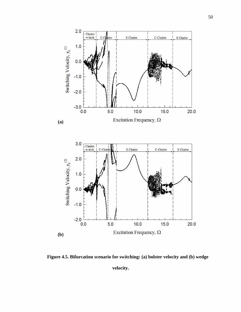
50
(a)
(b)
Figure 4.5. Bifurcation scenario for switching: (a) bolster velocity and (b) wedge
velocity.
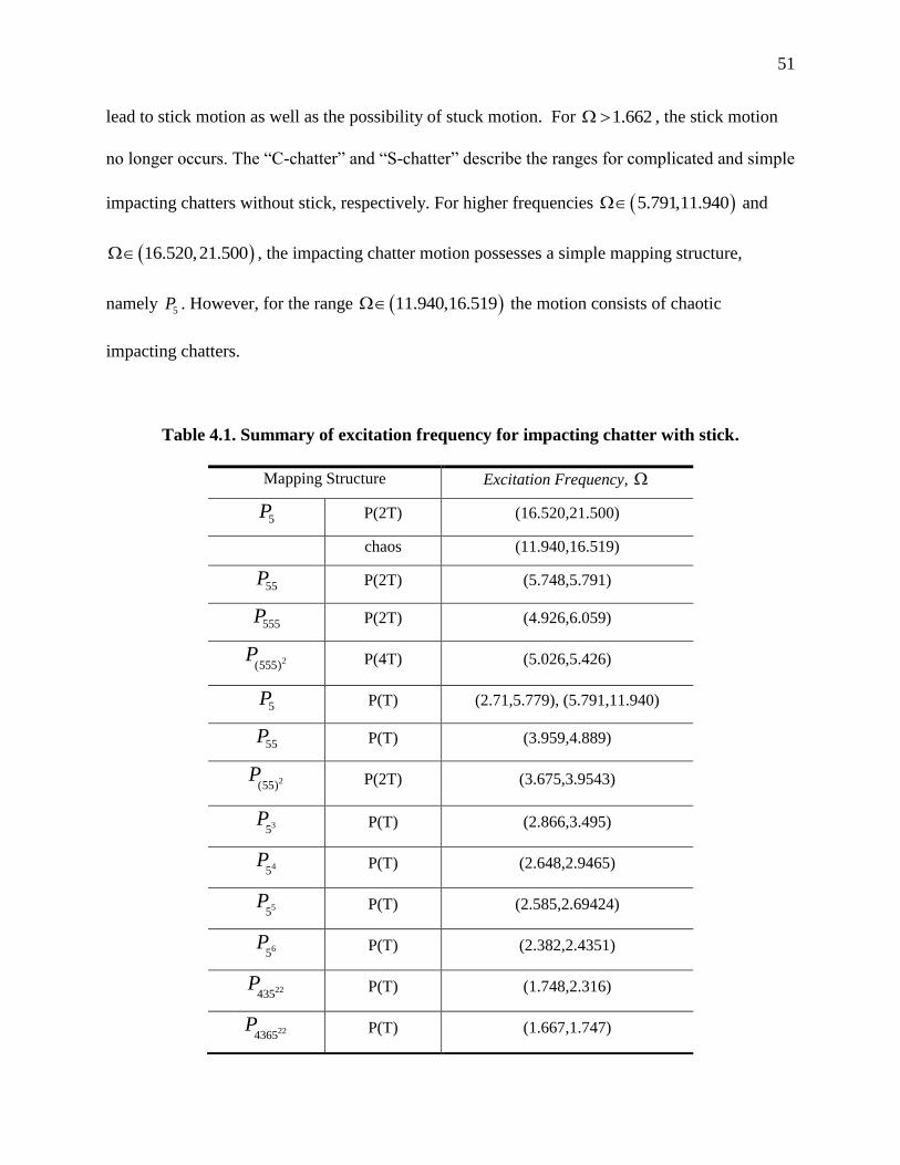
51
lead to stick motion as well as the possibility of stuck motion. For 1.662 , the stick motion
no longer occurs. The “C-chatter” and “S-chatter” describe the ranges for complicated and simple
impacting chatters without stick, respectively. For higher frequencies 5.791,11.940 and
16.520,21.500 , the impacting chatter motion possesses a simple mapping structure,
namely 5P . However, for the range 11.940,16.519 the motion consists of chaotic
impacting chatters.
Table 4.1. Summary of excitation frequency for impacting chatter with stick.
Mapping Structure Excitation Frequency,
5P P(2T) (16.520,21.500)
chaos (11.940,16.519)
55P P(2T) (5.748,5.791)
555P P(2T) (4.926,6.059)
2(555)P P(4T) (5.026,5.426)
5P P(T) (2.71,5.779), (5.791,11.940)
55P P(T) (3.959,4.889)
2(55)P P(2T) (3.675,3.9543)
35P P(T) (2.866,3.495)
45P P(T) (2.648,2.9465)
55P P(T) (2.585,2.69424)
65P P(T) (2.382,2.4351)
22435P P(T) (1.748,2.316)
224365P P(T) (1.667,1.747)
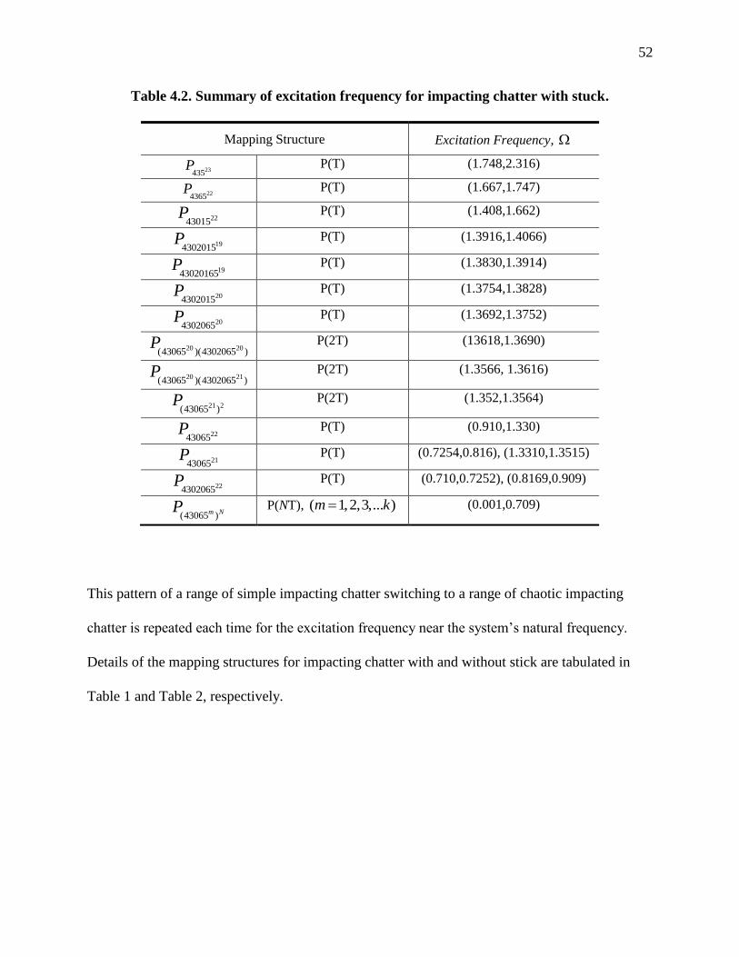
52
Table 4.2. Summary of excitation frequency for impacting chatter with stuck.
Mapping Structure Excitation Frequency,
23435P P(T) (1.748,2.316)
224365P P(T) (1.667,1.747)
2243015P P(T) (1.408,1.662)
194302015P P(T) (1.3916,1.4066)
1943020165P P(T) (1.3830,1.3914)
204302015P P(T) (1.3754,1.3828)
204302065P P(T) (1.3692,1.3752)
20 20(43065 )(4302065 )P P(2T) (13618,1.3690)
20 21(43065 )(4302065 )P P(2T) (1.3566, 1.3616)
21 2(43065 )P P(2T) (1.352,1.3564)
2243065P P(T) (0.910,1.330)
2143065P P(T) (0.7254,0.816), (1.3310,1.3515)
224302065P P(T) (0.710,0.7252), (0.8169,0.909)
(43065 )m NP P(NT), ( 1,2,3,... )m k (0.001,0.709)
This pattern of a range of simple impacting chatter switching to a range of chaotic impacting
chatter is repeated each time for the excitation frequency near the system’s natural frequency.
Details of the mapping structures for impacting chatter with and without stick are tabulated in
Table 1 and Table 2, respectively.

53
CHAPTER V
GENERAL PREDICTION RESULTS
In this Chapter, the analytical prediction of periodic motion will be completed through the
mapping structure, and the corresponding local stability and bifurcation analysis will be carried
out through the eigenvalue analysis. The generalized methodology for analytical prediction and
stability analysis of periodic motions will be presented first. The two periodic motions with and
without stick will be discussed. The switching displacement, velocity, and phase varying with
excitation frequency will be given. Finally, the stability and bifurcation analysis will be
presented through the eigenvalues of the prescribed periodic motions.
5.1 Periodic Motions
From mapping structures of periodic motions, the switching sets for any specific periodic
motion can be determined through solving a set of nonlinear algebraic equations. Consider a
periodic motion of mapping structure4 3 2 1 3141 21 11(65 432 1 0 ) (65 432 1 0 )
k k k k kk k ks s s sP and the following relation
holds.
44 3 2 1 3141 21 11
1 1
(65 432 1 0 ) (65 432 1 0 )2
k k k k k sk k ks s s s
mj
m j
kk s k
P
y y (108)
where ( ) ( ) ( ) T( , , , )yi i i
k k k k kt x x x . A set of vector equations is as

54
4 4
1 1 1 1
2
1
2
2 1
6
2 2 1
, 0,
, 0,
, 0;s s
mj mj
m j m j
k k
k k
k s k k s k
f y y
f y y
f y y
(109)
where ( ) ( ) ( ) ( ) ( ) T
1 2 3 4( , , , )f f f f f is relative to governing equations of mapping P
( 1,2, ,6 ). The periodicity of the period-1 motion per N-periods requires
4
1 1
2
s
mj
m j
kk s k
y y (110)
or
4 4 4
1 1 1 1 1 1
4
1 1
( ) ( ) ( ) ( ) ( ) ( )
2 2 2
2
, , ,
2 .
s s s
mj mj mj
m j m j m j
s
mj
m j
i i i i i i
k k kk s k k s k k s k
kk s k
x x x x x x
t t N
(111)
Solving Eqs.(109) and (110) generates the switching sets for periodic motions. Once the
analytical prediction of any periodic motion is obtained, the corresponding stability and
bifurcation analysis can be completed.
5.2 Stability
The local stability and bifurcation for such a period-1 motion is determined through the
corresponding Jacobian matrix of the Poincaré mapping. From Eq.(109), the Jacobian matrix is
computed by the chain rule,

55
4 3 2 1 3141 21 11
4 3 2 1
(65 432 1 0 ) (65 432 1 0 )
6 5 4 3 2 1 0
1
k k k k kk k ks s s s
m m m m
nk k k k
m
DP DP
DP DP DP DP DP DP DP
(112)
where
( ) ( ) ( )
1 1 1 1
( ) ( ) ( )
( , , , )
( , , , )
i i i
i i i
t x y yDP
t x y y
(113)
for 4
1 1, 1, , 2 1
s
mjm jk k k s k
, and all the Jacobian matrix components can be
computed through Eq.(96). The variational equation for a set of switching points
4
1 1
* *
2 1
{ , , }s
mj
m j
kk s k
y y is
4
1 1
*
2
( ) .s
mj
m j
k kk s k
DP
y y y (114)
A derivation of Eq.(109) is shown in Appendix C. The eigenvalues are computed by
| I | 0.DP (115)
The Jacobian matrix DP is 4x4, and the eigenvalues can be determined by the QR factorization.
A C++ version of the QR factorization is shown in Appendix D. Because DP is a 4x4 matrix,
there are four eigenvalues. If the four eigenvalues lie inside the unit circle, then the period-1
motion is stable. If one of them lies outside the unit circle, the periodic motion is unstable.
i. If the eigenvalues to be
1, 1,2,3,4 .j j (116)
the periodic motion is table.
ii. If the magnitude of any eigenvalue is greater than one,
| | 1, {1,2,3,4}j j (117)

56
the periodic motion is unstable. The corresponding bifurcation conditions are summarized as
follows.
i. For | | 1 3,4j j and real 1,2j j , if
max{ , 1,2} 1, min{ , 1,2} 1,1j jj j , (118)
then the saddle-node (SN) bifurcation occurs; if
min{ , 1,2} 1, max{ , 1,2} 1,1j jj j , (119)
then the period-doubling bifurcation occurs.
ii. For | | 1 3,4j j and complex 1,2j j , if
| | 1 1,2 ,j j (120)
then the Neimark bifurcation occurs.
5.3 Impacting Chatter Prediction
Using the mapping structure in Eq.(102), all the periodic motions for the entire range of
excitation frequency can be determined analytically. The mapping structure gives the nonlinear
algebraic equations similar to Eqs.(99) and (100), which can be solved by the Newton-Raphson
method. Once the first solution is obtained, the rest of the solutions with varying parameters can
be determined through the corresponding mapping structure. The generic parameters ( 1 3,m
2 1,m 1 2 0.1,r r 1 2 20,k k 0 20,A 0.4k 37.5 , and 0.6e ) are also used for
the analytical prediction of periodic motions. Firstly, the analytical prediction of the simplest
periodic motion 5P is shown in Figures 5.1 and 5.2. The switching phase and displacement of
57
the bolster (i.e., (1)
ky ) is plotted in Figure 5.1(a) and (b), respectively. The solid black curve
represents the stable periodic switching phase and displacement while the red dashed curve
represents the unstable periodic switching solutions. Also, the solid blue curve describes the
switching sets for 55P after period doubling motion occurs at 5.80 . Note, at switching
points, the switching phase and displacement of the bolster and wedge are identical since they
make contact at (1) (2)
k kx x and the wedges have no forcing function. The switching velocities for
each oscillator is presented in Figure 5.2. Due to the impact relationships defined in Chapter 1,
the switching velocity sets are only recorded just before impact.
The corresponding eigenvalues to the analytical prediction of 5P periodic motion are
presented in Figure 5.3. From local stability analysis gives the excitation frequency range for
stable and unstable periodic motion. The stable range for periodic motion 5P is found for the
three sets 16.520,21 0( ).50 , 2.71,5. 9( )77 , and 5.791,11. 0( )94 . Again, the solid
black curves and dashed red curves correspond to stable and unstable switching sets,
respectively. Note, the vertical dashed lines show the bifurcation points. Also, “GB” stands for
grazing bifurcation, “NB” stands for Neimark bifurcation, and “PD” stands for period doubling.
From Figure 5.3(a), period doubling occurs when the real part of one eigenvalue equals -1.0 at
5.791 . The range for stable 55P is 5.748,5. 1( )79 with the motion disappearing from a
grazing bifurcation at 5.748 . In Figure 5.4, the eigenvalue magnitudes are plotted to help
show the Neimark bifurcation points. To verify the stability of the period doubling solution 55P ,
the corresponding eigenvalues are plotted in Figure 5.4(b).

58
(a) Excitation Frequency,
0.0 6.0 12.0 18.0 24.0
Sw
itch
ing
Ph
ase,
mo
d(
t k, 2
)
0.0
2.0
4.0
6.0 GB NB NBNBNBPD
5.72 5.76 5.803.0
3.2
3.4 PDGB
(b) Excitation Frequency,
0.0 6.0 12.0 18.0 24.0
Sw
itch
ing
Dis
pla
cem
ent
x k(1)
-2.0
2.0
6.0
10.0GB NBNB NBNBPD
5.72 5.76 5.800.36
0.40
0.44
PDGB
Figure 5.1. Analytical prediction of (a) switching phase and (b) displacement for 5P .

59
(a) Excitation Frequency,
0.0 6.0 12.0 18.0 24.0
Sw
itch
ing
Vel
oci
ty, y k(1
)
-18.0
-13.0
-8.0
-3.0
2.0GB NB NBNBNBPD
5.72 5.76 5.80-2.8
-2.0
-1.2 PDGB
(b) Excitation Frequency,
0.0 6.0 12.0 18.0 24.0
Sw
itch
ing
Vel
oci
ty,
y k(2)
-4.0
0.0
4.0
8.0GB NB NBNBNBPD
PDGB
5.72 5.76 5.800.8
1.4
2.0
Figure 5.2. Analytical prediction of switching velocities for 5P .
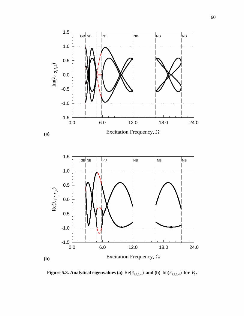
60
(a) Excitation Frequency,
0.0 6.0 12.0 18.0 24.0
Im(
-1.5
-1.0
-0.5
0.0
0.5
1.0
1.5GB NBNB NBPD NB
(b) Excitation Frequency,
0.0 6.0 12.0 18.0 24.0
Re(
-1.5
-1.0
-0.5
0.0
0.5
1.0
1.5GB NBNB NBNB PD
Figure 5.3. Analytical eigenvalues (a) 1,2,3,4Re( ) and (b) 1,2,3,4Im( ) for 5P .

61
(a) Excitation Frequency,
0.0 6.0 12.0 18.0 24.0
Mag
nit
ud
e o
f E
igen
val
ues
,
0.2
0.4
0.6
0.8
1.0
1.2
1.4GB NBNB NBPD NB
(b) Excitation Frequency,
5.74 5.76 5.78 5.80
Mag
nit
ud
e o
f E
igen
val
ues
,
0.0
0.2
0.4
0.6
0.8
1.0
1.2GB SN
Figure 5.4. Magnitude of eigenvalues for (a) 5P and (b) 55P .

62
5.4 Impacting Chatter with Stick and Stuck Prediction
The analytical prediction of periodic motions with stick and stuck motion is also given
herein. Using the generic parameters ( 1 3,m 2 1,m 1 2 0.1,r r 1 2 20,k k
0 20,A
0.4k 37.5 , and 0.6e ), the corresponding switching sets varying with excitation
frequency are presented in Figures 5.5 through 5.9. Because the computational time is very
consuming, the impacting chatters with stick and stuck are predicted only in the range of
excitation frequency (0.710,2.316) . In Figure 5.5(a), the switching phase is plotted for the
complete set of impacting chatter with stick and stuck. For the range, (1.667,2.316) there is
impacting chatter and stick motion. On the other hand, for the range (0.710,1.662) there is
both impacting chatter with stick as well as stuck motion. Recall, stuck motion is defined by the
0P map. Due to the complicated motion switching, Figure 5.5(b) describes in more detail the
switching phase solutions and mapping structures for the excitation frequency (1.35,1.40) .
The eigenvalues of impacting chatter with stick and stuck motion are presented in Figure
5.9. Note that eigenvalues 3,4 are necessarily zero for the entire range of stick motion.
Moreover, for stuck motion, the eigenvalues 2,3,4 are necessarily zero. In Figure 5.9(a), the
vertical dashed lines labeled “SB” represents the stick bifurcations. On the far right, the
impacting chatter with stick disappears after 2.316 . Consider the range (1.408,1.662)
with mapping structure 2243015P , the end of stuck motion occurs with a saddle node bifurcation at
1.662 . Finally, in impacting chatter to stick motion computation, the computational criterion
(1) (2) 6| | 10k kx x was embedded as a tolerance to minimize the number of impacts before
considering the stick conditions.
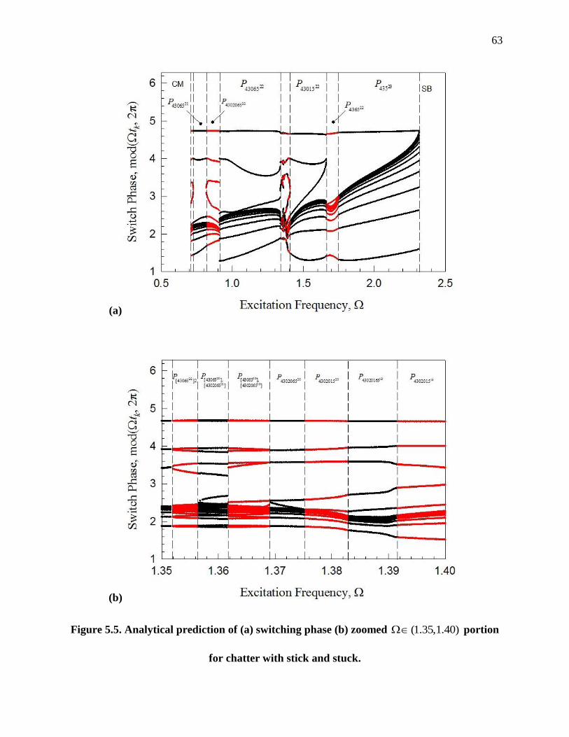
63
(a)
(b)
Figure 5.5. Analytical prediction of (a) switching phase (b) zoomed (1.35,1.40) portion
for chatter with stick and stuck.

64
(a)
(b)
Figure 5.6. Analytical prediction of (a) switching displacement and (b) zoomed
(1.35,1.40) portion for chatter with stick and stuck.

65
(a)
(b)
Figure 5.7. Analytical prediction of (a) switching velocity (1)y and (b) zoomed
(1.35,1.40) portion for chatter with stick and stuck.

66
(a)
(b)
Figure 5.8. Analytical prediction of (a) switching velocity (2)y and (b) zoomed
(1.35,1.40) portion for chatter with stick and stuck.

67
(a) Excitation Frequency,
0.5 1.0 1.5 2.0 2.5
Mag
of
eig
env
alu
es,|
0.0
0.2
0.4
0.6
0.8
1.0
1.2
SBSBSNSBSBSB SBSB
(b) Excitation Frequency,
1.35 1.36 1.37 1.38 1.39 1.40
Mag
of
eig
env
alu
es,|
0.0
0.2
0.4
0.6
0.8
1.0
1.2
22[43065 ]2P 20
21[43065 ],
[4302065 ]
P204302065
P 204302015P 1943020165
P20
20[43065 ],
[4302065 ]
P194302015
P
SBSBSBSNSBSBSN
Figure 5.9. Magnitude of eigenvalues for chatter with stick and stuck.

68
5.5 Numerical Simulation of Periodic Chatter
Numerical illustrations of periodic motions will help one better understand the motion
mechanisms of such a mechanical model for a train suspension system. From the analytical
prediction of simple impact chatter, the periodic motions will be plotted to illustrate the basic
impact phenomena. In addition, the analytical condition for stick motion will be shown to not be
satisfied during simple impacting chatter. For the parameters ( 1 3,m 2 1,m 1 2 0.1,r r
1 2 20,k k 0 20,A 0.4k 37.5 , and 0.6e ), consider the excitation frequency
6.0 . The analytical prediction gives the initial condition (i.e., 0 =0.54879846t
(1)
0 0.3097066x , (2)
0 0.3097066x , (1)
0 0.26900707y , (2)
0 -1.51636088y ) for the stable
simple periodic impact 5P .
With displacement and velocity time-histories, trajectories of the wedge and bolster are
presented in Figures 5.10 and 5.11. All the responses of the bolster and wedge are represented by
the thick and thin curves, respectively. The switching points before and after impacts are
represented by the small circles. The large circle designates the initial condition for starting
simulation while the vertical dashed line describes one period. From Figure 5.10(a), the bolster
and wedge impact when their displacements are equal causing a velocity jump as seen in Figure
5.10(b). To verify the periodicity of this simple impact chatter, Figure 5.11 shows the bolster and
wedge phase plane trajectories for 5P . The single loop and velocity jump is observed for both the
wedge and bolster. In Figure 5.12, the relative force and jerk are plotted to show why the wedge
and bolster do not stick together. After impact, (1) 0g and (2) 0g . This means that the
acceleration of the bolster is greater than that of the wedge indicating that the bolster will tend to
move apart from the wedge (i.e., (1) (2)x x which yields a positive relative velocity).

69
(a) Time, s
0.0 1.0 2.0 3.0
Dis
pla
cem
ent,
x(i
)
-0.6
-0.3
0.0
0.3
0.6
x(1)
x(2)
1T
(b) Time, s
0.0 1.0 2.0 3.0
Vel
oci
ty, y(i
)
-3.0
-1.5
0.0
1.5
3.0
y(1)
1T
y(2)
Figure 5.10. Displacement and velocity response for simple impacting chatter 5P .
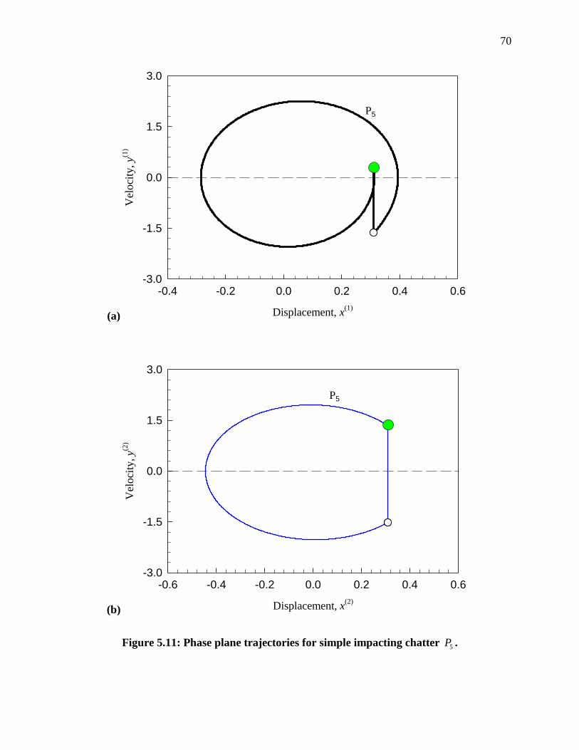
70
(a) Displacement, x(1)
-0.4 -0.2 0.0 0.2 0.4 0.6
Vel
oci
ty,
y(1)
-3.0
-1.5
0.0
1.5
3.0
P5
(b) Displacement, x(2)
-0.6 -0.4 -0.2 0.0 0.2 0.4 0.6
Vel
oci
ty, y(2
)
-3.0
-1.5
0.0
1.5
3.0
P5
Figure 5.11: Phase plane trajectories for simple impacting chatter 5P .

71
(a) Time, s
0.0 1.0 2.0 3.0
Rel
ativ
e F
orc
e, g
(i)
-20.0
-10.0
0.0
10.0
20.01T
g(1)
g(2)
(b) Time, s
0.0 1.0 2.0 3.0
Rel
ativ
e Je
rk, j(i
)
-100.0
-50.0
0.0
50.0
100.01T
j(1)
j(2)
Figure 5.12: Relative force and jerk response for simple for simple impacting chatter 5P .

72
5.6 Numerical Simulation of Chatter with Stick and Stuck Motion
The impacting chatter with stick and stuck motion for the train suspension model will be
discussed through the mapping structure of 215 4306P . For 1.35 , the same parameters as before
( 1 3,m 2 1,m 1 2 0.1,r r 1 2 20,k k
0 20,A 0.4k 37.5 , and 0.6e ) will be
adopted for this illustration. From the analytical prediction, the initial condition is selected from
the switching point 0 1.78307254t , (1) (2)
0 0 -0.09712064x x , and (1) (2)
0 0 -0.062413071y y .
From such an initial condition, the bolster and wedge begin with stick motion. During the stick
motion, the two become stuck having zero velocity and acceleration. After a brief moment, they
continue with stick motion until the analytical conditions allow for the wedge and bolster to
separate. After the stick vanishes, the two oscillators endure free-flying motion. Eventually they
make contact with repeated impacts until finally (1) (2)
k ky y and stick motion is observed.
In Figure 5.13 the displacement and velocity trajectories are presented. The shaded area
is used for stick motion, and the letters “SSP” and “SEP” represent the stick motion starting and
ending point, respectively. The vertical dashed lines define the boundaries for stick and stuck
motion. Accordingly, the letters “WS” describe the section of wall stuck motion. In Figure
5.13(a), the displacement responses of the bolster and wedge are presented. After stick motion,
the thick black curve and the thin blue curve describe the separate free-flight motions of the
bolster and wedge, respectively. Before stick motion is observed again, 21 impacts occur. To
further confirm the impacts, velocity responses for each oscillator are presented in Figure
5.13(b). Notice, during the wall stuck motion, the velocity is zero and the displacement remains
constant. Also, as seen in the acceleration time-history, Figure 5.14(a) shows the acceleration to
be zero during wall stuck motion. Near the end of the free-flight motion, the acceleration (1) 0a

73
and (2) 0a is observed. This explains why the bolster and wedge are headed for collision, (i.e.,
the bolster’s velocity is decreasing while the wedge’s velocity is speeding up). After enough
collisions to satisfy the condition (1) (2)y y , Figure 5.14(b) shows the normal Force between the
wedge and bolster. At the onset and during stick motion, the normal force is positive. However,
at stick motion vanishing, the normal force reduces to zero. Finally, the mapping structure can be
realized through the phase plane trajectories of the bolster and wedge as shown in Figure 5.15.
For a further understanding of the motion phenomena associated with the train suspension
model, the analytical conditions introduced in Chapter 3 must be examined. In Figure 5.16(a), the
g-function for wall stuck is plotted within the shaded region of stick motion. Observe that
(1)
2 0F and (1)
3 0F for the duration of wall stuck. For vanishing stuck (1)
2 0F and (1)
3 0F ;
however in Figure 5.16(b), (2,1)
1 0G which means in the next moment (1)
2 0F thus satisfying
the analytical vanishing stuck conditions. Next consider the motion mechanisms of stick motion.
On the switching boundary with (1) (2)
k ky y , the stick motion requires (1) ( ) 0kg t . In Figure
5.17(a), the relative force (1) 0g is satisfied. In other words, the bolster tends to push down
relative to the wedge. With (2) 0g , the wedge is pushing up relative to the bolster. For the
vanishing of stick motion, it can be observed that the relative force (1) 0g at the switching
boundary. In Figure 5.17(b), the corresponding relative jerk (1) 0J which means that for
kt t , (1) 0g . Note, during stick motion, the relative displacement and velocity are zero. At
the next moment with a positive relative force, (1) (1) (2) 0z y y which means
(1) (1) (2) 0z x x , (i.e., (1) (2)x x ). In other words, the bolster and wedge lie in the state of
free-flying motion, and the stick disappears.

74
(a) Time, s
0.0 2.0 4.0 6.0 8.0 10.0
Dis
pla
cem
ent,
x(i
)
-0.2
0.0
0.2
0.4
x(1)
x(2)
1T
SSP SSP
SEP SEP
WS WS
(b) Time, s
0.0 2.0 4.0 6.0 8.0 10.0
Vel
oci
ty, y(i
)
-0.6
-0.3
0.0
0.3
0.6
y(1)
1T
WS WS
SSP SSP
SEP SEP
y(2)
Figure 5.13. Displacement and velocity response for impacting chatter with stick and stuck
motion 215 4306P .

75
(a) Time, s
0.0 2.0 4.0 6.0 8.0 10.0
Acc
eler
atio
n, a
(i)
-3.0
-1.5
0.0
1.5
3.01T
SSP SSP
SEP
WS WS
SEP
a(2)
a(1)
(b) Time, s
0.0 2.0 4.0 6.0 8.0 10.0
No
rmal
Fo
rce,
N
-2.0
2.0
6.0
10.01T
SSP
SEP
SSP
SEP
WS WS
Figure 5.14. Acceleration and Normal Force response for impacting chatter with stick and
stuck motion 215 4306P .

76
(a) Displacement, x(1)
-0.2 -0.1 0.0 0.1 0.2 0.3
Vel
oci
ty,
y(1)
-0.6
-0.3
0.0
0.3
0.6
P521
P3
P0
P4
P6
(b) Displacement, x(2)
-0.2 -0.1 0.0 0.1 0.2
Vel
oci
ty, y(2
)
-0.6
-0.3
0.0
0.3
0.6
P521
P3
P0
P4
P6
Figure 5.15. Phase plane trajectories of bolster and wedge for impacting chatter with stick
and stuck motion 215 4306P .

77
(a) Time, s
0.0 2.0 4.0 6.0 8.0 10.0
Stu
ck F
unct
ion,
F(1
)
-1.50
-0.75
0.00
0.75
1.50
F3
(1)
1T
WSWS
F2
(1)
(b) Time, s
0.0 2.0 4.0 6.0 8.0 10.0
Stu
ck F
unct
ion,
G1
(,1
)
0.0
1.0
2.0
3.0
4.0
5.0
G1
(2,1)
1T
WSWS
G1
(3,1)
Figure 5.16. First and second order stuck condition function for motion 215 4306P .

78
(a) Time, s
0.0 2.0 4.0 6.0 8.0 10.0
Rel
ativ
e F
orc
e, g
(i)
-6.0
-3.0
0.0
3.0
6.01T
g(1)
g(2)
SSP SSP
SEP SEP
WS WS
(b) Time, s
0.0 2.0 4.0 6.0 8.0 10.0
Rel
ativ
e Je
rk,
J(i)
-15.0
-10.0
-5.0
0.0
5.0
10.0
15.01T
J(1)
J(2)
SEPSSP SSPSEP
WS WS
Figure 5.17. Relative force and jerk time-history for 215 4306P .
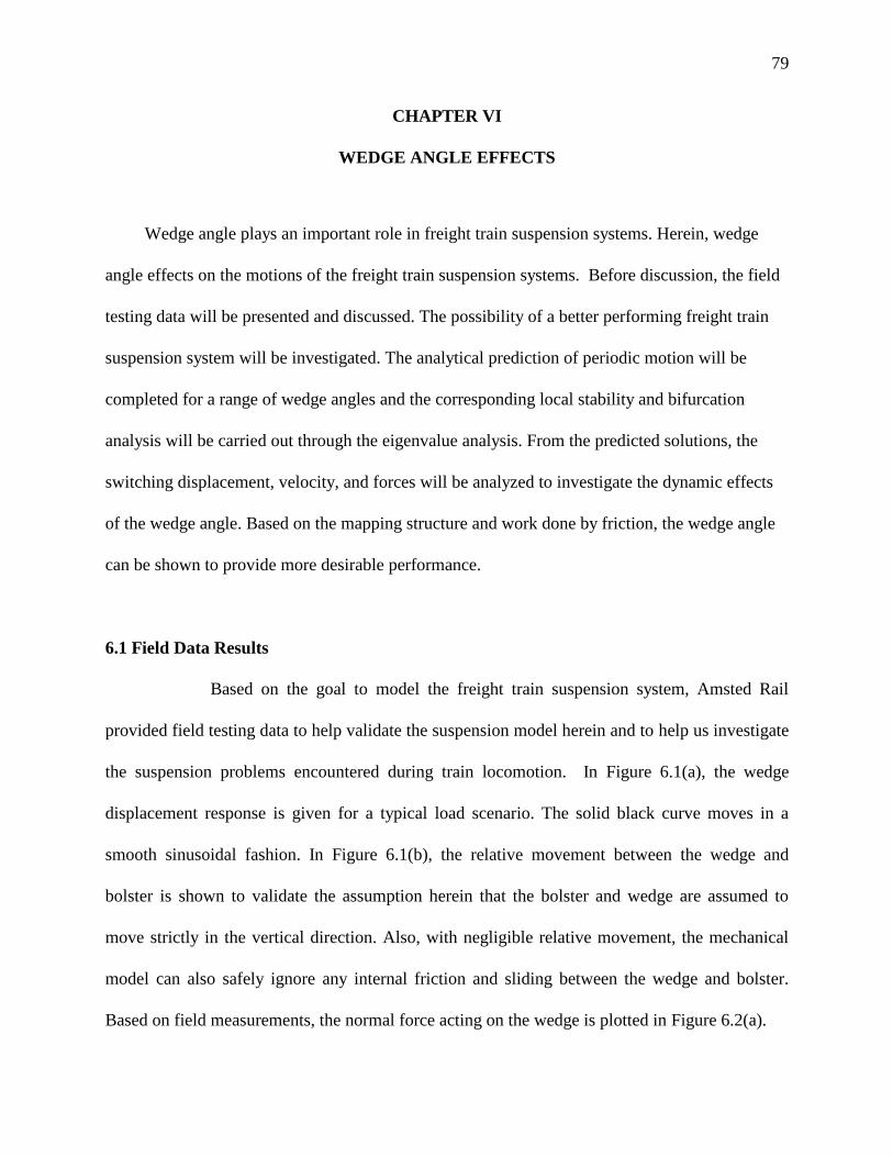
79
CHAPTER VI
WEDGE ANGLE EFFECTS
Wedge angle plays an important role in freight train suspension systems. Herein, wedge
angle effects on the motions of the freight train suspension systems. Before discussion, the field
testing data will be presented and discussed. The possibility of a better performing freight train
suspension system will be investigated. The analytical prediction of periodic motion will be
completed for a range of wedge angles and the corresponding local stability and bifurcation
analysis will be carried out through the eigenvalue analysis. From the predicted solutions, the
switching displacement, velocity, and forces will be analyzed to investigate the dynamic effects
of the wedge angle. Based on the mapping structure and work done by friction, the wedge angle
can be shown to provide more desirable performance.
6.1 Field Data Results
Based on the goal to model the freight train suspension system, Amsted Rail
provided field testing data to help validate the suspension model herein and to help us investigate
the suspension problems encountered during train locomotion. In Figure 6.1(a), the wedge
displacement response is given for a typical load scenario. The solid black curve moves in a
smooth sinusoidal fashion. In Figure 6.1(b), the relative movement between the wedge and
bolster is shown to validate the assumption herein that the bolster and wedge are assumed to
move strictly in the vertical direction. Also, with negligible relative movement, the mechanical
model can also safely ignore any internal friction and sliding between the wedge and bolster.
Based on field measurements, the normal force acting on the wedge is plotted in Figure 6.2(a).

80
(a) Time, s
206.0 208.0 210.0 212.0 214.0
Wed
ge
Dis
pla
cem
ent,
(m
)
-0.016
-0.012
-0.008
-0.004
0.000
(b) Time, s
206.0 208.0 210.0 212.0 214.0
Wed
ge-
Bo
lste
r R
elat
ive
Mo
vem
ent,
(m
m)
-1.0
-0.8
-0.6
-0.4
-0.2
0.0
0.2
Figure 6.1. Field data of wedge vertical displacement and wedge-bolster relative movement,
Amsted Rail Inc.

81
(a) Time, s
206.0 208.0 210.0 212.0 214.0
Wed
ge
Norm
al F
orc
e, (
N)
2.5e+4
3.0e+4
3.5e+4
4.0e+4
4.5e+4
(b) Wedge Dispalcement, (m)
-0.016 -0.012 -0.008 -0.004 0.000
Wed
ge
No
rmal
Fo
rce,
(N
)
2.00e+4
3.00e+4
4.00e+4
5.00e+4
Figure 6.2. Field data of wedge normal force time-history and wedge normal force versus
displacement, Amsted Rail Inc.

82
Clearly, there is a significant periodic jump in the normal force which is caused by a change in
direction. When the velocity of the bolster and wedge system switches from positive to negative
the side-wall friction must also switch direction from negative to positive, and vice versa. With
friction acting in a reverse direction, the normal force experienced between the wedge and bolster
will respond accordingly. In Figure 6.2(b), the normal force versus displacement is plotted to
show the hysteresis completed in one cycle of movement. Notice that the normal force jumps
when at the displacement extremes. This is exactly when the wedge and bolster are switching
directions.
6.2 Analytical Prediction
From experimental measurements of spring stiffness and approximated cargo loads, the
parameter set ( 1 50000,m 1 100,m 1 2 0.1,r r 1 2 367747.3,k k 0 50000,A
0 100000,B 3.14 , 0.2,k and 0.6e ) is utilized to investigate the effects of the
wedge angle to the dynamic response of the suspension model. Using the mapping structure in
Eq.(90), all the periodic motions for the entire range of wedge angle can be determined
analytically. As discussed in Chapter 5, the mapping structure gives the nonlinear algebraic
equations, which can be solved to obtain the periodic switching set solutions. The wedge angle
is constrained between zero and 90 degrees, (i.e., (0, 2) ). For the entire possible range of
wedge angle, the switching phase and displacement is plotted in Figure 6.3(a) and (b),
respectively. The solid black and red curves represents the stable periodic switching phase and
displacement. The purpose of the alternating colors is to help differentiate between the different
mapping structure solutions. Note, the switching phase and displacement of the bolster and

83
(a)
P201
P2010
P21P210201
P2120P2101
P20201
Wedge Angle,
0.0 0.4 0.8 1.2 1.6
Sw
itch
Phas
e, m
od(
t k, 2
)
0.0
2.0
4.0
6.0NM Chaos
(b)
P201
P2010
P21P210201
P2120P2101
P20201
Wedge Angle,
0.0 0.4 0.8 1.2 1.6
Sw
itch
Dis
pla
cem
ent,
xk
(1)
-0.09
-0.06
-0.03
0.00
NM Chaos
Figure 6.3. Analytical prediction of switching phase and displacement.

84
(a) Excitation Frequency,
0.0 0.4 0.8 1.2 1.6
Re(
-1.0
-0.5
0.0
0.5
1.0
1.5
SN SB GBSB SB
SB
SB
(b) Excitation Frequency,
0.0 0.4 0.8 1.2 1.6
Im(
-1.0
-0.5
0.0
0.5
1.0
SN SB GBSB SB
SB
SB
Figure 6.4. Analytical eigenvalues (a) 1,2,3,4Re( ) and (b) 1,2,3,4Im( ) .

85
Table 6.1. Summary of excitation frequency for impacting chatter with stick.
Mapping Structure Wedge Angle,
chaos (1.46607, 2 )
21P P(T) (0.89708,1.46606)
2010P P(T) (0.86757,0.89708), (0.23843,0.272)
20201P P(T) (0.85375,0.86756)
210201P P(T) (0.71472,0.85374)
2101P P(T) (0.66042,0.71471)
210P P(T) (0.27201,0.66041)
NM (0.2720,0)
wedge are identical while the switching velocity is necessarily zero since stick motion is always
satisfied.
The corresponding eigenvalues to the analytical prediction described in Figure 6.3, are
presented in Figure 6.4. Note, for the given set of analytical prediction, all solution are stable,
(i.e., the magnitude of all eigenvalues lie in the unit circle). In Figure 6.4(a), the 1,2,3,4Re( )
show a saddle node “SN” bifurcation at 0.23843 for 2010P . The 2010P mapping structure
ends, and for 0.23843 the wedge and bolster become permanently stuck. This region is
labeled “NM” for no motion. Also, “SB” stands for stuck bifurcation. Recall the stuck mapping
0P means that the wedge and bolster are locked against the side-frame for a given amount of
time, (i.e., ( ) ( )
1
i i
k kx x C , ( ) ( )
1 0i i
k ky y for 1,2i ). This means that the Jacobean matrix for
stability will have rank 1 and three of the four eigenvalues will necessarily equal zero. On the
other hand, for the 21P mapping 0.89708,1.4 6)( 660 , only ( ) ( )
1 0i i
k ky y is true, so two of the

86
eigenvalues will equal zero. Table 6.1 describes the mapping structures and their respective
wedge angle ranges.
6.3 Numerical Simulation
From the analytical prediction discussed in the previous section, the following numerical
simulations will help illustrate the importance of the wedge angle. For the parameter set
( 1 50000,m 1 100,m 1 2 0.1,r r 1 2 367747.3,k k 0 50000,A 0 100000,B 3.14 ,
0.2,k and 0.6e ), the initial conditions are selected from the predicted periodic solutions
for motion involving stick and stuck motion.. For 0.654rad , the initial condition is selected
from the switching point 0 0.6763449t , (1) (2)
0 0 -0.0613692x x , and (1) (2)
0 0 0.0y y to
achieve 210P . From such an initial condition, the bolster and wedge remain in stick motion always
and endure a periodic stuck motion. In Figure 6.5, the displacement and velocity trajectories are
presented. Since the bolster and wedge are always sticking together, the shaded area labeled
“WS” signifies stuck motion, and the letters “SSP” and “SEP” represent the stuck motion starting
and ending point, respectively. The acceleration response and phase plane trajectory are
presented in Figure 6.6. The magnitude of acceleration can help to quantify the effectiveness of
the wedge damping. In Figure 6.7, the wedge normal force is presented through time-history and
wedge displacement. Notice, the jump in normal force corresponds well with the jump seen in
field data test presented in Figure 6. Also, the jump in normal force occurs when the velocity
crosses the switching boundary. For the wall stuck motion, observe that (1)
2 0F and (1)
3 0F in
Figure 6.8(a) until for vanishing stuck (1)
2 0F and (1)
3 0F . At the same time, in Figure 6.8(b),
(2,1)
1 0G . This means that for kt t , (1)
2 0F and (1)
3 0F and the stuck vanishing
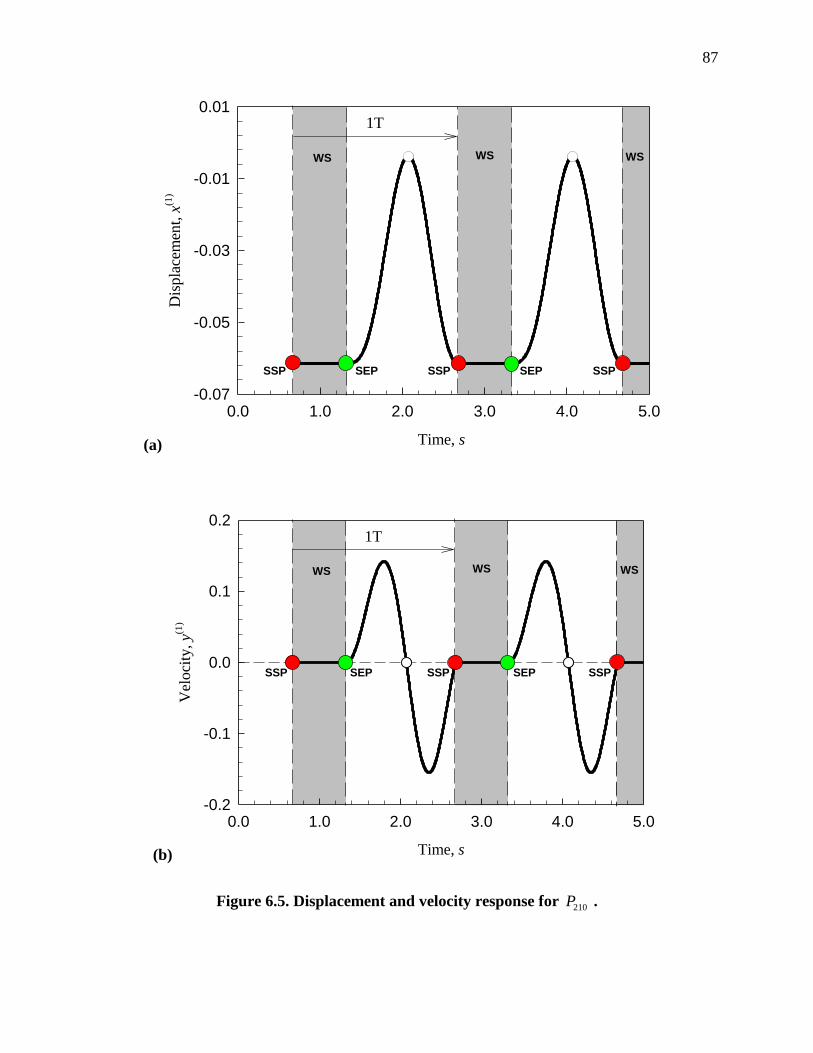
87
(a) Time, s
0.0 1.0 2.0 3.0 4.0 5.0
Dis
pla
cem
ent,
x(1
)
-0.07
-0.05
-0.03
-0.01
0.011T
SSP SSPSEP
WS WS WS
SSP SEP
(b)
1T
SSP SSPSEP
WS WS WS
SSP SEP
Time, s
0.0 1.0 2.0 3.0 4.0 5.0
Vel
oci
ty, y(1
)
-0.2
-0.1
0.0
0.1
0.2
Figure 6.5. Displacement and velocity response for 210P .

88
(a)
1T
SSP
WS WS WS
Time, s
0.0 1.0 2.0 3.0 4.0 5.0
Acc
eler
atio
n, a
(1)
-1.0
-0.5
0.0
0.5
1.0
SEPSSPSEP SSP
(b)Displacement, x
(1)
-0.07 -0.05 -0.03 -0.01 0.01
Vel
oci
ty, y(1
)
-0.2
-0.1
0.0
0.1
0.2
P2
P0
P1
Figure 6.6. Acceleration response and phase plane trajectory for 210P .
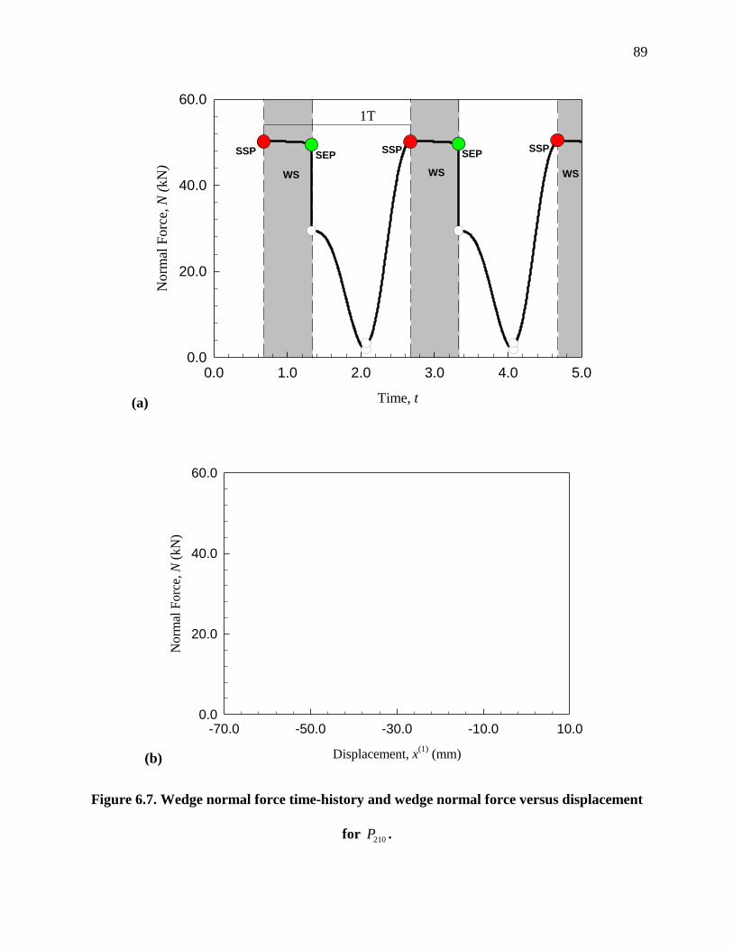
89
(a)
1T
WS WS WS
Time, t
0.0 1.0 2.0 3.0 4.0 5.0
Norm
al F
orc
e, N
(kN
)
0.0
20.0
40.0
60.0
SSPSEP
SSP SEPSSP
(b) Displacement, x(1)
(mm)
-70.0 -50.0 -30.0 -10.0 10.0
Norm
al F
orc
e, N
(kN
)
0.0
20.0
40.0
60.0
Figure 6.7. Wedge normal force time-history and wedge normal force versus displacement
for 210P .
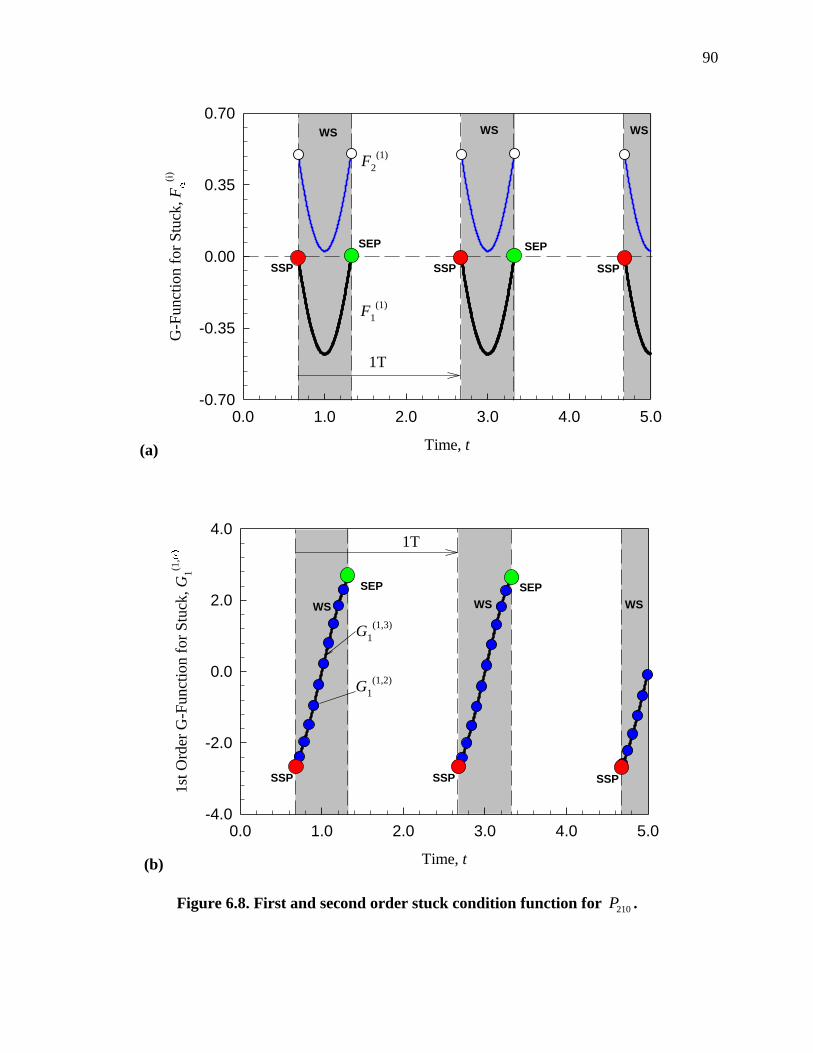
90
(a)
F2
(1)
F1
(1)
1T
SSP
WS WS WS
SEP
SSP
Time, t
0.0 1.0 2.0 3.0 4.0 5.0
G-F
unct
ion f
or
Stu
ck, F
(i)
-0.70
-0.35
0.00
0.35
0.70
SSP
SEP
(b)
G1
(1,2)
G1
(1,3)
WS
Time, t
0.0 1.0 2.0 3.0 4.0 5.0
1st
Ord
er G
-Fu
nct
ion
fo
r S
tuck
, G
1
(1,
-4.0
-2.0
0.0
2.0
4.0
SSP SSPSSP
SEPSEP
WSWS
1T
Figure 6.8. First and second order stuck condition function for 210P .

91
conditions are satisfied. Furthermore, stuck motion for the freight train suspension system may
be catastrophic because there will be no system damping.
6.4 Work Dissipation by Friction
From the analytical prediction of periodic solutions for the entire possible range of wedge
angles, clearly the wedge angle plays a critical role in determining the train suspension response.
From the mapping structure, smaller wedge angles presented the addition of one or more stuck
mappings. Since a smaller wedge angle will transfers more of the normal force between the
wedge and bolster into the side-frame, there is an increasing likelihood of stuck motion. While
the goal of the wedge is to act as a friction damper, there is a trade-off between increasing the
friction damping and causing more stuck motion. Furthermore, stuck motion for the train
suspension system means a temporary loss of suspension. Without an active suspension system, a
train may lose control and derail. On the other hand, a larger wedge angle transfers less normal
force and thus is less likely to endure stuck motion. In fact, with larger wedge angles, the stuck
motion disappears. The trade-off now becomes less or no stuck motion versus reduced damping
capacity. To help quantify the differences in wedge angle performance, the displacement,
acceleration, and work done by friction will be considered for various wedge angles.
From Physics, the work done by a force is given by
( )W F s ds (121)
where ( )F s is the force acting over a known distance. For the force of friction acting on the
wedge and bolster, the work done can be determined by
2
1
( )x
kx
W F x dx (122)
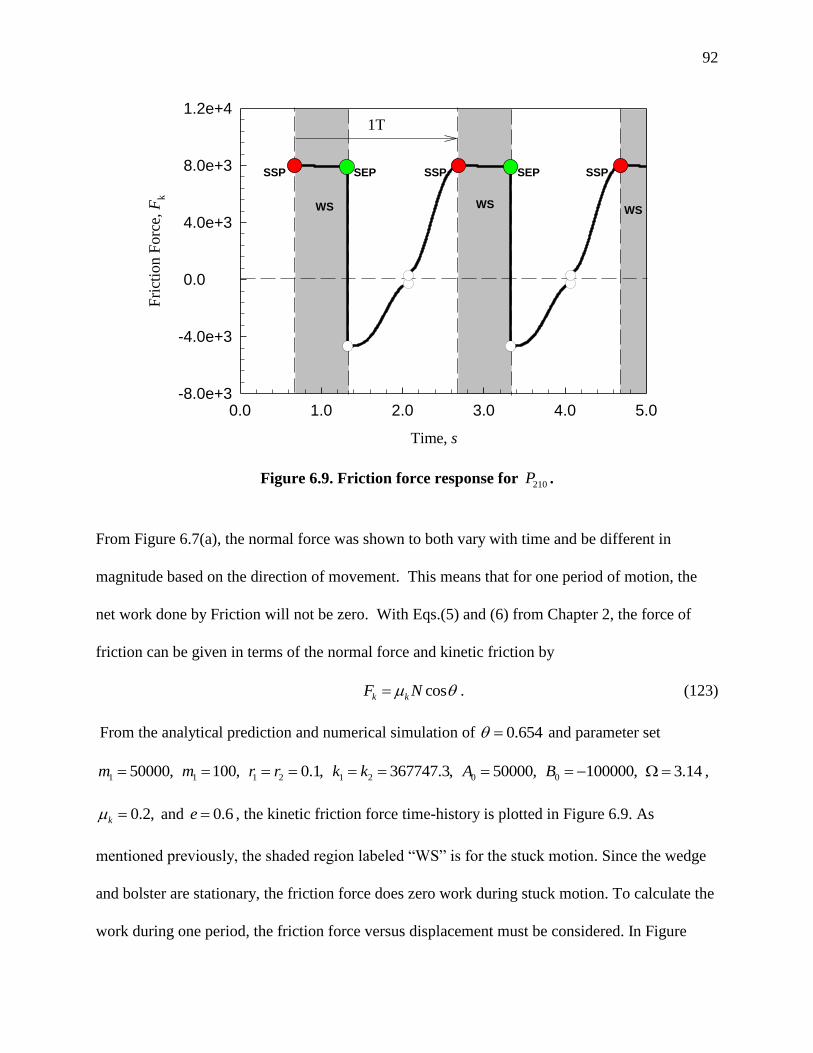
92
1T
SSPSEP SSP SEP
Time, s
0.0 1.0 2.0 3.0 4.0 5.0
Fri
ctio
n F
orc
e, F
k
-8.0e+3
-4.0e+3
0.0
4.0e+3
8.0e+3
1.2e+4
WSWSWS
SSP
Figure 6.9. Friction force response for 210P .
From Figure 6.7(a), the normal force was shown to both vary with time and be different in
magnitude based on the direction of movement. This means that for one period of motion, the
net work done by Friction will not be zero. With Eqs.(5) and (6) from Chapter 2, the force of
friction can be given in terms of the normal force and kinetic friction by
cosk kF N . (123)
From the analytical prediction and numerical simulation of 0.654 and parameter set
1 50000,m 1 100,m 1 2 0.1,r r 1 2 367747.3,k k 0 50000,A 0 100000,B 3.14 ,
0.2,k and 0.6e , the kinetic friction force time-history is plotted in Figure 6.9. As
mentioned previously, the shaded region labeled “WS” is for the stuck motion. Since the wedge
and bolster are stationary, the friction force does zero work during stuck motion. To calculate the
work during one period, the friction force versus displacement must be considered. In Figure

93
6.10, the friction force is plotted for negative and positive velocity, respectively. The area under
the curve denotes the amount of work done by Friction.
Based on the simulation results, the curves in Figures 6.10(a) and (b) were numerically
integrated to give -142.64J and -242.94J for the friction during negative and positive velocity,
respectively. Note, since friction acts in the opposite direction to movement the work will
necessary be negative. Based on the amount of work done, the friction damping is significantly
more effective when the wedge and bolster are moving downward as opposed to upward. This
“wedge effect” is also confirmed by the field testing data provided by Amsted Rail. From Figure
6.2, the normal force is significantly larger with negative velocity, which means that the friction
damping would also be much larger.
To further discuss the wedge angle relationship to suspension performance, additional
wedge angles must be considered. From the analytical prediction, several wedge angle solutions
were simulated to quantify displacement, acceleration and work. In Table 6.2, the results are
tabulated for the sake of brevity and clarity. As the wedge angle is increased, the displacement
range increases slightly while the work done by friction decreases. Notice, for 0.38 and
0.92 the maximum displacement is -0.0542 and -0.0682, respectively. If friction is doing less
work in damping, the displacement of the bolster and wedge will likely increase. On the other
hand, the acceleration is also an important response. With smaller angles the acceleration is
larger, (i.e., -0.7288 and -0.894 for 0.38 and 0.92 , respectively). Slowing the bolster
down over a smaller distance will certainly require higher acceleration and vice versa. The
current wedge angle used by industry is 37.5 or 0.654rad , also described in Table 6.2. As
compared to the larger wedge angle 0.92 , the displacement, acceleration, and work done by
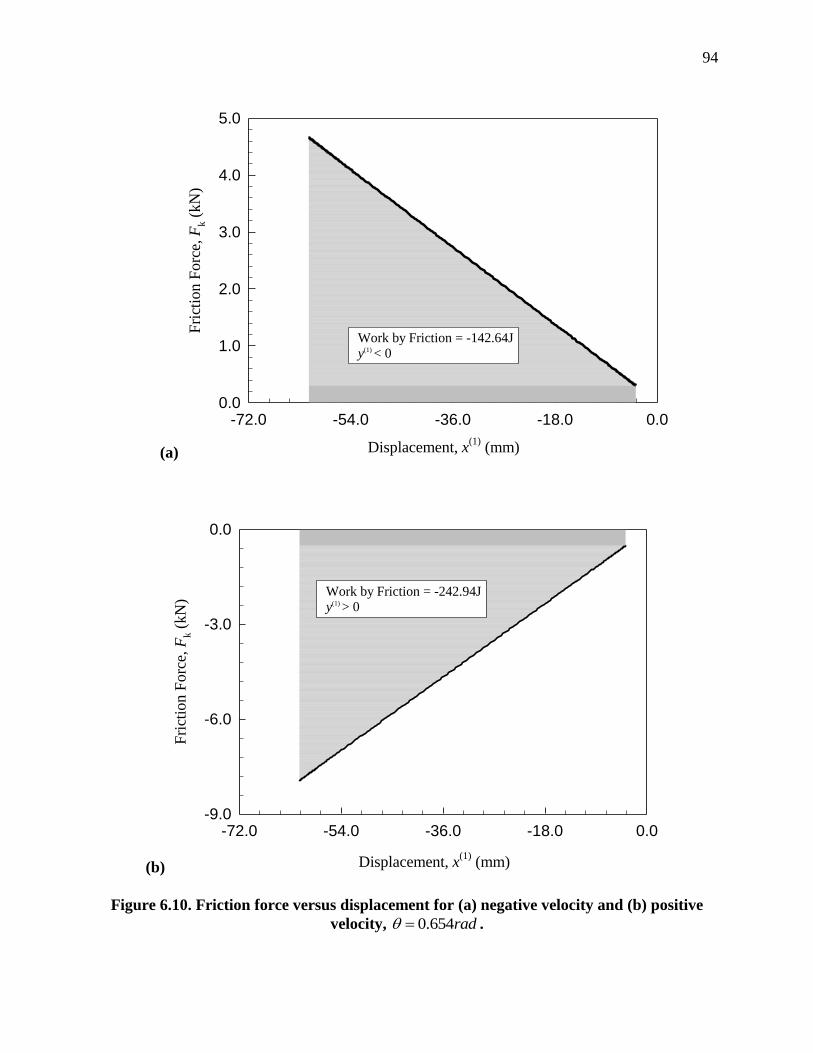
94
(a) Displacement, x(1)
(mm)
-72.0 -54.0 -36.0 -18.0 0.0
Fri
ctio
n F
orc
e, F
k (
kN
)
0.0
1.0
2.0
3.0
4.0
5.0
Work by Friction = -142.64J
y(1) < 0
(b) Displacement, x(1)
(mm)
-72.0 -54.0 -36.0 -18.0 0.0
Fri
ctio
n F
orc
e, F
k (
kN
)
-9.0
-6.0
-3.0
0.0
Work by Friction = -242.94Jy(1) > 0
Figure 6.10. Friction force versus displacement for (a) negative velocity and (b) positive
velocity, 0.654rad .

95
friction are quite similar. The major and most important difference is the mapping structure. By
increasing the wedge angle from 0.654 to 0.92, the wedge and bolster no longer endure stuck
motion at the cost of slightly less friction damping.
Table 6.2. Tabulated values of displacement acceleration and work.
Wedge,
(rad)
Displacement Range
( )m
Acceleration Range 2( )m s
Work by Friction,
( )J
0.38 , 210P (-0.0542,-0.00535) (-0.8941,0.6169) -152.43, -456.88
0.50, 210P (-0.0592,-0.00375) (-0.8953,0.5846) -155.28, -333.07
0.654 , 210P (-0.0614,-0.0542) (-0.8656,-0.0542) -142.64, -242.94
0.92 , 21P (-0.0682,-0.00637) (-0.7288,0.4212) -146.67, -199.06

96
CHAPTER VII
SUMMARY
In this Dissertation, a mechanical model for a freight train suspension system was
developed to include all possible types of motion such as free-flight, stick, and stuck motion.
The dynamic mechanism of the impacting chatter with stick was investigated from the local
singularity theory of discontinuous dynamical systems. The analytical conditions for the onset
and vanishing of stick motions were presented, and the condition for maintaining stick motion
was achieved as well. Due to the possibility of stuck motion, additional analytical conditions
were developed to determine the onset and vanishing conditions for stuck motion. Analytical
prediction of periodic motions relative to impacting chatter with stick and stuck in train
suspension was completed through the mapping structure. The corresponding local stability and
bifurcation analyses were carried out, and the grazing and stick conditions were used for the
existence of periodic motions. Numerical simulations were performed to illustrate the periodic
motions of stick and stuck motion. Finally, based on field testing data, an investigation into the
effects of wedge angle was conducted to find a more desirable suspension response.
In Chapter 1, the mechanical model of a typical freight train suspension system was
presented. The corresponding literature survey about the previous and more current status of
train suspension systems was completed. In Chapter 2, because of the discontinuity between the
wedge and bolster with friction, the domain partition in phase plane was discussed. The
corresponding dynamical system on such sub-domains was presented in the absolute and relative
frames. Further, the mathematical description of the train suspension system was given. In
Chapter 3, the analytical conditions for grazing and stick phenomena, as well as stuck motion,
97
were developed, which included the necessary and sufficient conditions. In Chapter 4, the basic
mappings and switching sets were introduced in the absolute and relative frame. The generalized
mapping structure for periodic motion was presented. In addition, consider generic parameters,
the bifurcation scenario versus excitation frequency was presented. In Chapter 5, the
methodology for analytical prediction of periodic motion was given, and the local stability and
bifurcation conditions were presented. The impacting chatter with stick and stuck were
analytically predicted, and the local stability and bifurcation was given through the eigenvalue
analysis. To help one better understand such mathematical conditions, numerical illustrations of
period motion from the predicted solutions demonstrated the physical interpretation of the stick
and stuck conditions. In Chapter 6, field testing data was considered to obtain a more realistic
parameter set. Based on analytical predictions of periodic motion, the entire range of possible
wedge angles was investigated. Considering the displacement, acceleration, and work done by
friction in damping the system, a comparison study described the benefits of having a larger
wedge angle.
Through this investigation, the motion mechanism of the ubiquitous freight train
suspension system can be further understood, which may provide some clues to reduce the
possibility of poor suspension performance and further derailment. According to industry, a
leading cause for derailment at high speeds is suspension performance. Current investigations
are interested in what industry calls the “slip-stick” phenomena. Here “slip-stick” refers to the
wedge and bolster sticking to the side-wall, otherwise known as “stuck” motion herein. Through
further parameter studies, the mechanical model presented herein can be utilized to recommend
better performing suspension characteristics such as wedge angle, spring stiffness, friction
coefficients, etc.

98
REFERENCES
Chandiramani, N.K., Srinivasan, K. Nagendra, J. (2006). “Experimental study of stick-slip
dynamics in a friction wedge damper”, Journal of Sound and Vibration, 291, pp. 1-18.
Comparin, R.J. and Singh, R. (1989). “Nonlinear frequency response characteristics of an impact
pair,” Journal of Sound and Vibration, 134, pp.259-290.
Feeny, B.F. (1992). “A nonsmooth Coulomb friction oscillator”, Physics D, 59, pp. 25–38.
Gardner, J.F. and Cusumano, J. P. (1997). “Dynamic models of friction wedge dampers”,
Proceedings of the 1997 IEEE/ASME Joint Railroad Conference, Boston, MA, pp. 65-69.
Gottzein, E. and Lange, B. (1975). “Magnetic suspension control systems for the MBB high
speed train”, Automatica, 11, pp.271-284.
Ju, S.-H. and Lin, H.-T. (2008). “Experimentally investigating finite element accuracy for ground
vibrations induced by high-speed trains”, Engineering Structures, 30, pp. 733-746.
Kaiser A. B., Cusumano J. P., and Gardner J. F. (2002). “Modeling and dynamics of friction
wedge dampers in railroad freight trucks”, Vehicle System Dynamics, 38, pp.55-82.
Pfeiffer, F. (1984). “Mechanische Systems mit unstetigen Ubergangen,” Ingeniuer- Archiv, 54,
pp.232-240.
Hinrichs, N., Oestreich, M., and Popp. K. (1997). “Dynamics of oscillators with impact and
friction”, Chaos, Solitons, and Fractals, 8 (4), pp. 535–558.
Hundal, M.S. (1979). “Response of a base excited system with Coulomb and viscous friction”,
Journal of Sound and Vibration, 64, pp. 371–378.
Karagiannis, K. and Pfeiffer, F. (1991). “Theoretical and experimental investigations of gear
box”, Nonlinear Dynamics, 2, pp.367-387.
Karlström, A. B. (2006). “An analytical model for train-induced ground vibrations from
railways”, Journal of Sound and Vibration, 292, pp. 221-241.

99
Luo, A.C.J. (2005). “A theory for non-smooth dynamic systems on the connectable Domains,”
Communications in Nonlinear Science and Numerical Simulation, 10, pp.1-55.
Luo, A.C.J., and Chen, L.D. (2005). “Periodic motion and grazing in a harmonically forced,
piecewise linear, oscillator with impacts,” Chaos, Solitons and Fractals, 24, pp.567-578.
Luo, A.C.J. and Gegg, B.C. (2006). “Stick and non-stick periodic motions in periodically forced
oscillators with dry friction”, Journal of Sound and Vibration, 291, pp.132-168.
Luo, A.C.J. and O’Connor, D.M. (2009). “Mechanism of impacting chatter with stick in a gear
transmission system”, International Journal of Bifurcation and Chaos, 19, pp.2093-2105.
Luo, A.C.J. and O’Connor, D.M. (2009). “Periodic motions and Chaos with Impacting Chatter
and stick in a Gear Transmission System”, International Journal of Bifurcation and
Chaos, 19, pp.1975-1994.
Sayyaadi, H. and Shokouhi, N. (2009). “A new model in rail–vehicles dynamics considering
nonlinear suspension components behavior”, International Journal of Mechanical
Sciences, 51, pp. 222-232.
Shieh, N.-C., Lin, C.-L., Lin, Y.-C. Liang, K.-Z. (2005). “Optimal design for passive suspension
of a light rail vehicle using constrained multiobjective evolutionary search” Journal of
Sound and Vibration, 285, pp. 407-424.
Shaw, S.W. (1986). “On the dynamic response of a system with dry-friction”, Journal of Sound
and Vibration, 108, pp. 305–325.
Shaw, S. W. and Holmes, P.J. (1983). “A Periodically Forced Piecewise Linear Oscillator,”
Journal of Sound and Vibration, 90(1), pp.129-155.
Theodossiades, S. and Natsiavas, S. (2000). “Non-linear dynamics of gear-pair systems with
periodic stiffness and backlash,” Journal of Sound and Vibration, 229(2), pp 287-310.
Wu, Y.-S., and Yang, Y.-B. (2003). “Steady-state response and riding comfort of trains moving
over a series of simply supported bridges”, Engineering Structures, 25, pp. 251-265.

APPENDICES
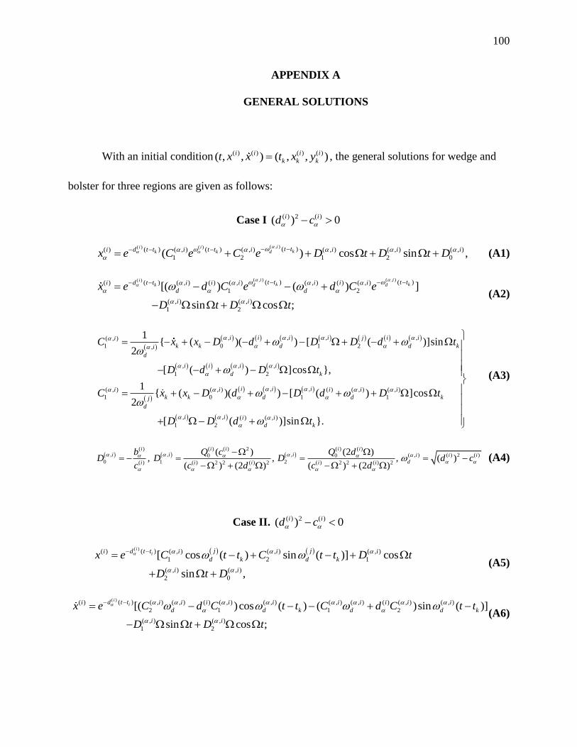
100
APPENDIX A
GENERAL SOLUTIONS
With an initial condition ( ) ( ) ( ) ( )( , , ) ( , , )i i i i
k k kt x x t x y , the general solutions for wedge and
bolster for three regions are given as follows:
Case I ( ) 2 ( )( ) 0i id c
( , )( ) ( ) ( )( ) ( )( ) ( , ) ( , ) ( , ) ( , ) ( , )
1 2 1 2 0( ) cos sin ,ii i
kk k d t td t t t ti i i i i ix e C e C e D t D t D
(A1)
( , ) ( , )( ) ( ) ( )( )( ) ( , ) ( ) ( , ) ( , ) ( ) ( , )
1 2
( , ) ( , )
1 2
[( ) ( ) ]
sin cos ;
i iik kk d dt t t td t ti i i i i i i
d d
i i
x e d C e d C e
D t D t
(A2)
, , , ,( , )
1 0 1 2,
, , ,
1 2
, ,( , ) ( , ) ( ) ( , ) ( , )
1 0 1 1
,
1 2
1{ ( )( ) [ ( )]sin
2
[ ( ) ]cos },
1{ ( )( ) [ ( ) ]cos
2
[
i i i i j i ii
k k d d ki
d
i i i i
d k
i i ii i i i i
k k d d kj
d
i
C x x D d D D d t
D d D t
C x x D d D d D t
D D
, ( ) ( , )( )]sin }.
i i i
d kd t
(A3)
( ) ( ) ( ) 2 ( ) ( )
, , , ( , ) ( ) 2 ( )0 0
0 1 2( ) ( ) 2 2 ( ) 2 ( ) 2 2 ( ) 2
( ) (2 ), , , ( )
( ) (2 ) ( ) (2 )
i i i i ii i i i i i
di i i i i
b Q c Q dD D D d c
c c d c d
(A4)
Case II. ( ) 2 ( )( ) 0i id c
( ) ( )( ) ( , ) ( , ) ( , )
1 2 1
( , ) ( , )
2 0
[ cos ( ) sin ( )] cos
sin ,
ii j jd t ti i i i
d k d k
i i
x e C t t C t t D t
D t D
(A5)
( ) ( )( ) ( , ) ( , ) ( ) ( , ) ( , ) ( , ) ( , ) ( ) ( , ) ( , )
2 1 1 2
( , ) ( , )
1 2
[( )cos ( ) ( )sin ( )]
sin cos ;
iid t ti i i i i i i i i i i
d d k d d k
i i
x e C d C t t C d C t t
D t D t
(A6)
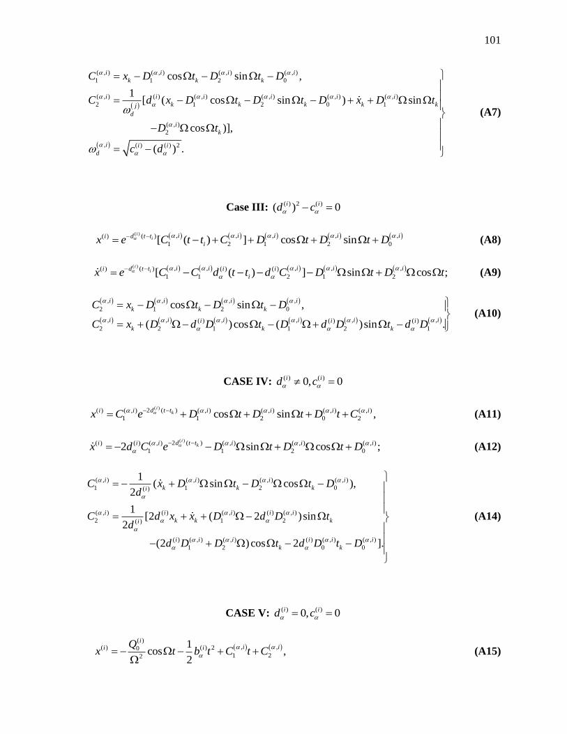
101
( , ) ( , ) ( , ) ( , )
1 1 2 0
( , ) ( ) ( , ) ( , ) ( , ) ( , )
2 1 2 0 1
( , )
2
, ( ) ( ) 2
cos sin ,
1[ ( cos sin ) sin
cos )],
( ) .
i i i i
k k k
i i i i i i
k k k k kj
d
i
k
i i i
d
C x D t D t D
C d x D t D t D x D t
D t
c d
(A7)
Case III: ( ) 2 ( )( ) 0i id c
( ) , , , , ,( )( )
1 2 1 2 0[ ( ) ] cos sini
i i i i i id t ti
ix e C t t C D t D t D (A8)
( ) , , , , ,( )( ) ( ) ( )
1 1 2 1 2[ ( ) ] sin cos ;i
i i i i i id t ti i i
ix e C C d t t d C D t D t
(A9)
, , , ,
2 1 2 0
, , , , , ,( ) ( ) ( )
2 2 1 1 2 1
cos sin ,
( )cos ( )sin .
i i i i
k k k
i i i i i ii i i
k k k
C x D t D t D
C x D d D t D d D t d D
(A10)
CASE IV: ( ) ( )0, 0i id c
( )2 ( )( ) ( , ) ( , ) ( , ) ( , ) ( , )
1 1 2 0 2cos sin ,i
kd t ti i i i i ix C e D t D t D t C (A11)
( )2 ( )( ) ( ) ( , ) ( , ) ( , ) ( , )
1 1 2 02 sin cos ;i
kd t ti i i i i ix d C e D t D t D
(A12)
( , ) ( , ) ( , ) ( , )
1 1 2 0( )
( , ) ( ) ( , ) ( ) ( , )
2 1 2( )
( ) ( , ) ( , ) ( ) ( , ) ( , )
1 2 0 0
1( sin cos ),
2
1[2 ( 2 )sin
2
(2 )cos 2 ].
i i i i
k k ki
i i i i i
k k ki
i i i i i i
k k
C x D t D t Dd
C d x x D d D td
d D D t d D t D
(A14)
CASE V: ( ) ( )0, 0i id c
( )
, ,( ) ( ) 201 22
1cos ,
2
ii ii iQ
x t b t C t C
(A15)

102
( )
,( ) ( )01sin ;
iii iQ
x t b t C
(A16)
( ), ( )0
1
( ) ( ), ( ) 20 0
2 2
sin ,
1cos sin .
2
ii i
k k k
i ii i
k k k k k k
QC x t b t
Q QC x xt t t t b t
(A17)

103
APPENDIX B
NUMERICAL SIMULATION ALGORITHM
The numerical simulation algorithm used in this thesis is for plotting the displacement
and velocity response of each oscillator in the mechanical model in Fig.2. For the equations of
motion in Eqs.(1) and (7), the closed form solutions and their corresponding homogeneous
coefficients (i.e., displacement and velocity equations) can be found in Appendix A. These
equations are programmed in C++. Additionally, the impact relationship in Eq.(4) as well as the
analytical conditions for stick onset and vanishing are programmed. Assuming that the
oscillators are described by Eq.(1) with initial conditions ( ) ( ) ( )( , , , )i i i
k k k kt x x x and by incrementing
time by a small amount kt , the new displacement and velocity of each mass can be computed
for the new time. After each increment, the conditions for impact are checked. Once impact
occurs at the boundary, the initial conditions ( ) ( ) ( )( , , , )i i i
k k k kt x x x are updated. If the stick
conditions are satisfied, then the two oscillators are described by Eq.(7). While in stick motion,
the wedge and bolster may become stuck when crossing the velocity boundary. If the analytical
conditions for stuck are satisfied, the oscillators will become fixed to the side frame. This
process of incrementing time, computing displacements and velocities, checking impact and stick
conditions, and updating the initial conditions to be those at the domain boundaries is repeated
until the motion can be considered either periodic or chaotic. By keeping track of the switching
boundaries, the mapping structure can be defined and a bifurcation scenario presented as shown
in Chapter 4. Furthermore, by recording all the computations at each time step, the motion can
be numerically simulated as shown in Chapter 5.
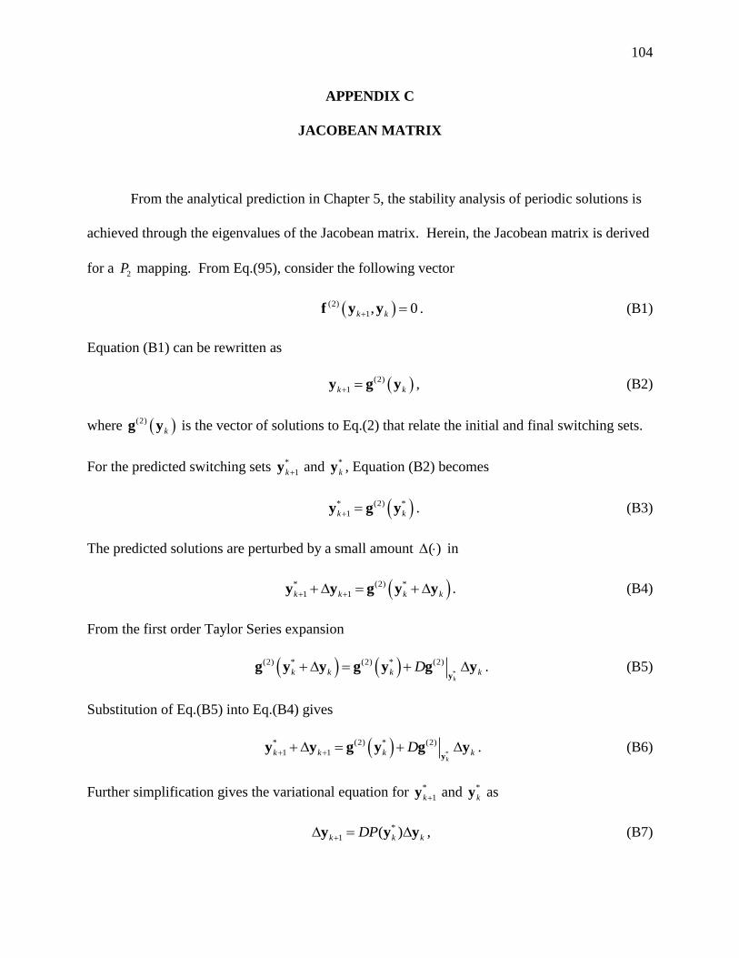
104
APPENDIX C
JACOBEAN MATRIX
From the analytical prediction in Chapter 5, the stability analysis of periodic solutions is
achieved through the eigenvalues of the Jacobean matrix. Herein, the Jacobean matrix is derived
for a 2P mapping. From Eq.(95), consider the following vector
(2)
1, 0f y yk k . (B1)
Equation (B1) can be rewritten as
(2)
1y g yk k , (B2)
where (2)g yk is the vector of solutions to Eq.(2) that relate the initial and final switching sets.
For the predicted switching sets *
1yk and *y k , Equation (B2) becomes
* (2) *
1y g yk k . (B3)
The predicted solutions are perturbed by a small amount ( ) in
* (2) *
1 1y y g y yk k k k . (B4)
From the first order Taylor Series expansion
*
(2) * (2) * (2)
yg y y g y g y
kk k k kD . (B5)
Substitution of Eq.(B5) into Eq.(B4) gives
*
* (2) * (2)
1 1 yy y g y g y
kk k k kD . (B6)
Further simplification gives the variational equation for *
1yk and *y k as
*
1 ( )y y yk k kDP , (B7)

105
where the Jacobean Matrix *
(2)
yg
k
D is represented by *( )ykDP . The total derivatives of the
displacement and velocity functions represented in Eq.(B1) provide the components of DP .
(1) (1) (2)(2) (2) (2) (2) (2)
1 1 1 11 1 1 1 1
(1) (1) (2)
1 1 1 1
(1) (1)(2) (2) (2) (2)
1 1 11 1 1 1
(1) (1) (1) (1) (1) (
1 1 1
0k k k k
k k k k k k k k k
k k k
k k k k k k k
t x y yf f f f f
t t t x t y t y t
t x yf f f f
x t x x x y x
(2)(2)
11
1) (2) (1)
1
(1) (1) (2)(2) (2) (2) (2) (2)
1 1 1 11 1 1 1 1
(1) (1) (1) (1) (1) (1) (2) (1)
1 1 1 1
(2) (2) (2)
11 1 1
2 (2)
1
0
0
k
k k
k k i k
k k k k k k k k k
k
k k k
yf
y x
t x y xf f f f f
y t y x y y y y y
tf f f
y t y x
(1) (1) (2)(2) (2)
1 1 11 1
(1) (2) (1) (2) (2) (2)
1 1 1
0k k k
k k k k k k
x y yf f
y y y y y
, (B8)
(1) (1) (2)(2) (2) (2) (2) (2)
1 1 1 12 2 2 2 2
(1) (1) (2)
1 1 1 1
(1) (1)(2) (2) (2) (2)
1 1 12 2 2 2
(1) (1) (1) (1) (1) (
1 1 1
0k k k k
k k k k k k k k k
k k k
k k k k k k k
t x y yf f f f f
t t t x t y t y t
t x yf f f f
x t x x x y x
(2)(2)
12
1) (2) (1)
1
(1) (1) (2)(2) (2) (2) (2) (2)
1 1 1 12 2 2 2 2
(1) (1) (1) (1) (1) (1) (2) (1)
1 1 1 1
(2) (2) (2)
12 2 2
2 (2)
1
0
0
k
k k
k k i k
k k k k k k k k k
k
k k k
yf
y x
t x y xf f f f f
y t y x y y y y y
tf f f
y t y x
(1) (1) (2)(2) (2)
1 1 12 2
(1) (2) (1) (2) (2) (2)
1 1 1
0k k k
k k k k k k
x y yf f
y y y y y
, (B9)
(2) (2) (2) (1) (2) (1) (2) (2)
3 3 1 3 1 3 1 3 1
(1) (1) (2)
1 1 1 1
(2) (2) (2) (1) (2) (1)
3 3 1 3 1 3 1
(1) (1) (1) (1) (1) (
1 1 1
0k k k k
k k k k k k k k k
k k k
k k k k k k k
f f t f x f y f y
t t t x t y t y t
f f t f x f y
x t x x x y x
(2) (2)
3 1
1) (2) (1)
1
(2) (2) (2) (1) (2) (1) (2) (2)
3 3 1 3 1 3 1 3 1
(1) (1) (1) (1) (1) (1) (2) (1)
1 1 1 1
(2) (2) (2)
3 3 1 3
2 (2)
1
0
0
k
k k
k k i k
k k k k k k k k k
k
k k k
f y
y x
f f t f x f y f x
y t y x y y y y y
f f t f
y t y x
(1) (2) (1) (2) (2)
1 3 1 3 1
(1) (2) (1) (2) (2) (2)
1 1 1
0k k k
k k k k k k
x f y f y
y y y y y
, (B10)

106
(1) (1) (2)(2) (2) (2) (2) (2)
1 1 1 14 4 4 4 4
(1) (1) (2)
1 1 1 1
(1) (1)(2) (2) (2) (2)
1 1 14 4 4 4
(1) (1) (1) (1) (1) (
1 1 1
0k k k k
k k k k k k k k k
k k k
k k k k k k k
t x y yf f f f f
t t t x t y t y t
t x yf f f f
x t x x x y x
(2)(2)
14
1) (2) (1)
1
(1) (1) (2)(2) (2) (2) (2) (2)
1 1 1 14 4 4 4 4
(1) (1) (1) (1) (1) (1) (2) (1)
1 1 1 1
(2) (2) (2)
14 4 4
2 (2)
1
0
0
k
k k
k k i k
k k k k k k k k k
k
k k k
yf
y x
t x y xf f f f f
y t y x y y y y y
tf f f
y t y x
(1) (1) (2)(2) (2)
1 1 14 4
(1) (2) (1) (2) (2) (2)
1 1 1
0k k k
k k k k k k
x y yf f
y y y y y
. (B11)
The partial derivatives of the final time, position, and velocities in Eqs.(B8)-(B11) are the
necessary derivatives for Jacobean matrix DP in Eq.(108). These derivatives can be found by
arranging the functions in matrix form (i.e., solve four systems of four equations each with four
unknowns).
(2)1 1
(1) (2)1 2
1
(1) (2)1 3
(2) (2)1 4
k
k k
k
i k
k
k k
k
k k
t f
t t
x f
t t
y f
t t
y f
t t
,
(2)1 1
(1) (1)
(1) (2)1 2
(1) (1)1
(1) (2)1 3
(1) (1)
(2) (2)1 4
(1) (1)
k
k k
k
k k
k
k k
k
k k
t f
x x
x f
x x
y f
x x
y f
x x
, (B12)
(2)1 1
(1) (1)
(1) (2)1 2
(1) (1)1
(1) (2)1 3
(1) (1)
(2) (2)1 4
(1) (1)
k
k k
k
k k
k
k k
k
k k
t f
y y
x f
y y
y f
y y
y f
y y
,
(2)1 1
(2) (2)
(1) (2)1 2
(2) (2)1
(1) (2)1 3
(2) (2)
(2) (2)1 4
(2) (2)
k
k k
k
k k
k
k k
k
k k
t f
y y
x f
y y
y f
y y
y f
y y
. (B13)
The Lambda matrix is defined by

107
(2) (2) (2) (2)
1 1 1 1
(1) (1) (2)
1 1 1 1
(2) (2) (2) (2)
2 2 2 2
(1) (1) (2)
1 1 1 1
(2) (2) (2) (2)
3 3 3 3
(1) (1) (2)
1 1 1 1
(2) (2) (2)
4 4 4
(1) (1)
1 1 1
k k k i
k k k k
k k k k
k k k
f f f f
t x y y
f f f f
t x y y
f f f f
t x y y
f f f
t x y
(2)
4
(2)
1k
f
y
. (B14)
After solving each system of equations in Eqs.(B12) and (B13), the derivatives for the Jacobean
matrix are known and the first 2DP matrix of Eq.(107) can be given. The above process is
repeated for each subsequent mapping.

108
VITA
Graduate School
Southern Illinois University
Dennis O’Connor
Southern Illinois University Edwardsville
Bachelor of Science, Mechanical Engineering, May 2004
Southern Illinois University Edwardsville
Master of Science, Mechanical Engineering, May 2007
Dissertation Title:
ON MOTION MECHANISMS IN FREIGHT TRAIN SUSPENSION SYSTEMS
Major Professor: Albert C.J. Luo
Publications:
Journal Articles
1. Luo, Albert C.J. and Dennis O’Connor (2014), “On periodic motions in a parametric hardening
Duffing oscillator”, International Journal of Bifurcation and Chaos, 24, 1430004.
2. Luo, Albert C.J. and Dennis O’Connor (2009), “Periodic Motions with Impacting Chatter and
Stick in a Gear Transmission System”, ASME Journal of Vibration and Acoustics, 131, 041013
3. Luo, Albert C.J. and Dennis O’Connor (2009), “Impact Chatter in a gear transmission system with
two oscillators”, IMeChe Part K: Journal of Multi-body Dynamics, 223, 159-188.
4. Luo, Albert C.J. and Dennis O’Connor (2009), “Mechanism of impacting chatter with stick in a
gear transmission system”, International Journal of Bifurcation and Chaos, 19, 1975-1994
5. Luo, Albert C.J. and Dennis O’Connor (2009), “Periodic motions and chaos with impacting
chatter with stick in a gear transmission system”, International Journal of Bifurcation and Chaos,
19, 2093-2105.
Conference Papers
1. Luo, Albert C. J. and Dennis O’Connor, “Analytical Solutions for periodic motions in a
Hard-ening Mathieu-Duffing oscillator”, in 2013 ASME San Diego, California, USA
2. Luo, Albert C. J. and Dennis O’Connor, “Coexisting Asymmetric and Symmetric
Periodic Mo-tions in the Mathieu-Duffing Oscillator”, in 2012 ASME International
Mechanical Engineering Congress and Exposition, Houston, Texas, November 9-15,
2012. IMECE2012-86849.

109
3. Luo, A.C.J. and Dennis O’Connor, “Stable and Unstable Periodic Solutions to Mathiu-
Duffing Oscillator”, Proceedings of IEEE 4th Conference on Nonlinear Science and
Complexity, Bu-dapest, Hungary, August 6-11, 2012. pp.201-204.
4. Luo, Albert C. J. and Dennis O’Connor, “Analytical Dynamics of Complex Motions in a
Train Suspension System”, in 2011 ASME International Mechanical Engineering
Congress and Ex-position, Denver, Colorado, November 11-17, 2011. IMECE2011-
62944.
5. Luo, Albert C. J. and Dennis O’Connor, “Dynamic mechanism of a train suspension
system”, in 2010 ASME International Mechanical Engineering Congress and Exposition,
Vancouver, British Columbia, November 12-18, 2010. IMECE2010-39202.
6. Luo, Albert C.J. and Dennis O’Connor, “Periodic and chaotic motions in a gear-pair
transmis-sion systems with impacts”, The second International Conference on Nonlinear
Science and Complexity, Porto, Portugal, July 26-31, 2008.
7. Luo, Albert C.J. and Dennis O’Connor, “Nonlinear dynamics of a gear transmission
system: Part I: Mechanism of impact chatters with stick”, 2007 ASME International
Design Engineer-ing Technical Conference


![TLI42615 Certificate IV in Train Driving [Freight]€¦ · · 2016-04-18TLI42615 Certificate IV in Train Driving [Freight] T Railtrain deliver and assess TLI42615 Certificate IV](https://static.fdocuments.us/doc/165x107/5af7fd5a7f8b9ae94890db51/tli42615-certificate-iv-in-train-driving-freight-2016-04-18tli42615-certificate.jpg)