On-line Bayesian Context Change Detection in WebService Systems

Maciej Zięba, Jakub M. Tomczak

HotTopiCS 2013

maciej.zieba@spwr.wroc.pl

Prague, 20.04.2013

Agenda

1. Problem background

2. Change detection problem statement

3. Approaches for solving the problem

4. Bayesian Model

5. Algorithm for change detection

6. Simulation environment

7. Results and discussion

2/23

Problem backgroundSOA-based systems

SOA-based systems: systemsthat implement ServiceOriented Architecture, i.e., anarchitectural style whose goal isto achieve loose couplingamong interacting softwarecomponents called services.

SOA-based systems

Services Execution system

3/23

Problem backgroundSOA-based systems

SOA-based systems: systemsthat implement ServiceOriented Architecture, i.e., anarchitectural style whose goal isto achieve loose couplingamong interacting softwarecomponents called services.

Services: self-describing,stateless, modular applicationsthat are distributed across theWeb and which providefunctionalities and are describedby quality attributes (QoS).

SOA-based systems

Services Execution system

3/23

Problem backgroundSOA-based systems

SOA-based systems: systemsthat implement ServiceOriented Architecture, i.e., anarchitectural style whose goal isto achieve loose couplingamong interacting softwarecomponents called services.

Execution system: network of virtual machines; distributed computational

resources; input: streams of requests; output: system performance,

e.g., latency.

SOA-based systems

Services Execution system

3/23

Problem backgroundResource allocation problem

In order to maintain theperformance of an executionsystem at a satisfactory (orgiven) level the followingdecisions are mainly be made:

migration of services;

computational resourcesallocation.

4/23

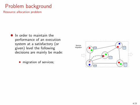
Problem backgroundResource allocation problem

In order to maintain theperformance of an executionsystem at a satisfactory (orgiven) level the followingdecisions are mainly be made:

migration of services;

computational resourcesallocation.

Service migration

4/23

Problem backgroundResource allocation problem

In order to maintain theperformance of an executionsystem at a satisfactory (orgiven) level the followingdecisions are mainly be made:

migration of services;

computational resourcesallocation.

??

?

??

Resources

4/23

Problem backgroundResource re-allocation

The execution system evolves in time because of:

B non-stationary streams of requests;

B failures or system’s modifications.

Hence, there is a need to propose an adaptive approach forresource allocation.

Resource re-allocation: if a change in the input (or output) isreported, then calculate new resource allocation.

5/23

Problem backgroundResource re-allocation

The execution system evolves in time because of:

B non-stationary streams of requests;

B failures or system’s modifications.

n n+1 n+2

Hence, there is a need to propose an adaptive approach forresource allocation.

Resource re-allocation: if a change in the input (or output) isreported, then calculate new resource allocation.

5/23

Problem backgroundResource re-allocation

The execution system evolves in time because of:

B non-stationary streams of requests;

B failures or system’s modifications.

n n+1 n+2 Failure

Hence, there is a need to propose an adaptive approach forresource allocation.

Resource re-allocation: if a change in the input (or output) isreported, then calculate new resource allocation.

5/23

Problem backgroundResource re-allocation

The execution system evolves in time because of:

B non-stationary streams of requests;

B failures or system’s modifications.

n n+1 n+2 Failure

Hence, there is a need to propose an adaptive approach forresource allocation.

Resource re-allocation: if a change in the input (or output) isreported, then calculate new resource allocation.

5/23

Problem backgroundResource re-allocation

The execution system evolves in time because of:

B non-stationary streams of requests;

B failures or system’s modifications.

n n+1 n+2 Failure

Hence, there is a need to propose an adaptive approach forresource allocation.

Resource re-allocation: if a change in the input (or output) isreported, then calculate new resource allocation.

5/23

Change detection problemOverview

Change detection: identifieschanges in the probabilitydistribution of a stochasticprocess.

Two kinds of changes:

gradual; abrupt.

Statistical change detection: frequentist approach:

distribution estimation andcomparison usingdissimilarity measures;

Bayesian approach: allquantities are randomvariables.

6/23

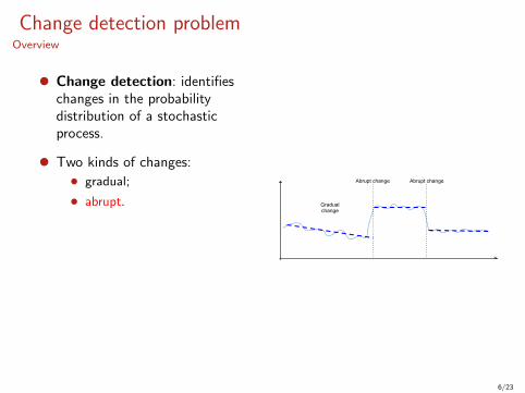
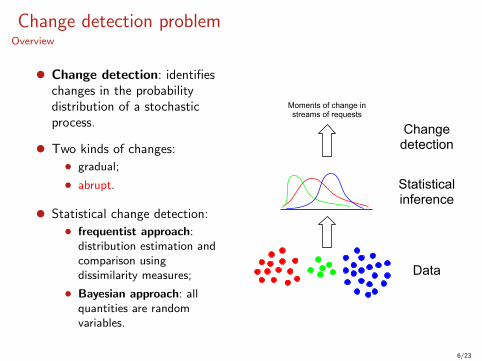
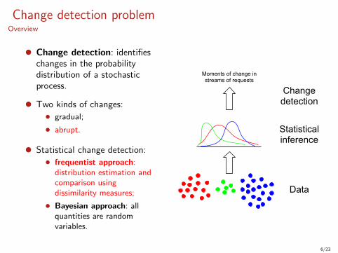
Change detection problemOverview

Change detection: identifieschanges in the probabilitydistribution of a stochasticprocess.

Two kinds of changes:

gradual; abrupt.

Statistical change detection: frequentist approach:

distribution estimation andcomparison usingdissimilarity measures;

Bayesian approach: allquantities are randomvariables.

6/23

Change detection problemOverview

Change detection: identifieschanges in the probabilitydistribution of a stochasticprocess.

Two kinds of changes: gradual;

abrupt.

Statistical change detection: frequentist approach:

distribution estimation andcomparison usingdissimilarity measures;

Bayesian approach: allquantities are randomvariables.

Gradual change

6/23

Change detection problemOverview

Change detection: identifieschanges in the probabilitydistribution of a stochasticprocess.

Two kinds of changes: gradual; abrupt.

Statistical change detection: frequentist approach:

distribution estimation andcomparison usingdissimilarity measures;

Bayesian approach: allquantities are randomvariables.

Gradual change

Abrupt change Abrupt change

6/23

Change detection problemOverview

Change detection: identifieschanges in the probabilitydistribution of a stochasticprocess.

Two kinds of changes: gradual; abrupt.

Statistical change detection: frequentist approach:

distribution estimation andcomparison usingdissimilarity measures;

Bayesian approach: allquantities are randomvariables.

Gradual change

Abrupt change Abrupt change

6/23

Change detection problemOverview

Change detection: identifieschanges in the probabilitydistribution of a stochasticprocess.

Two kinds of changes: gradual; abrupt.

Statistical change detection: frequentist approach:

distribution estimation andcomparison usingdissimilarity measures;

Bayesian approach: allquantities are randomvariables.

Statistical inference

Change detection

Data

Moments of change in streams of requests

6/23

Change detection problemOverview

Change detection: identifieschanges in the probabilitydistribution of a stochasticprocess.

Two kinds of changes: gradual; abrupt.

Statistical change detection: frequentist approach:

distribution estimation andcomparison usingdissimilarity measures;

Bayesian approach: allquantities are randomvariables.

Statistical inference

Change detection

Data

Moments of change in streams of requests

6/23

Frequentist approach

Time

Estimation Estimation

Shifting window 1 Shifting window 2

Dissimilarity measure

7/23

Change detection problemOverview

Change detection: tries toidentify changes in theprobability distribution of astochastic process.

Two kinds of changes: gradual; abrupt.

Statistical change detection: frequentist approach:

distribution estimation andcomparison usingdissimilarity measures;

Bayesian approach: allquantities are randomvariables.

Statistical inference

Change detection

Data

Moments of change in streams of requests

8/23

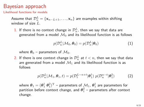
Bayesian approachLikelihood functions for models

Assume that DLn = {xn−L+1, . . . ,xn} are examples within shiftingwindow of size L.

1. If there is no context change in DLn , then we say that data aregenerated from a model M0 and its likelihood function is as follows

p(DLn |M0,θ0) = p(DLn |θ0) (1)

where θ0 – parameters of M0.2. If there is one context change in DLn at t < n, then we say that data

are generated from a model M1 and its likelihood function is asfollows

p(DLn |M1,θ1, t) = p(DL−n+tt |θ11) p(Dn−tn |θ21) (2)

where θ1 = (θ11 θ21)T – parameters of M1, θ11 are parameters for

partition before context change, and θ21 – parameters after contextchange.

9/23

Bayesian approachLikelihood functions for models

Assume that DLn = {xn−L+1, . . . ,xn} are examples within shiftingwindow of size L.

1. If there is no context change in DLn , then we say that data aregenerated from a model M0 and its likelihood function is as follows

p(DLn |M0,θ0) = p(DLn |θ0) (1)

where θ0 – parameters of M0.

2. If there is one context change in DLn at t < n, then we say that dataare generated from a model M1 and its likelihood function is asfollows

p(DLn |M1,θ1, t) = p(DL−n+tt |θ11) p(Dn−tn |θ21) (2)

where θ1 = (θ11 θ21)T – parameters of M1, θ11 are parameters for

partition before context change, and θ21 – parameters after contextchange.

9/23

Bayesian approachLikelihood functions for models

Assume that DLn = {xn−L+1, . . . ,xn} are examples within shiftingwindow of size L.

1. If there is no context change in DLn , then we say that data aregenerated from a model M0 and its likelihood function is as follows

p(DLn |M0,θ0) = p(DLn |θ0) (1)

where θ0 – parameters of M0.2. If there is one context change in DLn at t < n, then we say that data

are generated from a model M1 and its likelihood function is asfollows

p(DLn |M1,θ1, t) = p(DL−n+tt |θ11) p(Dn−tn |θ21) (2)

where θ1 = (θ11 θ21)T – parameters of M1, θ11 are parameters for

partition before context change, and θ21 – parameters after contextchange.

9/23

Bayesian approachModel evidence

In order to select one model which is more probable to generate observeddata we need to calculate model evidences. The model evidence of M0can be calculated as follows

10/23

Bayesian approachModel evidence

In order to select one model which is more probable to generate observeddata we need to calculate model evidences. The model evidence of M0can be calculated as follows

p(DLn |M0) =∫p(DLn |M0,θ0) p(θ0|M0) dθ0, (3)

where p(θ0|M0) – a priori probability distribution of parameters.

10/23

Bayesian approachModel evidence

In order to select one model which is more probable to generate observeddata we need to calculate model evidences. The model evidence of M0can be calculated as follows

p(DLn |M0) =∫p(DLn |M0,θ0) p(θ0|M0) dθ0, (3)

where p(θ0|M0) – a priori probability distribution of parameters. Next,the model evidence of M1 is the following (using the independence ofθ11,θ

21, t)

p(DLn |M1) =x

p(DLn |M1,θ1, t) p(θ11|M1)×

× p(θ21|M1) p(t|M1) dθ1 dt, (4)

where p(θ11|M1), p(θ21|M1), p(t|M1) – a priori probability distributions

of parameters.

10/23

Bayesian approachModel evidence approximation

In order to calculate model evidences of M0 and M1 we make thefollowing assumptions:

the a priori probability distributions of θ0 and θ1 are taken to benon-informative;

the context change occurs in the middle of the shifting window, i.e.,n− d 12Le, hence the a priori probability distribution of t is a Diracdelta function in the point n− d 12Le.

11/23

Bayesian approachModel evidence approximation

In order to calculate model evidences of M0 and M1 we make thefollowing assumptions: the a priori probability distributions of θ0 and θ1 are taken to be

non-informative;

the context change occurs in the middle of the shifting window, i.e.,n− d 12Le, hence the a priori probability distribution of t is a Diracdelta function in the point n− d 12Le.

11/23

Bayesian approachModel evidence approximation

In order to calculate model evidences of M0 and M1 we make thefollowing assumptions: the a priori probability distributions of θ0 and θ1 are taken to be

non-informative; the context change occurs in the middle of the shifting window, i.e.,n− d 12Le, hence the a priori probability distribution of t is a Diracdelta function in the point n− d 12Le.

11/23

Bayesian approachModel evidence approximation

In order to calculate model evidences of M0 and M1 we make thefollowing assumptions: the a priori probability distributions of θ0 and θ1 are taken to be

non-informative; the context change occurs in the middle of the shifting window, i.e.,n− d 12Le, hence the a priori probability distribution of t is a Diracdelta function in the point n− d 12Le.

For such assumptions we can approximate the model evidence by theBayesian Information Criterion (BIC)

ln p(DLn |M) ≈ ln p(DLn |θ̂)−K

2lnL, (5)

where θ̂ is the maximum likelihood estimator of θ.

11/23

Bayesian approachBayes factor

To compare both models, we calculate the Bayes factor (assuming equalprobabilities over models):

B10 =p(DLn |M1)p(DLn |M0)

. (6)

B10 ln(B10) Evidence in favor of M11− 3 0− 1.1 Weak3− 10 1.1− 2.3 Substantial10− 100 2.3− 4.6 Strong> 100 > 4.6 Decisive

12/23

Algorithm descriptionApproximate Bayesian Model Comparison for Change Detection in Web Service Systems 5

and

ln p(DLn |M0) ⇡

KX

k=1

(j1k ln ✓̂1

1,k +j2k ln ✓̂2

1,k)�K ln L. (16)

Finally, we can the approximation of the Bayes fac-tor (13) using (15) and (16), i.e.,

ln B10 ⇡KX

k=1

(j1k ln ✓̂1

1,k+j2k ln ✓̂2

1,k)�KX

k=1

jk ln ✓̂0,k�K

2ln L.

(17)

2.4 Change detection algorithm

Having an analytic form of the approximated Bayes fac-

tor we are able to select one of the two considered mod-els, i.e., one with no context change and the other withone context change. In other words, the selected model

indicate if the context changed occurred in the shift-ing window DL

n or not. Therefore, we can propose anon-line algorithm for change detection. The idea is as

follows. Move shifting window, next calculate the modelevidences (15) and (16) using DL

n . Then calculate theapproximated Bayes factor using (17). The final stepis to report the context change if the Bayes factor is

greater than a given value � 2 R+ called a sensitiv-ity parameter. If the value of the sensitivity parameteris greater, the stronger evidence we want to select the

model M1. In other words, the value of � denotes thesensitivity to the value of the Bayes factor. However,the determination of the � plays a crucial role in theproposed approach and may be seen as [14]:

”(...) a compromise between detecting true changesand avoiding false alarms.”

Nevertheless, we can use the Je↵rey’s interpretation todetermine the value of the sensitivity parameter (see

Table 1).

Let us denote a sequence of context change detec-

tions by ⌧ , and d·e – a ceil function. The final procedureof the change detection is presented in Algorithm 2.

Remarks to Algorithm 2:

1. If N < L, then we take all observations from n = 1to L.

2. If a change is detected, then no further change isreported till the shifting window does not contain

the (N � dL/2e)th observation (lines 6–11).3. Because of the assumptions, the true context change

is in the middle of the shifting window, N � dL/2e.4. The proposed algorithm works as long as new ob-

servations arrive (line 2).

Algorithm 1: Change detection using approxi-mated Bayes factor

Input : D, L, M0, M1

Output: Moments of context change ⌧1, . . . , ⌧M

1 n � 1, m � 0, ⌧0 � 0;2 while n < card{D} do3 Calculate ln p(DL

n |M0) and ln p(DLn |M1) ;

4 Calculate ln B10;5 if ln B10 > � then6 if

�(n� dL/2e)� ⌧m

�> dL/2e then

7 m := m + 1;8 ⌧m � n� dL/2e;9 end

10 end11 n := n + 1;

12 end

Algorithm 2: Change detection using approxi-mated Bayes factor

Input : D, L, M0, M1, �, m := 1, ⌧1 := 1Output: Moments of context change ⌧1, . . . , ⌧M

1 n � 1, m � 0, ⌧0 � 0;2 while n < card{D} do

3 ln p(DLn |M0) �P

k jk ln ✓̂0,k � K2

ln L;

4 ln p(DLn |M1) �P

k(j1k ln ✓̂11,k + j2k ln ✓̂21,k)�K ln L;

5 ln B10 � ln p(DLn |M1)� ln p(DL

n |M0);6 if ln B10 > � then7 if

�(n� dL/2e)� ⌧m

�> dL/2e then

8 m := m + 1;9 ⌧m � n� dL/2e;

10 end

11 end

12 end

5. The computational complexity of Algorithm 2 is

proportional to the size of the shifting window, i.e.,O(L). In order to calculate the model evidences weneed to have the numbers of occurrences of xk whichrequire to read all values of L observations in the

shifting window once only.

3 Experiments

The purpose of this experiment is examine the qual-ity of change detection algorithms which use frequentist

and Bayesian models. We take under consideration webservice execution environment and average latency ofservices’ responses in the system as a time characteristicused for change detection. To reflect the nature of real

web service execution system we propose simulationmodel designed in discrete events simulation environ-ment Arena [3]. The simplified simulation model is pre-

sented in Fig. 2. The model consists of following com-ponents: (i) request generator, which imitates client’s

13/23

SimulatorStructure

&RPSXWDWLRQDO�XQLW

9LUWXDO�PDFKLQH

:HE�VHUYLFH

:HE�VHUYLFH

9LUWXDO�PDFKLQH

:HE�VHUYLFH

:HE�VHUYLFH

5HTXHVW�JHQHUDWRU 6FKHGXOHU 6LQN

&RPSXWDWLRQDO�XQLW

&RPSXWDWLRQDO�XQLW

14/23

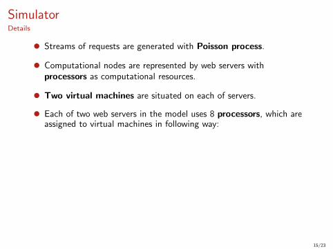
SimulatorDetails

Streams of requests are generated with Poisson process.

Computational nodes are represented by web servers withprocessors as computational resources.

Two virtual machines are situated on each of servers.

Each of two web servers in the model uses 8 processors, which areassigned to virtual machines in following way:

6 and 2 processors are respectively used by first and second virtualmachine (first server).

4 and 4 processors are respectively used by first and second virtualmachine (second server).

Processing delays for web servers are equal 0.0004 seconds and forvirtual machines are equal 0.0008 secondsAccording to the technical report: Lite Technologies, Web server performance comparison: Litespeed 2.0 vs..

15/23

SimulatorDetails

Streams of requests are generated with Poisson process.

Computational nodes are represented by web servers withprocessors as computational resources.

Two virtual machines are situated on each of servers.

Each of two web servers in the model uses 8 processors, which areassigned to virtual machines in following way:

6 and 2 processors are respectively used by first and second virtualmachine (first server).

4 and 4 processors are respectively used by first and second virtualmachine (second server).

Processing delays for web servers are equal 0.0004 seconds and forvirtual machines are equal 0.0008 secondsAccording to the technical report: Lite Technologies, Web server performance comparison: Litespeed 2.0 vs..

15/23

SimulatorDetails

Streams of requests are generated with Poisson process.

Computational nodes are represented by web servers withprocessors as computational resources.

Two virtual machines are situated on each of servers.

Each of two web servers in the model uses 8 processors, which areassigned to virtual machines in following way:

6 and 2 processors are respectively used by first and second virtualmachine (first server).

4 and 4 processors are respectively used by first and second virtualmachine (second server).

Processing delays for web servers are equal 0.0004 seconds and forvirtual machines are equal 0.0008 secondsAccording to the technical report: Lite Technologies, Web server performance comparison: Litespeed 2.0 vs..

15/23

SimulatorDetails

Streams of requests are generated with Poisson process.

Computational nodes are represented by web servers withprocessors as computational resources.

Two virtual machines are situated on each of servers.

Each of two web servers in the model uses 8 processors, which areassigned to virtual machines in following way:

6 and 2 processors are respectively used by first and second virtualmachine (first server).

4 and 4 processors are respectively used by first and second virtualmachine (second server).

Processing delays for web servers are equal 0.0004 seconds and forvirtual machines are equal 0.0008 secondsAccording to the technical report: Lite Technologies, Web server performance comparison: Litespeed 2.0 vs..

15/23

SimulatorDetails

Streams of requests are generated with Poisson process.

Computational nodes are represented by web servers withprocessors as computational resources.

Two virtual machines are situated on each of servers.

Each of two web servers in the model uses 8 processors, which areassigned to virtual machines in following way:

6 and 2 processors are respectively used by first and second virtualmachine (first server).

4 and 4 processors are respectively used by first and second virtualmachine (second server).

Processing delays for web servers are equal 0.0004 seconds and forvirtual machines are equal 0.0008 secondsAccording to the technical report: Lite Technologies, Web server performance comparison: Litespeed 2.0 vs..

15/23

SimulatorDetails

Streams of requests are generated with Poisson process.

Computational nodes are represented by web servers withprocessors as computational resources.

Two virtual machines are situated on each of servers.

Each of two web servers in the model uses 8 processors, which areassigned to virtual machines in following way:

6 and 2 processors are respectively used by first and second virtualmachine (first server).

4 and 4 processors are respectively used by first and second virtualmachine (second server).

Processing delays for web servers are equal 0.0004 seconds and forvirtual machines are equal 0.0008 secondsAccording to the technical report: Lite Technologies, Web server performance comparison: Litespeed 2.0 vs..

15/23

SimulatorDetails

Streams of requests are generated with Poisson process.

Computational nodes are represented by web servers withprocessors as computational resources.

Two virtual machines are situated on each of servers.

Each of two web servers in the model uses 8 processors, which areassigned to virtual machines in following way:

6 and 2 processors are respectively used by first and second virtualmachine (first server).

4 and 4 processors are respectively used by first and second virtualmachine (second server).

Processing delays for web servers are equal 0.0004 seconds and forvirtual machines are equal 0.0008 secondsAccording to the technical report: Lite Technologies, Web server performance comparison: Litespeed 2.0 vs..

15/23

SimulatorModelling Web services

Performance of real data processing services implemented in PlaTelwas modelled: Naive Bayes, Logistic Regression, J48 andMultilayer Perceptron.

Processing time for each of selected services was modelled withtriangular distribution.

The values parameters for distributions (minimum, maximum andaverage value) for each of services were estimated using soapUItool.

Following resource allocation of web services were proposed:

Multilayer Perceptron - total number of 10 processors. Logistic Regression total number of 10 processors. J48 total number of 6 processors. Naive Bayes total number of 4 processors.

16/23

SimulatorModelling Web services

Performance of real data processing services implemented in PlaTelwas modelled: Naive Bayes, Logistic Regression, J48 andMultilayer Perceptron.

Processing time for each of selected services was modelled withtriangular distribution.

The values parameters for distributions (minimum, maximum andaverage value) for each of services were estimated using soapUItool.

Following resource allocation of web services were proposed:

Multilayer Perceptron - total number of 10 processors. Logistic Regression total number of 10 processors. J48 total number of 6 processors. Naive Bayes total number of 4 processors.

16/23

SimulatorModelling Web services

Performance of real data processing services implemented in PlaTelwas modelled: Naive Bayes, Logistic Regression, J48 andMultilayer Perceptron.

Processing time for each of selected services was modelled withtriangular distribution.

The values parameters for distributions (minimum, maximum andaverage value) for each of services were estimated using soapUItool.

Following resource allocation of web services were proposed:

Multilayer Perceptron - total number of 10 processors. Logistic Regression total number of 10 processors. J48 total number of 6 processors. Naive Bayes total number of 4 processors.

16/23

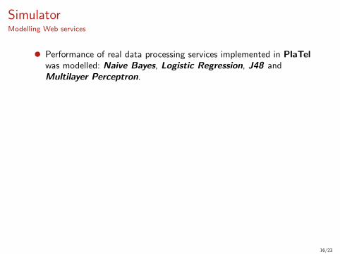
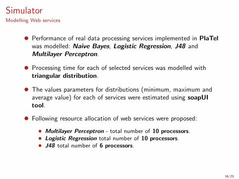
SimulatorModelling Web services

Performance of real data processing services implemented in PlaTelwas modelled: Naive Bayes, Logistic Regression, J48 andMultilayer Perceptron.

Processing time for each of selected services was modelled withtriangular distribution.

The values parameters for distributions (minimum, maximum andaverage value) for each of services were estimated using soapUItool.

Following resource allocation of web services were proposed:

Multilayer Perceptron - total number of 10 processors. Logistic Regression total number of 10 processors. J48 total number of 6 processors. Naive Bayes total number of 4 processors.

16/23

SimulatorModelling Web services

Performance of real data processing services implemented in PlaTelwas modelled: Naive Bayes, Logistic Regression, J48 andMultilayer Perceptron.

Processing time for each of selected services was modelled withtriangular distribution.

The values parameters for distributions (minimum, maximum andaverage value) for each of services were estimated using soapUItool.

Following resource allocation of web services were proposed:

Multilayer Perceptron - total number of 10 processors.

Logistic Regression total number of 10 processors. J48 total number of 6 processors. Naive Bayes total number of 4 processors.

16/23

SimulatorModelling Web services

Performance of real data processing services implemented in PlaTelwas modelled: Naive Bayes, Logistic Regression, J48 andMultilayer Perceptron.

Processing time for each of selected services was modelled withtriangular distribution.

The values parameters for distributions (minimum, maximum andaverage value) for each of services were estimated using soapUItool.

Following resource allocation of web services were proposed:

Multilayer Perceptron - total number of 10 processors. Logistic Regression total number of 10 processors.

J48 total number of 6 processors. Naive Bayes total number of 4 processors.

16/23

SimulatorModelling Web services

Performance of real data processing services implemented in PlaTelwas modelled: Naive Bayes, Logistic Regression, J48 andMultilayer Perceptron.

Processing time for each of selected services was modelled withtriangular distribution.

The values parameters for distributions (minimum, maximum andaverage value) for each of services were estimated using soapUItool.

Following resource allocation of web services were proposed:

Multilayer Perceptron - total number of 10 processors. Logistic Regression total number of 10 processors. J48 total number of 6 processors.

Naive Bayes total number of 4 processors.

16/23

SimulatorModelling Web services

Performance of real data processing services implemented in PlaTelwas modelled: Naive Bayes, Logistic Regression, J48 andMultilayer Perceptron.

Processing time for each of selected services was modelled withtriangular distribution.

The values parameters for distributions (minimum, maximum andaverage value) for each of services were estimated using soapUItool.

Following resource allocation of web services were proposed:

Multilayer Perceptron - total number of 10 processors. Logistic Regression total number of 10 processors. J48 total number of 6 processors. Naive Bayes total number of 4 processors.

16/23

ExperimentDescription

The aim of the experiment is to compare the performance offrequentist approaches with Bayesian approach for change detectionproblem.

Following dissimilarity measures were considered:

Bhattacharyya Kullback-Leibler Lin-Wong modified Lin-Wong

Average latency in request responses was considered as a qualityrate for entire system.

The simulation model was implemented in discrete events simulationenvironment Arena.

Algorithms for change detection were implemented in Matlab.

17/23

ExperimentDescription

The aim of the experiment is to compare the performance offrequentist approaches with Bayesian approach for change detectionproblem.

Following dissimilarity measures were considered:

Bhattacharyya Kullback-Leibler Lin-Wong modified Lin-Wong

Average latency in request responses was considered as a qualityrate for entire system.

The simulation model was implemented in discrete events simulationenvironment Arena.

Algorithms for change detection were implemented in Matlab.

17/23

ExperimentDescription

The aim of the experiment is to compare the performance offrequentist approaches with Bayesian approach for change detectionproblem.

Following dissimilarity measures were considered:

Bhattacharyya

Kullback-Leibler Lin-Wong modified Lin-Wong

Average latency in request responses was considered as a qualityrate for entire system.

The simulation model was implemented in discrete events simulationenvironment Arena.

Algorithms for change detection were implemented in Matlab.

17/23

ExperimentDescription

The aim of the experiment is to compare the performance offrequentist approaches with Bayesian approach for change detectionproblem.

Following dissimilarity measures were considered:

Bhattacharyya Kullback-Leibler

Lin-Wong modified Lin-Wong

Average latency in request responses was considered as a qualityrate for entire system.

The simulation model was implemented in discrete events simulationenvironment Arena.

Algorithms for change detection were implemented in Matlab.

17/23

ExperimentDescription

The aim of the experiment is to compare the performance offrequentist approaches with Bayesian approach for change detectionproblem.

Following dissimilarity measures were considered:

Bhattacharyya Kullback-Leibler Lin-Wong

modified Lin-Wong

Average latency in request responses was considered as a qualityrate for entire system.

The simulation model was implemented in discrete events simulationenvironment Arena.

Algorithms for change detection were implemented in Matlab.

17/23

ExperimentDescription

The aim of the experiment is to compare the performance offrequentist approaches with Bayesian approach for change detectionproblem.

Following dissimilarity measures were considered:

Bhattacharyya Kullback-Leibler Lin-Wong modified Lin-Wong

Average latency in request responses was considered as a qualityrate for entire system.

The simulation model was implemented in discrete events simulationenvironment Arena.

Algorithms for change detection were implemented in Matlab.

17/23

ExperimentDescription

The aim of the experiment is to compare the performance offrequentist approaches with Bayesian approach for change detectionproblem.

Following dissimilarity measures were considered:

Bhattacharyya Kullback-Leibler Lin-Wong modified Lin-Wong

Average latency in request responses was considered as a qualityrate for entire system.

The simulation model was implemented in discrete events simulationenvironment Arena.

Algorithms for change detection were implemented in Matlab.

17/23

ExperimentDescription

The aim of the experiment is to compare the performance offrequentist approaches with Bayesian approach for change detectionproblem.

Following dissimilarity measures were considered:

Bhattacharyya Kullback-Leibler Lin-Wong modified Lin-Wong

Average latency in request responses was considered as a qualityrate for entire system.

The simulation model was implemented in discrete events simulationenvironment Arena.

Algorithms for change detection were implemented in Matlab.

17/23

ExperimentDescription

The aim of the experiment is to compare the performance offrequentist approaches with Bayesian approach for change detectionproblem.

Following dissimilarity measures were considered:

Bhattacharyya Kullback-Leibler Lin-Wong modified Lin-Wong

Average latency in request responses was considered as a qualityrate for entire system.

The simulation model was implemented in discrete events simulationenvironment Arena.

Algorithms for change detection were implemented in Matlab.

17/23

ExperimentConsidered scenarios (1)

1. Slight context change. Thecontext is changed periodically (5times per simulation) and change isgained by increasing the intensityparameters of Poisson process threetimes.

2. Significant context change. Thecontext is changed periodically (5times per simulation) and change isgained by increasing the intensityparameters of Poisson process sixtimes.

18/23

ExperimentConsidered scenarios (2)

3. Processors failure (anomaly).Anomaly is gained by failure of 4processors on first virtual machine.

19/23

ExperimentResults for slight context change simulation

Correctly Incorrectlydetected detected

Measure (max. 5)

Bhattacharyya(L = 25, σ = 0.2) 3.2 0.2Kullback-Leibler(L = 25, σ = 1) 3.8 0.8Lin-Wong(L = 25, σ = 0.15) 2.8 0.7mod. Lin-Wong(L = 25, σ = 0.02) 2.9 0.9

Bayesian approach(L = 25) 3 0.2

20/23

ExperimentResults for significant context change simulation

Correctly Incorrectlydetected detected

Measure (max. 5)

Bhattacharyya(L = 25, σ = 0.2) 4.6 0.1Kullback-Leibler(L = 25, σ = 1) 4.8 0.2Lin-Wong(L = 25, σ = 0.15) 4.6 0.3mod. Lin-Wong(L = 25, σ = 0.02) 4.6 0.2

Bayesian approach(L = 25) 5 0

21/23

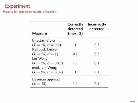
ExperimentResults for processors failure simulation

Correctly Incorrectlydetected detected

Measure (max. 2)

Bhattacharyya(L = 25, σ = 0.2) 1 0.3Kullback-Leibler(L = 25, σ = 1) 0.7 0.3Lin-Wong(L = 25, σ = 0.15) 1.1 0.1mod. Lin-Wong(L = 25, σ = 0.02) 1 0.1

Bayesian approach(L = 25) 1.1 0.1

22/23

Discussion

Most of changes were successfully detected using frequentist andBayesian approaches.

The lowest number of detected changes were gained for Slightcontext change and Processors failure simulation scenarios.

Bayesian approach performed slightly better for Significant contextchange and Processors failure (anomaly) scenarios.

The number of incorrectly detected changes using Bayesian modelwas the lowest for all considered scenarios.

The best results for slight context changes were gained usingBhattacharyya measure.

Bayesian approach, in comparison to the frequentist approach, doesnot demand defining additional parameters beside shifting window’ssize.

23/23

Discussion

Most of changes were successfully detected using frequentist andBayesian approaches.

The lowest number of detected changes were gained for Slightcontext change and Processors failure simulation scenarios.

Bayesian approach performed slightly better for Significant contextchange and Processors failure (anomaly) scenarios.

The number of incorrectly detected changes using Bayesian modelwas the lowest for all considered scenarios.

The best results for slight context changes were gained usingBhattacharyya measure.

Bayesian approach, in comparison to the frequentist approach, doesnot demand defining additional parameters beside shifting window’ssize.

23/23

Discussion

Most of changes were successfully detected using frequentist andBayesian approaches.

The lowest number of detected changes were gained for Slightcontext change and Processors failure simulation scenarios.

Bayesian approach performed slightly better for Significant contextchange and Processors failure (anomaly) scenarios.

The number of incorrectly detected changes using Bayesian modelwas the lowest for all considered scenarios.

The best results for slight context changes were gained usingBhattacharyya measure.

Bayesian approach, in comparison to the frequentist approach, doesnot demand defining additional parameters beside shifting window’ssize.

23/23

Discussion

Most of changes were successfully detected using frequentist andBayesian approaches.

The lowest number of detected changes were gained for Slightcontext change and Processors failure simulation scenarios.

Bayesian approach performed slightly better for Significant contextchange and Processors failure (anomaly) scenarios.

The number of incorrectly detected changes using Bayesian modelwas the lowest for all considered scenarios.

The best results for slight context changes were gained usingBhattacharyya measure.

Bayesian approach, in comparison to the frequentist approach, doesnot demand defining additional parameters beside shifting window’ssize.

23/23

Discussion

Most of changes were successfully detected using frequentist andBayesian approaches.

The lowest number of detected changes were gained for Slightcontext change and Processors failure simulation scenarios.

Bayesian approach performed slightly better for Significant contextchange and Processors failure (anomaly) scenarios.

The number of incorrectly detected changes using Bayesian modelwas the lowest for all considered scenarios.

The best results for slight context changes were gained usingBhattacharyya measure.

Bayesian approach, in comparison to the frequentist approach, doesnot demand defining additional parameters beside shifting window’ssize.

23/23

Discussion

Most of changes were successfully detected using frequentist andBayesian approaches.

The lowest number of detected changes were gained for Slightcontext change and Processors failure simulation scenarios.

Bayesian approach performed slightly better for Significant contextchange and Processors failure (anomaly) scenarios.

The number of incorrectly detected changes using Bayesian modelwas the lowest for all considered scenarios.

The best results for slight context changes were gained usingBhattacharyya measure.

Bayesian approach, in comparison to the frequentist approach, doesnot demand defining additional parameters beside shifting window’ssize.

23/23