i

JOURNAL OF COMPUTATIONAL AND APPLIED MATHEMATICS

ELSEVIER Journal of Computational and Applied Mathematics 67 (1996) 147-159

On Hermite interpolation by Cauchy-Vandermonde systems: the Lagrange formula, the adjoint and the inverse of a

Cauchy-Vandermonde matrix

G. Mi. ih lbach

Institut fffr Angewandte Mathematik, Universit~t Hannover, Welfengarten 1, D-30167 Hannover, Germany

Received 30 August 1994

Abstract

For a given Cauchy-Vandermonde system and for given multiple nodes a Lagrange-type formula for the interpolant is derived, interpolating a given function in the sense of Hermite. We give explicit analytic representations of the basic functions in terms of the nodes and prescribed poles. They are used to derive formulas for the entries of the adjoint of the confluent Cauchy-Vandermonde matrix corresponding to the interpolation problem thus providing an explicit repres- entation of its inverse.

Keywords: Cauchy-Vandermonde systems; Hermite interpolation; Inverse of a Cauchy-Vandermonde matrix

AMS classification: 42A05; 42A20; 65D05

1. Cauchy-Vandermonde systems

Suppose we are given a sequence ~ = (b l ,b2 , . . . ) of not necessarily distinct points of the extended complex plane (~ = Cw { oe }. With ~ we associate a system o/ /= (Ul, u2, . . . ) of basic rational functions defined by

z~(b') if bj = ~ , uj(z) [ (z - bj)-~J(bJ)- t if bj • C. (I)

Here vj(b) denotes the multiplicity of b in the sequence (b l , . . . , b~_ 1). The system q/wi l l be called the Cauchy-Vandermonde system associated with the pole sequence ~ . For any k • N fixed with the initial section of

~k := (bl, . . . , bk) (2)

there corresponds the basis

q/k := (UI, . . . , u~) (3)

0377-0427/96/$15.00 © 1996 Elsevier Science B.V. All rights reserved SSDI 0 3 7 7 - 0 4 2 7 ( 9 4 ) 0 0 1 1 6 - 2

148 G. Miihlbach / Journal o f Computational and Applied Mathematics 67 (1996) 147-159

of the k-dimensional Cauchy-Vandermonde space span q/k. It is well known 1-3, 4] that for every k, q/k is an extended complete Ceby§ev system on C \ {bl .... , bk }, in particular for k e N fixed and for any given system

~'k := (a l , . . . , ak) (4)

of not necessarily distinct complex numbers a~ and for any complex functionfwhich is defined and sufficiently smooth at the nodes a~ there is a unique element u e span ~k satisfying the interpolation conditions

z] (u -- f ) (al) = 0 (i = 1, . . . ,k) . (5)

Here I-ti(a) denotes the multiplicity of a in the sequence (al, ..., al-1). In I-2, 3] a Neville-Aitken formula and in [5] a Newton formula computing the interpolant u recursively are given. The aim of this note is twofold. First we are going to derive a Lagrange-type formula

k (d)U,( , , ) u(z) = i:,E li(z)\~zz ] f(al). (6)

More precisely, we will derive explicit representations of the basic Lagrange functions l~ in terms of the nodes (4) and the poles (2) involved. Of course, if all poles are prescribed to be at infinity this result must contain the well-known Lagrange-Hermite formula for interpolation by algebraic polynomials which can be found in [1]. In a second step we will use the representations of the basic rational functions l~ to compute the entries of the inverse of the Cauchy-Vandermonde matrix

V:--- t / ? ~ a . \ ' l j = 1 . . . . . k ~ N ~ i ' ' J / . t i= l ..... k ' (7)

where by Li we denote the Hermite functionals

d "y"(') f ~ (L , , f ) = \-~zJ f (ai ) . (8)

2. The Lagrange formula

The basic Lagrange functions lj ( j = 1 , . . . , k) for the k-dimensional Cauchy-Vandermonde space span q/k are uniquely determined by the conditions of biorthogonality

(Li , l j ) = fii.j (i,j = 1, . . . ,k) .

G. Miihlbach / Journal of Computational and Applied Mathematics 67 (1996) 147-159 149

Evidently,

1

lj - det V

( L I , u l ) "'" ( L l , U k )

( L j - 1, Ill ) "'" (L~_ 1, Uk)

II 1 . . . l,l k

( L j + I , u l ) "'" ( L j + l , U k )

( Lk , U l ) "'" ( Lk , Uk )

(9)

where V is the confluent C a u c h y - V a n d e r m o n d e matrix (7) and where the numera to r de terminant is defined by its formal Laplacian expansion along its j t h row. Obviously, knowing the coefficients cj, t of the expansion

k

I j = ~ % t ' u , ( j = l , . . . , k ) , (10) t = l

this yields explicit representat ions of the adjoint and of the inverse of V. In fact, the adjoint Vaaj of \ t = 1 . . . . . k V equals det V. C T, where C := tcj, tJj= 1 ..... k, hence

V - 1 = C T. (1 1)

There is an explicit formula for det V provided the nodes and poles are consistently ordered, i.e.

d k = (al , . . . , ak ) = ( ~ 1 , . . - , ~ 1 , g 2 , . . . , % - 1 , % , . . . , % ) , (12) k Y ) k

m 1 mp

~ k = ( b l , . . . , b k ) = (f i t , ... , i l l , f12, . . . , f l q - 1 , f lq , . . . , f lq) , (13)

n I nq

where ~1, .-. ,%, fi t , - . . ,flq are pairwise distinct and ml + ..- + m p -- k and nl + ,.- + nq = k. Under these assumpt ions the C a u c h y - V a n d e r m o n d e matrix (7) has the determinant

[-Ii,j=l"k (a i -- aj) I-]:kj=1 (bi - bj)

det V = m u l t ( d t ) " i>~ i>j (14) * (ai b~) ,k

1-]i , j= l 1 - - r l i j = (b i - aj) i> . j i > j

which was derived in [3] (cf. also [2, 4]). Here we use the notat ions

k

mult (agk) = 1-I Pi(a~)! i = 1

and for a finite index set J and elements ?j e (~

1-I* FI j ~ J j ~ J

1 5 0 G. Miihlbach / Journal of Computational and Applied Mathematics 67 (1996) 147-159

with

1 i f f T j = 0o or ? j = 0 ,

i := iff E C \ {0} .

Of course, there is no loss of generality in assuming that the nodes and poles are ordered consistently. This only means reordering the system ~k keeping it to be an extended complete t~eby~ev system on C \ { b l , ... ,bk} and reordering the sum (6) according to the permutat ion of ~'k to get the node system consistently ordered. Assuming consistently ordered systems (12) and (13) leads to a simple sign factor in the determinant (14).

In order to derive an explicit representation of the inverse of V it is important that we can change easily between the one-index enumerations of the Hermite functionals (8) corresponding to the one-index enumerat ion of the nodes (4) and the two-index enumerat ion

( L i , f } = f ( ~ r ) ( r = l , . . . , p ; p = O . . . . , m r - l ) . (15)

This is done by the one-to-one correspondence

~O .

(r,p) w-~t=cp(r ,p):=ma + "" + m , - 1 + P + I (16)

shown in the table

(r,p) (1,0) (1,1) ... (1,m 1 - 1 ) (2,0) ... (2,m 2 - 1 ) ... (r,p) ... (p, m p - 1 )

i = ~p(r,p) 1 2 . . . m I m 1 + 1 ... ml + m 2 " ' " ml + " " + mr-1 + P + 1 ... k

Similarly, the two enumerations of the Cauchy-Vandermonde functions (3) corresponding to the one-index enumerat ion (2) of the poles and the two-index enumerat ion

Uj = U,n, u (m = l . . . . . q; lt = l , . . . , n m ) ,

where

:= ( Z - - t i m ) u' m = l . . . . . q - - l ; p = l . . . . ,n,,,

(17) z u - l , m = q ; p = l . . . . ,nq

is realized by the one-to-one mapping

(m, It) ~-~j = ~k(m, #) = n l + ..- + n,,_l + It. (18)

Observe that for convenience we assume the pole m to be represented by flq.

G. Miihlbach / Journal o f Computational and Applied Mathematics 67 (1996) 147-159 151

In order to derive a Lagrange- type formula (6) we need some nota t ion:

k q - 1

Q(z) := H * ( z - b~) = H (z - fit)"', j = l t = l

P

COl(Z):= 1-I (z - (l = l , . . . , p ) , s = l , s ¢ . l

vl, a ( z ) : = ~ . ( z - ~ t ) z ( l = l . . . . , p ; 2 = O , . . . , m z - 1 ) ,

i

i = O

= Taylor ' s po lynomia l of order mt - )~ - 1 of the funct ion Q/COt developed at the point z = 0~t,

d / ( ' ) : = (-)~=~, ( l = l . . . . , p ; i = O , . . . , m l - 1 ) . (19)

Theorem 1. Assume that the node system (3) and the pole system (2) are disjoint. Suppose that these systems when consistently ordered are identical with (12) and (13), respectively. Then the Lagrange- type basis functions (9) are

l~o(t,a)(z):= COtZ(z): = COt(z) Pt x(z)" vz, a(z) (l = 1 . . . . ,p; 2 = 0 , . . ,ml - 1). (20) Q(z) "

The functions CO{ ~ span q/k are uniquely determined by the biorthogonality relations

d~CO~s t =6<s,~),~,a)=6~,~'6~.~ ( s = I, . . . . . . , p ; a = 0 , . , m s - 1 ) , ( l = l , . . , p ; 2 = 0 , . . . , m ~ - I).

(21)

Proof. By part ial f ract ion decompos i t ion first we observe that CO/e span ~k for all l = 1, . . . , p and 2 = 0, . . . , mt - 1. Moreover , if s ¢ I then in view of Leibniz' rule d7 CO¢ = 0 since then CO/contains the factor (z - es) "~. Supposing now s = I we mus t show that

dTCOX=fi~,~ (a, 2 = 0 , . . . , m z - 1 ) .

Again, by Leibniz' rule this is clear for o- < 2. W h e n a >~ 2 this is equivalent with

dT(u'v) = 6~,a (2 <~ ff ~ ml -- 1),

where we have set u := COt'Pz,a/Q and v := vl, a and dl is defined by (19). Using Leibniz' rule repeatedly we find

• = a , = . d f ( ~ t ' ] d ~ ~ op~,~. p=O P

152 G. Miihlbach / Journal o f Computational and Applied Mathematics 67 (1996) 147-159

But it is easily seen that dT-a-PPt , a = dT-a-P(Q/~ot) for 0 ~< o - 2 - p ~< mt - 2 - 1. Therefore,

In view of a well-known theorem of linear algebra as an immediate consequence of the bior- thogonal i ty relations (21) we have the following corollary.

Corollary. Under the assumptions o f Theorem 1 there holds the La#ranoe-Hermite interpolation formula

u(z) = Z Z wtx(z) f(oc,), / = 1 2 = 0

which is identical with (6) after renumberin# the basic Laoranae functions and the Hermite functionals accordin9 to q~ [c f (16)].

3. Partial fraction decomposition of the Lagrange basis functions

The aim of this section is to compute the coefficients t" ~ Am,u of the partial fraction decomposi t ion

q nm

o)? Z Z ,,a (22) = Am, u" urn, u , m = l /~=1

where ~@ is given in Theorem 1 and urn, t* is defined by (17). We will give explicit formulas for the 1,2 Am., in terms of the nodes and poles involved. Mult iplying (22) by Q (z) we see that this equat ion is equivalent with

oh(z) Pt, a(z) v,,a(z) ,,a • " = A m , t, H (Z - - f i t ) n' (Z - - t im) n--I~ t * = l t = l , t # m

+ Q(z) • A~:Zu'z t*-a. (23) t * = l

We shall make use of the shor thand notat ions

D,~(-):= (')z=a. (m = 1 . . . . ,q ;z = 1 . . . . ,nm).

Theorem 2. Under the assumptions o f Theorem 1 we have for every l = 1 . . . . , p; 2 = 0 . . . . , mt - 1

1,2 A m , t* -~-

D n. -u [o~t" Pt, a" vl. a]

(rim - - Z ) ! m (Bin - - B,)"'

(nq -- P)! [_ Q (z)" z"'- 1 J

/ f m = 1 , . . . , q - 1;/~ = 1, . . . ,nm,

i f m = q ; ~ = 1 . . . . ,n~.

(24a)

(24b)

G. Miihlbach / Journal o f Computational and Applied Mathematics 67 (1996) 147-159 153

Proof. Formula (24a) results immediately by applying D~,'-U/(n m - - 1 1 ) ! to both sides of (23) in view of Leibniz' rule. Similarly, (24b) results by applying D~,-~'/(nq - p)! to both sides of the equation obtained by dividing (22) by z "~- ~. []

In order to express the coefficients *' ~ Am.u in terms of the nodes and poles explicitly we have to carry out some elementary but tedious calculations. To begin with we compute first the coefficients of the polynomial P~, a. Once more we use Leibniz' formula

\ ~ , / j~=o d/Q'd~-J

and express d[Q and dh(1/o~t) separately. Let us introduce the shorthand notations

Zl:= z - o~z, Y, , l := fit - - O~l, Z s , l : : O~s - - O~l.

Then q - 1 q - 1 q - 1 n, nt _ _

Q(z) = I-I ( z - fl,)", = [I ( z , - Yt,,)", = I-I ~ z [ , ( - Yt.,)",-', = ~ ~.' .d/Q, t = l t = l t = l ~,=0 Tt j !

with

d/Q =j~ E (~1, ...,%-Octavo -t ~l+.-. +~q_t=j

On the other side,

(n , ) . . .(nq_,"}(_ y , l ) n _ . r . . . . (__ yq_l,,),,,,_ _~.,_ ' 1~1 •q- 1 // '

(25)

1 P 1

- 1-[ , ( z - ~ X " ~,(z) s=,,,,

where

1 (-- 1 )m ' - l (d ) m'-I 1

and in a neighborhood of at

1 _ 1 1 1 £ (Z , ' ] " z - ~, Z,,, 1 - - ( Z t / Z , , , ) = Z , ,~ ,,=o \Z-~,lfl "

Therefore, by termwise differentiation we get

1 1 ~ ( V s + m s - 1 ) ( Z t ~ v" (z - o~ )" . - z,."~ ,, .=o v, \~l

and

1 ~o,(z)

. , l ' s = l s = l vs=O s ~ l s # l

1 5 4 G. Miihlbach / Journal of Computational and Applied Mathematics 67 (1996) 147-159

where

( f i 1 / ( v l + m l - - 1 ) . . . ( V p + m p - - 1 ) 1 dh[± = Y , v , v . . . .

l ~WlJ s=l z '~/ ,S,(v . . . . . . v , )~ l%lo , \ Z l , l s # l / vt+'" +vp=h, vt=0

(26)

Putting things together we finally get

~.d; = FI s = l , s O l

i ( (nl) (nq_l~ (__ 1,1) nq-l-~q- x E E , "'" YI . ' ) "'-~ . . . . ( - Yq- j=o|tt ...... ~,-,)~o-' zl \ z q - l J

~tl +'" +zq_j=j

× ~ ( v l + m l - 1 )

(v~, . . . , v D e No p , V l vt+... +vp=i- j , ¥1mO v~ Z?., . Z~,"

(27)

Next we calculate the numerator of the expression (24a). We have to expand the polynomial ol(x)" Pl, a(x)'vz.~(x) at x = tim. Using the shorthand notations

X m ' ~ - X - - flm and Ym,~:= flm -- ~s,

we get

P ) 1 m , - 2 - 1 d[(Q/@) (x - at) i+ a w,(x) 'Pt , z(x) 'v, ,a(x) = I-] (x - as) =" -~. i~=o i!

s = l , s # l

( s = l , s ~ l

y , . ) 1 m,-z- ld[(Q/( .Ol) (Xm+ v ii+Z (Xm + m.,) ' ~.. Z i! ",n.,, •

i=O

By making use of the binomial theorem and by interchanging the order of summation the last sum can be written

rot--1 ( mt--~--i ( ) ( ) ) XPm, 1 Q p + 2 r~,+ta_.,

p,=O \p=max(O,p,-z) P -'~" d~ -~l Pl

Therefore

rim-- 1 (2), (x) " Pz, a (x)" v,. a (x)

j = O

x~ 7 D~ [~o,- P,. ~. v,, ~] + ¢(x~-),

G. Miihlbach / Journal of Computational and Applied Mathematics 67 (1996) 147-159 155

with

(p ...... p,)eN~ D1 \ P l - 1 / i m, l ra, l - 1 pl + ... +pl=j

X p = m a x ( O , Pz- ~) Pl

(?n/+l'~ (rap) ~m,+,-p,+t ymp-p~, X "'" " ''"

\ P l + l ,I pp - - re , l + 1 m , p "

It remains to compute the derivatives occurring in (24b) in terms of the nodes and poles. We will do this by expanding tnl(z)" Pl, a(z)" vl, x(z) /(Q(z)'z ":1 ) into a Laurent series around zero:

o,(z).P,.x(z).v,.x(Z)Q(z) "z"-I = •", A~,a.z.l_, . + (9(1) / x = l

= Z ; , , , _ , - ~ + e , z - ~ . j = 0

We use the Laurent series of a typical factor of Q which is

1 _ 1 ~ ( v + n - 1 ) ( ~ ) ' (z -/~)" z",=0 v

and Taylor's expansion around zero of the numerator which reads

~,(z) 'P, ,~(z)'v~,~(z)=~ [ l ( z - ~ ) ~" df (Q/°~' ) ( z -~ , ) p+~ s=l,s~z p=o P!

(28)

1(:, (:':; = ~ z"( - ~,)~.,-o,

s = l p~=O s ~ l

\p,=o ,,,=max{O,p,- ~} Pl P! ]

~ pl + "" + p ~ = j

X

mr- ; t - 1

O = m a x { O , o : ;t }

+ d:(Q/~o,)']

\Pl+1} \Pp,/

156 (2[ Miihlbach / Journal of Computational and Applied Mathematics 67 (1996) 147-159

By expanding each factor of Q according to (28) and by mult iplying these expansions and the Taylor ' s expans ion jus t derived we finally get

60t(z)'Pl, a(Z)'Vl, a(Z) "~l l Az,, t ( 9 ( 1 ) = p ~, ._ j+ ~ , z ~ o o , Q(z) "z"'-I j=o

with

= _ , (v, + n, - , ) ... ... A q ' n " - J 2 ! (v ...... v,)el~[ Vl V q - 1

v~ + ... +vq=j

ta ...... a,)~g Pl \ P l - 1 } [ p l + . . . + p p = k - l - v q

X

m ~ - A - 1

Z p = m a x { O , m - 2}

p + 2 ) ( _ ~)~+ ,_~, df(9./co3 Pl P! )

x/|m'+' \ / "X}.../mp}(_ 0C1+1) m'+ ' -p . . . . . . ( - - O ~ p ) mp-pp ( j = O, ...,%-1). \Pt+ l } \Pp /

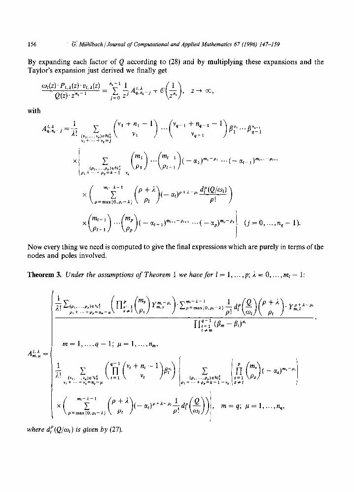
N o w every thing we need is c o m p u t e d to give the final expressions which are pure ly in terms of the nodes and poles involved.

Theorem 3. Under the assumptions of Theorem 1 we have for l = 1 , . . . , p; 2 = 0 . . . . , mt - l:

l,). Am, kt

, ( ( ) ~..~(p ...... o,)'"g ~-[f=, ms y m - p ~ V=' -*-1 P+~" vp+a -p , p , + ... + p , = n = - # \ s # l p , m:'s ' ) '=a=m,x{O, , , -a} . d a Pl " -= , l

q - 1 Ht=l ( t im - - f i t ) n' t ~ m

m = 1 , . . . , q - 1; /~ = 1 , . . . , n , , ,

(Vl,-.., Vq)~ N~ Vt (Pl, ..., pp) e N g v l + " " + % = n q - # Pl + "" + p p = k - l - %

x ~ P + 2 (_ ~t)p+~_p, P! p=max{O,p l -2} Pl

where d[ (Q/coz) is given by (27).

s = 1 P s

m = q ; ~ = 1 .... ,nq,

G. Miih lbach / Journal o f Computat ional and App l i ed Mathemat ics 67 (1996) 147-159 157

4. The adjoint and the inverse of a confluent Cauchy-Vandermonde matrix

In view of the general considerations at the beginning of Section 2 from Theorem 3 we obtain

Theorem 4. Under the assumptions of Theorem 1 the adjoint of the Cauchy-Vandermonde matrix (7) equals

V a d j = (det V). C T ,

where det V can be found under (14) and the entries of the matrix C = (cj, i)~%~l'~.[~,

Cj, i ~ : /1 ~p-I(j)

are given in Theorem 3. Here q~-1 and ~p-1 are the inverse functions of (16) and (18), respectively.

Theorem 5. Under the assumptions of Theorem 1 the inverse of the Cauchy-Vandermonde matrix (7) equals

V - 1 = C T = {c. .~i=1 ..... k ', t , J / j = l , . . . , k ,

where the matrix C = (cj, i)~11~~7,~ is defined in Theorem 4.

5. Examples

Example 1. (Simple complex poles and simple nodes: Cauchy's interpolation problem). (a l , . . . , ak ) = (al . . . . ,ak), that means: p = k and ml = 1 for i = 1 , . . . , k ; (bl, . . . ,bk) = (ill . . . . ,ilk), that means q -- 1 = k and ni = 1 for i = 1 , . . . ,k , nq = 0.

Then V is Cauchy's matrix

V =

' ( ~ - t h ) -~ ( ~ - / ~ ) - x ... ( ~ 1 - / ~ ) - "

( ~ - t ~ ) - ~ ( ~ - / h ) - ~ ... ( ~ - t ~ ) - ~

(~ - t h ) - ~ ( ~ - t ~ ) - ~ ... (~ - t ~ ) - ~

By Theorem 4 its adjoint is

/ = 1 .... ,k Vad j = det V (A2, ° m=l ..... k,

where k

I-I (~, - - f i t ) k tim - - O~s l,O t = 1

Ara , 1 ---~ H k s = 1 0~/ - - O~ s

t = l t # m

158

and where f rom (14) we infer

det V = 1-] (el - e~)(fl j - fli) (el - flj). i , j= l i, 1

i> j

By Theo rem 5 the inverse of Cauchy 's matr ix (29) is

C T ( A l , O " t l = l . . . . . k ----- ~,Ara, l im= l , . . . ,k .

The Lagrange basic functions in this case are

G. Miihlbach / Journal o f Computational and Applied Mathematics 67 (1996) 147-159

lj(z) = o9 ° (z) = h z --~__~ h ~j Z fl' s= l , s # j O~j - - O~s t= 1 Z - - f i t

( j = 1 , . . . , k ) .

Example 2. (Taylor 's in terpola t ion at ~ with a C a u c h y - V a n d e r m o n d e system).

(a l . . . . , ak ) = (~1 . . . . , ~ t ) , i.e. p = 1 and np = k;

( b l , . . . , b k ) = ( f l l , . . . , f l l , f l 2 , . . . , f l q - l , f l q , . - - , f l q ) with nl + . . . + nq = k, k ) k )

y y- , f I1 t flq "

fix,-.. ,flq-1 e 12 pairwise distinct and distinct f rom al , f l~/= oo with 0 ~< nq <~ k.

The cor responding C a u c h y - V a n d e r m o n d e matr ix V is

V = (d~us . l j=*(m, ~,)=1 ..... k • 1 2 = 0 . . . . . k - 1

where

dt Um,~ = Tz 1

(z - ~ , . ) " I~--,, =

'( _ 1) a ( p + A - 1)! 1

(~ - 1 ) ! (~Zx - t i m ) ' + ~

if m -- 1 , . . . , q - - 1; /t = 1 , . . . , n m ,

2 ' ( / ~ - 2 1 ) z ' - ' - 2

if m = q; /t = 1 , . . . , n q .

By Theo rem 4 its adjoint is

Vad j det V I ~ ~=o ..... k- I = (Am:,) j=,( . . . , )= l ..... k.

where (cf. [4, p. 81]) *k

det V = o'1 ( j - 1)! i>j j= x I]] k 1 (oq - b j) '

G, Miihlbach / Journal of Computational and Applied Mathematics 67 (1996) 147-159 159

a t = ( - 1) ~' w i th ~ = Z~=l # j (b j ) , a n d w h e r e

1 , 2 A m , / t

I I *-z-'IQ(P+21~) ]/Iqf-I~1 1 Z,., Y' ( & - ( p , . - p = m a x { O , n ~ - p - 2 } glm - - L t ~ m

if m = 1 , . . . , q - 1; # = 1,...,nm,

1 , + t h v, _ _ ( _ 2! ~" )f i t ) [ Z 1 d ( Q P + 2 a l r + ~ - k + l + v . (~ ....... ,),N~ vt / /Lo=~x{O,k_l_~_z} p! -- 1 -- v~

V 1 + ... +V~=tlq--/~

if m = q; # = 1 , . . . , n q ,

w i th

d~Q - n, (~ ..... ~_~)~Nqo -1 T I + "" + T ~ - I = O

By T h e o r e m 5 the inverse o f V is

C T t A Z , ~ a = o ..... k-1 ~- x m , # l j = q / ( m , p ) = 1, . . . ,k "

T h e L a g r a n g e bas ic f u n c t i o n s in this case a re

1 k-~-ld~Q 7 .

w h e r e Q(z) = [-[~k__ 1( z _ b~).

R e f e r e n c e s

[1] J. Berezin and N. Zhidkov, Computing Methods, Vol. 1 (Addison-Wesley, Reading, MA, 1965). [2] C. Carstensen and G. Mfihlbach, The Neville--Aitken formula for rational interpolants with prescribed poles, Numer.

Algorithms 3 (1992) 133-142. [3] M. Gasca, J.J. Martinez and G. Mtihlbach, Computation of rational interpolants with prescribed poles, J. Comput.

Appl. Math. 26 (1989) 297-309. [4] G. Miihlbach, Computation of Cauchy-Vandermonde determinants, J. Number Theory 43 (1993) 74-81. [5] G. Miihlbach, On interpolation by rational functions with prescribed poles and applications to multivariate

interpolation, J. Comput. Appl. Math. 32 (1990) 203-216.