1

On Fluid Compressibility in Switch-Mode Hydraulic Circuits -

Part I: Modeling and Analysis

James D. Van de Ven Department of Mechanical Engineering

Worcester Polytechnic Institute 100 Institute Rd.

Worcester, MA 01609

E-mail: vandeven@wpi.edu Phone: 508-831-6776 Fax: 508-831-5680

June 7, 2011

Revised March 23, 2012

Abstract Fluid compressibility has a major influence on the efficiency of switch-mode hydraulic circuits due to the release of energy stored in fluid compression during each switching cycle and the increased flow rate through the high-speed valve during transition events. Multiple models existing in the literature for fluid bulk modulus, the inverse of the compressibility, are reviewed and compared with regards to their applicability to a switch-mode circuit. In this work, a computational model is constructed of the primary energy losses in a generic switch-mode hydraulic circuit with emphasis on losses created by fluid compressibility. The model is used in a computational experiment where the system pressure, switched volume, and fraction of air entrained in the hydraulic fluid are varied through multiple levels. The computational experiments resulted in switch-mode circuit volumetric efficiencies that ranged from 51% to 95%. The dominant energy loss is due to throttling through the ports of the high-speed valve during valve transition events. The throttling losses increase with the fraction of entrained air and the volume of fluid experiencing pressure fluctuations, with a smaller overall influence seen as a result of the system pressure. The results of the computational experiment indicate that to achieve high efficiency in switch-mode hydraulic circuits, it is critical to minimize both the entrained air in the hydraulic fluid and the fluid volume between the high-speed valve and the pump, motor, or actuator. These computational results are compared to experimental results in part II of this two part paper series. Keywords: switch-mode hydraulic circuit, digital hydraulics, compressibility modeling, bulk modulus 1. Introduction/Background Switch-mode hydraulic circuits provide a compact, efficient, fast response, and low-cost hydraulic control option. While significant research attention has been given to switch-mode hydraulic circuits, the technology has not penetrated the hydraulics industry. The main technical barriers that appear to be preventing the technology from being applied in the industry include the lack of a hydraulic valve capable of high frequency switching with low energy consumption, physical circuits demonstrating lower efficiency than predicted through simulations due to a combination of energy losses, and a general lack of widespread understanding of the circuit behavior. While the author and others are addressing the valve development need through other work, this paper series focuses on developing a deeper understanding of energy losses in a switch-mode circuit with specific focus on the compressibility energy loss, which is unique to this control method. Switch-mode hydraulic circuits, the hydraulic analog of DC-DC switch-mode circuits from power electronics, can be configured in multiple ways. Generally speaking, the circuits consist of a valve that switches the circuit between distinct on and off states, inertial and capacitive energy storage devices to

2

improve the circuit efficiency and smooth pressure pulsations, and possibly a check valve to prevent flow reversal. As seen in Figure 1 a) and b), switch-mode circuits can be used to control a hydraulic source, such as a pump, or a sink, such as a motor or a linear actuator. By utilizing a 3-way high-speed valve and adding a direction reverse valve, four-quadrant control1 of a pump/motor is achieved, as seen in Figure 1 c). Note that the purpose of the check valves in this specific circuit is to prevent pressure spikes during valve transitions when flow through the high-speed valve is blocked. The focus of this paper will be on the control of a hydraulic motor using the 3-way valve circuit, yet the methods employed are applicable to other switch-mode circuit architectures.

Figure 1. Some configurations of switch-mode hydraulic circuits. Circuit a) is a uni-directional virtually variable displacement pump. Circuit b) is a uni-directional virtually variable displacement motor. Circuit c) is a bi-directional virtually variable displacement pump/motor using a 3-way valve and a direction reverse valve that is only used to change the torque direction. The bold fluid paths are defined as the switched volume.

A description of the operation of the switch-mode circuit controlling a hydraulic motor in a bi-directional pump/motor circuit, illustrated in Figure 1 c), is now presented. When the high-speed valve is connecting the P and A ports, flow passes from the high-pressure rail, through the valve and to the motor, applying a torque to the output shaft. When the valve shifts to connect the T and A ports, the rotational inertia of the motor draws flow from tank through the high-speed valve and the check valve. By modulating the duty cycle, defined as the time with the P and A ports connected divided by the switching period, the average torque of the hydraulic motor is controlled. The function of the accumulator is to smooth out pressure variations in the high-pressure rail created by the flow pulsations. As mentioned, a good deal of previous research attention has focused on the design of high-speed hydraulic valves for switch-mode hydraulic circuits. A wide range of valve solutions have been proposed, with literature reviews provided in these references [1; 2]. Within the valve development work and auxiliary to

1 Four-quadrant control is defined as sinking and sourcing power with reversing flow direction, allowing a hydraulic unit to act as a pump and a motor in both rotational directions.

3

it, models have been developed of switch-mode hydraulic circuits. Generally speaking, there are five major sources of energy loss in a switch-mode circuit: internal leakage in the valve, viscous friction in the valve, throttling during fully-open and transitioning events, inertial forces in oscillating valve designs, and fluid compressibility. Work at Purdue University and by Tomlinson et al. modeled the steady and transient throttling losses and the compressibility loss assuming a constant bulk modulus [3-5]. Work at the University of Minnesota has considered all of the above mentioned energy loss terms applicable to a rotary valve, including compressibility with a pressure dependent bulk modulus term [1]. However, the work did not account for the influence of fluid compressibility on the transient throttling loss as further discussed in section 3.3. The focus of this paper is on understanding the role of fluid compressibility on the behavior and efficiency of a switch-mode circuit. Towards this end, a discussion of bulk modulus models is presented in section 2, followed by the development of a computational model of energy losses in a generic switch-mode system in section 3. In section 4, results of a set of computational experiments are presented, followed by a discussion and concluding remarks in sections 5 and 6 respectively. In the appendix, results from the model utilizing different bulk modulus models are presented. In part II of this paper series, the computational results will be compared to the experimental results with a similar switch-mode system [6]. 2. Bulk Modulus of Hydraulic Fluid During each period of operation, the volume of fluid between the valves and the hydraulic sink or source, referred to as the switched volume, is exposed to large pressure fluctuations between the pressure of the accumulator and the tank pressure. Due to compressibility of hydraulic fluid, when the switched volume is connected to high pressure, the mass of fluid in this volume increases. In a pump or pump/motor circuit, as illustrated in Figure 1a) and c), when the switched volume is connected to tank this additional mass of fluid is discharged to the tank. Because fluid mass is added to the switched volume at high pressure and released at low pressure, this results in a loss of energy, defined as the fluid compressibility loss. The inverse of fluid compressibility is the bulk modulus of the fluid, which is defined as the change in pressure required to create a change in volume of a given volume. The average or secant bulk modulus is expressed as [7]:

o

PV

V

(1)

where β is the bulk modulus,Vo is the initial volume, ΔP is the pressure change, and ΔV is the volume change. The dynamic bulk modulus, also known as the tangent bulk modulus, is the differential form of Equation (1), expressed as [7]:

dP

VdV

(2)

where V is the volume at the operating pressure, and dP/dV is the infinitesimal pressure change required to achieve an infinitesimal volume change. The effective bulk modulus of hydraulic fluids is a function of the specific fluid, the entrained air content of the fluid, the operating pressure, and the fluid temperature [8]. Interestingly, the effective bulk modulus is only influenced by the quantity of entrained air and not the air dissolved in the fluid [7]. As described by Henry’s Law, the solubility of air in hydraulic fluid increases with increasing pressure [8]. While the effective bulk modulus of hydraulic fluid can also be influenced by compliance in the fluid conductors, to improve generality, this work will assume perfectly rigid fluid conductors. Numerous effective bulk modulus models of varying complexity have been developed for hydraulic fluids. A simplistic model, as described by Akers et al., can be developed by considering the compressibility of the hydraulic fluid and the entrained air as springs in series [9]:

1 1 1 1 1T a a a

e T T a T a

V V V V

V V V

(3)

where βe is the effective bulk modulus, βa is the bulk modulus of air, Va is the volume of air, and VT is the total volume. The approximate form of Equation (3) uses the assumption that the volume of the fluid

4

divided by the total volume is unity. The air bulk modulus term can be described using isothermal, adiabatic, or polytropic assumptions, based on the rate of pressure change. Multiple isothermal models have been presented in the literature [9; 10]. Due to high frequency pressure pulsations in a switch-mode system, adiabatic behavior is the focus of this paper. Merritt presented the following basic adiabatic model based on the secant bulk modulus [10]:

e

P

R P

(4)

where P is the pressure, γ is the ratio of specific heats for air, and R is the percent air content by volume at atmospheric pressure. Merritt’s model was further developed by Akers to include the decrease in entrained air volume with increased pressure [9]. A more detailed adiabatic model by Hayward, as described by Watton, is based on the tangent bulk modulus and expressed as [11]:

o

e

o

PR

P

R PP P

(5)

where P is the absolute pressure, Po is atmospheric pressure, and γ is the ratio of specific heats for air. Another model was developed by Cho et.al that included the addition of accounting for variable hydraulic fluid density with pressure [12]:

1

1

o

o

P P

oe

P P

o

Pe R

P

R Pe

P P

(6)

Note that that Equation (6) was modified by the author to use absolute pressure instead of gauge pressure as originally presented by Cho et al. Yu et al. developed a theoretical model of the effective bulk modulus that accounts for entrained air dissolving with increasing pressure [13]:

11

1 11

11e

o o

P

P P R c P P P

(7)

where c1 is the coefficient of air bubble volume variation due to the variation of the ratio of the entrained air and dissolved air content in oil with units of (Pa-1); this coefficient is typically found by curve fitting to experimental data. It must be noted that Yu et. al. determined the air bubble variation coefficient, c1, at a low entrained air level of 0.004% volume fraction, where the impact of this coefficient is small. The author has found that at the air levels of interest in this work, the coefficient experimentally selected by Yu et al. results in their model deviating significantly from the other bulk modulus models. Equation (7) was modified by the author from the original form to use absolute pressure instead of gauge pressure. Finally, additional bulk modulus models do exist, including Ruan and Burton’s work utilizing the critical pressure to predict dissolving of the entrained air [14]. A comparison of the effective bulk modulus as a function of pressure using the four bulk modulus models presented in Eqns (4)-(7), provided in Figure 2, reveals significant difference in the predicted values between the various models. For this plot the entrained air content at atmospheric pressure is 2%. The Yu et al. model is plotted twice with the air bubble variation coefficient, c1, set to -9x10-5 Pa-1, as suggested by Yu et al. in an example [13], and -10-7, to demonstrate the impact of this coefficient.

5

0 2 4 6 8 10 12 14 16 18 200

0.2

0.4

0.6

0.8

1

1.2

1.4

1.6

1.8

2

Pressure (MPa)

Bul

k M

odul

us (

GP

a)

Bulk Modulus vs. Pressure for R = 0.02

Yu, c1 = 9e-5

Yu, c1 = 1e-7

ChoHayward

Merritt

Figure 2. Bulk modulus versus pressure with 2% entrained air by volume at atmospheric pressure using the various models found in the literature. Note the Yu et al. model is plotted twice with different values for the air bubble variation coefficient, c1, to demonstrate the impact.

3. Switch-Mode Circuit Energy Loss Model As mentioned previously, there are multiple sources of energy loss in a switch-mode hydraulic circuit. In this section, a model will be developed of the primary energy losses with a focus on understanding the influence of fluid compressibility. While the model developed below addresses the major volumetric energy loss sources, additional energy losses do exist that will not be incorporated into the model. Additional losses include mechanical losses that dependent on the specific valve architecture. Further losses that are excluded from the model include hysteresis in the accumulator, viscous pipe flow losses, and losses in the pump, motor, or actuator. These losses are neglected in order to maintaining focus on the core of the switch-mode circuit. For the purpose of generalizing this work, a bi-directional pump/motor switch-mode circuit, illustrated in Figure 1 c), operating as a motor and utilizing off-the-shelf parts, will be considered. Only considering commercially available components limits the performance of the circuit due to limitations in the valve transition time and thus switching frequency. This trade-off is worthwhile as it enables broad application of this computational work and provides direct comparison to the experimental work that will be presented in the second part of this paper series [6]. The individual sources of energy loss will now be developed, followed by a presentation of the component parameters in section 4. 3.1 Valve Actuation Energy Loss To perform the high frequency switching required for switch-mode control, energy is required to operate the valve to overcome viscous friction between moving components in the valve and inertial forces in oscillating spool valve designs. For most valve architectures, the source of this actuation energy is electrical input to a solenoid, electric motor, or similar electromagnetic device. In some select valve designs, the actuation energy comes from the inertia of the hydraulic fluid [15].

6

The viscous friction in a valve is dependent on the relative velocity of components, the hydraulic fluid film thickness between components, the surface area of the moving components, and the fluid viscosity. This relationship is described by Newton’s postulate

u

f Ah

(8)

where f is the friction force, η is the absolute (dynamic) viscosity, A is the surface area, u is the relative velocity, and h is the fluid film thickness. For a solenoid valve with an axial travel spool design, the surface area can be easily calculated from the spool radius and length of the full diameter sections. The velocity of the spool is described by the spool dynamics in the applied magnetic field of the solenoid. For valve architectures with a component that reverses direction to perform the switching action, such as the spool valve considered in this paper, an inertial force is required to accelerate the mass of the moving part during each valve transition. The energy associated with the inertial force increases with the square of the switching frequency and linearly with the mass of the part. Thus, there is a trade-off in this type of valve architecture between switching frequency, flow rate, which correlates with the mass of the moving part, and the actuation energy requirement. In contrast to the above-described architecture, alternative valve architecture for switch-mode circuits utilizes a continuously rotating valve spool [1; 2; 16-18]. In a continuously rotating design, once the valve spool is rotating at constant speed, no force associated with acceleration is required. However, because the valve spool is continuously rotating, and thus has a higher average velocity, the energy loss associated with viscous friction tends to be higher than reversing spool designs. As apparent from this discussion, the valve actuation energy is highly dependent on the specific valve used in the switch-mode circuit. Datasheets for most off-the-shelf valves provide the maximum required electrical power to operate the valve, yet do not provide sufficient detail to directly calculate the viscous and inertial energy requirements. For these two reasons, the valve actuation energy loss will not be included in the below analysis. However, in the design of switch-mode circuits and valves for switch-mode circuits, the valve energy losses are important to consider. For reference, detailed analysis of valve actuation energy losses are available in the literature for linear motion spools [4], mechanically actuated continuously rotating spools [2], and hydraulically actuated continuous rotating spools [15]. 3.2 Internal Valve Leakage Energy Loss Another form of energy loss in the switch-mode circuit is internal leakage across the valve from both the pressure port and the tank port, when each port is respectively blocked. The internal leakage of a valve is dependent on the geometry and architecture, but can generally be modeled as laminar flow between parallel plates by:

32

3leak

bh PQ

L

(9)

where Qleak is the flow rate, b is the width, h is half the gap height, ΔP is the pressure drop across the parallel plates, η is the dynamic (absolute) viscosity, and L is the length of the parallel plates. In a spool valve, the leakage path is the annulus along the length of the spool between the two ports, the gap height is the radial clearance between the spool and the bore, the width is the circumference of the spool, and the length is the axial distance between the ports. For most commercially available valves, the internal leakage is provided as a specification; however, the valve dimensions are not provided. To accurately model the leakage using oils of various viscosities and with different pressure drops, a parallel plate leakage coefficient is defined as:

32

3leak

bhk

L , (10)

allowing Eqn (9) to be simplified to:

7

leakleak

k PQ

. (11)

Depending on the relative leakage rate from the pressure port to the outlet port and the tank port to the outlet port, the leakage loss will likely be duty cycle dependent, as it is for the valve selected in this paper. The energy loss due to leakage is the time integral of the pressure drop between the blocked ports multiplied by the leakage flow rate. 3.3 Throttling and Compressibility Energy Losses While the throttling energy loss and compressibility energy loss can be considered separately, in this work the analysis will be combined. The reason for combining the analysis of these two losses is that it improves accuracy by modeling the variable pressure and flow rate in the switched volume with the definition of the bulk modulus. When the valve is in either fully open position or the transitioning state, a pressure drop occurs across the ports of the high-speed valve and/or the check valve, resulting in throttling energy loss. Furthermore, as the pressure of the fluid in the switched volume fluctuates during each switch, the fluid density changes based on the effective bulk modulus. To quantify the throttling and compressibility energy losses, equations will now be developed for the fluid flow in the switched volume as a function of the pressure drop across the high-speed valve ports and the check valve.

To develop a relation for the pressure in the switched volume, the definition of flow rate, dVQ dt , can

be solved for in terms of the change in volume, dV, and substituted into the definition of the tangent bulk modulus, Eqn. (2), to form:

e switch

switch switchswitch

PdP Q dt

V

. (12)

where dPswitch is the change in pressure of the switched volume, βe is the effective bulk modulus, Vswitch is the constant switched volume, and Qswitch is the flow rate into the switched volume. Note that the negative sign from the bulk modulus equation has been dropped due to the definition of positive Qswitch. The switched volume has three inlets and one outlet, allowing the flow rate into the switched volume to be described by:

, ,switch valve P A valve T A check motorQ Q Q Q Q . (13)

where Qvalve,PA, Qvalve,TA, Qcheck, and Qmotor are the flow rates through the PA port in the high-speed valve, TA port in the high-speed valve, check valve, and motor respectively. Note, this equation is meant to be generic in that each of the flow quantities will not always be positive. Further note that the leakage flow is assumed neglibile, as is demonstrated in the results, and thus is not included in Eqn. (13). Based on the assumption that the speed of the motor is constant, the flow rate through the motor is described by:

2motor

DQ

(14)

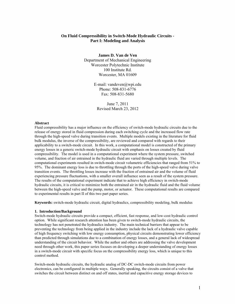
where D is the volumetric displacement of the hydraulic motor and ω is the angular velocity of the motor. The flow rate through the check valve is modeled using the orifice equation, with flow occurring when the pressure drop across the valve exceeds the cracking pressure as:

2 for

0 for

D check tank switch tank switch crack

check

tank switch crack

C A P P P P PQ

P P P

(15)

where CD is the discharge coefficient, Acheck is the cross-sectional area of the open check valve, ρ is the mass density of the fluid, and Ptank is the pressure of the reservoir. Note that the check valve is assumed to open instantaneously. Finally, the flow rates through the ports of the high-speed valve are also described by the orifice equation with a variable area as:

8

,2

valve P A D P A high switchQ C A P P (16)

,

2 for 0

2 for 0

D T A tank switch tank switch

valve T A

D T A switch tank tank switch

C A P P P PQ

C A P P P P

(17)

where APA, ATA is the cross-sectional area of the PA and TA connections in the high-speed valve respectively and Phigh is the accumulator pressure. Note that the two cases are required in the evaluation of the TA flow rate to account for flow reversal. The variable orifice areas of the high-speed valve ports are modeled as circular cross-sections that are partially obstructed by a moving plane, as illustrated in Figure 3.

Figure 3. Geometry of the port areas created by circular orifices that are partially obstructed by the moving spool, represented as a moving plane. Note, the positive direction of lT and lP is towards the open area of the moving plane.

Without further knowledge, the moving plane is assumed to translate at a constant velocity, which is set by the valve transition time. Based on the geometry presented in Figure 3, the axial position of the moving plane, s, for any time, t, can be expressed in pseudo-code as:

,

,

if mod

2if 2

elseif mod

else 2

elseif mod

2if 0

else

else 0

d P prev

P TP T prev

Pon

P T

on d T prev

P Tprev

T

t T t s s

r r ts r r s s

tt T t

s r ry t

t T t t s s

r r ts s s

t

s

(18)

where T is the switching period defined as 1/freq, td,P and td,T are the time delay between sending a signal to the valve and movement of the valve spool during transition to PA and TA respectively, ton is the time the command signal is sent for the valve to be in the PA position defined as T*duty, yprev is the position of the moving plane at the previous time step, Δt is the time step, and rP and rT are the radius of the P port and T port respectively. The modulo function is used to evaluate the time relative to the switching period. The complexity of the second evaluation is driven by the need to accommodate overlapping on and off transition periods. From the axial position of the moving plane, the axial position of the open area relative to the center of each circular orifice, lP and lT, is described by:

9

if 2

else2

T TT

P P

T T

P P T

l s rs r

l r

l r

l r r s

(19)

Finally, the orifice area of the valve is described by:

2 2

2 22 2 2 2 2

0

2 22 2 2 2

2 arcsin for 0

( )

arcsin for 0

r l r lr y l dy r l r l l

rA l

r lr r l r l l

r

(20)

where the appropriate subscript is placed on A, r, and l to calculate the cross-sectional area for the pressure and tank port. Plots of the valve command, linear valve displacement, and orifice areas of the valve ports as a function of time for a duty cycle of 60% are provide in Figure 4.

Figure 4. On-off valve command, spool displacement, and orifice areas as a function of time during two switching periods with a duty cycle of 60%.

For commercially available valves, the internal orifice areas and the discharge coefficients are typically not provided. Instead, a plot is typically provided of the fully open pressure drops as a function of flow rate.

10

By selecting data points from the pressure-drop plot of the valve used in part II of this paper series [6], a value for CD*A for both the pressure and tank ports can be calculated for use in the above equations. Note that this method ignores the influence of geometry and flow conditions on the discharge coefficient by simplying creating lumped values for the fully open CD*A values. To determine the pressure in the switched volume, the flow Eqns. (14)-(17) are substituted into Eqn. (12), which is then numerically integrated. Equations (15)-(17) can be rearranged to solve for the pressure drop across both ports of the high-speed valve and the check valve. The total energy loss due to throttling flow across the ports in the high-speed valve and the check valve is described as:

, , , ,throttle valve P A valve P A valve T A valve T A check checkE P Q P Q P Q dt . (21)

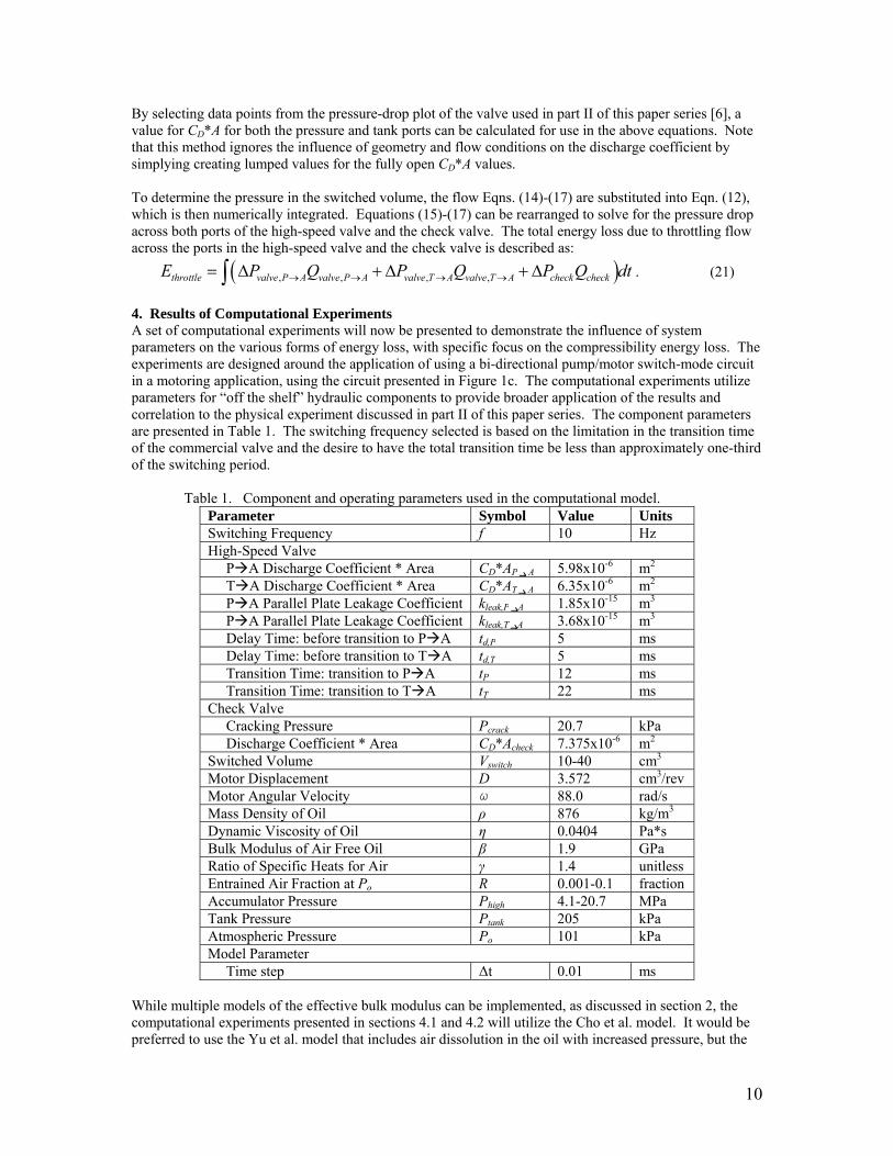
4. Results of Computational Experiments A set of computational experiments will now be presented to demonstrate the influence of system parameters on the various forms of energy loss, with specific focus on the compressibility energy loss. The experiments are designed around the application of using a bi-directional pump/motor switch-mode circuit in a motoring application, using the circuit presented in Figure 1c. The computational experiments utilize parameters for “off the shelf” hydraulic components to provide broader application of the results and correlation to the physical experiment discussed in part II of this paper series. The component parameters are presented in Table 1. The switching frequency selected is based on the limitation in the transition time of the commercial valve and the desire to have the total transition time be less than approximately one-third of the switching period.

Table 1. Component and operating parameters used in the computational model. Parameter Symbol Value Units Switching Frequency f 10 Hz High-Speed Valve PA Discharge Coefficient * Area CD*AP A 5.98x10-6 m2 TA Discharge Coefficient * Area CD*AT A 6.35x10-6 m2 PA Parallel Plate Leakage Coefficient kleak,PA 1.85x10-15 m3 PA Parallel Plate Leakage Coefficient kleak,TA 3.68x10-15 m3 Delay Time: before transition to PA td,P 5 ms Delay Time: before transition to TA td,T 5 ms Transition Time: transition to PA tP 12 ms Transition Time: transition to TA tT 22 ms Check Valve Cracking Pressure Pcrack 20.7 kPa Discharge Coefficient * Area CD*Acheck 7.375x10-6 m2 Switched Volume Vswitch 10-40 cm3 Motor Displacement D 3.572 cm3/rev Motor Angular Velocity ω 88.0 rad/s Mass Density of Oil ρ 876 kg/m3 Dynamic Viscosity of Oil η 0.0404 Pa*s Bulk Modulus of Air Free Oil β 1.9 GPa Ratio of Specific Heats for Air γ 1.4 unitless Entrained Air Fraction at Po R 0.001-0.1 fraction Accumulator Pressure Phigh 4.1-20.7 MPa Tank Pressure Ptank 205 kPa Atmospheric Pressure Po 101 kPa Model Parameter Time step Δt 0.01 ms

While multiple models of the effective bulk modulus can be implemented, as discussed in section 2, the computational experiments presented in sections 4.1 and 4.2 will utilize the Cho et al. model. It would be preferred to use the Yu et al. model that includes air dissolution in the oil with increased pressure, but the

11

experimentally determined c1 coefficient required for this model is unknown, preventing accurate implementation. In appendix A, the author presents results of implementing each of the bulk modulus models into the circuit simulation. 4.1 Results of the Control Case During a single switching period, the flow rate through both ports of the high-speed valve and check valve vary significantly due to both the switching action and the change in density of the hydraulic fluid in the switched volume as a function of pressure, as defined by the bulk modulus. While the pressure at the inlet side of all of the valve ports remains constant at the tank or accumulator pressure, the fluctuating pressure in the switched volume creates a varying pressure drop across all valve ports. The relationship between the pressure in the switched volume, the flow rate through each valve port and the corresponding power loss due to throttling across the valves are presented in Figure 5. Because the check valve flutters open and closed due to the assumption of opening instantaneously, a 20-point moving average is applied to the check valve flow rate. Note that these plots are for a relatively “stiff” switched volume, meaning that the effective bulk modulus of the hydraulic fluid is high due to a low air entrainment of 1% and a small switched volume of 10 cm3. The system pressure for this case is 20.7 MPa.

12

Figure 5. Pressure in the switched volume and flow rate and power loss through the on-off valve and the check valve as a function of time during two switching periods at a duty cycle of 60%, a system pressure of 20.7 MPa, a switched volume of 10 cm3, and air entrainment of 1%.

The time delays in the motion of the high-speed valve in Figure 5 corresponds to the same 60% duty cycle signal and valve open area in Figure 4. When the high-speed valve begins to transition to PA, near a time 0.112 seconds, a large pulse in the flow rate occurs, resulting in an increase in the pressure and corresponding density of the fluid in the switched volume. Because this fluid pulse occurs when the valve is only partially open, producing a large pressure drop, this event creates a large spike in power loss, seen in the fourth subplot of Figure 5. Note that this power loss spike is orders of magnitude greater than the fully-open throttling power loss. When the high-speed valve transitions to TA, near a time of 0.175

13

seconds, fluid from the switched volume flows backwards through the valve to tank, resulting in a spike in the throttling energy loss, as seen in the fifth subplot. The check valve minimizes the pressure drop across the high-speed valve during when the TA port is opening or closing. For example, when the TA port is closing (near 0.21s), the motor is drawing flow, some of which passes through the TA port and the rest of which passes through the check valve. Note that the power loss associated with throttling across the check valve is significantly lower than the spikes created by the previously described transition events. For reference, the throttling energy loss through the PA port during one second of operation at the above conditions is 40.62 Joules, the throttling energy loss through the TA port (both directions) is 0.58 Joules, the throttling energy loss through the check valve is 0.11 Joules, and 642 Joules of energy reaches the hydraulic motor. Beyond energy losses due to fluid throttling, another significant energy loss is the internal valve leakage. As the valve leakage is greater across the PA port due to the higher pressure differential, the leakage energy loss is duty cycle dependent. Because the leakage across the valve is a function of the pressure in the switched volume, the energy loss due to leakage is also a function of the “stiffness” of the switched volume as this drives the rate of pressure change. For reference, at the above operating conditions, the leakage energy loss during one second of operation is 6.71 Joules across the PA port and 0.12 Joules across the TA port. 4.2 Results of Varying Entrained Air, Switched Volume, and System Pressure To explore the influence of entrained air content, switched volume, and system pressure on the throttling losses and internal leakage losses, a series of computational experiments were run. For these experiments, three levels of each factor were created with pressure factors of 4.1 MPa, 6.9 MPa, and 20.7 MPa, switched volume factors of 10 cm3, 20 cm3, and 40 cm3, and entrained air at atmospheric pressure of 0.1%, 1%, and 10%. The results of these experiments are presented in Table 2. Note, the energy losses associated with actuating the valve, which include inertial forces and viscous friction are not modeled as they are highly dependent of the specific valve design. For this reason, the volumetric efficiency is reported, which is the energy reaching the hydraulic motor divided by the sum of the energy to the motor, the internal leakage, and throttling energy losses. Further note that the TA throttling loss is defined as throttling when flow passes from tank to the switched volume while the AT throttling loss occurs during a flow reversal from the switched volume to tank. Finally, the TA leakage losses were not included in the table due to their small magnitude, ranging from 0.008 Joules to 0.13 Joules.

14

Table 2. Energy losses, energy to the hydraulic motor, and volumetric efficiency of the switch-mode circuit. Note that the reported energy is for one second of operation. Input Parameters Energy Losses

Energy to Motor

Volume Efficiency

System Press

Switch Volume

Entrain Air

PA Throt

TA Throt

AT Throt

Check Throt

PA Leak

(MPa) (cm3) (fract) (J) (J) (J) (J) (J) (J) (%)

4.1

10 0.001 5.62 0.20 0.00 0.14 0.25 117.8 94.80 0.01 8.03 0.24 0.00 0.13 0.25 117.2 92.95

0.1 27.90 0.22 0.34 0.07 0.24 115.9 79.99

20 0.001 6.22 0.22 0.00 0.14 0.25 117.8 94.34 0.01 10.83 0.24 0.00 0.11 0.25 117.1 90.93

0.1 49.24 0.17 1.58 0.06 0.23 115.5 69.15

40 0.001 7.58 0.23 0.00 0.13 0.25 118.0 93.33 0.01 16.35 0.23 0.08 0.09 0.24 117.1 87.16

0.1 91.46 0.08 5.32 0.04 0.22 114.1 53.97

6.9

10 0.001 8.29 0.20 0.00 0.13 0.73 205.5 95.32 0.01 12.72 0.24 0.00 0.12 0.73 204.6 93.37

0.1 49.08 0.22 0.59 0.07 0.71 202.0 79.72

20 0.001 10.01 0.22 0.00 0.13 0.73 205.8 94.57 0.01 18.36 0.24 0.02 0.11 0.72 204.6 91.02

0.1 88.47 0.17 2.60 0.06 0.69 201.2 68.46

40 0.001 13.77 0.23 0.07 0.11 0.72 206.6 92.97 0.01 29.48 0.23 0.41 0.09 0.71 205.0 86.63

0.1 166.01 0.08 8.55 0.04 0.65 199.4 53.12

20.7

10 0.001 26.76 0.20 0.22 0.12 6.72 644.7 94.06 0.01 40.62 0.24 0.34 0.11 6.71 642.3 92.15

0.1 159.53 0.21 2.62 0.07 6.59 633.3 78.29

20 0.001 41.58 0.22 3.01 0.11 6.58 648.1 91.77 0.01 67.49 0.23 3.61 0.09 6.56 644.9 88.41

0.1 297.18 0.16 11.11 0.05 6.42 631.9 66.29

40 0.001 70.12 0.23 14.33 0.10 6.40 652.3 86.99 0.01 119.41 0.23 16.02 0.08 6.38 647.8 81.35

0.1 567.69 0.08 34.91 0.04 6.18 628.8 50.55 A few general trends are observed in Table 2. First, as expected, an increase in pressure results in increased throttling and leakage loss; this influence is especially apparent on the PA and AT throttling losses, which become quite sizeable at higher pressures. However, the overall influence of pressure on the volumetric efficiency is quite small, where the low or medium pressures generally produce the highest efficiency. Second, it is noted that an increase in the entrained air or the switched volume result in an increase in the dominant PA and AT throttling energy losses, creating a corresponding decrease in hydraulic efficiency. The influence of these factors on the three forms of throttling loss is presented in Figure 6. Note that the y-axis of the subplots is the non-dimensional energy, defined as the throttling energy divided by the energy reaching the motor. The combined influence of the factors on the volumetric efficiency can be further visualized in Figure 7.

15

0 1 2 3 4 5 6 7 8 9 100

0.2

0.4

0.6

0.8

1

Entrained Air (%)

Ene

rgy

Fra

ctio

n (u

nitl

ess)

P->A Throttling Energy Divided by Energy to Motor

10 cc20 cc

40 cc

4.1 MPa

6.9 MPa20.7 MPa

0 1 2 3 4 5 6 7 8 9 100

0.5

1

1.5

2

2.5x 10

-3

Entrained Air (%)

Ene

rgy

Fra

ctio

n (u

nitl

ess)

T->A Throttling Energy Divided by Energy to Motor

0 1 2 3 4 5 6 7 8 9 100

0.02

0.04

0.06

Entrained Air (%)

Ene

rgy

Fra

ctio

n (u

nitl

ess)

A->T Compressibility Throttling Energy Divided by Energy to Motor

Figure 6. Influence of the entrained air, system pressure, and switched volume on the three forms of throttling energy loss. To scale the results for comparison purposes, the y-axes are the throttling energy divided by the energy reaching the hydraulic motor.

16

0 1 2 3 4 5 6 7 8 9 1050

55

60

65

70

75

80

85

90

95

100

Entrained Air (%)

Eff

icie

ncy

(%)

Volumetric Efficiency vs. Air Entrainment, Switched Volume, and Pressure

10 cc20 cc

40 cc

4.1 MPa

6.9 MPa20.7 MPa

Figure 7. Volumetric efficiency as a function of entrained air, switched volume, and system pressure.

The significant increase in PA and AT throttling energy loss with increased switched volume and entrained air is a direct result of the “stiffness” of the fluid in the switched volume. As the “stiffness” decreases, as results from a decrease in the bulk modulus and an increase in the volume, the change in mass of the fluid in the switched volume increases during each switching period. This change in mass results from rapid flow primarily through partially open ports of the high-speed valve during the transition events, resulting in the high energy losses. This behavior can be visualized in Figure 8, plots of the pressure in the switched volume, flow rates into the switched volume, and corresponding throttling energy losses for conditions of 21 MPa, 40 cm3 volume, and 10% air entrainment. Note the significant negative flow through the TA port near a time of 0.175 seconds. This period when fluid is flowing from the switched volume to tank is the AT throttling loss. For this low “stiffness” condition, the maximum power of the AT throttling loss is of the same order of magnitude as the PA throttling loss.

17

Figure 8. Pressure in the switched volume, flow rates through the three ports into the switched volume, and corresponding throttling energy losses for a duty cycle of 60%, system pressure of 20.7 MPa, a switched volume of 40 cm3, and air entrainment of 10%.

5. Discussion The results of the simulation cases demonstrate the influence of operating parameters on energy losses in the switch-mode circuit, particularly the compressibility of the fluid in the switched volume. As seen in Figure 7, the volumetric efficiency decreases with increasing entrained air, switched volume, and to a smaller extent, pressure. This section contains a discussion of the fluid behavior in the switched volume during valve transition, the energy losses and volumetric efficiency of the circuit as a function of the “stiffness” of the fluid in the switched volume, and the predicted volumetric efficiency as a function of the bulk modulus model utilized in the computational model.

18

The throttling energy losses are significantly larger than the leakage losses for all simulation cases. Of the throttling losses, the throttling across the PA port dominates, with the majority of this energy loss occurring during a spike in flow when the PA port begins to open. When this flow pulse occurs, which is around 0.112 seconds in Figure 5 and Figure 8, the port is only partially open, creating a large pressure drop and corresponding large power loss. The second largest energy loss for the majority of the cases is AT throttling. This throttling loss is characterized by a flow reversal, where fluid from the switched volume flows through the high-speed valve to tank; it is not to be confused with the TA throttling loss where the flow direction through the TA port is positive. The majority of the AT throttling loss also occurs in one flow pulse, which is around 0.175 seconds in Figure 5 and Figure 8. Both the PA and AT throttling losses are primarily due to the compressibility of the fluid in the switched volume, and thus increase with the entrained air fraction, volume, and pressure. However, the influence of pressure on these two throttling loss terms on the volumetric efficiency, particularly the PA throttling loss, is obfuscated by the increase in energy of the motor due to the increase in pressure. The throttling loss due to a positive flow from the tank port to the switched volume behaves quite differently than the previously discussed throttling losses. The TA throttling loss, which occurs when there is flow into the switched volume from tank, is generally small compared to the other throttling terms. When the pressure in the switched volume plus the check valve cracking pressure is less than the tank pressure the check valve is also open, sharing a portion of the flow from tank to the switched volume. When this positive pressure differential occurs and the TA port is opening or closing, the flow through the check valve increases, preventing a high flow rate across a small area. The energy loss due to the TA throttling actually decreases slightly with increasing entrained air, switched volume, and pressure due to reverse flow occupying a longer portion of the time that the T and A ports are connected. The difference in the duration of the reverse flow is apparent when comparing the negative flow pulses in the third subplots of Figure 5 and Figure 8. The energy losses due to leakage across the ports of the high-speed valve were significantly lower than the throttling losses for all simulation cases. Because the leakage is modeled as laminar flow between parallel plates, the leakage flow rate increases linearly with pressure differential and thus the energy loss across the PA port increases with pressure squared. More subtle was the change in PA leakage with air entrainment and switched volume. As the air entrainment and switched volume increased, decreasing the “stiffness” of the fluid in the switched volume, the PA leakage energy loss decreased. The reason for this decrease is that the average pressure drop across the closed PA port decreased as the lower “stiffness” switched volume increased the duration of the pressure drop when the TA port is opening. The results of the TA leakage were not included in Table 2 and will not be discussed further because of the small contribution to the overall energy loss. It does need to be noted that the leakage rate is a function of the duty cycle and the PA leakage loss becomes more dominant with decreasing duty cycle. 6. Conclusion In this paper, a computational model of a switch-mode circuit for a virtually variable displacement bi-directional pump/motor was presented with primary purpose of studying the compressibility energy loss. By modeling the pressure in the switched volume as a function of the bulk modulus and flow rate through the two ports of the on-off and check valves, unique behavior was discovered. By systematically varying operating parameters, trends in energy loss as a function of the “stiffness” of the fluid in the switched volume were revealed. Finally, the importance of an accurate bulk modulus model is apparent through the prediction of volumetric efficiency across the full duty cycle range utilizing different bulk modulus models. This model is experimentally verified in part II of this paper series [6]. Of the 27 simulation cases, the peak volumetric efficiency of 95.3% was found at a switched volume of 10 cm3, air entrainment of 0.1% and a pressure of 6.9 MPa. While the influence of the pressure on volumetric efficiency was mixed at the two lower levels and a decrease in efficiency at the highest pressure level, the influence of entrained air and volume were quite clear. The volumetric efficiency was found to improve with decreasing switched volume and decreasing air entrainment, which both lead to a decrease in “stiffness” of the fluid in the switched volume. The nature of the energy loss associated with the fluid compressibility is that every time the switched volume is connected to the pressure port, the fluid density

19

increases, storing energy in fluid compression. When the switched volume is connected to the tank port, the energy stored in the fluid compression is released through a reverse flow to tank. The compressibility energy loss increases linearly with the switching frequency, and can become quite problematic for high frequency systems. The consequences of this finding to the design of switch-mode systems is that minimizing air entrainment in the hydraulic fluid and minimizing the switched volume are critical to a high efficiency system. The air entrained in the hydraulic fluid can be minimized through good reservoir design including: returning all lines below the fluid level, placing the suction port as far away from the return lines as possible, and utilizing an angled screen over the suction port to encourage entrained air to rise to the surface [8]. More aggressive means of reducing air entrainment include degassing the hydraulic fluid by placing it in a vacuum and then sealing the hydraulic circuit or adding a deaerator in the hydraulic circuit. To minimize the switched volume, the high-speed valve and check valve must be placed as close to the pump, motor, or hydraulic actuator as possible and the fluid volume between these components must be minimized. Ideally, the valves and actuator can be integrated into a single manifold to further reduce the fluid volume. Four different bulk modulus models were specifically discussed in the body and appendix of this paper, and additional models exist in the literature. The primary differences between existing models include the assumption of adiabatic or isothermal compression of entrained air, accounting for the change in the density of the hydraulic fluid with pressure, and accounting for entrained air dissolving into the hydraulic fluid with increased pressure. However, additional factors that influence the effective bulk modulus are not included in the existing models. First, the influence of temperature on both the bulk modulus of air-free hydraulic fluid, which decreases with increasing temperature [8], and on gas solubility, are not included. This is especially important for mobile hydraulic applications that operate at extreme ambient temperatures. Second, the existing models do not account for the rate of pressure change, which influences both the assumption of isothermal or adiabatic entrained air compression and the rate of gas dissolution and release from solution. As the bulk modulus is critical to switch-mode circuits, an area for future work is including these additional factors into a comprehensive bulk modulus model. The modeling work in this paper focused on a bi-directional pump/motor circuit operated in motoring mode. While a purely motor circuit, depicted in Figure 1b, would minimize the influence of the energy loss due to compressibility, as the compressed fluid is not released to tank, the presented work is more generally applicable to generic switch-mode circuits. The bi-directional circuit is important to study due to the current emphasis on system efficiency, which can be drastically improved with a switch-mode circuit that allows reversed flow for energy regeneration by energy storage in the hydraulic accumulator. 7. References [1] Tu, H. C., Rannow, M., Wang, M., Li, P., Chase, T., and Van de Ven, J., 2011, "Design, Modeling, and Validation of a High-Speed Rotary PWM on/Off Hydraulic Valve," Journal of Dynamic Systems, Measurement, and Control,(Under Review). [2] Van de Ven, J. D., and Katz, A., 2011, "Phase-Shift High-Speed Valve for Switch-Mode Control," Journal of Dynamic Systems, Measurement, and Control, 133(1). [3] Batdorff, M. A., and Lumkes, J. H., 2006, "Virtually Variable Displacement Hydraulic Pump Including Compressability and Switching Losses," ASME International Mechanical Engineering Congress and Exposition, Chicago, IL, pp. 57-66. [4] Lumkes, J. H., Batdorff, M. A., and Mahrenholz, J. R., 2009, "Model Development and Experimental Analysis of a Virtually Variable Displacement Pump System," International Journal of Fluid Power, 10(3), pp. 17-27. [5] Tomlinson, S. P., and Burrows, C. R., 1992, "Achieving a Variable Flow Supply by Controlled Unloading of a Fixed-Displacement Pump," Journal of Dynamic Systems, Measurement, and Control, 114, pp. 166-171. [6] Van de Ven, J. D., 2011, "On Fluid Compressibility in Switch-Mode Hydraulic Circuits - Part II: Experimental Results," Journal of Dynamic Systems, Measurement, and Control,(under review). [7] Watton, J., 1989, Fluid Power Systems: Modeling, Simulation, Analog and Microcomputer Control, Prentice Hall, New York.

20

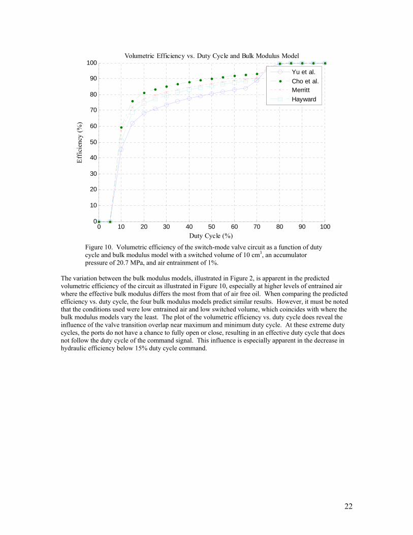
[8] Totten, G. E., Webster, G. M., and Yeaple, F. D. (2000). "Physical Properties and Their Determination." In: Handbook of Hydraulic Fluid Technology, G. E. Totten, ed., Marcel Dekker, Inc., New York. [9] Akers, A., Gassman, M., and Smith, R., 2006, Hydraulic Power Systems Analysis, Taylor & Francis, Boca Raton. [10] Merritt, H. E., 1967, Hydraulic Control Systems, John Wiley & Sons, New York. [11] Watton, J., 2007, Modelling, Monitoring and Diagnostic Techniques for Fluid Power Systems, Springer, London. [12] Cho, B.-H., Lee, H.-W., and Oh, J.-S., 2002, "Estimation Technique of Air Content in Automotic Transmission Fluid by Measuring Effective Bulk Modulus," International Journal of Automotive Technology, 3(2), pp. 57-61. [13] Yu, J., Chen, Z., and Lu, Y., 1994, "The Variation of Oil Effective Bulk Modulus with Pressure in Hydraulic Systems," Journal of Dynamic Systems, Measurement, and Control, 116, pp. 146-150. [14] Ruan, J., and Burton, R., 2006, "Bulk Modulus of Air Content Oil in a Hydraulic Cylinder," ASME International Mechanical Engineering Congress and Exposition, 15854, Chicago, IL. [15] Tu, H. C., Rannow, M., Van de Ven, J., Wang, M., Li, P., and Chase, T., 2007, "High Speed Rotary Pulse Width Modulated on/Off Valve," Proceedings of the ASME International Mechanical Engineering Congress, Seattle, WA, pp. 42559. [16] Brown, F. T., Tentarelli, S. C., and Ramachandran, S., 1988, "A Hydraulic Rotary Switched-Inertance Servo-Transformer," Journal of Dynamic Systems, Measurement, and Control, 110(2), pp. 144-150. [17] Cyphelly, I., and Langen, H. J., 1980, "Ein Neues Energiesparendes Konzept Der Volumenstromdosierung Mit Konstantpumpen," Aachener Fluidtechnisches Kolloquium, pp. 42-61. [18] Royston, T., and Singh, R., 1993, "Development of a Pulse-Width Modulated Pneumatic Rotary Valve for Actuator Position Control," Journal of Dynamic Systems, Measurement, and Control, 115, pp. 495-505. 8. Appendix: Investigations into Selection of Bulk Modulus Model: The results generated in this paper solely used the Cho et al. effective bulk modulus model. This appendix will explore the predicted hydraulic efficiency using all of the bulk modulus models discussed in section 2. The primary differences between the bulk modulus models are adiabatic vs. isothermal assumption, accounting for hydraulic fluid density change with pressure, and accounting for air dissolution. These differences can be observed in Figure 9, a plot of the predicted hydraulic efficiency using each model as a function of the entrained air. An estimate has been made for the gas dissolution coefficient, c1, of -9.307x10-6, for the Yu et al. model based on their experimental work [13]. Note that the other system parameters are the same as the control used in section 4.1, a switched volume of 10 cm3, a system pressure of 20.7 MPa, and a duty cycle of 60%.

21

0 1 2 3 4 5 6 7 8 9 1020

30

40

50

60

70

80

90

100

Entrained Air (%)

Eff

icie

ncy

(%)

Volumetric Efficiency vs. Entrained Air and Bulk Modulus Model

Yu et al.

Cho et al.Hayward

Merritt

Figure 9. Volumetric efficiency as a function of entrained air utilizing different bulk modulus models with a switched volume of 10 cm3, an accumulator pressure of 20.7 MPa, and a duty cycle of 60%.

The results presented in the body of the paper used a fixed duty cycle of 60%, while focusing on the influence of the other process parameters. The combined influence of the bulk modulus model and the duty cycle on the hydraulic efficiency is presented in Figure 10. Model parameters were again set at the control conditions of a switched volume of 10 cm3, a system pressure of 20.7 MPa, and an entrained air content of 1%.

22

0 10 20 30 40 50 60 70 80 90 1000

10

20

30

40

50

60

70

80

90

100

Duty Cycle (%)

Eff

icie

ncy

(%)

Volumetric Efficiency vs. Duty Cycle and Bulk Modulus Model

Yu et al.

Cho et al.Merritt

Hayward

Figure 10. Volumetric efficiency of the switch-mode valve circuit as a function of duty cycle and bulk modulus model with a switched volume of 10 cm3, an accumulator pressure of 20.7 MPa, and air entrainment of 1%.

The variation between the bulk modulus models, illustrated in Figure 2, is apparent in the predicted volumetric efficiency of the circuit as illustrated in Figure 10, especially at higher levels of entrained air where the effective bulk modulus differs the most from that of air free oil. When comparing the predicted efficiency vs. duty cycle, the four bulk modulus models predict similar results. However, it must be noted that the conditions used were low entrained air and low switched volume, which coincides with where the bulk modulus models vary the least. The plot of the volumetric efficiency vs. duty cycle does reveal the influence of the valve transition overlap near maximum and minimum duty cycle. At these extreme duty cycles, the ports do not have a chance to fully open or close, resulting in an effective duty cycle that does not follow the duty cycle of the command signal. This influence is especially apparent in the decrease in hydraulic efficiency below 15% duty cycle command.