On First-Order Hyperbolic Partial Differential Equations ...ruan/MyPapers/Kang_Huo...In populations...

On First-Order Hyperbolic Partial Differential Equationswith Two Internal Variables Modeling Population

Dynamics of Two Physiological Structures∗

Hao Kang, Xi Huo and Shigui Ruan

Department of Mathematics, University of Miami, Coral Gables, FL 33146, USA

April 25, 2020

Abstract

In this paper we develop fundamental theories for a scalar first-order hyperbolic par-tial differential equation with two internal variables which models single species populationdynamics with two physiological structures such as age-age, age-maturation, age-size, andage-stage. Classical techniques of treating structured models with a single internal variableare generalized to study the double physiologically-structured model. First the semigroupis defined based on the solutions and its infinitesimal generator is determined. Then thecompactness of solution trajectories are established. Finally spectrum theory is employed toinvestigate stability of the zero steady state and asynchronous exponential growth of solu-tions is studied when the zero steady state is unstable.

Key words: Physiological structure; semigroup theory; infinitesimal generator; spectrum the-ory; asynchronous exponential growth.

AMS subject classifications: 35L04, 92D25, 47A10

Contents

1 Introduction 2

2 The Semigroup 42.1 A Priori Estimate . . . . . . . . . . . . . . . . . . . . . . . . . . . . . . . . . . . . . . 5

2.2 Existence and Uniqueness of Solutions . . . . . . . . . . . . . . . . . . . . . . . . . 6

2.3 Semigroup Generated by the Solution Flow . . . . . . . . . . . . . . . . . . . . . . . 8

2.4 Solutions of the Initial-Boundary Value Problem . . . . . . . . . . . . . . . . . . . . 12

3 The Infinitesimal Generator 13

4 Compactness of Solution Trajectories 18

5 Spectrum Analysis 235.1 Point Spectrum and Stability Analysis . . . . . . . . . . . . . . . . . . . . . . . . . . 24

5.2 Asynchronous Exponential Growth . . . . . . . . . . . . . . . . . . . . . . . . . . . 33

5.3 Asymptotic Behavior for R0 = 1 . . . . . . . . . . . . . . . . . . . . . . . . . . . . . 35

∗Research was partially supported by National Science Foundation (DMS-1853622).

1

Annali di Matematica Pura ed Applicata (accepted)

2

6 Discussion 36

A Appendix 38

References 41

1 Introduction

In populations dynamics, structured models bridge the gap between the individual leveland the population level and allow us to study the dynamics of populations from properties ofindividuals or vice versa (Metz and Diekmann [40]). In order to parametrize the state of individ-uals as well as to distinguish individuals from one another, we usually take their physiologicalconditions or physical characteristics such as age, maturation, size, stage, status, location, andmovement into consideration and determine their birth, growth and death rates, interactionswith each other and with environment, infectivity, and so on. The goal of studying structuredpopulation models is to understand how these physiological conditions or physical characteris-tics affect the dynamical properties of these models and thus the outcomes and consequences ofthe biological and epidemiological processes (Magal and Ruan [34]).

Age structure is the most important characteristic in population dynamics. It is well-knownfor a long time that the age-structure of a population affects the nonlinear dynamics of thespecies in ecology and the transmission dynamics of infectious diseases in epidemiology. Inmodeling specific diseases, the age could be chronological age (the age of the population), infec-tion age (the time elapsed since infection), recovery age (the time elapsed since the last infection),class age (the length of time in the present group), etc. The theory of age-structured models hasbeen well-developed, we refer to the classical monographs of Anita [1], Iannelli [23], Inaba [26],and Webb [52] on this subject. Models with other physiological structures, such as size and stage,have also been extensively studied in the literature (Barfield et al. [3], Cushing [7], Ebenman andPersson [17], Manly [36], Metz and Diekmann [40]).

There are some models taking into account the combined effects of two age characteristics.Hoppensteadt [22] proposed a double age-structured epidemic model for a population con-sisted of susceptible, infectious, quarantined infectious, and immune classes by keeping trackof the chronological ages of the individuals as well as their class ages (i.e., the length of timesince entering their present state). Existence and uniqueness of solutions to the model wereconsidered. In order to determine the likely success of isolating symptomatic individuals andtracing and quarantining their contacts, Fraser et al. [19] studied a double age-structured modelinvolving individuals who were infected time τ ago by people who themselves were infectedtime τ′ ago. They concluded direct estimation of the proportion of asymptomatic and presymp-tomatic infections is achievable by contact tracing and should be a priority during an outbreakof a novel infectious agent. Kapitanov [29] considered the coinfection of HIV and tuberculosisin which each disease progresses through several stages. He suggested modeling these stagesthrough a time since-infection tracking transmission rate function and introduced a double age-structured model. By incorporating the chronological ages of the individuals into the Kermackand McKendrick’s original infection-age structured endemic model, Inaba [25] developed a dou-ble age-structured susceptible-infectious-recovered model and studied some basic properties ofthe model. Burie et al. [6] investigated an age and infection age structured model for the propa-gation of fungal diseases in plants and analyzed the asymptotic behavior of the model. Larocheand Perasso [33] studied a generic epidemic model structured by age and, for infected, the timeremaining before the end of the incubation where they show detectable clinical signs. Popula-tion dynamical models with age and size structures (Sinko and Streifer [44], Webb [55]), age and

3

maturation structures (Dyson et al. [15,16]), age and stage structures (McNair and Goulden [39],Matucci [38]), and age and an aggregated variable (Doumic [13]) have also been proposed andstudied by many researchers.

Though many epidemic and populations models with two physiological structures have beenproposed in the literature (as mentioned above), there are very few theoretical studies on the fun-damental properties of such equations. By considering the property of the disease-free steadystate of a susceptible-infectious-recovered model with chronological and class ages, Inaba [25]obtained a scalar equation with two age structures and provided some analysis of the model, in-cluding global stability of the disease-free steady state, using the strongly continuous semigrouptheory. Webb [53] investigated a scalar structured population model with nonlinear boundaryconditions in which individuals are distinguished by age and another physical characteristic andproved that populations structured by two internal variables converge to stable distributions.

Motivated by the studies of Inaba [25] and Webb [53], in this paper we aim to developfundamental results and theories for a scalar equation with two physiological structures andto generalize the techniques in treating single age-structured models (Iannelli [23], Inaba [26],Webb [51, 52]) to study structured models with two internal variables. Consider the followingfirst-order hyperbolic partial differential equation with two internal variables a and a′ (whichmodels single species population dynamics with two physiological structures)

∂u(t, a, a′)∂t

+∂u(t, a, a′)

∂a+

∂u(t, a, a′)∂a′

= −µ(a, a′)u(t, a, a′), t > 0, (a, a′) ∈ (0, a+)× (0, a+) (1.1)

under the initial condition

u(0, a, a′) = φ(a, a′), a ∈ (0, a+), a′ ∈ (0, a+) (1.2)

and boundary conditions

u(t, 0, a′) =∫ a+

0

∫ a+

0β(a′, a, s)u(t, a, s)dads, t > 0, a′ ∈ (0, a+), (1.3)

u(t, a, 0) =∫ a+

0

∫ a+

0β′(a, s, a′)u(t, s, a′)dsda′, t > 0, a ∈ (0, a+). (1.4)

Here u(t, a, a′) denotes the density of a population at time t with age a and another characteristica′ (age, size, maturation, stage, etc.), the function φ represents the initial distribution of thepopulation with respect to age a and another physiological characteristic a′. µ(a, a′) denotes themortality rate of the population at age a with characteristic a′. Boundary condition (1.3) accountsfor the input at time t of individuals of age 0 with characteristic a′ and boundary condition (1.4)describes the input at time t of individuals of age a with characteristic a′ at level 0. Here a+

represents the maximum age or characteristic and could be infinity.By using semigroup theory, we study the basic properties and dynamics of model (1.1) un-

der the initial condition (1.2) and boundary conditions (1.3)-(1.4), including the solution flowu(t, a, a′) and its semigroup S(t)t≥0 with infinitesimal generator A. Moreover, we establishthe compactness of the solution trajectories, analyze the spectrum of A, investigate stability ofthe zero equilibrium, and discuss the asynchronous exponential growth of the solutions whenthe zero equilibrium is unstable. We study the initial-boundary value problem in the two cases:a+ < ∞ and a+ = ∞. First, we show that for a+ < ∞ the semigroup S(t)t≥0 with infinitesimalgenerator A is eventually compact, while for a+ = ∞ the semigroup S(t)t≥0 is quasi-compact.Next, we study the existence and uniqueness of the principle and simple eigenvalue and spectralbound of A under extra assumptions (see Assumption 2.1(iii)’ and (5.7)) for a+ = ∞. Finally, weestablish the same threshold dynamics for these two cases.

4

2 The Semigroup

In this section we investigate the existence and uniqueness of solutions to the initial-boundaryvalue problem (1.1)-(1.4) via theory of integral functions. By using the method of characteristiclines we obtain the following expression for the density u(t, a, a′) (the computation details aregiven in Section 6)

u(t, a, a′) =

φ(a− t, a′ − t)e−

∫ t0 µ(s−t+a,s−t+a′)ds, t < a < a′ < a+ or t < a′ < a < a+

u(t− a, 0, a′ − a)e−∫ a

0 µ(s,s+a′−a)ds, a < t < a′ < a+ or a < a′ < t, a < a′ < a+

u(t− a′, a− a′, 0)e−∫ a′

0 µ(s+a−a′,s)ds, a′ < a < t, a′ < a < a+ or a′ < t < a < a+.

(2.1)

Assumption 2.1. Assume that

(i) β, β′ : [0, a+)× [0, a+)× [0, a+) → [0, ∞) are nonnegative L1 integrable and Lipschitz con-tinuous, and µ : [0, a+)× [0, a+) → [0, ∞) is also nonnegative L1 integrable and Lipschitzcontinuous.

(ii) The following limits

limh→0

∫ a+

0|β(a′ + h, a, s)− β(a′, a, s)|da′ = 0

and

limh→0

∫ a+

0|β′(a + h, s, a′)− β′(a, s, a′)|da = 0

hold uniformly for (a, s) ∈ (0, a+)× (0, a+) and (s, a′) ∈ (0, a+)× (0, a+), respectively.

(iii) There exist two non-negative functions ε1(s), ε2(s) such that β(a′, a, s) ≥ ε1(s) > 0 andβ′(a, s, a′) ≥ ε2(s) > 0 for all a′, a ∈ (0, a+) and a, a′ ∈ (0, a+), respectively.

(iii)’ β, β′ are separable such that β(a′, a, s) = β1(a′)β2(a, s) and β′(a, s, a′) = β′1(a)β′2(s, a′) withβ1(a′), β′1(a) > 0 a.e. in L1(0, a+), i.e. β1, β′1 are quasi-interior points in L1(0, a+) andβ2(a, s), β′2(s, a′) satisfy the Assumption 2.1(iii), so that there exist two non-negative func-tions ε1(s) and ε2(s) such that β2(a, s) ≥ ε1(s) > 0 and β′2(s, a′) ≥ ε2(s) > 0 for alla ∈ (0, a+) and a′ ∈ (0, a+), respectively.

(iv) In addition,

sup(a,s)∈(0,a+)×(0,a+)

β(a′, a, s) ≤ β(a′), where β ∈ L1((0, a+)),

sup(s,a′)∈(0,a+)×(0,a+)

β′(a, s, a′) ≤ β′(a), where β′ ∈ L1((0, a+)).

Denote

βsup :=∫ a+

0β(a)da, β′sup :=

∫ a+

0β′(a)da

and βmax := maxβsup, β′sup.

(v) For µ(a, a′), denote

µ = sup(a,a′)∈(0,a+)×(0,a+)

µ(a, a′), µ = inf(a,a′)∈(0,a+)×(0,a+)

µ(a, a′) > 0.

5

(a) t < a+. (b) t > a+.

Figure 2.1: Integration region for (2.2)-(2.3).

Remark 2.2. In fact, we only use the Lipschitz continuity of β, β′ and µ with respect to theirown components to show compactness of solution trajectories in Section 4, for other sectionsL1 integrability is enough. Moreover, (iii) and (iii)’ are used for cases a+ < ∞ and a+ = ∞,respectively.

2.1 A Priori Estimate

We use boundary conditions (1.3) and (1.4) and the above solution flow to obtain equationsfor the fertility rate functions bφ(t, a′) := u(t, 0, a′), b′φ(t, a) := u(t, a, 0), where bφ, b′φ : (0, ∞)×(0, a+) → R satisfy the following integral equations respectively, see Fig. 2.1a for t < a+

(including a+ = ∞ and t < a+ < ∞) and Fig. 2.1b for t > a+ when a+ < ∞:

bφ(t, a′) =∫ a+−t

0

∫ a+−t

0h(a, s)β(a′, a + t, s + t)φ(a, s)e−

∫ t0 µ(σ+a,σ+s)dσdads

+∫ t

0

∫ a+

ah(a, s)β(a′, a, s)bφ(t− a, s− a)e−

∫ a0 µ(σ,σ+s−a)dσdsda

+∫ t

0

∫ a+

sh(a, s)β(a′, a, s)b′φ(t− s, a− s)e−

∫ s0 µ(σ+a−s,σ)dσdads (2.2)

and

b′φ(t, a) =∫ a+−t

0

∫ a+−t

0h(a′, s)β′(a, s + t, a′ + t)φ(s, a′)e−

∫ t0 µ(σ+s,σ+a′)dσda′ds

+∫ t

0

∫ a+

a′h(a′, s)β′(a, s, a′)b′φ(t− a′, s− a′)e−

∫ a′0 µ(σ+s−a′,σ)dσdsda′

+∫ t

0

∫ a+

sh(a′, s)β′(a, s, a′)bφ(t− s, a′ − s)e−

∫ s0 µ(σ,σ+a′−s)dσda′ds, (2.3)

where h(a, s) is a cut-off function defined by h(a, s) = 1 if a, s ∈ (0, a+) and h(a, s) = 0 otherwise.Now adding up (2.2) and (2.3) and denoting X(t, a) = bφ(t, a) + b′φ(t, a), we obtain

X(t, a) ≤∫ t

0

∫ a+

p[F(a, p, s) + G(a, s, p)]X(t− p, s− p)dsdp +

∫ a+−t

0

∫ a+−t

0H(a, p, s, t)φ(p, s)dpds

=∫ t

0

∫ a+−p

0[F(a, t− p, s + t− p) + G(a, s + t− p, t− p)]X(p, s)dsdp

6

+∫ a+−t

0

∫ a+−t

0H(a, p, s, t)φ(p, s)dpds, (2.4)

whereF(a, p, s) = β(a, p, s)e−

∫ p0 µ(σ,σ+s−p)dσ + β′(a, s, p)e−

∫ p0 µ(σ+s−p,σ)dσ,

G(a, s, p) = β(a, s, p)e−∫ p

0 µ(σ+s−p,σ)dσ + β′(a, p, s)e−∫ p

0 µ(σ,σ+s−p)dσ,

H(a, p, s, t) = [β(a, p + t, s + t) + β′(a, p + t, s + t)]e−∫ t

0 µ(σ+p,σ+s)dσ.

Denote Y(t) =∫ a+

0 X(t, a)da and define E := L1+((0, a+)× (0, a+)). Integrating (2.4) on [0, a+)

with respect to a, we obtain

Y(t) ≤∫ a+

0

∫ t

0

∫ a+−p

0[F(a, t− p, s + t− p) + G(a, s + t− p, t− p)]X(p, s)dsdpda

+∫ a+

0

∫ a+−t

0

∫ a+−t

0H(a, p, s, t)φ(p, s)dpdsda

≤∫ t

0

∫ a+

0X(p, s)ds

∫ a+

02[β(a) + β′(a)]dadp

+∫ a+

0

∫ a+

0

∫ a+

0[β(a) + β′(a′)]daφ(p, s)dpds

≤ 4βmax

∫ t

0Y(p)dp + 2βmax

∥∥φ∥∥

E . (2.5)

Hence, by Gronwall’s inequality, we have the following estimate:

Y(t) ≤ 2βmax∥∥φ∥∥

E e4βmaxt, (2.6)

which implies that∫ a+

0 bφ(t, a)da,∫ a+

0 b′φ(t, a)da ≤ 2βmax∥∥φ∥∥

E e4βmaxt.

2.2 Existence and Uniqueness of Solutions

Now we prove that there exists a unique solution (bφ(t, a), b′φ(t, a)) ∈ C((0, ∞), L1+(0, a+))×

C((0, ∞), L1+(0, a+)) to system (2.2) - (2.3). By (2.2) and (2.3), after changing variables, we obtain

bφ(t, a) =∫ t

0

∫ a+−t+p

0f1(a, t− p, s + t− p)bφ(p, s)dsdp

+∫ t

0

∫ a+−t+s

0g1(a, p + t− s, t− s)b′φ(s, p)dpds

+∫ a+−t

0

∫ a+−t

0h1(a, p, s, t)φ(p, s)dpds (2.7)

and

b′φ(t, a) =∫ t

0

∫ a+−t+p

0f2(a, t− p + s, t− p)b′φ(p, s)dsdp

+∫ t

0

∫ a+−t+s

0g2(a, t− s, p + t− s)bφ(s, p)dpds

+∫ a+−t

0

∫ a+−t

0h2(a, s, p, t)φ(s, p)dpds, (2.8)

7

where

f1(a, p, s) = h(p, s)β(a, p, s)e−∫ p

0 µ(σ,σ+s−p)dσ,

g1(a, p, s) = h(p, s)β(a, p, s)e−∫ s

0 µ(σ+p−s,σ)dσ,

h1(a, p, s, t) = h(p, s)β(a, p + t, s + t)e−∫ t

0 µ(σ+p,σ+s)dσ,

f2(a, s, p) = h(s, p)β′(a, s, p)e−∫ p

0 µ(σ+s−p,σ)dσ,

g2(a, s, p) = h(s, p)β′(a, s, p)e−∫ s

0 µ(σ,σ+p−s)dσ,

h2(a, s, p, t) = h(s, p)β′(a, s + t, p + t)e−∫ t

0 µ(σ+s,σ+p)dσ.

Denote M = C([0, T], L1+(0, a+)) and define

F : M×M→ M×M

by F (bφ, b′φ) = (F1(bφ, b′φ), F2(bφ, b′φ)), where

F1(bφ, b′φ) =∫ t

0

∫ a+−t+p


+∫ t

0

∫ a+−t+s

0g1(a, p + t− s, t− s)b′φ(s, p)dpds

+∫ a+−t

0

∫ a+−t

0h1(a, p, s, t)φ(p, s)dpds (2.9)

and

F2(bφ, b′φ) =∫ t

0

∫ a+−t+p


+∫ t

0

∫ a+−t+s

0g2(a, t− s, p + t− s)bφ(s, p)dpds

+∫ a+−t

0

∫ a+−t

0h2(a, s, p, t)φ(s, p)dpds. (2.10)

First it is easy to see that F is linear and bounded. In fact,

supt∈[0,T]

∫ a+

0F1(bφ, b′φ)da =

∫ a+

0

∫ t

0

∫ a+−t+p

0f1(a, t− p, s + t− p)bφ(p, s)dsdpda

+∫ a+

0

∫ t

0

∫ a+−t+s

0g1(a, p + t− s, t− s)b′φ(s, p)dpdsda

+∫ a+

0

∫ a+−t

0

∫ a+−t

0h1(a, p, s, t)φ(p, s)dpdsda

≤∫ a+

0β(a)da

∫ t

0

∫ a+

0bφ(p, s)dsdp +

∫ a+

0β(a)da

∫ t

0

∫ a+

0b′φ(s, p)dpds

+∫ a+

0β(a)da

∫ a+

0

∫ a+

0φ(p, s)dpds

≤ βsup

∫ t

0

∫ a+

0bφ(p, s)dsdp + βsup

∫ t

0

∫ a+

0b′φ(s, p)dpds + βsup

∥∥φ∥∥

E

≤ βsupT[∥∥∥bφ

∥∥∥M+∥∥∥b′φ∥∥∥

M

]+ βsup

∥∥φ∥∥

E . (2.11)

8

Similarly,

supt∈[0,T]

∫ a+

0F2(bφ, b′φ)da ≤ β′sup

∫ t

0

∫ a+

0b′φ(p, s)dsdp + β′sup

∫ t

0

∫ a+

0bφ(s, p)dpds + β′sup

∥∥φ∥∥

E

≤ β′supT[∥∥∥b′φ

∥∥∥M+∥∥∥bφ

∥∥∥M

]+ β′sup

∥∥φ∥∥

E . (2.12)

Thus, F maps M×M into itself for any T > 0.Next, we claim that F is a contractive operator in M × M when T is sufficiently small.

Indeed, by estimates as (2.11)

supt∈[0,T]

∫ a+

0|F1(bφ, b′φ)−F1(bφ, b′φ)|da

≤ supt∈[0,T]

[βsup

∫ t

0

∫ a+

0|bφ(p, s)− bφ(p, s)|dsdp + βsup

∫ t

0

∫ a+

0|b′φ(s, p)− b′φ(s, p)|dpds

]≤ βsupT

∥∥∥bφ − bφ

∥∥∥M+ βsupT

∥∥∥b′φ − b′φ∥∥∥

M. (2.13)

Similarly, we have

supt∈[0,T]

∫ a+

0|F2(bφ, b′φ)−F2(bφ, b′φ)|da ≤ β′supT

∥∥∥bφ − bφ

∥∥∥M+ β′supT

∥∥∥b′φ − b′φ∥∥∥

M.

Now let T be sufficiently small, then∥∥∥F (bφ, b′φ)−F (bφ, b′φ)∥∥∥

M×M≤ 1

2

∥∥∥(bφ, b′φ)− (bφ, b′φ)∥∥∥

M×M.

It follows that F is contractive, which implies that there exists a unique fixed point to F inM×M, i.e. there exists a unique solution to system (2.2) - (2.3) for t ∈ [0, T]. But since we have(2.6), it allows us to conclude that the solution (bφ(t, a), b′φ(t, a)) exists globally. In fact, we canextend the solution from T to 2T with initial data in T, and by the same argument as above toconclude the existence and uniqueness of the solution on [T, 2T]. Continuing this procedure, weobtain the global existence.

2.3 Semigroup Generated by the Solution Flow

Define the family of linear operators S(t)t≥0 in E by the following formula:

(S(t)φ)(a, a′) =

φ(a− t, a′ − t)e−

∫ t0 µ(s−t+a,s−t+a′)ds, t < a < a′ < a+ or t < a′ < a < a+

bφ(t− a, a′ − a)e−∫ a

0 µ(s,s+a′−a)ds, a < t < a′ < a+ or a < a′ < t, a < a′ < a+

b′φ(t− a′, a− a′)e−∫ a′

0 µ(s+a−a′,s)ds, a′ < a < t, a′ < a < a+ or a′ < t < a < a+.

(2.14)We have the following theorem.

Theorem 2.3. Let Assumption 2.1 hold. Then S(t)t≥0 defined in (2.14) is a strongly continuoussemigroup of bounded linear operators in E. Furthermore, S(t)t≥0 is a positive semigroup in E.

Proof. First we can see that the positivity of S(t)t≥0 follows immediately from the space M ofbφ, b′φ and the space E of φ. Next we prove the semigroup property. Motivated by Webb [55], weprove that for φ ∈ E,

BS(t1)φ(t) = Bφ(t + t1), B′S(t1)φ(t) = B′φ(t + t1), (2.15)

9

i.e.,bS(t1)φ(t, a′) = bφ(t + t1, a′), b′S(t1)φ

(t, a) = b′φ(t + t1, a). (2.16)

Observe from (2.2), (2.3) and (2.14) that

bS(t1)φ(t, a′) =∫ a+−t

0

∫ a+−t

0h(a, s)β(a′, a + t, s + t)S(t1)φ(a, s)e−


+∫ t

0

∫ a+

ah(a, s)β(a′, a, s)bS(t1)φ(t− a, s− a)e−


+∫ t

0

∫ a+

sh(a, s)β(a′, a, s)b′S(t1)φ

(t− s, a− s)e−∫ s

0 µ(σ+a−s,σ)dσdads,

b′S(t1)φ(t, a) =

∫ a+−t

0

∫ a+−t

0h(a′, s)β′(a, s + t, a′ + t)S(t1)φ(s, a′)e−


+∫ t

0

∫ a+

a′h(a′, s)β′(a, s, a′)b′S(t1)φ

(t− a′, s− a′)e−∫ a′

0 µ(σ+s−a′,σ)dσdsda′

+∫ t

0

∫ a+

sh(a′, s)β′(a, s, a′)bS(t1)φ(t− s, a′ − s)e−

∫ s0 µ(σ,σ+a′−s)dσda′ds. (2.17)

We have

bφ(t + t1, a′) =∫ a+−t−t1

0

∫ a+−t−t1

0h(a, s)β(a′, a + t + t1, s + t + t1)φ(a, s)e−

∫ t+t10 µ(σ+a,σ+s)dσdads

+∫ t+t1

0

∫ a+

ah(a, s)β(a′, a, s)bφ(t + t1 − a, s− a)e−


+∫ t+t1

0

∫ a+

sh(a, s)β(a′, a, s)b′φ(t + t1 − s, a− s)e−

∫ s0 µ(σ+a−s,σ)dσdads

=∫ a+−t

t1

∫ a+−t

t1

h(a− t1, s− t1)β(a′, a + t, s + t)φ(a− t1, s− t1)e−∫ t+t1

0 µ(σ+a−t1,σ+s−t1)dσdads

+∫ t1

0

∫ a+−t

ah(a + t, s + t)β(a′, a + t, s + t)bφ(t1 − a, s− a)e−

∫ t+a0 µ(σ,σ+s−a)dσdsda

+∫ t1

0

∫ a+−t

sh(a + t, s + t)β(a′, a + t, s + t)b′φ(t1 − s, a− s)e−

∫ t+s0 µ(σ+a−s,σ)dσdads

+∫ t

0

∫ a+



+∫ t

0

∫ a+


∫ s0 µ(σ+a−s,σ)dσdads

=∫ a+−t

0

∫ a+−t

0h(a, s)β(a′, a + t, s + t)S(t1)φ(a, s)e−


+∫ t

0

∫ a+



+∫ t

0

∫ a+


∫ s0 µ(σ+a−s,σ)dσdads,

b′φ(t + t1, a) =∫ a+−t−t1

0

∫ a+−t−t1

0h(a′, s)β′(a, s + t + t1, a′ + t + t1)φ(s, a′)e−

∫ t+t10 µ(σ+s,σ+a′)dσda′ds

+∫ t+t1

0

∫ a+

a′h(a′, s)β′(a, s, a′)b′φ(t + t1 − a′, s− a′)e−


+∫ t+t1

0

∫ a+

sh(a′, s)β′(a, s, a′)bφ(t + t1 − s, a′ − s)e−

∫ s0 µ(σ,σ+a′−s)dσda′ds

10

=∫ a+−t

t1

∫ a+−t

t1

h(a′ + t, s + t)β′(a′, s + t, a′ + t)φ(s− t1, a′ − t1)e−∫ t+t1

0 µ(σ+s−t1,σ+a′−t1)dσda′ds

+∫ t1

0

∫ a+−t

a′h(a′ + t, s + t)β′(a, s + t, a′ + t)b′φ(t1 − a′, s− a′)e−

∫ t+a′0 µ(σ+s−a′,σ)dσdsda′

+∫ t1

0

∫ a+−t

sh(a′ + t, s + t)β′(a, s + t, a′ + t)bφ(t1 − s, a′ − s)e−

∫ t+s0 µ(σ,σ+a′−s)dσda′ds

+∫ t

0

∫ a+



+∫ t

0

∫ a+


∫ s0 µ(σ,σ+a′−s)dσda′ds

=∫ a+−t

0

∫ a+−t

0h(a′, s)β′(a, s + t, a′ + t)S(t1)φ(s, a′)e−


+∫ t

0

∫ a+



+∫ t

0

∫ a+


∫ s0 µ(σ,σ+a′−s)dσda′ds. (2.18)

By the uniqueness of solutions to (2.2) and (2.3), we then obtain (2.16), which implies that

(S(t)S(t1)φ)(0, a′) = (S(t + t1)φ)(0, a′), t, t1 ≥ 0

and(S(t)S(t1)φ)(a, 0) = (S(t + t1)φ)(a, 0), t, t1 ≥ 0.

For φ ∈ E, 0 ≤ t < t1 and t + t1 < a or t + t1 < a′,

(S(t)S(t1)φ)(a, a′) = (S(t1)φ)(a− t, a′ − t)e−∫ t

0 µ(s−t+a,s−t+a′)ds

= φ(a− t− t1, a′ − t− t1)e−∫ t1

0 µ(s−t1+a−t,s−t1+a′−t)dse−∫ t


= φ(a− (t + t1), a′ − (t + t1))e−∫ t+t1

0 µ(s−(t+t1)+a,s−(t+t1)+a′)ds

= (S(t + t1)φ)(a, a′). (2.19)

For t < a < a′ < t + t1,



= bφ(t1 − (a− t), a′ − a)e−∫ a−t

0 µ(s,s+a′−a)dse−∫ t


= bφ(t + t1 − a, a′ − a)e−∫ a

0 µ(s,s+a′−a)ds

= (S(t + t1)φ)(a, a′). (2.20)

For t < a′ < a < t + t1,



= b′φ(t1 − (a′ − t), a− a′)e−∫ a′−t

0 µ(s+a−a′,s)dse−∫ t


= b′φ(t + t1 − a′, a− a′)e−∫ a′

0 µ(s+a−a′,s)ds

= (S(t + t1)φ)(a, a′). (2.21)

For a < a′ < t, by (2.16)

(S(t)S(t1)φ)(a, a′) = bS(t1)φ(t− a, a′ − a)e−∫ a


11

= bφ(t + t1 − a)e−∫ a


= (S(t + t1)φ)(a, a′). (2.22)

For a′ < a < t, by (2.16)

(S(t)S(t1)φ)(a, a′) = b′S(t1)φ(t− a′, a− a′)e−

∫ a′0 µ(s+a−a′,s)ds

= b′φ(t + t1 − a)e−∫ a

0 µ(s+a−a′,s)ds

= (S(t + t1)φ)(a, a′). (2.23)

ThusS(t + t1)φ = (S(t)S(t1))φ, t, t1 ≥ 0, φ ∈ E.

Now we need to prove the strong continuity property. We have

∥∥S(t)φ− φ∥∥

E =∫ a+

0

∫ a+

0|(S(t)φ)(a, a′)− φ(a, a′)|dada′

≤∫ a+

t

∫ a+

t|φ(a− t, a′ − t)e−

∫ t0 µ(s−t+a,s−t+a′)ds − φ(a, a′)|dada′

+∫ t

0

∫ a+

a|bφ(t− a, a′ − a)e−

∫ a0 µ(s,s+a′−a)ds − φ(a, a′)|da′da

+∫ t

0

∫ a+

a′|b′φ(t− a′, a− a′)e−

∫ a′0 µ(s+a−a′,s)ds − φ(a, a′)|dada′

:= I + II + III, (2.24)

where

I ≤∫ a+

t

∫ a+

t|φ(a− t, a′ − t)− φ(a, a′)|dada′

+∫ a+

t

∫ a+

t|φ(a− t, a′ − t)||e−

∫ t0 µ(s−t+a,s−t+a′)ds − 1|dada′

→ 0 as t→ 0+ (2.25)

by the absolute continuity and boundedness of φ ∈ E and continuity of the exponential functioneµt. Next observe that

II ≤∫ t

0

∫ a+

a|bφ(t− a, a′ − a)− bφ(0, a′ − a)|+ |bφ(0, a′ − a)− φ(a, a′)|da′da

+∫ t

0

∫ a+

a|bφ(t− a, a′ − a)||e−

∫ a0 µ(s,s+a′−a)ds − 1|da′da

→ 0 as t→ 0+ (2.26)

by the boundary condition bφ(0, a′) = u(0, 0, a′) = φ(0, a′) and absolute continuity and bound-edness of bφ in C((0, ∞), L1

+(0, a+)) with continuity of the exponential function eµa. Similarly,we can show that III→ 0 as t→ 0+. It follows that

limt→0+

S(t)φ = φ, ∀φ ∈ E.

This completes the proof.

12

2.4 Solutions of the Initial-Boundary Value Problem

In the previous subsections we established the global existence and uniqueness of the so-lution for (2.1). In this subsection we claim that the solution of (2.14) is indeed a solution of(1.1)-(1.4).

Proposition 2.4. Let T > 0 and let φ ∈ L1+((0, a+)× (0, a+)). If u is a solution of (2.1) on [0, T], then

it is a solution of (1.1)-(1.4) on [0, T].

Proof. First, u(0, ·, ·) = φ since u(t, ·, ·) satisfies (2.1) at t = 0. Next, let 0 ≤ t < T and 0 < h <T − t. From (2.1) we have∫ a+

0

∫ a+

0

∣∣∣h−1[u(t + h, a + h, a′ + h)− u(t, a, a′)] + µ(a, a′)u(t, a, a′)∣∣∣ dada′

=∫ a+

t

∫ a+

t|h−1φ(a− t, a′ − t)[e−

∫ t+h0 µ(s−t+a,s−t+a′)ds − e−

∫ t0 µ(s−t+a,s−t+a′)ds]

+µ(a, a′)φ(a− t, a′ − t)e−∫ t

0 µ(s−t+a,s−t+a′)ds|dada′

+∫ t

0

∫ a+

a|h−1u(t− a, 0, a′ − a)[e−

∫ a+h0 µ(s,s+a′−a)ds − e−

∫ a0 µ(s,s+a′−a)ds]

+µ(a, a′)u(t− a, 0, a′ − a)e−∫ a

0 µ(s,s+a′−a)ds|da′da

+∫ t

0

∫ a+

a′|h−1u(t− a′, a− a′, 0)[e−

∫ a′+h0 µ(s+a−a′,s)ds − e−

∫ a′0 µ(s+a−a′,s)ds]

+µ(a, a′)u(t− a′, a− a′, 0)e−∫ a′

0 µ(s+a−a′,s)ds|dada′

≤∫ a+

t

∫ a+

t|φ(a− t, a′ − t)||h−1[e−

∫ t+ht µ(s−t+a,s−t+a′)ds − 1] + µ(a, a′)||e−

∫ t0 µ(s−t+a,s−t+a′)ds|dada′

+∫ t

0

∫ a+

a|u(t− a, 0, a′ − a)||h−1[e−

∫ a+ha µ(s,s+a′−a)ds − 1] + µ(a, a′)||e−

∫ a0 µ(s,s+a′−a)ds|da′da

+∫ t

0

∫ a+

a′|u(t− a′, a− a′, 0)||h−1[e−

∫ a′+ha′ µ(s+a−a′,s)ds − 1] + µ(a, a′)||e−

∫ a′0 µ(s+a−a′,s)ds|dada′.

(2.27)

Letting h→ 0, by continuity of the exponential function eµh, the above expression will approachzero by the uniform boundedness of b(t, a′), b′(t, a) in C((0, ∞), L1

+(0, a+)) and φ in E. Hence,(1.1) holds.

Next, let 0 ≤ t < T and let 0 < h < T − t with 0 < h < a′. From (2.1) we have

h−1∫ h

0

∫ a+

0

∣∣∣u(t + h, x, a′)−∫ a+

0

∫ a+

0β(a′, a, s)u(t, a, s)dads

∣∣∣da′dx

= h−1∫ h

0

∫ a+

0

∣∣∣u(t + h− x, 0, a′ − x)e−∫ x

0 µ(s,s+a′−x)ds −∫ a+

0

∫ a+


∣∣∣da′dx

= h−1∫ h

0

∫ a+

0

∣∣∣ ∫ a+

0

∫ a+

0β(a′ − x, a, s)u(t + h− x, a, s)dadse−

∫ x0 µ(s,s+a′−x)ds

−∫ a+

0

∫ a+


∣∣∣da′dx

= h−1∫ h

0

∫ a+

0

∣∣∣[∫ a+

0

∫ a+

0β(a′ − x, a, s)u(t + h− x, a, s)− β(a′, a, s)u(t, a, s)dads]e−

∫ x0 µ(s,s+a′−x)ds

+∫ a+

0

∫ a+

0β(a′, a, s)u(t, a, s)dads[e−

∫ x0 µ(s,s+a′−x)ds − 1]

∣∣∣da′dx

13

≤ sup0≤x≤h

∫ a+

0

∫ a+

0

∫ a+

0β(a′ − x, a, s)u(t + h− x, a, s)− β(a′, a, s)u(t, a, s)dadsda′

+ sup0≤x≤h

[e−µx − 1]∫ a+

0

∫ a+

0

∫ a+

0β(a′, a, s)u(t, a, s)dadsda′

:= I + II, (2.28)

where

I ≤ sup0≤x≤h

∣∣∣ ∫ a+

0

∫ a+

0

∫ a+

0|β(a′ − x, a, s)− β(a′, a, s)||u(t + h− x, a, s)|dadsda′

+∫ a+

0

∫ a+

0

∫ a+

0|β(a′, a, s)||u(t + h− x, a, s)− u(t, a, s)|dadsda′

∣∣∣≤ sup

0≤x≤h

∣∣∣ ∫ a+

0|β(a′ − x, a, s)− β(a′, a, s)|da′

∫ a+

0

∫ a+

0u(t + h− x, a, s)dads

+∫ a+

0β(a′)da′

∫ a+

0

∫ a+

0|u(t + h− x, a, s)− u(t, a, s)|dads

∣∣∣ (2.29)

and

II ≤ sup0≤x≤h

[e−µx − 1]∫ a+

0β(a′)da′

∫ a+

0

∫ a+

0u(t, a, s)dada. (2.30)

Letting h → 0 yields that I → 0 by the equicontinuity of β with respect to a′ in Assumption2.1(ii), continuity of u(t, ·, ·) in E with respect to t, and the uniform boundedness of u(t, ·, ·) inE and β in Assumption 2.1, while II → 0 by uniform boundedness of u(t, ·, ·) in E and β inAssumption 2.1 with continuity of exponential functions.

Similarly, we can show that

limh→0

h−1∫ h

0

∫ a+

0

∣∣∣u(t + h, a, x)−∫ a+

0

∫ a+

0β′(a, s, a′)u(t, s, a′)dsda′

∣∣∣dadx = 0.

This completes the proof.

3 The Infinitesimal Generator

The infinitesimal generator of the strongly continuous semigroup S(t)t≥0 is defined as the(unbounded) linear operator A in X by

Aφ = limt→0+

t−1(S(t)φ− φ)

with φ ∈ D(A), where

D(A) = φ ∈ X : limt→0+

t−1(S(t)φ− φ) exists.

One would intuitively imagine that the infinitesimal generator would follow similarly to thesingle age-structured systems (Webb [52]) as Bφ = − ∂φ

∂a −∂φ∂a′ − µφ with domain

D(B)=φ ∈W1,1([0, a+)2) :a+∫0

a+∫0

β(a′, a, s)φ(a, s)dads = φ(0, a′),a+∫0

a+∫0

β′(a, s, a′)φ(s, a′)dsda′ = φ(a, 0).

14

However, it is unlikely to show the weak differentiability of φ ∈ D(A), thus we cannot concludeA = B. The key reason for A and B being different lies in the fact that A takes the directionalderivative along 〈1, 1〉 in the L1 sense, while B takes partial derivatives with respect to bothvariables in the L1 sense. Indeed, the characterization of the infinitesimal generator A is a bitmore complicated than the single age-structured case, here we adopt the description of A aspointed out in Webb [53, Remark 3.1] and provide a proof.

Proposition 3.1. If φ ∈ D(A), there exists χ ∈ E such that for a ≥ 0, a′ ≥ 0:

a∫0

φ(s, a′)ds +a′∫

0

φ(a, s′)ds′ +a′∫

0

a∫0

χ(s, s′)dsds′ =a∫

0

F (φ)(s)ds +a′∫

0

G(φ)(s′)ds′, (3.1)

where F (φ)(a) :=∫ a+

0

∫ a+

0 β′(a, s, a′)φ(s, a′)dsda′ and G(φ)(a′) :=∫ a+

0

∫ a+

0 β(a′, a, s)φ(a, s)dads.

Proof. Let φ ∈ D(A), for t > 0, define χt ∈ E, φt ∈ E by

χt(a, a′) =

0, for a.e. a < t or a′ < t

t−1[φ(a− t, a′ − t)e−∫ t

0 µ(s−t+a,s−t+a′)ds − φ(a− t, a′ − t)], for a.e. a > t and a′ > t

and

φt(a, a′) =

0, for a.e. a < t or a′ < tt−1[φ(a− t, a′ − t)− φ(a, a′)], for a.e. a > t and a′ > t,

respectively. Then we have∥∥χt + µ(a, a′)φ(a, a′)∥∥

E

=∫ a+

t

∫ a+

t

∣∣∣φ(a− t, a′ − t)

e−∫ t

0 µ(s−t+a,s−t+a′)ds − 1t

+ µ(a, a′)φ(a, a′)∣∣∣dada′

+∫ t

0

∫ a+

a|µ(a, a′)φ(a, a′)|da′da +

∫ t

0

∫ a+

a′|µ(a, a′)φ(a, a′)|dada′

≤∫ a+

t

∫ a+

t|µ(a, a′)||φ(a− t, a′ − t)− φ(a, a′)|dada′

+∫ a+

t

∫ a+

t|φ(a− t, a′ − t)|

e−∫ t

0 µ(s−t+a,s−t+a′)ds − 1t

+ µ(a, a′)

dada′

+∫ t

0

∫ a+

a|µ(a, a′)φ(a, a′)|da′da +

∫ t

0

∫ a+

a′|µ(a, a′)φ(a, a′)|dada′

→ 0 as t→ 0+ (3.2)

by the differentiability of exponential functions and the boundedness and absolute continuity ofφ in E.

Next, observe that∥∥φt + χt − Aφ∥∥

E

≤∫ t

0

∫ a+

a|Aφ(a, a′)|da′da +

∫ t

0

∫ a+

a′|Aφ(a, a′)|dada′

+∫ a+

t

∫ a+

t

∣∣∣φ(a− t, a′ − t)e−∫ t

0 µ(s−t+a,s−t+a′)ds − φ(a, a′)t

− Aφ(a, a′)∣∣∣dada′

15

≤∫ t

0

∫ a+

a|Aφ(a, a′)|da′da +

∫ t

0

∫ a+

a′|Aφ(a, a′)|dada′

+∫ a+

t

∫ a+

t

∣∣∣t−1[S(t)φ− φ]− Aφ(a, a′)∣∣∣dada′

→ 0 as t→ 0+ (3.3)

by the definition of A. Thus we have limt→0+

φt(a, a′) = Aφ(a, a′) + µ(a, a′)φ(a, a′) a.e. in [0, a+]×[0, a+]. In addition we get for any a, a′ ≥ 0 that

limt→0+

t−1a+t∫t

a′+t∫t

φ(s, s′)ds′ds− t−1a∫

0

a′∫0

φ(s, s′)ds′ds

= limt→0+

t−1a∫

0

a′∫0

φ(s + t, s′ + t)− φ(s, s′)ds′ds

= −a∫

0

a′∫0

Aφ(s, s′)− µ(s, s′)φ(s, s′)ds′ds. (3.4)

We further observe that for a.e. a ∈ [0, a+],

∥∥∥t−1[S(t)φ− φ]− Aφ∥∥∥

E≥

t∫0

a∫s′

∣∣∣t−1[b′φ(t− s′, s− s′)e−∫ s′

0 µ(r+s−s′,r)dr − φ(s, s′)]− Aφ(s, s′)∣∣∣dsds′.

By the fact that∫ t

0

∫ a+

a |Aφ(a, a′)|da′da→ 0 as t→ 0+, we have

t−1t∫

0

a∫s′

∣∣∣b′φ(t− s′, s− s′)e−∫ s′

0 µ(r+s−s′,r)dr − φ(s, s′)∣∣∣dsds′ → 0 as t→ 0+. (3.5)

Then ∣∣∣t−1∫ t

0

∫ a

0φ(s, s′)dsds′ −

∫ a

0F (φ)(s)ds

∣∣∣ ≤ t−1∫ t

0

∫ a

0

∣∣∣φ(s, s′)−F (φ)(s)∣∣∣dsds′

≤ t−1∫ t

0

∫ a

0

∣∣∣φ(s, s′)− b′φ(t− s′, s− s′)e−∫ s′

0 µ(r+s−s′,r)dr∣∣∣dsds′

+ t−1∫ t

0

∫ a

0

∣∣∣b′φ(t− s′, s− s′)(

e−∫ s′

0 µ(r+s−s′,r)dr − 1)∣∣∣dsds′

+ t−1∫ t

0

∫ a

0

∣∣∣b′φ(t− s′, s− s′)− b′φ(t− s′, s)∣∣∣dsds′

+ t−1∫ t

0

∫ a

0

∣∣∣b′φ(t− s′, s)−F (φ)(s)∣∣∣dsds′

=: I1 + I2 + I3 + I4,

where I1 converges to 0 as t→ 0+ because of (3.5). Next note that b′φ ∈ C([0, ∞), L1+(0, a+)) and

b′φ(0, ·) = F (φ)(·), thus we have

limt→0+

∫ a+

0|b′φ(t, a)−F (φ)(a)|da = 0. (3.6)

16

Hence, we can find δ > 0 such that

supt∈[0,δ]

∫ a+

0b′φ(t, a)da < 2

∫ a+

0F (φ)(a)da.

Therefore, by Assumption 2.1(v),

I2 ≤ sups′∈[0,t]

∫ a+

0|b′φ(t− s′, s− s′)|(1− e−µs′)ds→ 0 as t→ 0+.

Clearly, I4 → 0 as t→ 0+. Further,

I3 ≤ sups′∈[0,t]

∫ a+

0|b′φ(t− s′, s− s′)− b′φ(t− s′, s)|ds

≤ sups′∈[0,t]

∫ a+

0|b′φ(t− s′, s− s′)−F (φ)(s− s′)|ds + sup

s′∈[0,t]

∫ a+

0|F (φ)(s)− b′φ(t− s′, s)|ds

+ sups′∈[0,t]

∫ a+

0|F (φ)(s− s′)−F (φ)(s)|ds→ 0 as t→ 0+,

where the first two terms converge to 0 as t → 0+ because of (3.6) and the last term convergesto 0 due to the continuity of the L1 function F (φ) with respect to translation. So we have

limt→0+

t−1t∫

0

a∫0

φ(s, s′)dsds′ =∫ a

0F (φ)(s)ds. (3.7)

Similarly

limt→0+

t−1t∫

0

a′∫0

φ(s, s′)ds′ds =a′∫

0

G(φ)(s′)ds′. (3.8)

Next we observe that∫ a

0

∫ a′

0 φ(s, s′)ds′ds is differentiable with respect to the variable a for alla, a′ ≥ 0, thus

limt→0+

t−1∫ a+t

a

∫ a′

0φ(s, s′)ds′ds =

∫ a′

0φ(a, s′)ds′, (3.9)

and similarly

limt→0+

t−1∫ a

0

∫ a′+t

a′φ(s, s′)ds′ds =

∫ a

0φ(s, a′)ds. (3.10)

Further, it is easy for us to have the following estimates:

limt→0+

t−1∫ t

0

∫ t

0φ(s, s′)ds′ds = 0, lim

t→0+t−1

∫ t

0

∫ a′+t

a′φ(s, s′)ds′ds = 0, (3.11)

limt→0+

t−1∫ a+t

a

∫ t

0φ(s, s′)ds′ds = 0, lim

t→0+t−1

∫ a+t

a

∫ a′+t

a′φ(s, s′)ds′ds = 0. (3.12)

Note that the integration of φ on [0, a + t]× [0, a′ + t] can be approached in different ways (seeFigure 3.1) and we have the following equality for any a, a′ ≥ 0:

t−1( ∫ a

0

∫ t

0φ(s, s′)ds′ds +

∫ t

0

∫ a′

0φ(s, s′)ds′ds−

∫ t

0

∫ t

0φ(s, s′)ds′ds

17

(a) LHS of (3.13). (b) RHS of (3.13).

Figure 3.1: Illustration of equality (3.13).

+∫ a+t

a

∫ t


∫ t

0

∫ a′+t

a′φ(s, s′)ds′ds +

∫ a+t

t

∫ a′+t

tφ(s, s′)ds′ds

)= t−1

( ∫ a

0

∫ a′


∫ a+t

a

∫ a′

0φ(s, s′)ds′ds

+∫ a

0

∫ a′+t

a′φ(s, s′)ds′ds +

∫ a+t

a

∫ a′+t

a′φ(s, s′)ds′ds

)(3.13)

. Let t→ 0+ and apply (3.4)-(3.12), we have (3.1) for a.e. a, a′ ≥ 0 with χ = Aφ + µφ.

Remark 3.2. Based on (3.1), one can easily derive a description of operator A:

(Aφ)(a, a′) = − ∂

∂a

(φ(a, a′) +

∂

∂a′

∫ a

0φ(s, a′)ds

)− µ(a, a′)φ(a, a′)

= − ∂

∂a′(

φ(a, a′) +∂

∂a

∫ a′

0φ(a, s′)ds′

)− µ(a, a′)φ(a, a′). (3.14)

From (3.1) we can conclude that

D(A) ⊂ φ ∈ E : (a, a′)→∫ a

0φ(s, a′)ds is absolutely continuous in a′ for a ≥ 0,

(a, a′)→[

∂

∂a′

∫ a

0φ(s, a′)ds + φ(a, a′)

]is absolutely continuous in a for a.e. a′ > 0,

lima→0+

[∂

∂a′

∫ a

0φ(s, a′)ds + φ(a, a′)

]= G(φ)(a′) for a.e. a′ > 0,

(a, a′)→∫ a′

0φ(a, s)ds is absolutely continuous in a for a′ ≥ 0,

(a, a′)→[

∂

∂a

∫ a′

0φ(a, s)ds + φ(a, a′)

]is absolutely continuous in a′ for a.e. a > 0,

lima′→0+

[∂

∂a

∫ a′

0φ(a, s)ds + φ(a, a′)

]= F (φ)(a) for a.e. a > 0,

and∂

∂a

[∂

∂a′

∫ a

0φ(s, a′)ds + φ(a, a′)

]∈ E. (3.15)

18

Moreover, Webb [53] claimed that the inclusion is in fact an equality. Furthermore, φ ∈ D(A) ifand only there exists χ ∈ E such that for a ≥ 0, a′ ≥ 0, (3.1) holds. If in addition φ is sufficientlysmooth, then A = B and φ(a, 0) = F (φ)(a), a ≥ 0, φ(0, a′) = G(φ)(a′), a′ ≥ 0.

4 Compactness of Solution Trajectories

First we introduce the α-measure of non-compactness of a bounded linear operator in theBanach space X from Nussbaum [41] or Webb [52]. If T is a bounded linear operator in theBanach space X, then the Kuratowski measure of non-compactness of T, denoted by α[T], is theinfimum of ε > 0 such that α[T(M)] ≤ εα[M] for all bounded sets M in X, where α[M] is themeasure of non-compactness of M. The following result is proved in Webb [52, Proposition 4.9]:

Proposition 4.1. Let T1 and T2 be bounded linear operator in Banach space X. The following hold:

(i) α(T1) ≤ |T1|;

(ii) α[T1T2] ≤ α[T1]α[T2];

(iii) α[T1 + T2] ≤ α[T1] + α[T2];

(iv) α[T1] = 0 if and only if T1 is compact.

To establish the compactness of the solution trajectories, we need the following propositionwhich was proved by Webb [50].

Proposition 4.2 (Webb [50]). Let S(t)t≥0 be a dynamical system in the Banach space X satisfying

(i) S(t) = S1(t) + S2(t) for each t ≥ 0, where S1(t), S2(t) are mappings from X to X;

(ii)∥∥S1(t)x

∥∥ ≤ c(t, r) for all t ≥ 0 and all x ∈ X such that‖x‖ ≤ r, where c : R+ ×R+ → R+ is acontinuous function such that for all r > 0, lim

t→∞c(t, r) = 0;

(iii) S2(t) is compact (that is, maps bounded sets into precompact sets) for t sufficiently large.

If the trajectory γ(x0) of x0 ∈ X is bounded, then it is also precompact.

We now apply this proposition to show that bounded trajectories of S(t)t≥0 are precom-pact. Define

S1(t)φ(a, a′) =

φ(a− t, a′ − t)e−∫ t

0 µ(s−t+a,s−t+a′)ds, t < a < a′ < a+ or t < a′ < a < a+

0, otherwise

S2(t)φ(a, a′) =

bφ(t− a, a′ − a)e−

∫ a0 µ(s,s+a′−a)ds, a < t < a′ < a+ or a < a′ < t, a < a′ < a+

0, otherwise

S3(t)φ(a, a′) =

b′φ(t− a′, a− a′)e−∫ a′

0 µ(s+a−a′,s)ds, a′ < a < t, a′ < a < a+ or a′ < t < a < a+

0, otherwise.

Proposition 4.3. If µ > 0, then S1(t) satisfies the hypothesis (ii) of Proposition 4.2 and S2(t), S3(t)satisfy (iii) of Proposition 4.2.

19

Proof. We assume a+ < ∞ throughout this proof, the conclusion also holds for a+ = ∞ and thecorresponding proof is presented in Appendix, Proposition A.1.

Obviously Si(t), t ≥ 0, i = 1, 2, 3, are mappings from E to E. We have

∥∥S1(t)φ∥∥

E ≤ |∫ a+

t

∫ a+

te−∫ t

0 µ(s−t+a,s−t+a′)dsφ(a− t, a′ − t)|dada′

≤∫ a+

t

∫ a+

te−µt|φ(a− t, a′ − t)|dada′

≤ e−µt∥∥φ∥∥

E . (4.1)

Now we show that S2(t) is compact for t > 2a+, it is equivalent to show that for a boundedset K of E,

limh→0k→0

∫ a+

0

∫ a+

0

∣∣∣S2(t)φ(a + h, a′ + k)− S2(t)φ(a, a′)∣∣∣dada′ = 0, (4.2)

limh→a+k→a+

∫ a+

h

∫ a+

k

∣∣∣S2(t)φ(a, a′)∣∣∣dada′ = 0 (4.3)

uniformly for φ ∈ K (which can be found in Dunford and Schwartz [14, Theorem 21, p. 301]).Without loss of generality, assume that k > h and h, k→ 0+, we have

∫ a+

0

∫ a+

0

∣∣∣S2(t)φ(a + h, a′ + k)− S2(t)φ(a, a′)∣∣∣da′da

≤∫ a+

0

∫ a+

a

∣∣∣S2(t)φ(a + h, a′ + k)− S2(t)φ(a, a′)∣∣∣da′da︸︷︷︸

region I

+∫ a+

k−h

∫ a

a+h−k

∣∣∣S2(t)φ(a + h, a′ + k)∣∣∣da′da︸︷︷︸

region II

+∫ k−h

0

∫ a

0

∣∣∣S2(t)φ(a + h, a′ + k)∣∣∣da′da︸︷︷︸

region III

, (4.4)

as illustrated in Figure 4.1a: S2(t)φ(a, a′) is non-trivial for points (a, a′) in regions I, and S2(t)φ(a+h, a′ + k) is non-trivial for points (a, a′) in regions I, II, and III. First recall from (2.7) and (2.8)that when a+ < ∞ and t > a+,

bφ(t, a) =∫ t

t−a+

∫ a+−t+p


+∫ t

t−a+

∫ a+−t+s

0g1(a, p + t− s, t− s)b′φ(s, p)dpds (4.5)

and

b′φ(t, a) =∫ t

t−a+

∫ a+−t+p


+∫ t

t−a+

∫ a+−t+s

0g2(a, t− s, p + t− s)bφ(s, p)dpds. (4.6)

20

We then show∫ a+

0

∫ a+

a


≤∫ a+

0

∫ a+

a

∣∣∣bφ(t− a− h, a′ + k− a− h)− bφ(t− a, a′ − a)∣∣∣e− ∫ a+h

0 µ(s,s+a′+k−a−h)dsda′da

+∫ a+

0

∫ a+

a

∣∣∣bφ(t− a, a′ − a)[e−∫ a+h

0 µ(s,s+a′+k−a−h)ds − e−∫ a

0 µ(s,s+a′−a)ds]∣∣∣da′da

:= I + II,

where

II ≤∫ a+

0

∫ a+

abφ(t− a, a′ − a)

∣∣∣e− ∫ a+h0 µ(s,s+a′−a)ds[1− e

∫ a+h0 µ(s,s+a′−a)−µ(s,s+a′+k−a−h)ds]

+ e−∫ a

0 µ(s,s+a′−a)ds[1− e−∫ a+h

a µ(s,s+a′−a)ds]∣∣∣da′da

≤∫ a+

0

∫ a+


(max1− e−Kµ(k−h)a+ , eKµ(k−h)a+ − 1+ (1− e−µh)

)da′da

≤(

max1− e−Kµ(k−h)a+ , eKµ(k−h)a+ − 1+ (1− e−µh)) ∫ a+

0

∫ a+

0bφ(t− a, s)dsda

≤2βmax∥∥φ∥∥

E

(max1− e−Kµ(k−h)a+ , eKµ(k−h)a+ − 1+ (1− e−µh)

) ∫ a+

0e4βmax(t−a)da

based on our prior estimate in section 2.1 and with Kµ being the Lipschitz constant for µ. Thus,II→ 0 uniformly for φ ∈ K as h, k→ 0+.

Next, we need to show that

limh→0k→0

∫ a+

0

∫ a+

a|bφ(t− a− h, a′ + k− a− h)− bφ(t− a, a′ − a)|da′da = 0. (4.7)

By (4.5) and (4.6), we have (note that we consider t > 2a+)

∫ a+

0

∫ a+

a|bφ(t− a− h, a′ + k− a− h)− bφ(t− a, a′ − a)|da′da

≤∫ a+

0

∫ a+

a

∣∣∣ ∫ t−a−h

t−a−h−a+

∫ a+−t+a+h+p

0f1(a′ + k− a− h, t− a− h− p, s + t− a− h− p)bφ(p, s)dsdp

−∫ t−a

t−a−a+

∫ a+−t+a+p

0f1(a′ − a, t− a− p, s + t− a− p)bφ(p, s)dsdp

∣∣∣da′da

+∫ a+

0

∫ a+

a

∣∣∣ ∫ t−a−h

t−a−h−a+

∫ a+−t+a+h+s

0g1(a′ + k− a− h, p + t− a− h− s, t− a− h− s)b′φ(s, p)dpds

−∫ t−a

t−a−a+

∫ a+−t+a+s

0g1(a′ − a, p + t− a− s, t− a− s)b′φ(s, p)dpds

∣∣∣da′da

:= J1 + J2,

where

J1 ≤∫ a+

0

∫ a+

a

( ∫ t−a−h

t−a−a+

∫ a+−t+a+p

0| f1(a′ + k− a− h, t− a− h− p, s + t− a− h− p)

− f1(a′ − a, t− a− p, s + t− a− p)|bφ(p, s)dsdp

21

+∫ t−a−h

t−a−a+

∫ a+−t+a+h+p

a+−t+a+pf1(a′ + k− a− h, t− a− h− p, s + t− a− h− p)bφ(p, s)dsdp

+∫ t−a

t−a−h

∫ a+−t+a+p


+∫ t−a−a+

t−a−a+−h

∫ a+−t+a+p+h


)da′da

:=J11 + J2

1 + J31 + J4

1,

in which

| f1(a′ + k− a− h, t− a− h− p, s + t− a− h− p)− f1(a′ − a, t− a− p, s + t− a− p)|

≤ |β(a′ + k− a− h, t− a− h− p, s + t− a− h− p)(1− e−∫ s+t−a−p

s+t−a−p−h µ(σ,σ+s)dσ)|

+ |β(a′ + k− a− h, t− a− h− p, s + t− a− h− p)− β(a′ − a, t− a− p, s + t− a− p)|≤ β(a′ + k− a− h)(1− eµh) + 3 maxk, hKβ

by Assumption 2.1(i) on β being Lipschitz continuous and Kβ as the Lipschitz constant. Thus

J11 ≤

∫ a+

0

∫ a+

a

[β(a′ + k− a− h)(1− eµh) + 3 maxk, hKβ

]( ∫ t−a−h

t−a−a+

∫ a+−t+a+p

0bφ(p, s)dsdp

)da′da

≤∫ a+

0

∫ a+

a

[β(a′ + k− a− h)(1− eµh) + 3 maxk, hKβ

]( ∫ t−a−h

t−a−a+2βmax

∥∥φ∥∥

E e4βmax pdp)

da′da

≤[

a+(1− eµh)βsup + 3 maxk, hKβ(a+)2]( ∫ t

02βmax

∥∥φ∥∥

E e4βmax pdp)

→0 uniformly for φ ∈ K as h, k→ 0+

based on the assumption of a+ < ∞. From (4.5) we first estimate that∫ x+h

xbφ(t, a)da ≤

∫ x+h

x

( ∫ t

0

∫ a+−t+p

0β(a)bφ(p, s)dsdp +

∫ t

0

∫ a+−t+s

0β(a)b′φ(s, p)dpds

)da

≤( ∫ x+h

xβ(a)da

)(4∥∥φ∥∥

E βmax

∫ t

0e4βmax pdp

)(4.8)

→0, as h→ 0+ uniformly for φ ∈ K, x ≥ 0.

Then we have

J21 ≤

∫ a+

0

∫ a+

aβ(a′ + k− a− h)

( ∫ t−a−h

t−a−a+

∫ a+−t+a+p+h

a+−t+a+pbφ(p, s)dsdp

)da′da

≤( ∫ a+

0β(a′)da′

)( ∫ a+

0

∫ t−a−h

t−a−a+

∫ a+−t+a+p+h

a+−t+a+pbφ(p, s)dsdpda

)→0, as h, k→ 0+ uniformly for φ ∈ K

and

J31 ≤

∫ a+

0

∫ a+

aβ(a′ − a)

( ∫ t−a

t−a−h

∫ a+−t+a+p

0bφ(p, s)dsdp

)da′da

≤( ∫ a+

0β(a′)da′

)( ∫ a+

0

∫ t−a

t−a−h2βmax

∥∥φ∥∥

E eβmax pdpda)

→0, as h, k→ 0+ uniformly for φ ∈ K.

22

Similarly, one can show that J41 → 0. Therefore, we have J1 → 0 as h, k → 0+ uniformly for

φ ∈ K. The fact that J2 → 0 uniformly for φ ∈ K as h, k → 0+ can be proved by a similarargument.

Therefore, we know that the first term in (4.4) goes to 0 uniformly for φ ∈ K. Secondly, basedon estimate in (4.8) we have∫ a+

k−h

∫ a

a+h−k

∣∣∣S2(t)φ(a + h, a′ + k)∣∣∣da′da ≤

∫ a+

0

∫ a

a+h−kbφ(t− a− h, a′ + k− a− h)da′da

≤∫ a+

0

∣∣∣ ∫ a

a+h−kβ(a′)da′

∣∣∣(4∥∥φ∥∥

E βmax

∫ t

0e4βmax pdp

)da

≤ sup0<a<t

∣∣∣ ∫ a

a−h+kβ(a′)da′

∣∣∣ · a+ · (4∥∥φ∥∥

E βmax

∫ t

0e4βmax pdp

)→ 0 as h, k→ 0+ uniformly for φ ∈ K.

Moreover,∫ k−h

0

∫ a

0

∣∣∣S2(t)φ(a + h, a′ + k)∣∣∣da′da ≤

∫ k−h

0

∫ a

0bφ(t− a− h, a′ + k− a− h)da′da

≤∫ k−h

0

∫ a+

0bφ(t− a− h, s)dsda ≤ 2βmax

∥∥φ∥∥

E

∫ k−h

0e4βmax(t−a−h)da

→ 0 as h, k→ 0+ uniformly for φ ∈ K,

we thus have (4.2). For (4.3),∫ a+

h

∫ a+

k

∣∣∣S2(t)φ(a, a′)∣∣∣dada′ ≤

∫ a+

h

∫ a+

0bφ(t− a, s)dsda ≤ 2

∥∥φ∥∥

E βmax

∫ a+

he4βmax(t−a)da→ 0

as h, k → a+ uniformly for φ ∈ K. We can show that S3(t)t≥0 is compact for sufficiently larget in the same way.

Remark 4.4. Similarly, in the case of a+ = ∞ and with Assumption 2.1(iii)’, one can show thatS1(t), S2(t), and S3(t) satisfy the hypothesis of Proposition 4.2, see the Appendix. In particular,when a+ < ∞, S2(t)t>0 and S3(t)t>0 are eventually compact, while in the case of a+ = ∞ wecan actually show that S2(t)t≥0 and S3(t)t≥0 are compact for all t > 0. Figure 4.1b illustratesthe estimation similar to (4.4) for all t > 0.

Now we have shown that if a+ < ∞, for sufficiently large t > a+,

α[S(t)] ≤ α[S1(t)] + α[S2(t)] + α[S3(t)] = 0 + 0 + 0 = 0,

which implies that the semigroup S(t)t≥0 is eventually compact, hence the essential growthbound

ω1(A) := limt→∞

t−1 log(α[S(t)]) = −∞. (4.9)

While if a+ = ∞,

α[S(t)] ≤ α[S1(t)] + α[S2(t)] + α[S3(t)] ≤ e−µt + 0 + 0 = e−µt, t ≥ 0,

which implies the estimate of the essential growth bound

ω1(A) := limt→∞

t−1 log(α[S(t)]) ≤ −µ.

23

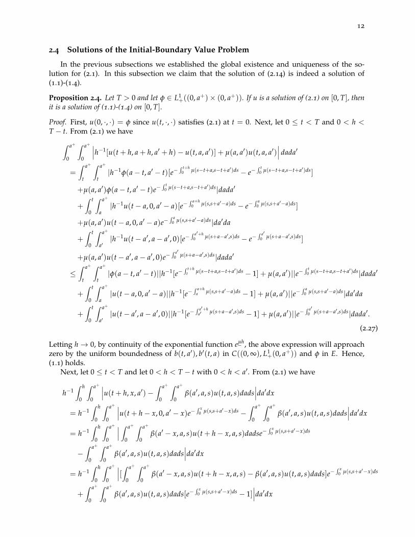
(a) a+ < ∞. (b) a+ = ∞.

Figure 4.1: Integration regions for (4.4) and (A.3).

Moreover, the essential spectral radius of A satisfies that

rEσ(S(t)) = exp[ω1(A)t] ≤ e−µt < 1, t ≥ 0.

It follows that S(t)t≥0 is quasi-compact. The following theorem from Engel and Nagel [18,Theorem 2.5, Chapter VI] will be used to show the stability of an equilibrium for a C0-semigroup.

Theorem 4.5 (Engel and Nagel [18]). Let S(t)t≥0 be a positive strongly continuous semigroup withgenerator A on a Banach lattice LP(Ω, µ), 1 ≤ p < ∞. Then s(A) = ω0, where

s(A) := supReλ : λ ∈ σ(A)

is the spectral bound of A andω0 := lim

t→∞t−1 log(

∥∥S(t)∥∥)

is the growth bound of A.

5 Spectrum Analysis

In order to study the spectral theory, we introduce some definitions and results in positiveoperator theory on ordered Banach spaces from Inaba [24]. For more complete exposition, werefer to Daners and Koch-Medina [8], Heijmans [20], Marek [37], and Sawashima [43].

Let E be a real or complex Banach space and E∗ be its dual (the space of all linear functionalson E). Write the value of f ∈ E∗ at ψ ∈ E as 〈 f , ψ〉. A non-empty closed subset E+ is called acone if the following hold: (1) E+ + E+ ⊂ E+, (2) λE+ ⊂ E+ for λ ≥ 0, (3) E+ ∩ (−E+) = 0.Let us define the order in E such that x ≤ y if and only if y− x ∈ E+ and x < y if and only ify− x ∈ E+ \ 0. The cone E+ is called total if the set ψ− φ : ψ, φ ∈ E+ is dense in E. Thedual cone E∗+ is the subset of E∗ consisting of all positive linear functionals on E; that is, f ∈ E∗+if and only if 〈 f , ψ〉 ≥ 0 for all ψ ∈ E+. ψ ∈ E+ is called a quasi-interior point if 〈 f , ψ〉 > 0 for allf ∈ E∗+ \ 0. f ∈ E∗+ is said to be strictly positive if 〈 f , ψ〉 > 0 for all ψ ∈ E+ \ 0. The cone E+

is called generating if E = E+ − E+ and is called normal if E∗ = E∗+ − E∗+.An ordered Banach space (E,≤) is called a Banach lattice if (1) any two elements x, y ∈ E have

a supremum x ∨ y = supx, y and an infimum x ∧ y = infx, y in E; and (2) |x| ≤ |y| implies‖x‖ ≤ ‖y‖ for x, y ∈ E, where the modulus of x is defined by |x| = x ∨ (−x).

24

Let B(E) be the set of bounded linear operators from E to E. T ∈ B(E) is said to be positiveif T(E+) ⊂ E+. T ∈ B(E) is said to be strongly positive if 〈 f , Tψ〉 > 0 for every pair ψ ∈E+ \ 0, f ∈ E∗+ \ 0. For T, S ∈ B(E), we say T ≥ S if (T − S)(E+) ⊂ E+. A positive operatorT ∈ B(E) is called non-supporting if for every pair ψ ∈ E+ \ 0, f ∈ E∗+ \ 0, there exists apositive integer p = p(ψ, f ) such that 〈 f , Tnψ〉 > 0 for all n ≥ p. The spectral radius and spectralbound of T ∈ B(E) are denoted as r(T) and s(T) respectively. σ(T) denotes the spectrum of Tand σP(T) denotes the point spectrum of T.

From results in Sawashima [43], Marek [37], and Inaba [24], we state the following proposi-tion.

Proposition 5.1. Let E be a Banach lattice and let T ∈ B(E) be compact and non-supporting. Then thefollowing statements hold:

(i) r(T) ∈ σP(T) \ 0 and r(T) is a simple pole of the resolvent, that is r(T) is an algebraicallysimple eigenvalue of T;

(ii) The eigenspace of corresponding to r(T) is one-dimensional and the corresponding eigenvector ψ ∈E+ is a quasi-interior point. The relation Tφ = µφ with φ ∈ E+ implies that φ = cψ for someconstant c;

(iii) The eigenspace of T∗ corresponding to r(T) is also a one-dimensional subspace of E∗ spanned by astrictly positive functional f ∈ E∗+;

(iv) Let S, T ∈ B(E) be compact and non-supporting. Then S ≤ T, S 6= T and r(T) 6= 0 implyr(S) < r(T).

5.1 Point Spectrum and Stability Analysis

In this subsection we study the spectrum of A. Note that we will not solve the characteristicor resolvent equation of A directly, since A with its domain D(A) seems very complicatedas shown in Section 3. But thanks to the solution flow S(t)t≥0, we can still characterize theeigenfunctions or resolvent solutions of A, see the following theorems from Webb [53]. Moreover,we only consider the case a+ < ∞ in this section but the main results presented here remaintrue in the case a+ = ∞ (see Remark 5.8).

Theorem 5.2 (Webb [53]). Let F and G be defined in Proposition 3.1. Then φ ∈ D(A) and Aφ = λφfor some λ ∈ C if and only if φ (in the complexification of E) satisfies

φ(a, a′) =

e−λa′Π(a, a′, a′)F (φ)(a− a′), a.e. a > a′

e−λaΠ(a, a′, a)G(φ)(a′ − a), a.e. a′ > a,(5.1)

whereΠ(a, a′, t) = exp[−

∫ t

0µ(a− τ, a′ − τ)dτ].

Theorem 5.3 (Webb [53]). Let λ ∈ ρ(A) (the resolvent set of A) such that Reλ > βsup + β′sup − µ, letψ ∈ E and satisfy φ = (λI − A)−1ψ. Then

φ(a, a′) =

e−λa′Π(a, a′, a′)F (φ)(a− a′) +∫ a′

0 e−λσΠ(a, a′, σ)ψ(a− σ, a′ − σ)dσ, a.e. a > a′

e−λaΠ(a, a′, a)G(φ)(a′ − a) +∫ a

0 e−λσΠ(a, a′, σ)ψ(a− σ, a′ − σ)dσ, a.e. a′ > a,

(5.2)where βsup + β′sup is from the norm of linear boundary conditions.

25

Plugging (5.1) into the integral conditions F (φ) and G(φ) defined in Proposition 3.1, weobtain

G(φ)(a′) =∫ a+

0

∫ a+

0β(a′, a, s)φ(a, s)dads

=∫ a+

0

∫ a

0β(a′, a, s)Π(a, s, s)e−λsF (φ)(a− s)dsda

+∫ a+

0

∫ s

0β(a′, a, s)Π(a, s, a)e−λaG(φ)(s− a)dads,

F (φ)(a) =∫ a+

0

∫ a+

0β′(a, s, a′)φ(s, a′)dsda′ (5.3)

=∫ a+

0

∫ a′

0β′(a, s, a′)Π(s, a′, s)e−λsG(φ)(a′ − s)dsda′

+∫ a+

0

∫ s

0β′(a, s, a′)Π(s, a′, a′)e−λa′F (φ)(s− a′)da′ds.

Denote

α(t) = G(φ)(t), η(t) = F (φ)(t),f1(a′, a, s) = β(a′, a, s)Π(a, s, s), f2(a′, a, s) = β(a′, a, s)Π(a, s, a),f3(a, s, a′) = β′(a, s, a′)Π(s, a′, s), f4(a, s, a′) = β′(a, s, a′)Π(s, a′, a′).

So

α(t) =∫ a+

0

∫ a

0f1(t, a, s)η(a− s)e−λsdsda +

∫ a+

0

∫ s

0f2(t, a, s)α(s− a)e−λadads,

η(t) =∫ a+

0

∫ a′

0f3(t, s, a′)α(a′ − s)e−λsdsda′ +

∫ a+

0

∫ s

0f4(t, s, a′)η(s− a′)e−λa′da′ds.

(5.4)

If we can solve nontrivial α and η from the above equations, we would find the nontrivialsolution of the characteristic equation. In the following context, the function space appeared isitself or its complexification based on the values of λ in R or C.

Define Fλ : L1(0, a+)× L1(0, a+)→ L1(0, a+)× L1(0, a+), λ ∈ C, by

Fλ(α, η) = (F1λ(α, η), F2λ(α, η)),

where

F1λ(α, η) =∫ a+

0

∫ a


∫ a+

0

∫ s

0f2(t, a, s)α(s− a)e−λadads

and

F2λ(α, η) =∫ a+

0

∫ a′


∫ a+

0

∫ s

0f4(t, s, a′)η(s− a′)e−λa′da′ds.

Now the problem becomes finding a nontrivial fixed point of Fλ in L1(0, a+)× L1(0, a+). Fur-thermore, it is easy to check that Fλ maps L1(0, a+)× L1(0, a+) into itself since

∥∥F1λ(α, η)∥∥ =

∫ a+

0

∫ a+

0

∫ a

0| f1(t, a, s)η(a− s)e−λs|dsdadt +

∫ a+

0

∫ a+

0

∫ s

0| f2(t, a, s)α(s− a)e−λs|dadsdt

≤∫ a+

0β(t)dt

∫ a+

0|η(a− s)|da

∫ a

0e−(Reλ+µ)sds +

∫ a+

0β(t)dt

∫ a+

0|α(s− a)|ds

∫ s

0e−(Reλ+µ)ada

26

≤βsup

Reλ + µ[1− e−(Reλ+µ)a+ ]

∥∥(α, η)∥∥ . (5.5)

Similarly, for F2λ, we also have the following estimate:

∥∥F2λ(α, η)∥∥ ≤ β′sup

Reλ + µ[1− e−(Reλ+µ)a+ ]

∥∥(α, η)∥∥ . (5.6)

In the following we give some properties of Fλ.

Lemma 5.4. Let Assumption 2.1 hold. Then the operator Fλ is compact for all λ ∈ C and non-supportingfor all λ ∈ R.

Proof. For the compactness of Fλ, it is equivalent to show that for a bounded set K of L1(0, a+)×L1(0, a+),

limh→0

∫ a+

0|Fiλ(α, η)(t + h)− Fiλ(α, η)(t)|dt = 0 uniformly for (α, η) ∈ L1(0, a+)× L1(0, a+),

where i = 1, 2. Now let us consider F1λ, that is,∣∣∣ ∫ a+

0

∫ a+

0

∫ a

0f1(t + h, a, s)e−λsη(a− s)dsdadt +

∫ a+

0

∫ a+

0

∫ s

0f2(t + h, a, s)e−λaα(s− a)dadsdt

−∫ a+

0

∫ a+

0

∫ a

0f1(t, a, s)e−λsη(a− s)dsdadt−

∫ a+

0

∫ a+

0

∫ s

0f2(t, a, s)e−λaα(s− a)dadsdt

∣∣∣≤∫ a+

0

∫ a+

0

∫ a

0| f1(t + h, a, s)− f1(t, a, s)||e−λs||η(a− s)|dsdadt

+∫ a+

0

∫ a+

0

∫ s

0| f2(t + h, a, s)− f2(t, a, s)||e−λa||α(s− a)|dadsdt

→ 0 as h→ 0 (5.7)

by Assumption 2.1(ii) on β, β′. Similarly, we can show the convergence for F2λ, which impliesthat Fλ is a compact operator for all λ ∈ C.

Next, for λ ∈ R, define a positive functional Fλ = (F1λ, F2λ) by

〈F1λ, (α, η)〉 :=∫ a+

0

∫ a

0ε1(s)Π(a, s, s)e−λsη(a− s)dsda

+∫ a+

0

∫ s

0ε1(s)Π(a, s, a)e−λaα(s− a)dads,

〈F2λ, (α, η)〉 :=∫ a+

0

∫ a′

0ε2(s)Π(s, a′, s)e−λsα(a′ − s)dsda′

+∫ a+

0

∫ s

0ε2(s)Π(s, a′, a′)e−λaη(s− a′)da′ds. (5.8)

From Assumption 2.1(iii), Fλ is a strictly positive functional and we have

Fλ(α, η) = (F1λ(α, η), F2λ(α, η)) ≥ (〈F1λ, (α, η)〉e1, 〈F2λ, (α, η)〉e2),lim

λ→−∞(〈F1λ, (e1, e2)〉, 〈F2λ, (e1, e2)〉) = (+∞,+∞), (5.9)

where (e1, e2) ≡ 1 is a quasi-interior point in L1(0, a+)× L1(0, a+) when a+ < ∞. Moreover, wehave

F2λ(α, η) = Fλ(F1λ(α, η), F2λ(α, η)) = (F1λ(F1λ(α, η), F2λ(α, η)), F2λ(F1λ(α, η), F2λ(α, η))),

27

where

Fiλ(F1λ(α, η), F2λ(α, η)) ≥ 〈Fiλ, (F1λ(α, η), F2λ(α, η))〉ei

≥ 〈Fiλ,(〈F1λ, (α, η)〉e1, 〈F2λ, (α, η)〉e2

)〉ei

≥ min〈F1λ, (α, η)〉, 〈F2λ, (α, η)〉〈Fiλ, (e1, e2)〉ei

:= min〈Fλ, (α, η)〉〈Fiλ, (e1, e2)〉ei, i = 1, 2.

It follows that

F2λ(α, η) ≥ min〈Fλ, (α, η)〉(〈F1λ, (e1, e2)〉e1, 〈F2λ, (e1, e2)〉e2)

≥ min〈Fλ, (α, η)〉min〈Fλ, (e1, e2)〉(e1, e2).

By induction for any integer n we have

Fn+1λ (α, η) ≥ min〈Fλ, (α, η)〉

[min〈Fλ, (e1, e2)〉

]n(e1, e2).

Then we obtain 〈F , Fnλ (α, η)〉 > 0, n ≥ 1, for every pair (α, η) ∈ L1

+(0, a+)× L1+(0, a+) \ (0, 0), F ∈

(L1+(0, a+))∗ × (L1

+(0, a+))∗ \ (0, 0); that is, we know that Fλ is a non-supporting operator. Insummary, Fλ is a compact and non-supporting operator.

Remark 5.5. Note that in the above proof of non-supporting of Fλ, we chose a constant functione ≡ 1 as the lower bound of Fλ. But if a+ = ∞, e ≡ 1 is no longer in L1(0, ∞) × L1(0, ∞).Fortunately, we can still prove it under Assumption 2.1(iii)’.

Still define the same positive functional Fλ = (F1λ, F2λ) by (5.8). From Assumption 2.1(iii)’,Fλ is a strictly positive functional and we have

Fλ(α, η) = (F1λ(α, η), F2λ(α, η)) ≥ (〈F1λ, (α, η)〉β1, 〈F2λ, (α, η)〉β′1),lim

λ→−∞(〈F1λ, (β1, β′1)〉, 〈F2λ, (β1, β′1)〉) = (+∞,+∞), (5.10)

where (β1, β′1) is obviously a quasi-interior point in L1(0, a+)× L1(0, a+). The estimates are thesame as above by just changing (e1, e2) into (β1, β′1). Hence, Fλ is still a non-supporting operatorwhen a+ = ∞.

Now we study the resolvent set of A. Plugging (5.2) into the integral conditions F (φ) andG(φ) defined in Proposition 3.1, we obtain that

α(t) =∫ a+

0

∫ a


∫ a+

0

∫ s

0f2(t, a, s)α(s− a)e−λadads

+∫ a+

0

∫ a

0K1(t, a, s)ψ(a, s)dsda +

∫ a+

0

∫ s

0K2(t, a, s)ψ(a, s)dads,

η(t) =∫ a+

0

∫ a′


∫ a+

0

∫ s

0f4(t, s, a′)η(s− a′)e−λa′da′ds

+∫ a+

0

∫ a′

0K3(t, s, a′)ψ(s, a′)dsda′ +

∫ a+

0

∫ s

0K4(t, s, a′)ψ(s, a′)da′ds,

(5.11)

whereK1(t, a, s)ψ(a, s) = β(t, a, s)

∫ s

0e−λσΠ(a, s, σ)ψ(a− σ, s− σ)dσ,

K2(t, a, s)ψ(a, s) = β(t, a, s)∫ a

0e−λσΠ(a, s, σ)ψ(a− σ, s− σ)dσ,

K3(t, s, a′)ψ(s, a′) = β′(t, s, a′)∫ s

0e−λσΠ(s, a′, σ)ψ(s− σ, a′ − σ)dσ,

K4(t, s, a′)ψ(s, a′) = β′(t, s, a′)∫ s

0e−λσΠ(s, a′, σ)ψ(s− σ, a′ − σ)dσ.

(5.12)

28

One can rewrite (5.11) as the following functional equations.(αη

)= Fλ

(αη

)+

(G1

λψG2

λψ

), (5.13)

where

G1λψ =

∫ a+

0

∫ a

0K1(t, a, s)ψ(a, s)dsda +

∫ a+

0

∫ s

0K2(t, a, s)ψ(a, s)dads,

G2λψ =

∫ a+

0

∫ a

0K3(t, s, a)ψ(s, a)dsda +

∫ a+

0

∫ s

0K4(t, s, a)ψ(s, a)dads. (5.14)

Next we analyze the spectrum of Fλ and A together with their relations via the continuity ofr(Fλ) with respect to λ and the sign of r(F0)− 1.

Proposition 5.6. Let Assumption 2.1 hold and for a+ < ∞, we have the following statements

(i) Γ := λ ∈ C : 1 ∈ σ(Fλ) = λ ∈ C : 1 ∈ σP(Fλ), where σ(A) and σP(A) denote the spectrumand point spectrum of the operator A, respectively;

(ii) There exists a unique real number λ0 ∈ Γ such that r(Fλ0) = 1 and λ0 > 0 if r(F0) > 1; λ0 = 0 ifr(F0) = 1; and λ0 < 0 if r(F0) < 1;

(iii) λ0 > supReλ : λ ∈ Γ \ λ0;

(iv) λ ∈ C : λ ∈ ρ(A) = λ ∈ C : 1 ∈ ρ(Fλ), where ρ(A) denote the resolvent set of A;

(v) λ0 is the dominant eigenvalue of A, i.e. λ0 is greater than all real parts of the eigenvalues of A.Moreover, it is an algebraically simple eigenvalue of A;

(vi) λ0 = s(A) := supReλ : λ ∈ σ(A).

Proof. (i) Since Fλ is compact, σ(Fλ) \ 0 = σP(Fλ) \ 0, hence conclusion (i) follows.(ii) Next, Fλ, λ ∈ R is strictly decreasing in the operator sense, which implies that the spectral

radius r(Fλ), λ ∈ R, is strictly decreasing by Lemma 5.4 and Proposition 5.1 (see also Inaba [24,Proposition 3.3]). On the one hand, for λ ∈ R, let fλ be a positive eigenfunctional correspondingto the eigenvalue r(Fλ) of positive operator Fλ. Then we have

〈 fλ, Fλ(e1, e2)〉 = r(Fλ)〈 fλ, (e1, e2)〉 ≥ min〈Fλ, (e1, e2)〉〈 fλ, (e1, e2)〉.

Since fλ is strictly positive, we obtain r(Fλ) ≥ min〈Fλ, (e1, e2)〉. It follows from (5.9) thatlim

λ→−∞r(Fλ) = +∞. On the other hand, it is easy to see that lim

λ→∞r(Fλ) = 0. Moreover, by the fact

that the spectral radius of a compact operator is continuous with respect to the parameter fromNussbaum [42] or Degla [9], we conclude the result (ii).

(iii) Next, we can use the idea in Inaba [24, Proposition 3.3] to show result (iii). For anyλ ∈ Γ, there exists an eigenfunction φλ such that Fλφλ = φλ, i.e.(

F1λ(φ1λ, φ2λ)F2λ(φ1λ, φ2λ)

)=

(φ1λ

φ2λ

).

Then we have |φλ| = |Fλφλ| ≤ FReλ|φλ| where |φλ| :=

(|φ1λ||φ2λ|

). Let fReλ be the positive eigen-

functional corresponding to the eigenvalue r(FReλ) of FReλ, we obtain that

〈 fReλ, FReλ|φλ|〉 = r(FReλ)〈 fReλ, |φλ|〉 ≥ 〈 fReλ, |φλ|〉.

29

Hence, we have r(FReλ) ≥ 1 and Reλ ≤ λ0 since r(Fλ) is strictly decreasing with respect toλ ∈ R and r(Fλ0) = 1. If Reλ = λ0, then Fλ0 |φλ| = |φλ|. In fact, if Fλ0 |φλ| > |φλ|, taking dualityparing with the eigenfunctional fλ0 corresponding to the eigenvalue r(Fλ0) = 1 on both sidesyields 〈 fλ0 , Fλ0 |φλ|〉 = 〈 fλ0 , |φλ|〉 > 〈 fλ0 , |φλ|〉, which is a contradiction. Then we can write that|φλ| = cφλ0 , where φλ0 is the eigenfunction corresponding to the eigenvalue r(Fλ0) = 1. Hence,

without loss of generality we can assume that c = 1 and write φλ =

(φ1λ(t)φ2λ(t)

)=

(φ10(t)eiγ(t)

φ20(t)eiζ(t)

)

for some real function γ(t) and ζ(t), where φλ0 =

(φ10(t)φ20(t)

). If we substitute this relation into

Fλ0 φλ0 = φλ0 = |φλ| = |Fλφλ|,

then we have∫ a+

0

∫ a

0f1(t, a, s)φ20(a− s)e−λ0sdsda +

∫ a+

0

∫ s

0f2(t, a, s)φ10(s− a)e−λ0adads

=∣∣∣ ∫ a+

0

∫ a

0f1(t, a, s)φ20(a− s)eiζ(a−s)e−(λ0+iImλ)sdsda

+∫ a+

0

∫ s

0f2(t, a, s)φ10(s− a)eiγ(s−a)e−(λ0+iImλ)adads

∣∣∣and ∫ a+

0

∫ a′

0f3(t, s, a′)φ10(a′ − s)e−λ0sdsda′ +

∫ a+

0

∫ s

0f4(t, s, a′)φ20(s− a′)e−λ0a′da′ds

=∣∣∣ ∫ a+

0

∫ a′

0f3(t, s, a′)φ10(a′ − s)eiγ(a′−s)e−(λ0+iImλ)sdsda′

+∫ a+

0

∫ s

0f4(t, s, a′)φ20(s− a′)eiζ(s−a′)e−(λ0+iImλ)a′da′ds

∣∣∣which follows after changing variables that∫ a+

0

∫ a

0f1(t, a, s)φ20(a− s)e−λ0s + f2(t, s, a)φ10(a− s)e−λ0sdsda

=∣∣∣ ∫ a+

0

∫ a

0f1(t, a, s)φ20(a− s)eiζ(a−s)e−(λ0+iImλ)s + f2(t, s, a)φ10(a− s)eiγ(a−s)e−(λ0+iImλ)sdsda

∣∣∣and∫ a+

0

∫ a′

0f3(t, s, a′)φ10(a′ − s)e−λ0s + f4(t, a′, s)φ20(a′ − s)e−λ0sdsda′

=∣∣∣ ∫ a+

0

∫ a′

0f3(t, s, a′)φ10(a′ − s)eiγ(a′−s)e−(λ0+iImλ)s + f4(t, a′, s)φ20(a′ − s)eiζ(a′−s)e−(λ0+iImλ)sdsda′

∣∣∣From Heijmans [20, Lemma 6.12], we have that ζ(a − s) − Imλs = γ(a − s) − Imλs = θ1 andζ(a′ − s)− Imλs = γ(a′ − s)− Imλs = θ2 for some constants θ1 and θ2. From Fλφλ = φλ, wehave (

eiθ1 F1λ0(φ10, φ20)eiθ2 F2λ0(φ10, φ20)

)=

(eiγφ10eiζφ20

),

which implies that θ1 = γ and θ2 = ζ, hence Imλ = 0. Then there is no element λ ∈ Γ such thatReλ = λ0 and λ 6= λ0, thus result (iii) is desired.

30

(iv) For result (iv), when 1 ∈ ρ(Fλ), (I − Fλ)−1 exists and is well-defined, then from (5.13),

one can obtain that (αη

)= (I − Fλ)

−1

(G1

λψG2

λψ

)(5.15)

Now plugging (5.15) into (5.2), we will obtain the expression of ϕ = (λI − A)−1ψ, which iswell-defined. It follows that λ ∈ ρ(A). Conversely, if λ ∈ ρ(A), the resolvent solution (5.2) existsand is well-defined, then the integral equations (5.11) on (α, η) has a solution. It follows that(5.13) has a solution, which implies that 1 ∈ ρ(Fλ).

(v) First claim that λ ∈ σP(A) with geometric multiplicity m if and only if 1 ∈ σP(Fλ)with geometric multiplicity m for all m ∈ N. In fact, if λ ∈ σP(A) corresponding to lin-early independent eigenfunctions φ1, ..., φm, then φ1, ..., φm satisfy (5.1) which implies that (5.3)holds and equivalently (5.4) holds. It follows that Fλ(G(φi),F (φi)) = (G(φi),F (φi)) for alli = 1, ..., m. Hence (G(φi),F (φi)), i = 1, ..., m, are necessarily linearly independent eigenfunc-tions of Fλ corresponding to eigenvalue 1 and so 1 ∈ σP(Fλ) with geometric multiplicity n ≥ m.Conversely, if (αi, ηi), i = 1, ..., n, are eigenfunctions of Fλ corresponding to eigenvalue 1, i.e.Fλ(αi, ηi) = (αi, ηi), i = 1, ..., n, and set

φi(a, a′) =

e−λa′Π(a, a′, a′)ηi(a− a′), a′ < a,e−λaΠ(a, a′, a)αi(a′ − a), a < a′,

i = 1, ..., n. (5.16)

Then it is easy to verify F (φi) = ηi,G(φi) = αi, i = 1, ..., n. It follows that λφi = Aφi, i = 1, ..., n,by Theorem 5.2. Moreover, (5.16) ensures that φ1, ..., φn are linearly independent. Hence, λ ∈σP(A) with at geometric multiplicity m ≥ n. Thus n = m. It follows from the claim that

Γ = λ ∈ C : λ ∈ σP(A).

Now from (iii), we conclude that λ0 is dominant. Next, we need to prove that λ0 is simple.Plugging (5.15) into (5.2), we obtain

(λI − A)−1ψ =

e−λa′Π(a, a′, a′)(I − Fλ)

−11 (G1

λψ, G2λψ)(a− a′)

+∫ a′

0 e−λσΠ(a, a′, σ)ψ(a− σ, a′ − σ)dσ a.e. a > a′

e−λaΠ(a, a′, a)(I − Fλ)−12 (G1

λψ, G2λψ)(a′ − a)

+∫ a

0 e−λσΠ(a, a′, σ)ψ(a− σ, a′ − σ)dσ a.e. a′ > a,

where (I − Fλ)−1 = ((I − Fλ)

−11 , (I − Fλ)

−12 ). From the above formula, we see that (λI − A)−1

does not hold for all λ such that r(Fλ) = 1. Thus, 1 is a pole of (I − Fλ)−1 of order m if and

only if λ is a pole of (λI − A)−1 of order m. However, by Proposition 5.1 (i), we know that 1 is asimple pole of (I − Fλ)

−1 which implies that λ0 is a simple pole of (λI − A)−1. Thus it followsfrom Webb [52, Proposition 4.11] that λ0 is an algebraically simple eigenvalue of A.

(vi) Finally, we show result (vi). Let λ0 := s(A) denote the spectral bound of A. Then λ0 ≥ λ0and so λ0 > ω1(A) = −∞. Thus σ0(A) = λ0 by Webb [54, Proposition 2.5] which states thatthe peripheral spectrum σ0 of the generator of a strongly continuous positive semigroup in aBanach lattice consists exactly of the generator’s spectral bound provided the latter is strictlygreater than the essential growth bound. Then λ0 ∈ σ(A) and thus by (i) and (iv), 1 ∈ σp(Fλ0

),which implies that 1 ≤ r(Fλ0

). However, due to λ0 ≥ λ0 we have r(Fλ0) ≤ r(Fλ0) = 1, Hence,

λ0 = λ0. Thus (vi) is desired.

To address the case when a+ = ∞, we make the following assumption.

31

Assumption 5.7. r(Fγ) > 1 for some γ ∈ R with γ > −µ.

Remark 5.8. For a+ = ∞, if in addition we have Assumption 5.7, all statements in Proposition5.6 still hold.

It guarantees the existence of λ0 such that r(Fλ0) = 1 since for now the domain of Fλ ischanging into Reλ > −µ instead of C to make Fλ be well-defined. Further, for Proposition5.6(vi) one can see that λ0 ≥ λ0 > γ > −µ ≥ ω1(A) when a+ = ∞. Note the Assumption5.7 is only used here to show the existence of λ0 under the case a+ = ∞. All other resultsin this Section 5 are still valid without this assumption. Moreover, the Assumption 5.7 can beverified explicitly given the separable mixing Assumption 2.1(iii’) plus β2 ≡ β′2. In fact, it’seasy to compute F0(β1, β′1) = r(F0)(β1, β′1) under the condition and then r(F0) > 1 will impliesAssumption 5.7, where

r(F0) =∫ a+

0

∫ a

0β2(a, s)Π(a, s, s)β′1(a− s)dsda +

∫ a+

0

∫ s

0β2(a, s)Π(a, s, a)β1(s− a)dads.

Remark 5.9. In fact, we can prove (vi) by using a different method. Observe that for any λ ∈ R,when λ > λ0 and so r(Fλ) < r(Fλ0) = 1, (I− Fλ)

−1 exists and is positive. Moreover, 1 ∈ ρ(Fλ)⇒λ ∈ ρ(A). Therefore, λ0 is larger than any other real spectral values in σ(A). It follows thatλ0 = sR(A) := supλ ∈ R : λ ∈ σ(A). Next we claim A is a resolvent positive operator. Infact, it is easy to see that the resolvent set of A contains an infinite ray (λ0, ∞) and (λI − A)−1

is a positive operator for λ > λ0 by (5.2) and the positivity of (I − Fλ)−1. But since L1(0, a+)×

L1(0, a+) is a Banach lattice with normal and generating cone K := L1+(0, a+)× L1

+(0, a+) ands(A) ≥ λ0 > −∞ due to λ0 ∈ σ(A), we can conclude from Thieme [47, Theorem 3.5] thats(A) = sR(A) = λ0.

Remark 5.10. As we know, non-supporting is a generalization of strong positivity in the Banachspace with a positive cone which may have empty interior. In fact, we can give an assumption onβ and β′ such that Fλ is strongly positive in the sense of dual space (see the definition in Danersand Koch-Medina [8]), for example Assumption 2.1(iii)’. Now Fλ itself is strongly positive thusirreducible in L1(0, a+)× L1(0, a+) which is a Banach lattice, then by [8, Theorem 12.3], one canstill conclude that r(Fλ) is an algebraically simple eigenvalue of Fλ with a positive eigenfunctionand a simple pole of the resolvent of Fλ. Moreover, λ→ r(Fλ) is continuous by the compactnessof Fλ and strictly decreasing by showing that λ → r(Fλ) is log-convex Thieme [47] or super-convex Kato [30], for details see [2, Lemma 1]. Hence, we can still obtain the same results inProposition 5.6.

Taking a closer look at the operator F0, we have its first output element illustrated as:

F10(α, η)(b) =∫ a+

0

∫ a

0β(b, a, s)Π(a, s, s)η(a− s)dsda︸︷︷︸

next generation population density with structure (0,b)produced by first generation with structure (·,0)

and density function η(·)

+∫ a+

0

∫ s

0β(b, a, s)Π(a, s, a)α(s− a)dads︸︷︷︸

next generation population density with structure (0,b)produced by first generation with structure (0,·)

and density function α(·)

,

where η(a− s) is the first generation population density with structure (a− s, 0), Π(a, s, s) is thesurvival probability for individuals born with structure (a− s, 0) to reach structure (a, s), andβ(b, a, s) is the reproduction rate for mothers with structure (a, s) to give birth to daughters withstructure (0, a). And the interpretation of the second integral follows similarly.

Biologically speaking, F0 is the next generation operator: given any population density func-tions (α(·), η(·)) on both boundaries (first generation densities), F0(α(·), η(·)) represents the

32

offspring density functions (second generation) on both boundaries generated by the first gen-eration during their entire life periods. Thus the spectral radius of F0 can be interpreted as thebasic reproductive number of the population, where a detailed mathematical interpretation canbe adopted directly from the widely known discussion on R0 for single-structured infectiousdisease models (Diekmann et al. [12]) or scalar age-structured population dynamical models(Kot [32]). Therefore, we have the following theorem by Theorem 4.5 on the basic reproductionnumber R0.

Theorem 5.11. Define R0 := r(F0). If R0 < 1, then the zero equilibrium is globally exponentiallystable. Otherwise, if R0 > 1, then the zero equilibrium is unstable.

Proof. If R0 = r(F0) < 1, by Proposition 5.6(ii) there exists a unique real λ0 < 0 such thatr(Fλ0) = 1. Hence by Proposition 5.1 we have Fλ0 ϕλ0 = r(Fλ0)ϕλ0 = ϕλ0 which ϕλ0 is a positivefunction in L1(0, a+)× L1(0, a+); that is, we find a nontrivial solution ϕλ0 of the characteristicequations for some λ < 0 when r(F0) < 1. Moreover, there is no nontrivial solution for all λ > 0since 0 is the only fixed point of Fλ by Banach Fixed Point Theorem. And from Proposition5.6(iv) we know that s(A) := supReλ : λ ∈ σ(A) = λ0 < 0. It follows from Theorem 4.5 thatthe zero equilibrium is globally exponentially stable.

If R0 = r(F0) > 1, by Proposition 5.6(v) there exists a real λ0 > 0 such that r(Fλ0) = 1. Sim-ilarly, by Proposition 5.1 we have Fλ0 ϕλ0 = r(Fλ0)ϕλ0 = ϕλ0 , in which ϕλ0 is a positive functionin L1(0, a+)× L1(0, a+); that is, we find a nontrivial solution ϕλ0 of the characteristic equationfor some λ > 0 when r(F0) > 1. Moreover, by Proposition 5.6(vi), s(A) = λ0 > 0. Motivatedby Thieme [46, Corollary 4.3], let Σ denote the set of spectral values with positive real parts. Asthese are normal eigenvalues, Σ is finite and bounded away from the imaginary axis and can sobe separated from the rest of the spectrum by a rectifiable simple closed curve. According toKato [31, Chapter III, Theorem 6.17], there exists a decomposition of E into invariant subspacesE1 and E2 such that the restriction of A to E1 has the spectrum Σ and its restriction to E2 has aspectral bound ≤ 0 < infReλ : λ ∈ Σ and thus a non-positive type. Now the instability of thezero equilibrium follows from Desch and Schappacher [11, Theorem 2.2].

Furthermore, it is easy to check that Fλ maps L1(0, a+)× L1(0, a+) into itself since∥∥F1λ(α, η)∥∥ =

∫ a+

0

∫ a+

0

∫ a

0| f1(t, a, s)η(a− s)e−λs|dsdadt

+∫ a+

0

∫ a+

0

∫ s

0| f2(t, a, s)α(s− a)e−λs|dadsdt

≤∫ a+

0β(t)dt

∫ a+

0|η(a− s)|da

∫ a

0e−(Reλ+µ)sds

+∫ a+

0β(t)dt

∫ a+

0|α(s− a)|ds

∫ s

0e−(Reλ+µ)ada

≤βsup

Reλ + µ

∥∥(α, η)∥∥ . (5.17)

Similarly, for F2λ, we also have the following estimate:∥∥F2λ(α, η)∥∥ ≤ β′sup

Reλ + µ

∥∥(α, η)∥∥ . (5.18)

Remark 5.12. In general r(F0) is not easy to compute, but we have the following estimatescombining (5.5), (5.6), (5.17) and (5.18) when a+ < ∞:

‖Fλ‖ ≤βmax

Reλ + µ[1− e−(Reλ+µ)a+ ], (5.19)

33

and when a+ = ∞,

‖Fλ‖ ≤βmax

Reλ + µ. (5.20)

Then by the Gelfand’s formula r(F) = limk→∞

∥∥∥Fk∥∥∥ 1

k for bounded linear operators and linearity of

Fλ, we have

r(F0) ≤

βmax(1−e−µa+)

µ , when a+ < ∞,βmax

µ , when a+ = ∞.

Thus, we have the following corollary.

Corollary 5.13. (i) When a+ < ∞, if βmax(1−e−µa+ )µ < 1, then the zero equilibrium is globally exponen-

tially stable;(ii) When a+ = ∞, if βmax

µ < 1, then the zero equilibrium is globally exponentially stable.

5.2 Asynchronous Exponential Growth

In this subsection, we study the asynchronous exponential growth of S(t)t≥0 when r(F0) >1. We study the two cases when a+ < ∞ and when a+ = ∞ together and give an extra Assump-tion 5.7 in the latter case. First let us recall the definition.

Definition 5.14. Let S(t)t≥0 be a strongly continuous semigroups of bounded linear operatorson a Banach space X with infinitesimal generator A. We say that S(t)t≥0 has asynchronousexponential growth with intrinsic growth constant λ0 ∈ R if there exists a nonzero finite rankoperator P0 ∈ X such that

limt→∞

e−λ0tS(t) = P0.

We introduce a theorem in Magal and Ruan [35, Theorem 4.6.2] which was proved by Webb[54].

Theorem 5.15 (Webb [54]). Let S(t)t≥0 be a strongly continuous semigroup of bounded linear opera-tors on a Banach space X with infinitesimal generator A. Then S(t)t≥0 has asynchronous exponentialgrowth with intrinsic growth constant λ0 ∈ R if and only if

(i) ω1(A) < λ0;

(ii) λ0 = supReλ : λ ∈ σ(A);

(iii) λ0 is a simple pole of (λI − A)−1.

where ω1(A) denotes the essential growth bound of A which is defined by (4.9).

Now we use this theorem to show that our semigroup S(t)t≥0 defined in (2.14) has asyn-chronous exponential growth.

Theorem 5.16. If R0 > 1, then there exists a unique positive and real number λ1 > −µ satisfyingr(Fλ1) = 1 such that S(t)t≥0 has asynchronous exponential growth with intrinsic growth constant λ1.Moreover,

limt→∞

e−λ1tS(t)φ = Pλ1 φ for all φ ∈ E,

34

where Pλ1 : E→ E is defined by

Pλ1 φ = (2πi)−1∫

Γ(λI − A)−1φdλ

and Γ is a positively oriented closed curve in C enclosing λ1, but no other point of σ(A).

Proof. First it is easy to see that if r(F0) > 1, then there exists a unique real number λ1 > 0 suchthat r(Fλ1) = 1 and λ1 = supReλ : λ ∈ σ(A) by Proposition 5.6, which shows that condition(ii) in Theorem 5.15 holds. Next, in Section 4 we have shown that ω1(A) ≤ −µ for a+ = ∞and ω1(A) = −∞ when a+ < ∞. Thus, condition (i) in Theorem 5.15 is satisfied. Moreover,supReλ : λ ∈ σe(A) ≤ ω1(A), which implies λ1 ∈ σP(A) \ σe(A), thus is a pole of (λI − A)−1

by Webb [52, Proposition 4.11], where σe(A) represents the essential spectrum of A. Also λ1 isa simple eigenvalue of A and a simple pole of (λI − A)−1, see the proof in Proposition 5.6(v).Thus, condition (iii) in Theorem 5.15 is also satisfied. Hence, our result is desired.

What we do next is to derive a formula for the projection Pλ1 : E→ ker(A− λ1 I), inspired byWalker [49]. Observe that there is a quasi-interior element Φ0 = (α, η) ∈ L1

+(0, a+)× L1+(0, a+)

such that ker(1− Fλ1) =spanΦ0. Denote

Πλ(a, a′)(α, η) =

e−λa′Π(a, a′, a′)η(a− a′), a > a′

e−λaΠ(a, a′, a)α(a′ − a), a < a,

then ker(A − λ1 I) =spanΠλ1(a, a′)Φ0. Let φ ∈ E be fixed and let c(φ) ∈ R be such thatPλ1 φ = c(φ)Πλ1(a, a′)Φ0. Recall that λ1 is a simple pole of the resolvent (λI − A)−1. Denote

Hλφ :=

∫ a′

0 e−λσΠ(a, a′, σ)φ(a− σ, a′ − σ)dσ, a′ < a,∫ a0 e−λσΠ(a, a′, σ)φ(a− σ, a′ − σ)dσ, a < a′.

Then Hλφ is holomorphic in λ, it follows that from (5.2), (5.15) and Residue theorem that

Pλ1 φ = limλ→λ1

(λ− λ1)Πλ(a, a′)(1− Fλ)−1Gλφ,

whereGλφ =

(G1

λφ, G2λφ)

,

in which Giλ, i = 1, 2, is defined in (5.14). Let w′ ∈ (L1

+(0, a+)× L1+(0, a′))′ be a positive eigen-

functional of the dual operator F′λ1of Fλ1 corresponding to the eigenvalue r(Fλ1) = 1. Then for

f ′ ∈ E′ defined by〈 f ′, ψ〉 := 〈w′, (Gψ,Fψ)〉, ψ ∈ E,

we have due to F′λ1w′ = w′ that

c(φ)〈w′, Φ0〉 = 〈 f ′, Pλ1 φ〉 = limλ→λ1〈 f ′, (λ− λ1)Πλ(a, a′)(1− Fλ)

−1Gλφ〉

= limλ→λ1〈w′, (λ− λ1)(1− (1− Fλ))(1− Fλ)

−1Gλφ〉

= limλ→λ1〈w′, (λ− λ1)(1− Fλ)

−1Gλφ〉.

WritingGλφ = d(Gλφ)Φ0 ⊕ (1− Fλ1)g(Gλφ) (5.21)

35

according to the decomposition L1+(0, a+)× L1

+(0, a+) = R ·Φ0 ⊕ rg(1− Fλ1), it follows that

limλ→λ1〈w′, (λ− λ1)(1− Fλ)

−1Gλφ〉 = d(Gλ1 φ) limλ→λ1〈w′, (λ− λ1)(1− Fλ)

−1Φ0〉

due to the continuity of Fλ in λ. But from (5.21)

〈w′, Gλ1 φ〉 = d(Gλ1 φ)〈w′, Φ0〉

since F′λ1w′ = w′, whence d(Gλ1 φ) = ξ〈w′, Gλ1 φ〉 with ξ−1 = 〈w′, Φ0〉. Similarly, decomposing

Zλ := (λ− λ1)(1− Fλ)−1Φ0,

we find

limλ→λ1〈w′, Zλ〉 =

(lim

λ→λ1d(Zλ)

)〈w′, Φ0〉.

With these observations, we derive that

c(φ)〈w′, Φ0〉 = C0〈w′, Gλ1 φ〉〈w′, Φ0〉

for some constant C0. Consequently,

Pλ1 φ = C0〈w′, Gλ1 φ〉Πλ1(a, a′)Φ0.

Since Pλ1 is a projection, i.e. P2λ1

= Pλ1 , the constant C0 is easily computed and we obtain thefollowing result.

Proposition 5.17. Under the assumptions of Theorem 5.16, the projection Pλ1 is given by

Pλ1 φ =〈w′, Gλ1 φ〉

〈w′, Gλ1 Πλ1(a, a′)Φ0〉Πλ1(a, a′)Φ0 (5.22)

for φ ∈ E, where Gλ1 φ = (G1λ1

φ, G2λ1

φ) and w′ ∈ (L1+(0, a+)× L1

+(0, a′))′ is a positive eigenfunctionalof the dual operator F′λ1

of Fλ1 corresponding to the eigenvalue r(Fλ1) = 1.

Remark 5.18. In fact, the expression of Pλ1 φ does not look explicitly like the one for singleage-structured models, since the resolvent of A cannot be expressed explicitly for our doubleage-structure model.

5.3 Asymptotic Behavior for R0 = 1

In the previous subsections, we have shown that if R0 < 1, then S(t)t≥0 is uniformlyexponentially stable and if R0 > 1, then S(t)t≥0 has asynchronous exponential growth. It isnatural to ask what happens if R0 = 1.

Remark 5.19. When S(t)t≥0 has asynchronous exponential growth with intrinsic growth con-stant λ1, the intrinsic growth constant λ1 can be any real number, it means that

(i) If λ1 < 0, then S(t) decays exponentially, thus the zero equilibrium is exponentially stable,as Theorem 5.11 states;

(ii) If λ1 > 0, as S(t)t≥0 has asynchronous exponential growth, it describes the divergent rateat which the system blows up when the zero equilibrium is unstable for a linear system;

36

(iii) If λ1 = 0, then S(t)φ converges to Pφ as t → ∞. This is the case when R0 = 1 that we areconcerned in this subsection.

First, note that when R0 = 1, i.e. r(F0) = 1, by the previous argument we know that thespectral bound s(A) = 0. Now let us recall a theorem from Engel and Nagel [18, Chapter VI,Theorem 3.5].

Theorem 5.20 (Engel and Nagel [18]). Let S(t)t≥0 be a quasi-compact, irreducible, positive stronglycontinuous semigroup with generator A and assume that s(A) = 0. Then 0 is a dominant eigenvalue ofA and a first-order pole of (λI − A)−1. Moreover, there exist strictly positive elements 0 h ∈ X, 0ϕ ∈ X′ and constants M ≥ 1, ε > 0 such that∥∥S(t) f − 〈 f , ϕ〉 · h

∥∥ ≤ Me−εt∥∥ f∥∥ for all t ≥ 0, f ∈ X,

where 〈·, ·〉 is the dual product in Banach space.

In section 4, we have shown that S(t)t≥0 is quasi-compact when a+ = ∞; in section 2, wehave shown that S(t)t≥0 is positive. Next, we claim that S(t)t≥0 is also irreducible. Recallthat a positive semigroup with generator A on the Banach lattice X is irreducible if for someλ > s(A) and all 0 < f ∈ X, the resolvent satisfies (λI − A)−1 f 0, where representsstrictly positivity.

By strict positivity in E, we need to require that ϕ = (λI − A)−1ψ > 0 for almost all (a, a′) ∈(0, a+)× (0, a+) for every 0 < ψ ∈ E. Look at the resolvent solution (5.2), we only need that α andη are positive almost everywhere for (a, a′) ∈ (0, a+)× (0, a+). Since α and η are determined by(5.11), motivated by Engel and Nagel [18, Theorem 4.4], only for β and β′, there exists no a0 ≥ 0such that

β∣∣∣[a0,a+)×[a0,a+)×[a0,a+)

= 0, β′∣∣∣[a0,a+)×[a0,a+)×[a0,a+)

= 0 almost everywhere. (5.23)

In fact, Assumption 2.1(iii)’ satisfies the above conditions, then α and η will be positive almosteverywhere. Thus, (λI − A)−1ψ 0, which implies that S(t)t≥0 is irreducible. By Theorem5.20, we have the following theorem.

Theorem 5.21. If R0 = 1 and (5.23) holds, then there exist a strictly positive linear function h ∈ E, alinear form ζ ∈ fix(S(t)′), t ≥ 0, and constants M ≥ 1, ε > 0 such that∥∥S(t)φ− 〈φ, ζ〉 · h

∥∥ ≤ Me−εt∥∥φ∥∥ for all t ≥ 0, φ ∈ E,

wherefix(S(t))t≥0 := x ∈ E : S(t)x = x for all t ≥ 0,

which coincides with ker A and fix(S(t)′)t≥0 = ker(A′).

6 Discussion

In this paper we considered a linear first-order hyperbolic partial differential equation thatmodels the single-species population dynamics with two physiological structures. By usingsemigroup theory, we studied the basic properties and dynamics of the model, including thesolution flow u(t, a, a′) and its semigroup S(t)t≥0 with infinitesimal generator A. Moreover,we established the compactness of the solution trajectories, analyzed the spectrum of A, andinvestigated stability of the zero equilibrium with asynchronous exponential growth.

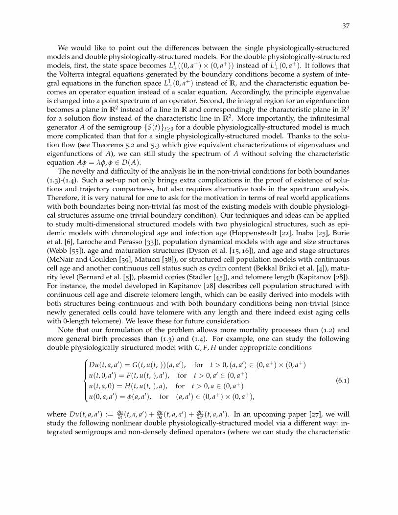
37

We would like to point out the differences between the single physiologically-structuredmodels and double physiologically-structured models. For the double physiologically-structuredmodels, first, the state space becomes L1

+((0, a+)× (0, a+)) instead of L1+(0, a+). It follows that

the Volterra integral equations generated by the boundary conditions become a system of inte-gral equations in the function space L1

+(0, a+) instead of R, and the characteristic equation be-comes an operator equation instead of a scalar equation. Accordingly, the principle eigenvalueis changed into a point spectrum of an operator. Second, the integral region for an eigenfunctionbecomes a plane in R2 instead of a line in R and correspondingly the characteristic plane in R3

for a solution flow instead of the characteristic line in R2. More importantly, the infinitesimalgenerator A of the semigroup S(t)t≥0 for a double physiologically-structured model is muchmore complicated than that for a single physiologically-structured model. Thanks to the solu-tion flow (see Theorems 5.2 and 5.3 which give equivalent characterizations of eigenvalues andeigenfunctions of A), we can still study the spectrum of A without solving the characteristicequation Aφ = λφ, φ ∈ D(A).

The novelty and difficulty of the analysis lie in the non-trivial conditions for both boundaries(1.3)-(1.4). Such a set-up not only brings extra complications in the proof of existence of solu-tions and trajectory compactness, but also requires alternative tools in the spectrum analysis.Therefore, it is very natural for one to ask for the motivation in terms of real world applicationswith both boundaries being non-trivial (as most of the existing models with double physiologi-cal structures assume one trivial boundary condition). Our techniques and ideas can be appliedto study multi-dimensional structured models with two physiological structures, such as epi-demic models with chronological age and infection age (Hoppensteadt [22], Inaba [25], Burieet al. [6], Laroche and Perasso [33]), population dynamical models with age and size structures(Webb [55]), age and maturation structures (Dyson et al. [15, 16]), and age and stage structures(McNair and Goulden [39], Matucci [38]), or structured cell population models with continuouscell age and another continuous cell status such as cyclin content (Bekkal Brikci et al. [4]), matu-rity level (Bernard et al. [5]), plasmid copies (Stadler [45]), and telomere length (Kapitanov [28]).For instance, the model developed in Kapitanov [28] describes cell population structured withcontinuous cell age and discrete telomere length, which can be easily derived into models withboth structures being continuous and with both boundary conditions being non-trivial (sincenewly generated cells could have telomere with any length and there indeed exist aging cellswith 0-length telomere). We leave these for future consideration.

Note that our formulation of the problem allows more mortality processes than (1.2) andmore general birth processes than (1.3) and (1.4). For example, one can study the followingdouble physiologically-structured model with G, F, H under appropriate conditions

Du(t, a, a′) = G(t, u(t, ))(a, a′), for t > 0, (a, a′) ∈ (0, a+)× (0, a+)u(t, 0, a′) = F(t, u(t, ), a′), for t > 0, a′ ∈ (0, a+)u(t, a, 0) = H(t, u(t, ), a), for t > 0, a ∈ (0, a+)u(0, a, a′) = φ(a, a′), for (a, a′) ∈ (0, a+)× (0, a+),

(6.1)

where Du(t, a, a′) := ∂u∂t (t, a, a′) + ∂u

∂a (t, a, a′) + ∂u∂a′ (t, a, a′). In an upcoming paper [27], we will

study the following nonlinear double physiologically-structured model via a different way: in-tegrated semigroups and non-densely defined operators (where we can study the characteristic

38

and resolvent equations directly),

Du(t, a, a′) = −µ(a, a′, P(t))u(t, a, a′), for t > 0, (a, a′) ∈ (0, a+)× (0, a+)

u(t, 0, a′) =∫ a+

0

∫ a+

0 β(a′, a, s, P(t))u(t, a, s)dads, for t > 0, a′ ∈ (0, a+)

u(t, a, 0) =∫ a+

0

∫ a+

0 β′(a, s, a′, P(t))u(t, s, a′)dsda′, for t > 0, a ∈ (0, a+)u(0, a, a′) = φ(a, a′), for (a, a′) ∈ (0, a+)× (0, a+)

P(t) =∫ a+

0

∫ a+

0 u(t, a, a′)dada′, for t > 0.

(6.2)

A Appendix

In this Appendix, we prove some statements that were used in section 4.

Proposition A.1. If a+ = ∞, µ > 0, and Assumption 2.1 holds, then S1(t) satisfies the hypothesis (ii)and S2(t), S3(t) satisfy the hypothesis (iii) of Proposition 4.2.

Proof. We only need to show that S2(t) is compact for t > 0, which is equivalent to show thatfor a bounded set K of E,

limh→0k→0

∫ ∞

0

∫ ∞

0

∣∣∣S2(t)φ(a + h, a′ + k)− S2(t)φ(a, a′)∣∣∣dada′ = 0 (A.1)

and

limh→∞k→∞

∫ ∞

h

∫ ∞

k

∣∣∣S2(t)φ(a, a′)∣∣∣dada′ = 0 (A.2)

uniformly for φ ∈ K (which can be found in [14, Theorem 21, p. 301]). Without loss of generality,assume k > h and h, k→ 0+, we have∫ ∞

0

∫ ∞

0


≤∫ t−h

0

∫ ∞

a

∣∣∣S2(t)φ(a + h, a′ + k)− S2(t)φ(a, a′)∣∣∣da′da︸︷︷︸

region I

+∫ t−h

k−h

∫ a

a+h−k

∣∣∣S2(t)φ(a + h, a′ + k)∣∣∣da′da︸︷︷︸

region II

+∫ k−h

0

∫ a

0

∣∣∣S2(t)φ(a + h, a′ + k)∣∣∣da′da︸︷︷︸

region III

+∫ t

t−h

∫ ∞

a

∣∣∣S2(t)φ(a, a′)∣∣∣da′da︸︷︷︸

region IV

, (A.3)

as illustrated in Figure 4.1b: S2(t)φ(a, a′) is non-trivial for points (a, a′) in regions I and IV, andS2(t)φ(a + h, a′ + k) is non-trivial for points (a, a′) in regions I, II, and III.

We first show∫ t−h

0

∫ ∞

a


≤∫ t

0

∫ ∞

a

∣∣∣bφ(t− a− h, a′ + k− a− h)− bφ(t− a, a′ − a)∣∣∣e− ∫ a+h

0 µ(s,s+a′+k−a−h)dsda′da

+∫ t−h

0

∫ ∞

a

∣∣∣bφ(t− a, a′ − a)[e−∫ a+h

0 µ(s,s+a′+k−a−h)ds − e−∫ a

0 µ(s,s+a′−a)ds]∣∣∣da′da

:= I + II,

39

where

II ≤∫ t−h

0

∫ ∞


∣∣∣e− ∫ a+h0 µ(s,s+a′−a)ds[1− e

∫ a+h0 µ(s,s+a′−a)−µ(s,s+a′+k−a−h)ds]

+ e−∫ a

0 µ(s,s+a′−a)ds[1− e−∫ a+h

a µ(s,s+a′−a)ds]∣∣∣da′da

≤∫ t−h

0

∫ ∞


(max1− e−Kµ(k−h)t, eKµ(k−h)t − 1+ (1− e−µh)

)da′da

≤(

max1− e−Kµ(k−h)t, eKµ(k−h)t − 1+ (1− e−µh)) ∫ t

0

∫ ∞

0bφ(t− a, s)dsda

≤2βmax∥∥φ∥∥

E

(max1− e−Kµ(k−h)t, eKµ(k−h)t − 1+ (1− e−µh)

) ∫ t

0e4βmax(t−a)da

based on our prior estimate in section 2.1 and with Kµ being the Lipschitz constant for µ, thusII→ 0 uniformly for φ ∈ K as h, k→ 0+. Next, we need to show that

limh→0k→0

∫ t

0

∫ ∞

a|bφ(t− a− h, a′ + k− a− h)− bφ(t− a, a′ − a)|da′da = 0 (A.4)

Now by an alternative version of (2.7) and (2.8), we have∫ t

0

∫ ∞

a|bφ(t− a− h, a′ + k− a− h)− bφ(t− a, a′ − a)|da′da

≤∫ t

0

∫ ∞

a

∣∣∣ ∫ t−a−h

0

∫ ∞


−∫ t−a

0

∫ ∞


∣∣∣da′da

+∫ t

0

∫ ∞

a

∣∣∣ ∫ t−a−h

0

∫ ∞

0g1(a′ + k− a− h, p + t− a− h− s, t− a− h− s)b′φ(s, p)dpds

−∫ t−a

0

∫ ∞

0g1(a′ − a, p + t− a− s, t− a− s)b′φ(s, p)dpds

∣∣∣da′da

+∫ t

0

∫ ∞

a

∣∣∣ ∫ ∞

0

∫ ∞

0h1(a′ + k− a− h, p, s, t− a− h)φ(p, s)dpds

−∫ ∞

0

∫ ∞

0h1(a′ − a, p, s, t− a)φ(p, s)dpds

∣∣∣da′da

:= J1 + J2 + J3,

where

J1 ≤∫ t

0

∫ ∞

a

( ∫ t−a−h

0

∫ ∞

0| f1(a′ + k− a− h, t− a− h− p, s + t− a− h− p)

− f1(a′ − a, t− a− p, s + t− a− p)|bφ(p, s)dsdp

+∫ t−a−h

t−a

∫ ∞


)da′da

:=J11 + J2

1,

in which

| f1(a′ + k− a− h, t− a− h− p, s + t− a− h− p)− f1(a′ − a, t− a− p, s + t− a− p)|

≤ β1(a′ + k− a− h)∣∣∣β2(t− a− h− p, s + t− a− h− p)e−

∫ t−a−p−h0 µ(σ,σ+s)dσ

40

− β2(t− a− p, s + t− a− p)e−∫ t−a−p

0 µ(σ,σ+s)dσ∣∣∣

+ |β1(a′ + k− a− h)− β1(a′ − a)|β2(t− a− p, s + t− a− p)

≤ β1(a′ + k− a− h)∣∣∣β2(t− a− h− p, s + t− a− h− p)− β2(t− a− p, s + t− a− p)

∣∣∣+ β1(a′ + k− a− h)β2(t− a− p, s + t− a− p)

∣∣∣1− e−∫ t−a−p

t−a−h−p µ(σ,σ+s)dσ∣∣∣

+∣∣∣β1(a′ + k− a− h)− β1(a′ − a)

∣∣∣β2(t− a− p, s + t− a− p)

≤ β1(a′ + k− a− h)Kβ2h + β(a′ + k− a− h)(1− eµh)

+∣∣∣β1(a′ + k− a− h)− β1(a′ − a)

∣∣∣β2(t− a− p, s + t− a− p)

≤ β1(a′ + k− a− h)Kβ2h + β(a′ + k− a− h)(1− eµh)

+∣∣∣β1(a′ + k− a− h)− β1(a′ − a)

∣∣∣βsup2

by Assumption 2.1(i) on β being Lipschitz continuous and Kβ as the Lipschitz constant, where

βsup2 := sup

(a,s)∈(0,∞)×(0,∞)

β2(a, s) < ∞

because Assumption 2.1(iv) holds. Thus

J11 ≤

∫ t

0

∫ ∞

a

(β1(a′ + k− a− h)Kβ2h + β(a′ + k− a− h)(1− eµh)

)( ∫ t−a−h

0

∫ ∞

0bφ(p, s)dsdp

)da′da

+∫ t

0

∫ ∞

a

∣∣∣β1(a′ + k− a− h)− β1(a′ − a)∣∣∣βsup

2

( ∫ t−a−h

0

∫ ∞

0bφ(p, s)dsdp

)da′da

≤∫ t

0

∫ ∞

a

(β1(a′ + k− a− h)Kβ2h + β(a′ + k− a− h)(1− eµh)

)( ∫ t−a−h

02βmax

∥∥φ∥∥

E e4βmax pdp)

da′da

+∫ t

0

∫ ∞

a

∣∣∣β1(a′ + k− a− h)− β1(a′ − a)∣∣∣βsup

2

( ∫ t−a−h

02βmax

∥∥φ∥∥

E e4βmax pdp)

da′da

→0 uniformly for φ ∈ K as h, k→ 0+

and

J21 ≤

∫ t

0

∫ ∞

aβ(a′ − a)

( ∫ t−a−h

t−a

∫ ∞

0bφ(p, s)dsdp

)da′da

≤( ∫ ∞

0β(a′)da′

)( ∫ t

0

∫ t−a

t−a−h2βmax

∥∥φ∥∥

E e4βmax pdpda)

→0 as h, k→ 0+ uniformly for φ ∈ K,

Therefore, we have J1 → 0 as h, k→ 0+ uniformly for φ ∈ K. And the fact that J2 → 0 uniformlyfor φ ∈ K as h, k→ 0+ can be proved by using a similar argument. To show J3 → 0, we first∣∣∣h1(a′ + k− a− h, p, s, t− a− h)− h1(a′ − a, p, s, t− a)

∣∣∣≤∣∣∣β(a′ + k− a− h, p + t− a− h, s + t− a− h)− β(a′ − a, p + t− a, s + t− a)

∣∣∣e− ∫ t−a−h0 µ(σ+p,σ+s)dσ

+ β(a′ − a, p + t− a, s + t− a)e−∫ t−a−h

0 µ(σ+p,σ+s)dσ∣∣∣1− e−

∫ t−at−a−h µ(σ+p,σ+s)dσ

∣∣∣≤∣∣∣β(a′ + k− a− h, p + t− a− h, s + t− a− h)− β(a′ − a, p + t− a− h, s + t− a− h)

∣∣∣+ β1(a′ − a)

∣∣∣β2(p + t− a− h, s + t− a− h)− β2(p + t− a, s + t− a)∣∣∣

41

+ β(a′ − a, p + t− a, s + t− a)(1− e−µh)

≤∣∣∣β(a′ + k− a− h, p + t− a− h, s + t− a− h)− β(a′ − a, p + t− a− h, s + t− a− h)

∣∣∣+ β1(a′ − a)Kβ2h + β(a′ − a)(1− e−µh).

Then by applying Assumption 2.1(ii), we have J3 → 0 uniformly for φ ∈ K.Therefore, we have the first term in (A.3) goes to 0 uniformly for φ ∈ K. Secondly, based on

estimate (4.8) in the main text we have∫ t−h

k−h

∫ a

a+h−k

∣∣∣S2(t)φ(a + h, a′ + k)∣∣∣da′da ≤

∫ t−h

k−h

∫ a

a+h−kbφ(t− a− h, a′ + k− a− h)da′da

≤∫ t−h

k−h

∣∣∣ ∫ a


∣∣∣(4∥∥φ∥∥

E βmax

∫ t

0e4βmax pdp +

∥∥φ∥∥

E

)da

≤ sup0<a<t

∣∣∣ ∫ a


∣∣∣ · t · (4∥∥φ∥∥

E βmax

∫ t

0e4βmax pdp +

∥∥φ∥∥

E

)→ 0 as h, k→ 0+ uniformly for φ ∈ K.

Further, ∫ k−h

0

∫ a

0

∣∣∣S2(t)φ(a + h, a′ + k)∣∣∣da′da ≤

∫ k−h

0

∫ a

0bφ(t− a− h, a′ + k− a− h)da′da

≤∫ k−h

0

∫ ∞

0bφ(t− a− h, s)dsda ≤ 2βmax

∥∥φ∥∥

E

∫ k−h

0e4βmax(t−a−h)da

→ 0 as h, k→ 0+ uniformly for φ ∈ K.

Lastly, ∫ t

t−h

∫ ∞

a

∣∣∣S2(t)φ(a, a′)∣∣∣da′da ≤

∫ t

t−h

∫ ∞

abφ(t− a, a′ − a)da′da

≤∫ t

t−h

∫ ∞

0bφ(t− a, s)dsda ≤ 2βmax

∥∥φ∥∥

E

∫ t

t−he4βmax(t−a)da

→ 0, as h→ 0+ uniformly for φ ∈ K.

We thus proved (A.1). For (A.2), we have∫ ∞

h

∫ ∞

k

∣∣∣S2(t)φ(a, a′)∣∣∣dada′ ≤

∫ ∞

h

∫ ∞

0bφ(t− a, s)dsda ≤ 2

∥∥φ∥∥

E βmax

∫ ∞

he4βmax(t−a)da→ 0

as h, k → ∞ uniformly for φ ∈ K. We can show that S3(t) is compact for sufficiently large t inthe same way.

Acknowledgements. We would like to thank Professor Hisashi Inaba for very helpful dis-cussions and in particular for bring the reference Webb [53] into our attention. We are also verygrateful to the anonymous reviewer for his/her helpful comments and constructive suggestionswhich helped us to improve the presentation of the paper.

References

[1] S. Anita, Analysis and Control of Age-Dependent Population Dynamics, Springer, New York, 2000.

42

[2] N. Bacaer and E. H. Ait Dads, Genealogy with seasonality, the basic reproduction number,and the influenza pandemic, J. Math. Biol. 62 (2011), 741-762.

[3] M. Barfield, R. D. Holt and R. Gomulkiewicz, Evolution in stage-structured populations, Am.Nat. 177 (2011), 397-409.

[4] F. Bekkal Brikci, J. Clairambault, B. Ribba and B. Perthame, An age-and-cyclin-structuredcell population model for healthy and tumoral tissues, J. Math. Biol. 57 (2008), 91-110.

[5] S. Bernard, L. Pujo-Menjouet, and M.C. Mackey, Analysis of cell kinetics using a cell divisionmarker: mathematical modeling of experimental data. Biophys. J. 84 (2003)(5), 3414-3424.

[6] J.-B. Burie, A. Ducrot and A. A. Mbengue, Asymptotic behavior of an age and infection agestructured model for the propagation of fungal diseases in plants, Discrete Contin. Dynam.Syst. Ser. B 22 (2017) (7), 2879-2905.

[7] J. M. Cushing, An introduction to structured population dynamics, CBMS-NSF Regional Confer-ence Series in Applied Mathematics 71, SIAM, Philadelphia, PA, 1998.

[8] D. Daners and P. Koch-Medina, Abstract Evolution Equations, Periodic Problems and Applica-tions, Longman Scientific & Technical, Harlow, 1992.

[9] G. Degla, An overview of semi-continuity results on the spectral radius and positivity, J.Math. Anal. Appl./ 338 (2008), 101-110.

[10] M. Delgado, M. Molina-Becerra and A. Suarez, Nonlinear age-dependent diffusive equa-tions: A bifurcation approach, J. Differential Equations 244 (2008), 2133-2155.

[11] W. Desch and W. Schappacher, Linearized stability for nonlinear semigroups, in “DifferentialEquations in Banach Spaces”, A. Favini and E. Obrecht (eds.), Lect. Notes Math. 1223, Springer,Berlin, 1986, pp. 61-73.

[12] O. Diekmann, J. A. P. Heesterbeek and J. A. J. Metz, On the definition and the compu-tation of the basic reproduction ratio R0 in models for infectious diseases in heterogeneouspopulations, J. Math. Biol. 28 (1990), 365-382.

[13] M. Doumic, Analysis of a population model structured by the cells molecular content, Math.Model. Nat. Phenom. 2 (2007) (3), 121-152.

[14] N. Dunford and J. Schwartz, Linear Operators. Part I: General Theory, New York, Interscience,1958.

[15] J. Dyson, R. Villella-Bressan and G. Webb, A nonlinear age and maturity structured modelof population dynamics: I. Basic theory, J. Math. Anal. Appl. 242 (2000)(1), 93-104.

[16] J. Dyson, R. Villella-Bressan and G. Webb, A nonlinear age and maturity structured modelof population dynamics: II. Chaos, J. Math. Anal. Appl. 242 (2000) (2), 255-270.

[17] B. Ebenman and L. Persson, Size-Structured Populations: Ecology and Evolution, Springer-Verlag, Berlin, 1988.

[18] K.-J. Engel and R. Nagel, A Short Course on Operator Semigroups, Springer Science & BusinessMedia, New York, 2006.

[19] C. Fraser, S. Riley, R. M. Anderson and N. M. Ferguson, Factors that make an infectiousdisease outbreak controllable, Proc. Natl. Acad. Sci. USA 101 (2004), 6146-6151.

43

[20] H. J. A. M. Heijmans, The dynamical behaviour of the age-size-distribution of a cell popula-tion, in “The Dynamics of Physiologically Structured Populations”, J. A. J. Metz and O. Diekmann(eds.), Lect. Notes Biomath. 68, Springer, Berlin, 1986, pp. 185-202.

[21] E. Hille and R. S. Phillips, Functional Analysis and Semi-groups, Amer. Math. Soc., Providence,RI, 1996.

[22] F. Hoppensteadt, An age dependent epidemic model, J. Franklin Inst. 297 (1974), 325-333.

[23] M. Iannelli, Mathematical Theory of Age-Structured Population Dynamics, Giardini editori estampatori, Pisa, 1995.

[24] H. Inaba, Endemic threshold results in an age-duration-structured population model forHIV infection, Math. Biosci. 201 (2006)(1-2), 15-47.

[25] H. Inaba, Endemic threshold analysis for the Kermack-McKendrick reinfection model, JosaiMath. Monogr. 9 (2016), 105-133.

[26] H. Inaba, Age-Structured Population Dynamics in Demography and Epidemiology, Springer, NewYork, 2017.

[27] H. Kang, X. Huo and S. Ruan, Nonlinear physiologically-structured population modelswith two internal variables, J. Nonlinear Sci. (in revision).

[28] G. Kapitanov, A mathematical model of cancer stem cell lineage population dynamics withmutation accumulation and telomere length hierarchies, Math. Model. Nat. Phenom., 7 (2012)(1),pp.136-165.

[29] G. Kapitanov, A double age-structured model of the co-infection of tuberculosis and HIV,Math. Biosci. Engin. 12 (2015), 23-40.

[30] T. Kato, Superconvexity of the spectral radius, and convexity of the spectral bound and thetype, Math. Z. 180 (1982) (3), 265-273.

[31] T. Kato, Perturbation Theory for Linear Operators, Springer Science & Business Media, NewYork, 2013.

[32] M. Kot, Elements of Mathematical Ecology, Cambridge University Press, Cambridge, 2001.

[33] B. Laroche and A. Perasso, Threshold behaviour of a SI epidemiological model with twostructuring variables, J. Evol. Equ. 16 (2016), 293-315.

[34] P. Magal and S. Ruan, Structured Population Models in Biology and Epidemiology, Lect. NotesMath. 1936, Springer-Verlag, Berlin, 2008.

[35] P. Magal and S. Ruan, Theory and Applications of Abstract Semilinear Cauchy Problems,Springer, New York, 2018.

[36] F. J. Manly, Stage-Structured Populations: Sampling, Analysis and Simulation, Springer, Dor-drecht, 1990.

[37] I. Marek. Frobenius theory of positive operators: Comparison theorems and applications,SIAM J. Appl. Math. 19 (1970) (3), 607-628.

[38] S. Matucci, Existence, uniqueness and asymptotic behavior for a multi stage evolution prob-lem, Math. Models Methods Appl. Sci. 8 (1995), 1013-1041.

44

[39] J. N. McNair and C.E. Goulden, The dynamics of age-structured population with a gestationperiod: density-independent growth and egg ratio methods for estimating the birth-rate,Theor. Pop. Biol. 39 (1991), 1-29.

[40] J. A. J. Metz and O. Diekmann, The Dynamics of Physiologically Structured Populations, Lect.Notes in Biomath. 86, Springer-Verlag, Berlin, 1986.

[41] R. D. Nussbaum, The radius of the essential spectrum, Duke Math. J. 37 (1970) (3), 473-478.

[42] R. D. Nussbaum, Periodic solutions of some nonlinear integral equations, in “DynamicalSystems”, A. R. Bednarek and L. Cesari (eds.), Academic Press, New York, 1977, pp. 221-249.

[43] I. Sawashima, On spectral properties of some positive operators, Nat. Sci. Rep. OchanomizuUniv. 15 (1964) (2), 53-64.

[44] J. W. Sinko and W. Streifer, A new model for age-size structure of a population, Ecology 48(1967), 910-918.

[45] E. Stadler, Eigensolutions and spectral analysis of a model for vertical gene transfer ofplasmids, J. Math. Biol. 78(2019)(5), 1299-1330.

[46] H. R. Thieme, Semiflows generated by Lipschitz perturbations of non-densely defined op-erators, Differential Integral Equations 3 (1990) (6), 1035-1066.

[47] H. Thieme, Remarks on resolvent positive operators and their perturbation, Discrete Contin.Dyn. Syst. 4 (1998) (1), 73-90.

[48] C. Walker, Bifurcations of positive equilibria in nonlinear structured population modelswith varying mortality rates, Ann. Mat. Pura Appl. 190 (2011), 1-19.

[49] C. Walker, Some remarks on the asymptotic behavior of the semigroup associated withage-structured diffusive populations, Monatsh. Math. 170 (2013), 481-501.

[50] G. F. Webb, Compactness of bounded trajectories of dynamical systems in infinite dimen-sional spaces, Proc. Royal Soc. Edinburgh Sect. A - Math. 84 (1979) (1-2), 19-33.

[51] G. F. Webb, Nonlinear semigroups and age-dependent population models, Ann. Mat. PuraAppl. 129 (1981), 43-55.

[52] G. F. Webb, Theory of Nonlinear Age-Dependent Population Dynamics, Marcel Dekker, NewYork, 1984.

[53] G. F. Webb, Dynamics of populations structured by internal variables, Math. Z. 189 (1985),319-335.

[54] G. F. Webb, An operator-theoretic formulation of asynchronous exponential growth, Trans.Amer. Math. Soc. 303 (1987) (2), 751-763.

[55] G. F. Webb, Population models structured by age, size, and spatial position, in “StructuredPopulation Models in Biology and Epidemiology”, P. Magal and S. Ruan (eds.), Lect. Notes Math.1936, Springer-Verlag, Berlin, 2008, pp. 1-49.

On First-Order Hyperbolic Partial Differential Equations ...ruan/MyPapers/Kang_Huo...In populations...

Documents

Transcript of On First-Order Hyperbolic Partial Differential Equations ...ruan/MyPapers/Kang_Huo...In populations...