Physica A 388 (2009) 1157–1172

Contents lists available at ScienceDirect

Physica A

journal homepage: www.elsevier.com/locate/physa

On entropy, financial markets and minority gamesChristopher A. Zapart ∗The Graduate University for Advanced Studies, Department of Statistical Sciences, The Institute of Statistical Mathematics, 4-6-7 Minami-Azabu, Minato-ku,Tokyo 106-8569, Japan

a r t i c l e i n f o

Article history:Received 10 June 2008Received in revised form 17 November2008Available online 11 December 2008

PACS:89.70.Cf89.65.Gh89.75.-k

Keywords:EntropyEconophysicsMinority gamesHigh-frequency financial time seriesTime series predictionForeign exchange currency markets

a b s t r a c t

The paper builds upon an earlier statistical analysis of financial time series with Shannoninformation entropy, published in [L. Molgedey, W. Ebeling, Local order, entropy andpredictability of financial time series, European Physical Journal B—Condensed Matter andComplex Systems 15/4 (2000) 733–737]. A novel generic procedure is proposed formakingmultistep-ahead predictions of time series by building a statistical model of entropy. Theapproach is first demonstrated on the chaoticMackey–Glass time series and later applied toJapanese Yen/US dollar intraday currency data. The paper also reinterpretsMinority Games[E. Moro, The minority game: An introductory guide, Advances in Condensed Matter andStatistical Physics (2004)] within the context of physical entropy, and uses models derivedfrom minority game theory as a tool for measuring the entropy of a model in responseto time series. This entropy conditional upon a model is subsequently used in place ofinformation-theoretic entropy in the proposed multistep prediction algorithm.

© 2008 Elsevier B.V. All rights reserved.

1. Introduction

In many areas of science and engineering a common recurring task arises: forecasting 1T steps ahead in an observedtime series x1, x2, . . . , xN of some physical phenomena. Established forecasting techniques typically fall into two categories:time domain analysis and state–space modelling. Usually the process may involve finding a linear or non-linear regressionfunction f (·) that takes as arguments past values of xt :

xt+1T = f(xt , xt−1, xt−2, . . . , xt−p+1

)+ ε (1)

with ε accounting for noise and p denoting the number of predictor variables. However, in caseswhere observations xi, alsoreferred to as xt with integer time steps t , come from financial markets for example foreign exchange currency fluctuations,the Eq. (1) fails to capture sufficiently the underlying time series generator and its often non-stationary nature. The art ofpredicting financial time series is notorious for being unreliable and difficult, which is evidenced by poor out-of-sampleperformance of models yielding apparently good in-sample fits [1]. In fact, simple Random Walk models make a good jobof describing, but not forecasting values of financial time series, which is consistent with the Efficient Market Hypothesis.The inadequacy of the existing approaches has been mentioned before in for example [2,3], and some explanation of theperceived failures of the status quohas been contained in theworks ofMandelbrot [4]. Perhaps in the absence of a compellingalternative the mainstream econometrics modelling framework (computational finance) assumes that prices of financialassets follow a simple stochastic Random Walk process [5]. However, financial time series are not generated by a Random

∗ Tel.: +81 3 5421 8784; fax: +81 3 5421 8784.E-mail address: czapart@ism.ac.jp.

0378-4371/$ – see front matter© 2008 Elsevier B.V. All rights reserved.doi:10.1016/j.physa.2008.11.047

1158 C.A. Zapart / Physica A 388 (2009) 1157–1172

Walk model or a linear autoregressive process. Instead they arise as a result of interactions between a large number ofadaptive traders which provides a justification for applying various tools of statistical physics to computational finance [6].Instead of order, sought after by mainstream econometricians through economic theories, a natural state for financialmarkets seems to be characterised by disorder, punctuated by brief periods of ordered behaviour [7]. Because of failuresof conventional approaches some scientists, most notably from the statistical physics community, have turned to usingentropy as a tool for analysing financial time series [3]. As another example, in Refs. [7,8] Molgedey and Ebeling considerthe predictability of financial time series by extracting Shannon n-gram (block) entropies from the Dow Jones IndustrialAverage and the German stock exchange DAX futures data.In the search for potentially viable alternatives to applying Eq. (1) directly, in subsequent sections this paper takes the

entropy-based approach further by proposing a generic method for indirectly forecasting changes in time series 1T stepsahead. The approach is first demonstrated using the chaotic Mackey–Glass time series, subsequently to be followed by asimilar analysis of the Japanese Yen/US Dollar intraday currency futures data. Weaknesses of the method are highlightedand a possible improvement is suggested in the form of replacing the information theoretic entropy with a physical entropyextracted from minority game theory models [9].

2. Forecasting with entropy

We assume that there are N observations x1, x2, . . . , xN available from some physical process. The goal of the analysisis to produce an estimate for the change xt+1T − xt , where t ∈ I denotes the current time step and 1T is the forecastinghorizon. The proposed algorithm can be outlined in the following sequence of steps:

(1) start with an observation sequence leading up to xt⇓

(2) extract entropy time series H(t) from xt⇓

(3) assume a statistical model for entropy⇓

(4) simulate possible future paths of xt+k 1T steps ahead⇓

(5) measure entropy for the simulated paths⇓

(6) discard paths inconsistent with entropy model identified in(3)⇓

(7) formulate a forecast for xt+1T based on the retained paths

With respect to estimating entropyH(t) of a given time series, a good starting pointmight be the Shannon n-gram (block)entropy suggested in Refs. [7,8]. In a very general case, a given sequence of N observations x1, x2, . . . , xN is first partitionedinto subvectors of length Lwith an overlap of one time step, which are further divided into subtrajectories (delay vectors) oflength n < L. Real-valued observations xi ∈ R are discretised by mapping them onto λ non-overlapping intervals Aλ (xi).The precise choice of those intervals (also called states) denoted by Aλ would depend on the range of values taken by xi.1

Hence a certain subtrajectory x1, x2, . . . , xn of length n can be represented by a sequence of states Aλ

1 , Aλ

2 , . . . , Aλn . The

authors then define the n-gram entropy (entropy per block of length n) to be

Hn = −∑Ω

p(Aλ1 , A

λ

2 , . . . , Aλn

)logλ p

(Aλ1 , A

λ

2 , . . . , Aλn

). (2)

In the above equation the summation is done over all possible state sequencesΩ ∈ Aλ1 , Aλ

2 , . . . , Aλn . The probabilities

p(Aλ1 , A

λ

2 , . . . , Aλn

)are calculated based on all subtrajectories x1, x2, . . . , xn contained within a given subvector of the

length L. Predictability of the time series, expressed as an uncertainty of predicting the next step given the past n states Aλ,is given by a conditional (dynamic) entropy (or differential block entropy)

hn = Hn+1 − Hn. (3)

In the actual analysis [7,8] of financial time series, instead of using the dynamic entropy as per Eq. (3) the authors use a localvalue of the uncertainty defined [7] as

h(1)n = −∑Ω ′

p(Aλn+1|A

λ

1 , Aλ

2 , . . . , Aλn

)logλ p

(Aλn+1|A

λ

1 , Aλ

2 , . . . , Aλn

), (4)

1 In subsequent sections financial time series will be used. In case of modelling financial returns the simplest choice of states Aλ can bemade by settingλ = 2. Then Aup corresponds to positive returns and Adown would represent negative returns.

C.A. Zapart / Physica A 388 (2009) 1157–1172 1159

whereΩ ′ ∈ Aλn+1 enumerates all possible λ states for Aλ

n+1. As noted in Ref. [7] h(1)n satisfies

0 ≤ h(1)n ≤ 1. (5)

Initially the local dynamic entropy given by Eq. (4) will be used in this paper.In order tomakepredictions over a given timehorizon1T all possibleλ1T future paths ζk = xkN+1, x

kN+2, . . . , x

kN+1T , k =

1 . . . λ1T are generated assuming an equal probability2 of occurrence of each state Aλ. The simulated paths are appendedto the end of the original sequence xi. Assuming the last available observed entropy to be HN , for each path ζk one can notethe corresponding entropy sequence

HN → HkN+1 → HkN+2 → · · · → HkN+1T . (6)

The probability of the path ζk can be linked to the probability of encountering such an entropy sequence:

P(ζk) =1T∏i=1

P(HkN+i|H

kN+i−1,H

kN+i−2, . . .

), (7)

with the starting point HkN = HN . In the simplest case, for estimating conditional probabilities P(HkN+i|H

kN+i−1, . . .

)the

following maximum-likelihood procedure is suggested. As entropy takes on values between 0 and 1 a simple logisticregression model of the order p is constructed to provide one-step ahead predictions of HkN+i:

HkN+i =1

1+ exp(−φ)(8)

φ = w0 +

p∑j=1

wjHkN+i−j. (9)

For more complex entropy time series one could also consider using a committee of non-linear multilayer feedforwardneural networks [10,11]. As prediction errors are bounded by

∣∣∣HkN+i − HkN+i∣∣∣ ≤ 1, the following formulæ derived from a βprobability density function is used to model the conditional probability from Eq. (7):

P(HkN+i|H

kN+i−1, . . .

)=εα−1(1− ε)β−1

B(α, β)(10)

ε =HkN+i − H

kN+i + 12

(11)

with optimum parameters α and β obtained by maximising the likelihood of observing the entropy time series H(t):

α, β = argmaxα>0,β>0

t∏j=p+1

P(Hj|Hj−1,Hj−2, . . . ,Hj−p

). (12)

The reason for choosing a β probability density function in Eq. (10) is purely pragmatic. A β distribution can accommodate arange of empirical histograms obtained for the residual errors ε. To further simplify early experiments, a normal distribution

P(HkN+i|H

kN+i−1, . . .

)=

1

σ√2πexp

(−(ε − µ)2

2σ 2

)(13)

has also been used to fit even simpler residual errors

ε =

(w0 +

p∑j=1

wjHkN+i−j

)− HkN+i. (14)

A Bayesian updating scheme for this conditional probability could also be considered in future work. For the entropymodelling purposes only the original observations x1, x2, . . . , xN are used together with their corresponding dynamicentropies. There is no one defined way of modelling the entropy with regression models. The choice, dependent on theactual entropy time series, has to be made on a case-by-case basis.

2 The equal probability follows from the maximum entropy principle.

1160 C.A. Zapart / Physica A 388 (2009) 1157–1172

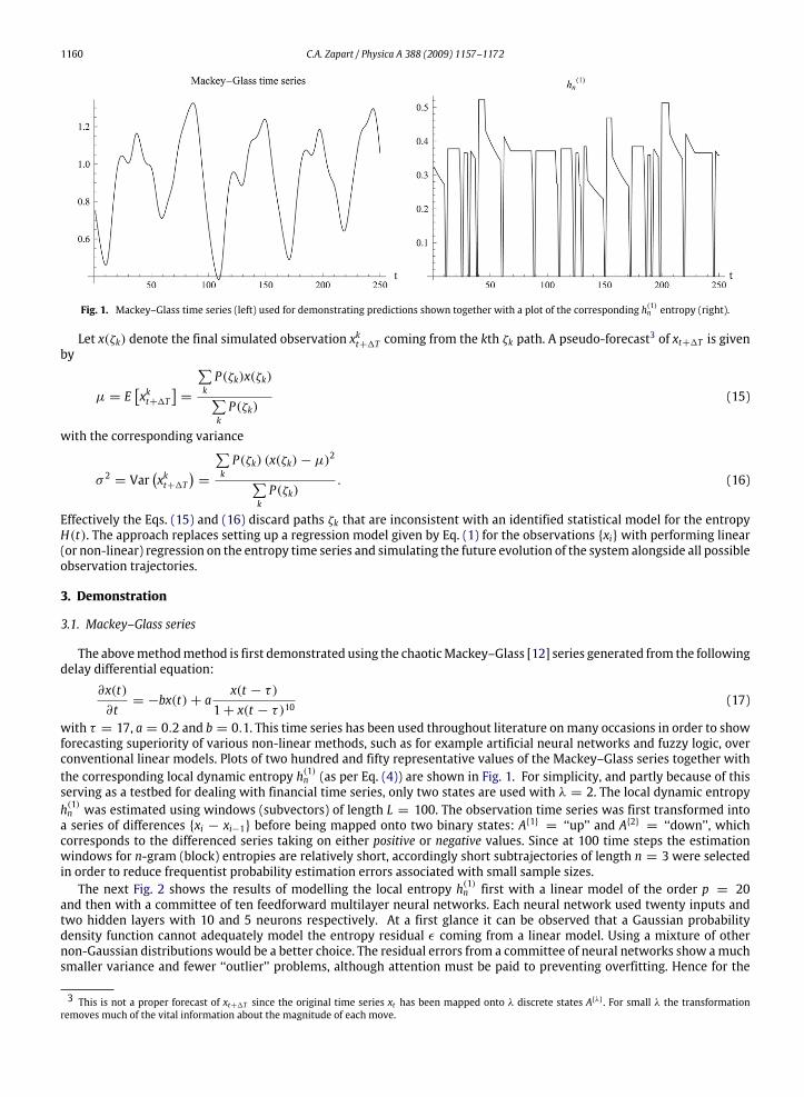
Fig. 1. Mackey–Glass time series (left) used for demonstrating predictions shown together with a plot of the corresponding h(1)n entropy (right).

Let x(ζk) denote the final simulated observation xkt+1T coming from the kth ζk path. A pseudo-forecast3 of xt+1T is given

by

µ = E[xkt+1T

]=

∑kP(ζk)x(ζk)∑kP(ζk)

(15)

with the corresponding variance

σ 2 = Var(xkt+1T

)=

∑kP(ζk) (x(ζk)− µ)2∑

kP(ζk)

. (16)

Effectively the Eqs. (15) and (16) discard paths ζk that are inconsistent with an identified statistical model for the entropyH(t). The approach replaces setting up a regression model given by Eq. (1) for the observations xiwith performing linear(or non-linear) regression on the entropy time series and simulating the future evolution of the system alongside all possibleobservation trajectories.

3. Demonstration

3.1. Mackey–Glass series

The abovemethodmethod is first demonstrated using the chaoticMackey–Glass [12] series generated from the followingdelay differential equation:

∂x(t)∂t= −bx(t)+ a

x(t − τ)1+ x(t − τ)10

(17)

with τ = 17, a = 0.2 and b = 0.1. This time series has been used throughout literature onmany occasions in order to showforecasting superiority of various non-linear methods, such as for example artificial neural networks and fuzzy logic, overconventional linear models. Plots of two hundred and fifty representative values of the Mackey–Glass series together withthe corresponding local dynamic entropy h(1)n (as per Eq. (4)) are shown in Fig. 1. For simplicity, and partly because of thisserving as a testbed for dealing with financial time series, only two states are used with λ = 2. The local dynamic entropyh(1)n was estimated using windows (subvectors) of length L = 100. The observation time series was first transformed intoa series of differences xi − xi−1 before being mapped onto two binary states: A1 = ‘‘up’’ and A2 = ‘‘down’’, whichcorresponds to the differenced series taking on either positive or negative values. Since at 100 time steps the estimationwindows for n-gram (block) entropies are relatively short, accordingly short subtrajectories of length n = 3 were selectedin order to reduce frequentist probability estimation errors associated with small sample sizes.The next Fig. 2 shows the results of modelling the local entropy h(1)n first with a linear model of the order p = 20

and then with a committee of ten feedforward multilayer neural networks. Each neural network used twenty inputs andtwo hidden layers with 10 and 5 neurons respectively. At a first glance it can be observed that a Gaussian probabilitydensity function cannot adequately model the entropy residual ε coming from a linear model. Using a mixture of othernon-Gaussian distributions would be a better choice. The residual errors from a committee of neural networks show amuchsmaller variance and fewer ‘‘outlier’’ problems, although attention must be paid to preventing overfitting. Hence for the

3 This is not a proper forecast of xt+1T since the original time series xt has been mapped onto λ discrete states Aλ . For small λ the transformationremoves much of the vital information about the magnitude of each move.

C.A. Zapart / Physica A 388 (2009) 1157–1172 1161

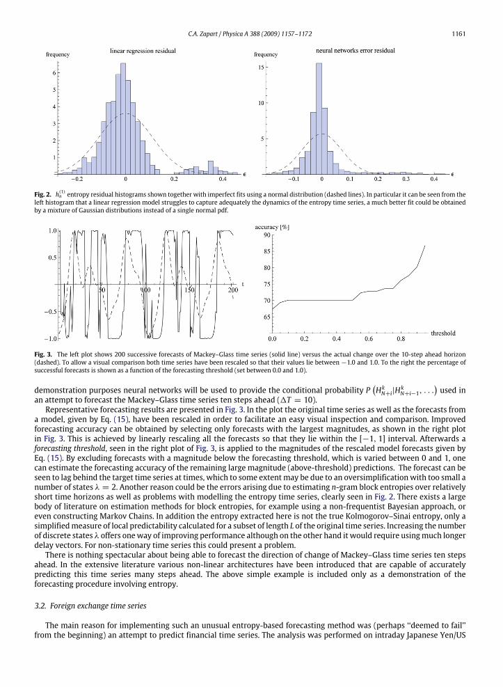
Fig. 2. h(1)n entropy residual histograms shown together with imperfect fits using a normal distribution (dashed lines). In particular it can be seen from theleft histogram that a linear regression model struggles to capture adequately the dynamics of the entropy time series, a much better fit could be obtainedby a mixture of Gaussian distributions instead of a single normal pdf.

Fig. 3. The left plot shows 200 successive forecasts of Mackey–Glass time series (solid line) versus the actual change over the 10-step ahead horizon(dashed). To allow a visual comparison both time series have been rescaled so that their values lie between −1.0 and 1.0. To the right the percentage ofsuccessful forecasts is shown as a function of the forecasting threshold (set between 0.0 and 1.0).

demonstration purposes neural networks will be used to provide the conditional probability P(HkN+i|H

kN+i−1, . . .

)used in

an attempt to forecast the Mackey–Glass time series ten steps ahead (1T = 10).Representative forecasting results are presented in Fig. 3. In the plot the original time series as well as the forecasts from

a model, given by Eq. (15), have been rescaled in order to facilitate an easy visual inspection and comparison. Improvedforecasting accuracy can be obtained by selecting only forecasts with the largest magnitudes, as shown in the right plotin Fig. 3. This is achieved by linearly rescaling all the forecasts so that they lie within the [−1, 1] interval. Afterwards aforecasting threshold, seen in the right plot of Fig. 3, is applied to the magnitudes of the rescaled model forecasts given byEq. (15). By excluding forecasts with a magnitude below the forecasting threshold, which is varied between 0 and 1, onecan estimate the forecasting accuracy of the remaining large magnitude (above-threshold) predictions. The forecast can beseen to lag behind the target time series at times, which to some extentmay be due to an oversimplificationwith too small anumber of states λ = 2. Another reason could be the errors arising due to estimating n-gram block entropies over relativelyshort time horizons as well as problems with modelling the entropy time series, clearly seen in Fig. 2. There exists a largebody of literature on estimation methods for block entropies, for example using a non-frequentist Bayesian approach, oreven constructing Markov Chains. In addition the entropy extracted here is not the true Kolmogorov–Sinai entropy, only asimplifiedmeasure of local predictability calculated for a subset of length L of the original time series. Increasing the numberof discrete states λ offers oneway of improving performance although on the other hand it would require usingmuch longerdelay vectors. For non-stationary time series this could present a problem.There is nothing spectacular about being able to forecast the direction of change of Mackey–Glass time series ten steps

ahead. In the extensive literature various non-linear architectures have been introduced that are capable of accuratelypredicting this time series many steps ahead. The above simple example is included only as a demonstration of theforecasting procedure involving entropy.

3.2. Foreign exchange time series

The main reason for implementing such an unusual entropy-based forecasting method was (perhaps ‘‘deemed to fail’’from the beginning) an attempt to predict financial time series. The analysis was performed on intraday Japanese Yen/US

1162 C.A. Zapart / Physica A 388 (2009) 1157–1172

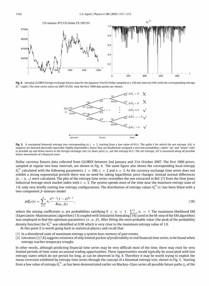
Fig. 4. Intraday GLOBEX foreign exchange futures data for the Japanese Yen/US Dollar sampled at a 120min interval (left) with the corresponding entropyh(1)n (right). The time series starts on 2007/01/02; only the first 1000 data points are shown.

Fig. 5. A conceptual binomial entropy tree corresponding to λ = 2, starting from a low value of H(t). The paths k for which the net entropy 1Hk isnegative are deemed physically impossible (highly improbable), hence they are disallowed (assigned a very low probability). Labels ‘‘up’’ and ‘‘down’’ referto possible up and down moves in the foreign exchange rate (or share price) xt , not the entropy H(t). The net entropy 1H is measured along all possiblefuture movements of a financial asset.

Dollar currency futures data collected from GLOBEX between 2nd January and 31st October 2007. The first 1000 prices,sampled at regular two hour intervals, are shown in Fig. 4. The same figure also shows the corresponding local entropyh(1)n calculated with the following parameters: L = 100, λ = 2 and n = 3. As the currency exchange time series does notexhibit a strong exponential growth there was no need for taking logarithmic price changes. Instead normal differencesxi − xi−1 were calculated. The plot of the entropy time series resembles the one extracted in Ref. [7] from the Dow JonesIndustrial Average stock market index with λ = 3. The system spends most of the time near the maximum entropy state of1.0, only very briefly visiting low entropy configurations. The distribution of entropy values h(1)n (t) has been fitted with atwo-component β-mixture model

pdfH(x) =2∑i=1

πixαi−1(1− x)βi−1

B(αi, βi), (18)

where the mixing coefficients πi are probabilities satisfying 0 ≤ πi ≤ 1,∑2i=1 πi = 1. The maximum likelihood EM

(Expectation–Maximisation) algorithm [13] coupledwith SimulatedAnnealing [14] (used in theM-step of the EMalgorithm)was employed to find the optimum parameters π, α, β. After fitting the most probable value (the peak of the probabilitydensity function) for h(1)n was identified at 0.98 which is very close to the maximum entropy value of 1.0.At this point it is worth going back to statistical physics and recall that:

(1) In a disordered state of maximum entropy a system loses memory of past events.(2) Literature [3,7,8] suggests existence of only limited pockets of predictability in real financial time series, to be foundwhenentropy reaches temporary troughs.

In other words, although predicting financial time series may be very difficult most of the time, there may exist for verylimited periods of time some occasional trading opportunities. These opportunities would typically be associated with lowentropy states which do not persist for long, as can be observed in Fig. 4. Therefore it may be worth trying to exploit themean-reversion exhibited by entropy time series through the concept of a binomial entropy tree, shown in Fig. 5. Startingfrom a low value of entropy h(1)n , as has been demonstrated earlier on Mackey–Glass series all possible future paths ζk of the

C.A. Zapart / Physica A 388 (2009) 1157–1172 1163

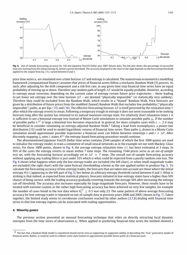
Fig. 6. Out-of-sample forecasting accuracy for 120 min Japanese Yen/US Dollar year 2007 futures data. The left plot shows the percentage of successfulforecasts starting from the initial entropyHN below a preset threshold. The accuracy displayed in the chart to the right depends on the forecasting thresholdapplied to the output from Eq. (15), varied between 0 and 1.

price time series xt are simulated over a time horizon1T and entropy is calculated. Themainstream econometricsmodellingframework (computational finance) assumes that prices of financial assets follow a stochastic RandomWalk [5] process. Assuch, after adjusting for the drift component and a risk free rate, at any given time step financial time series have an equalprobability of moving up or down. Therefore any random path of length1T would be equally probable. However, accordingto entropy mean reversion, depending on the current value of entropy certain future price trajectories – those leadingto yet lower net entropy over the time horizon 1T – are deemed ‘‘physically impossible’’ (or statistically very unlikely).Therefore they could be excluded from the Random Walk, which results in a ‘‘biased’’ Random Walk. Price forecasts aregiven by a distribution of future prices from the modified (biased) RandomWalk that excludes low probability (‘‘physicallyimpossible’’) paths, as per Eqs. (15) and (16). The effective forecasting horizon1T is itself governed by the relaxation time τafter which the entropy reverts to mean. Following a temporary trough in entropy it does not seem reasonable to be seekingforecasts long after the system has returned to its natural maximum entropy state. For relatively short relaxation times τ itis sufficient to use a binomial entropy tree instead of Monte Carlo simulations to simulate possible paths ζk. If the numberof possible paths λ1T is large a binomial tree becomes impractical. In general, for more complex cases with λ > 2 it maybe beneficial to consider simulating an entropy-adjusted Random Walk.4 Taking a lead from econophysics, a power-lawdistribution [15] could be used to model logarithmic returns of financial time series. Then paths ζk drawn in a Monte Carlosimulation would approximate possible trajectories a financial asset can follow between timesteps t and t + 1T . Afterdiscretely mapping ζk onto λ states Aλ the entropy-based forecasting procedure would continue.The aforementioned Japanese Yen/US Dollar time series contains 2544 samples of which the first 1000 quotes are used

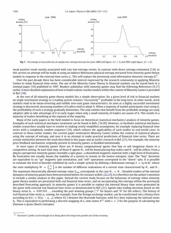
to initialise the entropy model, to train a committee of small neural networks as in the example set out with Mackey–Glassseries. For those 1000 points, shown in Fig. 4, the average entropy relaxation time 〈τ 〉 has been estimated at 3 steps. In95% of the cases the entropy reverts to mean within 7 time steps. The remaining 1544 prices serve as an out-of-sampletest set, with the forecasting horizon accordingly set to 1T = 7 steps. The overall out-of-sample forecasting accuracywithout applying any trading filters is just under 52% which is what could be expected from a purely random coin toss. TheFig. 6 shows what happens when only the low-entropy trades are included (the left chart), or when small-magnitude tradesare excluded (the right chart) with the same forecast thresholding scheme as the one applied earlier to produce Fig. 3. Tocalculate the forecasting accuracy of low-entropy trades, the forecasts that are taken into account are thosewhere the initialentropy H(t) (appearing in the left part of Fig. 5) lies below an arbitrary entropy threshold varied between 0 and 1. What isstriking is that indeed, as expected from statistical physics, forecasts initiated in low-entropy states have a higher than 50%chance of being correct, with the trading accuracy gradually reverting towards the average 50% after increasing the entropycut-off threshold. The accuracy also increases especially for large-magnitude forecasts. However, these results have to betreated with extreme caution as the rather high forecasting accuracy has been achieved on very few samples, for examplethe number of cases found in the test data where h(1)n ≤ 0.5 was only 23. The same pattern of above-average forecastingaccuracy for low-entropy trades is repeated on out-of-sample data in previous years 2006 and 2005 (shown in Fig. 7). Takentogether, the limited study seems to corroborate conclusions reached by other authors [3,7,8] dealing with financial timeseries in that low entropy regions can be associated with trading opportunities.

4. Minority games

The previous section presented an unusual forecasting technique that relies on directly extracting local dynamicentropies from the time series of observations xt . When applied to predicting financial time series the method showed a

4 The fact that a RandomWalk model is considered should not be seen as supporting its supposed validity in describing the ‘‘true’’ generative model offinancial assets. Rather, it could be used in a Monte Carlo-style fashion to approximate possible future paths of a financial asset.

1164 C.A. Zapart / Physica A 388 (2009) 1157–1172

Fig. 7. Percentage of successful out-of-sample low-entropy forecasts for years 2006 (left figure,1T = 5) and 2005 (right figure,1T = 6).

weak positive result mostly associated with rare low-entropy events. In contrast with direct entropy estimation [7,8], inthis section an attempt will be made at using an indirect Boltzmann physical entropy extracted fromminority game theorymodels in response to the external time series xt . This will replace the previously used information-theoretic entropy h

(1)n .

Over the past decade there has been considerable interest expressed by the research community in applying MinorityGames to study financial time series. The use of the Minority Game Theory in financial markets can be traced back to aseminal paper [16] published in 1997. Readers unfamiliar with minority games may find the following References [9,17]useful. Amore detailed explanation of how to build realisticmarketmodelswithin the context ofMinority Games is providedin Ref. [18].At the root of all minority game theory models lies a simple observation: for a given level of risk in financial markets

no single investment strategy or a trading system remains ‘‘excessively’’5 profitable in the long term. In other words, stockmarkets tend to be mean-reverting and exhibit zero-sum game characteristics. As soon as a highly successful investmentstrategy is discovered, increasing numbers of traders tend to adopt it. When a majority of market participants start using it,the profitability of such a strategy gradually diminishes. The only entities that benefit from the profitable strategy are earlyadopters able to take advantage of it in early stages when only a small minority of traders are aware of it. This results in aminority of traders benefiting at the expense of the majority.Many of the early papers in the field tended to focus on theoretical (statistical mechanics) analysis of minority games.

Examples of such statistical mechanics treatment can be found in Refs. [19,20]. However, to facilitate statistical mechanicsstudies researchers usually have to resolve to making overly-simplified assumptions, for example replacing financial timeseries with a completely random sequence [19], which reduces the applicability of such studies to real-world cases. Incontrast to those earlier studies, the current paper reinterprets Minority Games within the context of statistical physicsusing the concept of entropy, and uses it in an attempt to make practical predictions of financial time series. There arecertain similarities between the work described in this paper and an earlier research in Ref. [21]. For example, the minorityprice feedback mechanism, originally present in minority games, is disabled intentionally.In most types of minority games there are N binary computational agents that buy or sell imaginary shares in a

competitive setting. At each time step, of those N agents N+ will be found placing buy orders and N− will be sellers. From aphysics perspective minority games resemble a spin glass—a disordered magnetic material with a high level of frustration.By frustration one usually means the inability of a system to remain in the lowest energetic state. The ‘‘buy’’ decisionsare equivalent to an ‘‘up’’ magnetic spin orientation, and ‘‘sell’’ operations correspond to the ‘‘down’’ spin. It is possibleto estimate the level of disorder exhibited by such a simple system by defining a Boltzmann entropy S = kB lnW , wherethe state multiplicity W =

(NN+

)is the number of different realisations of a current state characterised by N+ and N−.

The maximum theoretically allowed entropy value Smax corresponds to the case N+ = N−. Detailed studies of the internaldynamics ofminority gameshave beenpresented before, for instance in Refs. [22,23]. It is therefore not the author’s intentionto include a similar analysis in this paper. Instead the current study focuses on the behaviour of entropy when minoritygame theory models are presented with real financial time series, and on incorporating this entropy within the previouslydescribed forecasting approach. In minority games it is possible to replace the internal binary time series generated bythe game with external real financial time series as demonstrated in Ref. [21]. Agents take trading decisions based on thebinary series ht = 0101101 . . . encoding the past winning groups (‘‘1’’ for buyers and ‘‘0’’ for the sellers). The history ofreal financial time series xt coming, for example, from the foreign exchange market, can be transformed into a binary formaccording to h(t) = H [xt − xt−1], where H [·] denotes the Heaviside function, with h(t) then replacing the internal seriesht . This is equivalent to performing a discrete mapping of xt onto states Aλ with λ = 2 for the purpose of calculating theShannon n-gram (block) entropies.

5 ‘‘Excessive’’ profits can be thought of as being above the long-term growth rate of the economy.

C.A. Zapart / Physica A 388 (2009) 1157–1172 1165

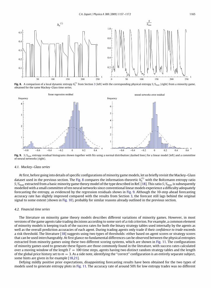
Fig. 8. A comparison of a local dynamic entropy h(1)n from Section 3 (left) with the corresponding physical entropy S/Smax (right) from a minority game,obtained for the same Mackey–Glass time series.

Fig. 9. S/Smax entropy residual histograms shown together with fits using a normal distribution (dashed lines) for a linear model (left) and a committeeof neural networks (right).

4.1. Mackey–Glass series

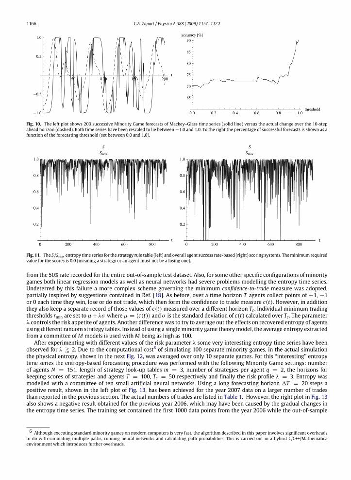
At first, before going into details of specific configurations ofminority gamemodels, let us briefly revisit theMackey–Glassdataset used in the previous section. The Fig. 8 compares the information-theoretic h(1)n with the Boltzmann entropy ratioS/Smax extracted froma basicminority game theorymodel of the type described in Ref. [18]. This ratio S/Smax is subsequentlymodelledwith a small committee of ten neural networks since conventional linearmodels experience a difficulty adequatelyforecasting the entropy, as evidenced by the regression residuals shows in Fig. 9. Although the 10-step ahead forecastingaccuracy rate has slightly improved compared with the results from Section 3, the forecast still lags behind the originalsignal to some extent (shown in Fig. 10), probably for similar reasons already outlined in the previous section.

4.2. Financial time series

The literature on minority game theory models describes different variations of minority games. However, in mostversions of the game agents take trading decisions according to some sort of a risk criterion. For example, a common elementof minority models is keeping track of the success rates for both the binary strategy tables used internally by the agents aswell as the overall prediction accuracies of each agent. During trading agents only trade if their confidence to trade exceedsa risk threshold. The literature [18] suggests using two types of thresholds: either based on agent scores or strategy scoresthat can be used interchangeably. At first glance no fundamental differences can be observed between the physical entropiesextracted from minority games using these two different scoring systems, which are shown in Fig. 11. The configurationsof minority games used to generate these figures are those commonly found in the literature, with success rates calculatedover a moving window of the length T = 100 time steps, agents having two distinct random strategy tables and the lengthof the global price history set tom = 3. As a side note, identifying the ‘‘correct’’ configuration is an entirely separate subject,some hints are given in for example [18,21].Defying mildly positive prior expectations, disappointing forecasting results have been obtained for the two types of

models used to generate entropy plots in Fig. 11. The accuracy rate of around 50% for low entropy trades was no different

1166 C.A. Zapart / Physica A 388 (2009) 1157–1172

Fig. 10. The left plot shows 200 successive Minority Game forecasts of Mackey–Glass time series (solid line) versus the actual change over the 10-stepahead horizon (dashed). Both time series have been rescaled to lie between−1.0 and 1.0. To the right the percentage of successful forecasts is shown as afunction of the forecasting threshold (set between 0.0 and 1.0).

Fig. 11. The S/Smax entropy time series for the strategy rule table (left) and overall agent success rate-based (right) scoring systems. Theminimum requiredvalue for the scores is 0.0 (meaning a strategy or an agent must not be a losing one).

from the 50% rate recorded for the entire out-of-sample test dataset. Also, for some other specific configurations of minoritygames both linear regression models as well as neural networks had severe problems modelling the entropy time series.Undeterred by this failure a more complex scheme governing the minimum confidence-to-trade measure was adopted,partially inspired by suggestions contained in Ref. [18]. As before, over a time horizon T agents collect points of +1, −1or 0 each time they win, lose or do not trade, which then form the confidence to trade measure c(t). However, in additionthey also keep a separate record of those values of c(t)measured over a different horizon Tc . Individual minimum tradingthresholds rmin are set toµ+λσ whereµ = 〈c(t)〉 and σ is the standard deviation of c(t) calculated over Tc . The parameterλ controls the risk appetite of agents. Another difference was to try to average out the effects on recovered entropy of agentsusing different random strategy tables. Instead of using a single minority game theorymodel, the average entropy extractedfrom a committee ofM models is used withM being as high as 100.After experimenting with different values of the risk parameter λ some very interesting entropy time series have been

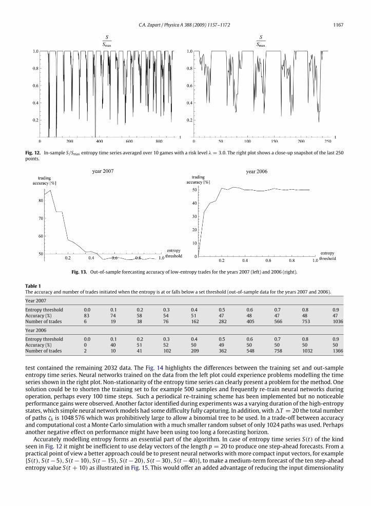
observed for λ ' 2. Due to the computational cost6 of simulating 100 separate minority games, in the actual simulationthe physical entropy, shown in the next Fig. 12, was averaged over only 10 separate games. For this ‘‘interesting’’ entropytime series the entropy-based forecasting procedure was performed with the following Minority Game settings: numberof agents N = 151, length of strategy look-up tables m = 3, number of strategies per agent q = 2, the horizons forkeeping scores of strategies and agents T = 100, Tc = 50 respectively and finally the risk profile λ = 3. Entropy wasmodelled with a committee of ten small artificial neural networks. Using a long forecasting horizon 1T = 20 steps apositive result, shown in the left plot of Fig. 13, has been achieved for the year 2007 data on a larger number of tradesthan reported in the previous section. The actual numbers of trades are listed in Table 1. However, the right plot in Fig. 13also shows a negative result obtained for the previous year 2006, which may have been caused by the gradual changes inthe entropy time series. The training set contained the first 1000 data points from the year 2006 while the out-of-sample

6 Although executing standard minority games on modern computers is very fast, the algorithm described in this paper involves significant overheadsto do with simulating multiple paths, running neural networks and calculating path probabilities. This is carried out in a hybrid C/C++/Mathematicaenvironment which introduces further overheads.

C.A. Zapart / Physica A 388 (2009) 1157–1172 1167

Fig. 12. In-sample S/Smax entropy time series averaged over 10 games with a risk level λ = 3.0. The right plot shows a close-up snapshot of the last 250points.

Fig. 13. Out-of-sample forecasting accuracy of low-entropy trades for the years 2007 (left) and 2006 (right).

Table 1The accuracy and number of trades initiated when the entropy is at or falls below a set threshold (out-of-sample data for the years 2007 and 2006).

Year 2007

Entropy threshold 0.0 0.1 0.2 0.3 0.4 0.5 0.6 0.7 0.8 0.9Accuracy (%) 83 74 58 54 51 47 48 47 48 47Number of trades 6 19 38 76 162 282 405 566 753 1036

Year 2006

Entropy threshold 0.0 0.1 0.2 0.3 0.4 0.5 0.6 0.7 0.8 0.9Accuracy (%) 0 40 51 52 50 49 50 50 50 50Number of trades 2 10 41 102 209 362 548 758 1032 1366

test contained the remaining 2032 data. The Fig. 14 highlights the differences between the training set and out-sampleentropy time series. Neural networks trained on the data from the left plot could experience problems modelling the timeseries shown in the right plot. Non-stationarity of the entropy time series can clearly present a problem for themethod. Onesolution could be to shorten the training set to for example 500 samples and frequently re-train neural networks duringoperation, perhaps every 100 time steps. Such a periodical re-training scheme has been implemented but no noticeableperformance gains were observed. Another factor identified during experiments was a varying duration of the high-entropystates, which simple neural networkmodels had some difficulty fully capturing. In addition, with1T = 20 the total numberof paths ζk is 1048576 which was prohibitively large to allow a binomial tree to be used. In a trade-off between accuracyand computational cost a Monte Carlo simulation with a much smaller random subset of only 1024 paths was used. Perhapsanother negative effect on performance might have been using too long a forecasting horizon.Accurately modelling entropy forms an essential part of the algorithm. In case of entropy time series S(t) of the kind

seen in Fig. 12 it might be inefficient to use delay vectors of the length p = 20 to produce one step-ahead forecasts. From apractical point of view a better approach could be to present neural networks withmore compact input vectors, for exampleS(t), S(t−5), S(t−10), S(t−15), S(t−20), S(t−30), S(t−40), to make amedium-term forecast of the ten step-aheadentropy value S(t + 10) as illustrated in Fig. 15. This would offer an added advantage of reducing the input dimensionality

1168 C.A. Zapart / Physica A 388 (2009) 1157–1172

Fig. 14. Changes in entropy (last 250 points) between the training set (left) and out-of-sample entropy time series (right) observed for the year 2006data set.

Fig. 15. Out-of-sample entropy time series S(t) predicted ten steps ahead. Solid line represents predictions from neural networks superimposed onto theactual time series (dashed line).

thus helping to prevent overfitting. Moreover, the path probability P(ζk) need not necessarily be given by Eq. (7) thatis perhaps more suited for ‘‘well-behaved’’ mean-reverting entropy. One could use the same forecasting horizons 1T forpredicting both entropy S(t) and the underlying financial time series xt . Then instead of using a product of conditionalprobabilities estimated from one step-ahead entropy predictions, the probability P(ζk) could be expressed as a function ofa linear correlation coefficient between the predicted and observed entire entropy paths of the length1T .After replacing one-step ahead entropy predictions with1T = 20 steps ahead forecasts utilising compact input vectors

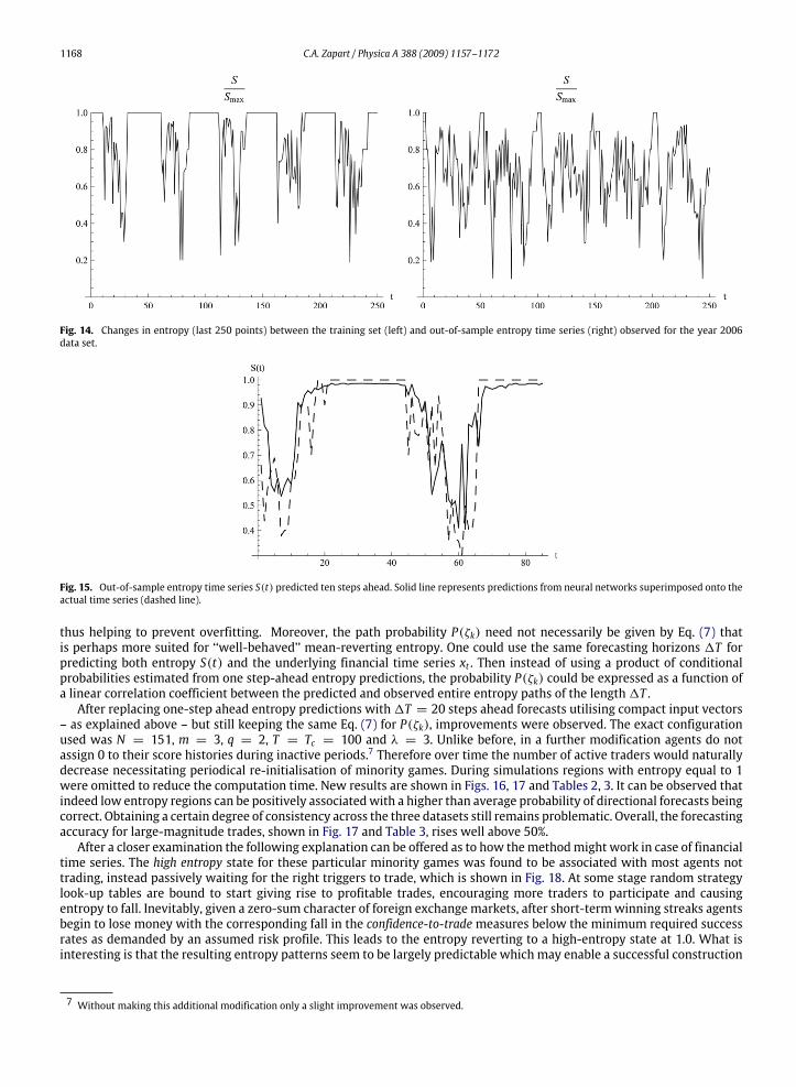
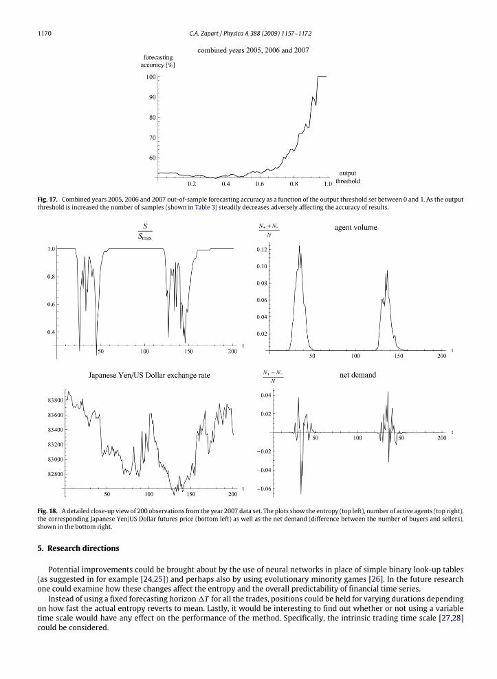
– as explained above – but still keeping the same Eq. (7) for P(ζk), improvements were observed. The exact configurationused was N = 151, m = 3, q = 2, T = Tc = 100 and λ = 3. Unlike before, in a further modification agents do notassign 0 to their score histories during inactive periods.7 Therefore over time the number of active traders would naturallydecrease necessitating periodical re-initialisation of minority games. During simulations regions with entropy equal to 1were omitted to reduce the computation time. New results are shown in Figs. 16, 17 and Tables 2, 3. It can be observed thatindeed low entropy regions can be positively associatedwith a higher than average probability of directional forecasts beingcorrect. Obtaining a certain degree of consistency across the three datasets still remains problematic. Overall, the forecastingaccuracy for large-magnitude trades, shown in Fig. 17 and Table 3, rises well above 50%.After a closer examination the following explanation can be offered as to how themethodmight work in case of financial

time series. The high entropy state for these particular minority games was found to be associated with most agents nottrading, instead passively waiting for the right triggers to trade, which is shown in Fig. 18. At some stage random strategylook-up tables are bound to start giving rise to profitable trades, encouraging more traders to participate and causingentropy to fall. Inevitably, given a zero-sum character of foreign exchange markets, after short-termwinning streaks agentsbegin to lose money with the corresponding fall in the confidence-to-trademeasures below the minimum required successrates as demanded by an assumed risk profile. This leads to the entropy reverting to a high-entropy state at 1.0. What isinteresting is that the resulting entropy patterns seem to be largely predictable which may enable a successful construction

7 Without making this additional modification only a slight improvement was observed.

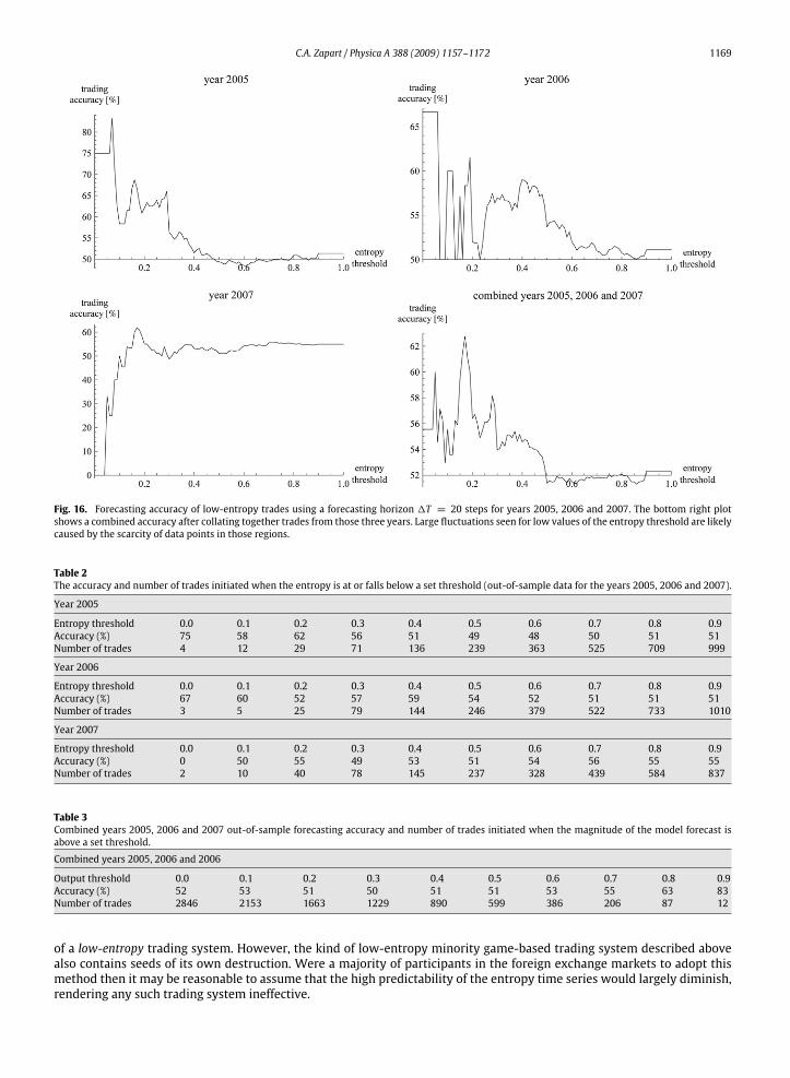
C.A. Zapart / Physica A 388 (2009) 1157–1172 1169

Fig. 16. Forecasting accuracy of low-entropy trades using a forecasting horizon 1T = 20 steps for years 2005, 2006 and 2007. The bottom right plotshows a combined accuracy after collating together trades from those three years. Large fluctuations seen for low values of the entropy threshold are likelycaused by the scarcity of data points in those regions.

Table 2The accuracy and number of trades initiated when the entropy is at or falls below a set threshold (out-of-sample data for the years 2005, 2006 and 2007).

Year 2005

Entropy threshold 0.0 0.1 0.2 0.3 0.4 0.5 0.6 0.7 0.8 0.9Accuracy (%) 75 58 62 56 51 49 48 50 51 51Number of trades 4 12 29 71 136 239 363 525 709 999

Year 2006

Entropy threshold 0.0 0.1 0.2 0.3 0.4 0.5 0.6 0.7 0.8 0.9Accuracy (%) 67 60 52 57 59 54 52 51 51 51Number of trades 3 5 25 79 144 246 379 522 733 1010

Year 2007

Entropy threshold 0.0 0.1 0.2 0.3 0.4 0.5 0.6 0.7 0.8 0.9Accuracy (%) 0 50 55 49 53 51 54 56 55 55Number of trades 2 10 40 78 145 237 328 439 584 837

Table 3Combined years 2005, 2006 and 2007 out-of-sample forecasting accuracy and number of trades initiated when the magnitude of the model forecast isabove a set threshold.

Combined years 2005, 2006 and 2006

Output threshold 0.0 0.1 0.2 0.3 0.4 0.5 0.6 0.7 0.8 0.9Accuracy (%) 52 53 51 50 51 51 53 55 63 83Number of trades 2846 2153 1663 1229 890 599 386 206 87 12

of a low-entropy trading system. However, the kind of low-entropy minority game-based trading system described abovealso contains seeds of its own destruction. Were a majority of participants in the foreign exchange markets to adopt thismethod then it may be reasonable to assume that the high predictability of the entropy time series would largely diminish,rendering any such trading system ineffective.

1170 C.A. Zapart / Physica A 388 (2009) 1157–1172

Fig. 17. Combined years 2005, 2006 and 2007 out-of-sample forecasting accuracy as a function of the output threshold set between 0 and 1. As the outputthreshold is increased the number of samples (shown in Table 3) steadily decreases adversely affecting the accuracy of results.

Fig. 18. A detailed close-up view of 200 observations from the year 2007 data set. The plots show the entropy (top left), number of active agents (top right),the corresponding Japanese Yen/US Dollar futures price (bottom left) as well as the net demand (difference between the number of buyers and sellers),shown in the bottom right.

5. Research directions

Potential improvements could be brought about by the use of neural networks in place of simple binary look-up tables(as suggested in for example [24,25]) and perhaps also by using evolutionary minority games [26]. In the future researchone could examine how these changes affect the entropy and the overall predictability of financial time series.Instead of using a fixed forecasting horizon1T for all the trades, positions could be held for varying durations depending

on how fast the actual entropy reverts to mean. Lastly, it would be interesting to find out whether or not using a variabletime scale would have any effect on the performance of the method. Specifically, the intrinsic trading time scale [27,28]could be considered.

C.A. Zapart / Physica A 388 (2009) 1157–1172 1171

6. Conclusions

The study represents an imperfect attempt to utilise entropy in the hope of being able to predict financial time series. Analternative time series forecasting method has been demonstrated which relies on building a statistical model of entropy.Instead of predicting directly the underlying time series the method first extracts the corresponding entropy, subsequentlyperforming predictions on the entropy time series.Using an information-theoretic entropy a weak trading advantage has been found in financial forecasts of foreign

exchange currency futures initiated in low entropy regions, which agrees with results from other, earlier econophysicsstudies. Conversely, predicting time series in high entropy regions is very difficult to achieve. This follows directly fromstatistical physics which teaches that in a disordered state of maximum entropy complex systems lose memory of pastevents.Established statistical time series forecasting techniques, both linear regression and non-linear neural networks, do

not take into account the physical generative aspect of financial time series. Such time series arise directly as a result ofinteractions between a large number of traders. As a consequence, from a physics point of view a much more attractiveproposition is to try to approximate the underlying processes responsible for generating the time series in the first place.Therefore the paper attempted to replace an information-theoretic entropywith a physical entropy extracted fromminoritygame theory models. According to literature [22] such models could provide a simplified approximation to the way realfinancial markets operate. One advantage of minority games is that they allow more control over the type of disorder (orcomplexitymeasure) being extracted from the time series. However, this comes at a price of having to decide how to choosethe ‘‘correct’’ model configuration. As yet there is no principled way of dealing with this issue.During the course of experiments a number of difficulties arose. Although very good forecasting results from minority

games were reported earlier in Refs. [18,21], other authors have also encountered a somewhat less positive experience [29].Overall, within the context of physical entropy the study presented in this paper offers a mixed picture of standardminoritygames. The entropy-based approach depends crucially on accurate forecasting of entropy time series. Some configurationsof minority games may result in entropy sequences that are difficult to predict. The non-stationary behaviour of entropymay also prove problematic. Optimum models used to forecast entropy need to be identified on a case-by-case basis. Afterimproving the entropy forecasting process it has been possible to obtain positive results that are consistent with statisticalphysics. However, the small size of the data sample makes the results only indicative of what can be potentially achievedafter perfecting the implementation. Greater consistency of results across different financial datasets needs to be obtainedand the failure modes need to be investigated.The multi-step ahead forecasting method outlined in this paper offers one advantage over other models that utilise

artificial stockmarkets andmultiple agents. It removes the need for having an internal price makingmechanism involved inmaking transitions between time steps from t to t+1T . However, the often large computational cost of simulating possiblefuture paths over long time horizons stipulates the need for usingMonte Carlo sampling. Comparedwith conventional linearregression models, artificial neural networks have been found more adept at modelling sometimes complex entropy timeseries.Summing up, the paper attempted to express quantitatively a qualitative claim that ‘‘low entropy regions lead to

improved predictability of financial time series’’. In doing so it makes a positive contribution towards greater acceptance ofeconophysics by the mainstream computational finance.

Acknowledgements

The authorwould like to acknowledge financial support received from the JapaneseMinistry of Education, Culture, Sports,Science and Technology. The author would also like to thank Tamami for her patience, understanding and support.

References

[1] M.P Clements, P.H Franses, N.R Swanson, Forecasting economic and financial time-series with non-linear models, International Journal of Forecasting20/2 (2004) 169–183.

[2] J.D Farmer, Physicists attempt to scale the ivory towers of finance, Computing in Science and Engineering (1999) 26–39.[3] G. A Darbellay, D. Wuertz, The entropy as a tool for analysing statistical dependencies in financial time series, Physica A 287 (2000) 429–439.[4] B. Mandelbrot, A multifractal walk down wall street, Scientific American (1999) 50–53.[5] J. Voit, The Statistical Mechanics of Financial Markets, Springer, 2005.[6] E. Cheoljun, C. Sunghoon, O. Gabjin, J. Woo-Sung, Hurst exponent and prediction based on weak-form efficient market hypothesis of stock markets,Physica A 387 (2008) 4630–4636.

[7] L. Molgedey, W. Ebeling, Local order, entropy and predictability of financial time series, European Physical Journal B-Condensed Matter and ComplexSystems 15/4 (2000) 733–737.

[8] L. Molgedey, W. Ebeling, Intraday patterns and local predictability of high-frequency financial time series, Physica A 287 (2000) 420–428.[9] E. Moro, The minority game: An introductory guide, Advances in Condensed Matter and Statistical Physics (2004).[10] C. Chatfield, The Analysis of Time Series, Chapman & Hall/CRC, 2004.[11] S. Haykin, Neural Networks, Maxwell Macmillan, 1994.[12] M.C. Mackey, L. Glass, Oscillation and chaos in physiological control systems, Science 197 (1977) 287–289.[13] A.P Dempster, N.M Laird, D.B Rubin, Maximum likelihood from incomplete data via the EM algorithm (with discussion), Journal of Royal Statistical

Society B 39 (1977) 1–38.[14] C.R Reeves, Modern Heuristic Techniques for Combinatorial Problems, Halsted Press, 1993.

1172 C.A. Zapart / Physica A 388 (2009) 1157–1172

[15] X. Gabaix, P. Gopikrishnan, V. Plerou, H.E Stanley, A theory of power-law distributions in financial market fluctuations, Nature 423 (2003) 267–270.[16] D. Challet, Y.C. Zhang, Emergence of cooperation and organisation in an evolutionary game, Physica A 246 (1997) 407.[17] D. Challet, M. Marsili, Y. Zhang, Minority Games: Interacting Agents in Financial Markets (Oxford Finance), Oxford University Press, 2005.[18] P. Jeffries, M.L. Hart, P.M. Hui, N.F. Johnson, Frommarket games to real-world markets, European Physical Journal B - Condensed Matter and Complex

Systems (2001) 493–501. Springer.[19] A. Coolen, Non-equilibrium statistical mechanics of Minority Games, in: Proceedings of Cergy 2002.[20] E. Burgos, H. Ceva, R.P.J. Perazzo, Order and disorder in the local evolutionary minority game, Physica A 354 (2005) 518–538.[21] D. Lamper, S. Howison, N.F. Johnson, Predictability of large future changes in a competitive evolving population, Advances in Condensed Matter and

Statistical Physics (2001).[22] D. Challet, M. Marsili, Y.C. Zhang, Stylized facts of financial markets and market crashes in minority games, Physica A 294 (2001) 514–524.[23] M.L. Hart, P. Jeffries, N.F. Johnson, Dynamics of the time horizon minority game, Advances in Condensed Matter and Statistical Physics (2001).[24] R. Metzler, Neural networks, game theory and time series generation, Ph.D. Dissertation, cond-mat/0212486, 2002.[25] L. Grilli, A. Sfrecola, A Neural Networks approach to Minority Game, Quaderni DSEMS, Technical Report of Dipartimento di Scienze Economiche,

Matematiche e Statistiche, Universita’ di Foggia, 2005, pp.13–2005. http://ideas.repec.org/p/ufg/qdsems/13-2005.html.[26] R. Metzler, C. Horn, Evolutionary minority game: The benefits of imitation, Advances in Condensed Matter and Statistical Physics (2002)

oai:arXiv.org:cond-mat/0109166.[27] U.A. Muller, R. Dacorogna, R.D. Davé, O.V. Pictet, R.B. Olsen, J.R. Ward, Fractals and intrinsic time — A challenge to econometricians, Opening address

of the XXXIXth International Conference of the Applied Econometrics Association, AEA, Real Time Econometrics — Submonthly Time Series, Ascona,Switzerland, 1993.

[28] E. Derman, The perception of time, risk and return during periods of speculation, Quantitative Finance 2 (2002) 282–296.[29] J.V. Andersen, D. Sornette, A mechanism for pockets of predictability in complex adaptive systems, Europhysics Letters 70 (5) (2005) 697–703.