On Enhancing 3D-FFT Performance in VASPFlorian Wende?, Martijn Marsman??, Thomas Steinke?

?Zuse Institute Berlin, Takustrasse 9, 14195 Berlin, Germany: {wende, steinke}@zib.de??Universitat Wien, Sensengasse 8, 1090 Wien, Austria: martijn.marsman@univie.ac.at

Abstract—We optimize the computation of 3D-FFT in VASP inorder to prepare the code for an efficient execution on multi- andmany-core CPUs like Intel’s Xeon Phi. Along with the transitionfrom MPI to MPI+OpenMP, library calls need to adapt tothreaded versions. One of the most time consuming componentsin VASP is 3D-FFT. Beside assessing the performance of multi-threaded calls to FFTW and Intel MKL, we investigate strategiesto improve the performance of FFT in a general sense. Weincorporate our insights and strategies for FFT computation intoa library which encapsulates FFTW and Intel MKL specifics andimplements the following features: reuse of FFT plans, composedFFTs, and the use of high bandwidth memory on Intel’s KNLXeon Phi. We will present results on a Cray-XC40 and a Cray-XC30 Xeon Phi system using synthetic benchmarks and with thelibrary integrated into VASP.

I. INTRODUCTION

The Fast Fourier Transform (FFT) is relevant to manyscientific codes. Besides those shipping with their own, maybeproblem specific, FFT implementation, many codes draw onlibrary based solutions like the widely used FFTW [1]—in-cluded within Cray’s LibSci—or Intel’s MKL. As FFT codeoptimization is close to the hardware, the integration of FFTinto codes using external libraries can be expected the “moreportable” way in the sense of maintaining the code baseover longer periods of architectural changes of the computerhardware. However, with the transition from multi-core tomany-core CPUs as well as the integration of additional layersin the memory hierarchy, like the high bandwidth memory onIntel’s upcoming Knights Landing (KNL) platform, the wayhow the FFT library itself is called from within the programneeds to be reconsidered.

For (legacy) MPI-only codes, adaptions towards MPI+X,e.g., MPI+OpenMP, require to either call into the FFT libraryfrom within a multi-threaded program context or to use amulti-threaded version of the library. In both cases the scalingof the FFT computation with the number of threads will affectthe partitioning of the execution streams into MPI ranks andthreads per rank. On Intel’s KNL with its 60+ cores and up to4 hardware threads per core, the minimization of MPI rankstogether with thread count maximization should be targeted toleverage its compute resources most effectively. In the VASPapplication (as a representative of a widely used HPC code), itis challenging to scale FFT computations beyond significantlymore than a handful of threads per MPI rank, resulting inmore than 1 rank per KNL node—with its rather low per-coreperformance and its low core frequency, MPI on the KNL canbe expected to slow down with an increasing number of MPI

ranks. As 3D FFT computation consumes massive amounts oftime for many VASP inputs, optimizing its usage within VASPis necessary in order to make the code ready not just for KNL,but for future computer platforms as well.

This paper contains the following contributions in the con-text of FFT computation on modern computer platforms:• We evaluate the threading performance of widely used

FFTW (Cray LibSci) and Intel’s MKL on a current Cray-XC40 with Intel Haswell CPUs and a Cray-XC30 XeonPhi (Knights Corner, KNC) system.

• We investigate strategies to improve the FFT performanceincluding plan reuse, composed FFT computation, skip-ping of data transpose operations between successiveFFTs, and the use of high bandwidth memory (as apreparation for Intel’s KNL).

• We introduce the C++ template library FFTLIB whichencapsulates our findings and provides them to the userin a transparent way by intercepting calls to FFTW.

Related Work: Being used in a large variety of computa-tional workflows and data processing, FFT has been subject tooptimizations for a long time already. It is well-known that forDensity Functional Theory (DFT) computations with plane-wave basis sets, the 3D-FFT is one of the time-critical compu-tational steps [8]. For computations on moderately sized grids,as is the case for many VASP inputs, for instance, domain-specific optimized FFTs exist. Our work focuses on optimizingthe 3D-FFT for plane-wave DFT methods. With peta-scalecompute systems available, most of the related work is focusedon scalable, distributed 3D-FFT implementations [4], [6]. Inthis paper, we focus on on-node 3D-FFT computation. Ourfindings regarding composed FFT computation, however, canbe used in the context of distributed 3D-FFT computation aswell.

II. FFT COMPUTATION WITH FFTW (LIBSCI) AND MKL

A. The Fast Fourier Transform

The FFT is an efficient way to calculate the Fourier Trans-form [9]

f (k) : f (kn) =N−1

∑j=0

f (x j)e2πinj

N , kn =2nπ

L, n = 0, . . . ,N−1

(1)of a periodic function f (x) with period L, defined on N discretepoints x = {x j = j L

N | j = 0, . . . ,N − 1}, with computationalcomplexity O(N log2(N)) opposed to O(N2) in case of doingit straightforwardly. FFT uses the fact that eikx has the same

value for different combinations of x and k, thereby reducingthe number of computational steps.

Note that Eq. 1 describes the one-dimensional FFT of f (x)(or 1D-FFT for short). However, n-dimensional FFTs can bethought of as being composed of n successive 1D-FFTs.

B. FFTW and MKL

Both FFTW [1] and Intel MKL provide to the user acommon C and Fortran interface for 1D-, 2D- and 3D-FFTcomputation on complex and real data. On Cray machines,FFTW (possibly with some Cray specific optimizations) isaccessible through LibSci. Additionally, MKL provides an ex-tended feature set that is available through its DFTI interface,which is a superset of what is accessible through its FFTWcompatibility layer. All of these libraries will be available onIntel’s KNL platform due to its x86 compatibility which allowsfor non-Intel software stacks. Users hence will have the choiceto either use FFTW (through LibSci) or MKL on KNL.

In this paper, we use the following FFT library versions:a self-compiled version of FFTW,1 a Cray-optimized versionof FFTW (rev. 3.3.4) through LibSci 13.2.0, and FFT throughIntel’s FFTW wrappers coming with MKL 11.3.2. Generalcode compilation happened with the Intel 16.0.2 (20160204)C/C++/Fortran compiler. We use Cray’s iobuf library (rev.2.0.6) and craype-hugepages8M. Our hardware configu-ration comprises: Cray-XC40 compute nodes with dual-socketIntel Xeon E5-2680v3 Haswell CPUs (24 cores per node, andcores clocked at 1.9 GHz—AVX base frequency), and a Cray-XC30 test system with Intel Xeon Phi 5120D coprocessors(59 cores per device, and 4-way hardware multi-threading percore).

Using the FFTW Interface: The usual pattern when callingFFTW (or MKL through its FFTW interface) is as follows:

0. (optional) Initialize threading viafftw_init_threads() andfftw_plan_with_nthreads(nthreads).

1. Create plans for FFT computations, e.g., viafftw_plan p=fftw_plan_dft_3d(..).

2. Perform FFT computation using that plan (as oftenas needed) viafffw_execute(p) orfftw_execute_dft(p,in,out).

3. Clean up plans viafftw_plan_destroy(p) andfftw_cleanup() or

1The source code has been taken from the official FFTW GitHub reposi-tory https://github.com/FFTW/FFTW, and has been compiled usingIntel’s C/C++/Fortran compiler 16.0.2 (20160204) with configure options--enable-avx2 --enable-fma --enable-openmp for HaswellCPU, and --enable-kcvi --enable -fma --enable-openmp forIntel Xeon Phi (KNC). Compile options: -O3 and -xcore-avx2 forHaswell and -mmic for Xeon Phi (KNC). For Xeon Phi, we additionallybuilt the official FFTW library (rev. 3.3.4) due to significantly reduced plannerperformance of FFTW from GitHub—not so on Haswell. However, the officialFFTW library (rev. 3.3.4) does not incorporate Xeon Phi optimizations andhence gives poor performance.

fftw_cleanup_threads().

Before the actual FFT computation, a plan p needs to becreated. Any plan p can be used as often as needed until eitherfftw_plan_destroy(p), fftw_cleanup() or fftw_cleanup_threads() is called. It is recommended to useplans as often as possible to amortize for their creation costs.

Plan creation with FFTW can happen with differently ex-pensive planner schemes:

FFTW_ESTIMATE (cheap),FFTW_MEASURE (expensive),FFTW_PATIENT (more expensive) andFFTW_EXHAUSTIVE (most expensive).

Except for FFTW_ESTIMATE plan creation involves testingdifferent FFT algorithms together with runtime measurementsto achieve best performance on the target platform. With MKL,these schemes can be specified for compatibility reasons, butnone of them affect the internal planner.

To speed up the plan creation step, FFTW implements theso-called “wisdom” feature which is used when planning withFFTW_MEASURE or any of the more expensive schemes. Foreach plan requested from FFTW, an internal data structureis created that holds a “minimal” set of information for fastplan recreation in case of compatible successive requests.When doing lots of FFTs for certain grid geometries, it isrecommended for each of them to first plan with any of theexpensive schemes and then to use the same scheme againor FFTW_ESTIMATE. Wisdom then will be used to get the“good” plans much faster:

// first planner call: expensivep=fftw_plan_dft_3d(64,72,68,in,out,

FFTW_FORWARD,FFTW_MEASURE)

// successive planner call(s): wisdom is usedp=fftw_plan_dft_3d(64,72,68,in,out,

FFTW_FORWARD,FFTW_MEASURE).

C. 3D-FFT in VASP (Initial Setup)

In the VASP application the following pattern is used for allkinds of FFT computation: “create plan – execute(n) – destroyplan,” where n = 1 in most cases. Table. I summarizes forone particular input (PdO2: Palladiumdioxide on a Paladiumserface) the total execution time of VASP using 24 MPI rankson 4 Cray-XC40 compute nodes. Each MPI rank uses either 1or 4 OpenMP threads, with all MPI ranks and threads evenlydistributed across the two CPU sockets per node.

For runs with MKL, the 3D-FFT performance increases byabout factor 2.2 when using 4 instead of 1 OpenMP thread.With FFTW, we observe the opposite, that is, the time spentin 3D-FFT computation increases with the number of threads.The effective performance loss can be traced to the plannerof the FFTW library—VASP strictly follows the proposedproceeding: plan with FFTW_MEASURE in the first instance,and then use FFTW_ESTIMATE [1]. The 3D-FFT executiontime, on the other hand, decreases with the number of threads.

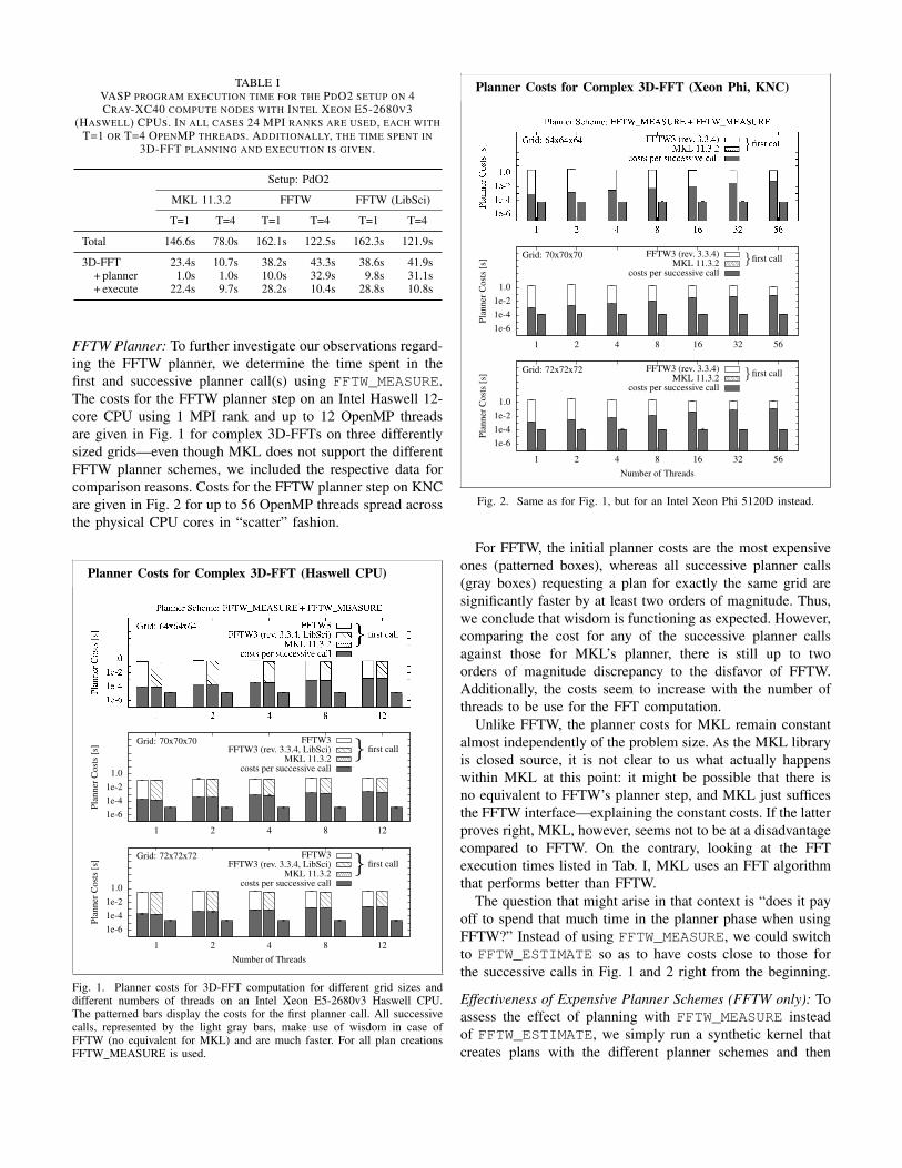
TABLE IVASP PROGRAM EXECUTION TIME FOR THE PDO2 SETUP ON 4CRAY-XC40 COMPUTE NODES WITH INTEL XEON E5-2680V3

(HASWELL) CPUS. IN ALL CASES 24 MPI RANKS ARE USED, EACH WITHT=1 OR T=4 OPENMP THREADS. ADDITIONALLY, THE TIME SPENT IN

3D-FFT PLANNING AND EXECUTION IS GIVEN.

Setup: PdO2

MKL 11.3.2 FFTW FFTW (LibSci)

T=1 T=4 T=1 T=4 T=1 T=4

Total 146.6s 78.0s 162.1s 122.5s 162.3s 121.9s

3D-FFT 23.4s 10.7s 38.2s 43.3s 38.6s 41.9s+ planner 1.0s 1.0s 10.0s 32.9s 9.8s 31.1s+ execute 22.4s 9.7s 28.2s 10.4s 28.8s 10.8s

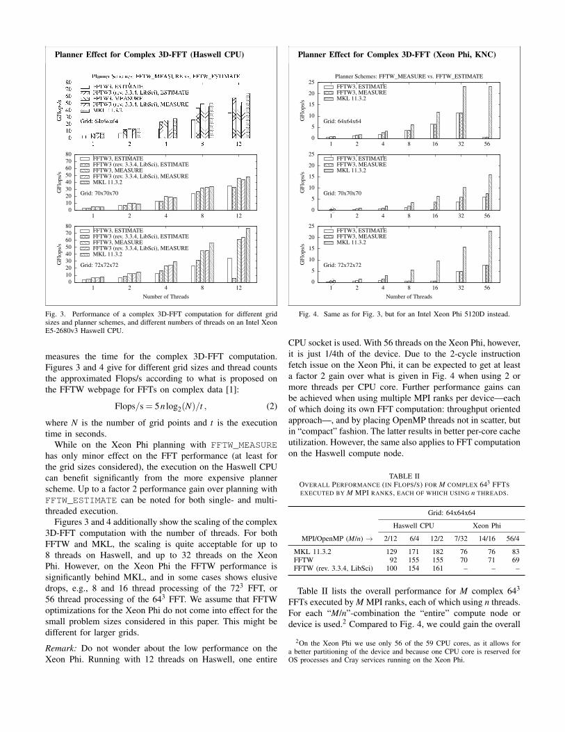
FFTW Planner: To further investigate our observations regard-ing the FFTW planner, we determine the time spent in thefirst and successive planner call(s) using FFTW_MEASURE.The costs for the FFTW planner step on an Intel Haswell 12-core CPU using 1 MPI rank and up to 12 OpenMP threadsare given in Fig. 1 for complex 3D-FFTs on three differentlysized grids—even though MKL does not support the differentFFTW planner schemes, we included the respective data forcomparison reasons. Costs for the FFTW planner step on KNCare given in Fig. 2 for up to 56 OpenMP threads spread acrossthe physical CPU cores in “scatter” fashion.

Planner Costs for Complex 3D-FFT (Haswell CPU)

1e-61e-41e-2

1.0

1 2 4 8 12

Plan

nerC

osts

[s]

Number of Threads

Planner Scheme: FFTW_MEASURE + FFTW_MEASURE

Grid: 70x70x70 } first callFFTW3

FFTW3 (rev. 3.3.4, LibSci)MKL 11.3.2

costs per successive call

1e-61e-41e-2

1.0

1 2 4 8 12

Plan

nerC

osts

[s]

Number of Threads

Planner Scheme: FFTW_MEASURE + FFTW_MEASURE

Grid: 72x72x72 } first callFFTW3

FFTW3 (rev. 3.3.4, LibSci)MKL 11.3.2

costs per successive call

Fig. 1. Planner costs for 3D-FFT computation for different grid sizes anddifferent numbers of threads on an Intel Xeon E5-2680v3 Haswell CPU.The patterned bars display the costs for the first planner call. All successivecalls, represented by the light gray bars, make use of wisdom in case ofFFTW (no equivalent for MKL) and are much faster. For all plan creationsFFTW MEASURE is used.

Planner Costs for Complex 3D-FFT (Xeon Phi, KNC)

1e-61e-41e-2

1.0

1 2 4 8 16 32 56

Plan

nerC

osts

[s]

Number of Threads

Planner Scheme: FFTW_MEASURE + FFTW_MEASURE

Grid: 70x70x70 }first callFFTW3 (rev. 3.3.4)MKL 11.3.2

costs per successive call

1e-61e-41e-2

1.0

1 2 4 8 16 32 56

Plan

nerC

osts

[s]

Number of Threads

Planner Scheme: FFTW_MEASURE + FFTW_MEASURE

Grid: 72x72x72 }first callFFTW3 (rev. 3.3.4)MKL 11.3.2

costs per successive call

Fig. 2. Same as for Fig. 1, but for an Intel Xeon Phi 5120D instead.

For FFTW, the initial planner costs are the most expensiveones (patterned boxes), whereas all successive planner calls(gray boxes) requesting a plan for exactly the same grid aresignificantly faster by at least two orders of magnitude. Thus,we conclude that wisdom is functioning as expected. However,comparing the cost for any of the successive planner callsagainst those for MKL’s planner, there is still up to twoorders of magnitude discrepancy to the disfavor of FFTW.Additionally, the costs seem to increase with the number ofthreads to be use for the FFT computation.

Unlike FFTW, the planner costs for MKL remain constantalmost independently of the problem size. As the MKL libraryis closed source, it is not clear to us what actually happenswithin MKL at this point: it might be possible that there isno equivalent to FFTW’s planner step, and MKL just sufficesthe FFTW interface—explaining the constant costs. If the latterproves right, MKL, however, seems not to be at a disadvantagecompared to FFTW. On the contrary, looking at the FFTexecution times listed in Tab. I, MKL uses an FFT algorithmthat performs better than FFTW.

The question that might arise in that context is “does it payoff to spend that much time in the planner phase when usingFFTW?” Instead of using FFTW_MEASURE, we could switchto FFTW_ESTIMATE so as to have costs close to those forthe successive calls in Fig. 1 and 2 right from the beginning.

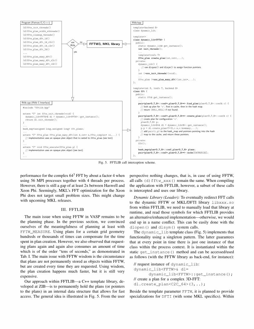
Effectiveness of Expensive Planner Schemes (FFTW only): Toassess the effect of planning with FFTW_MEASURE insteadof FFTW_ESTIMATE, we simply run a synthetic kernel thatcreates plans with the different planner schemes and then

Planner Effect for Complex 3D-FFT (Haswell CPU)

01020304050607080

1 2 4 8 12

GFl

ops/

s

Number of Threads

Planner Schemes: FFTW_MEASURE vs. FFTW_ESTIMATE

Grid: 70x70x70

FFTW3, ESTIMATEFFTW3 (rev. 3.3.4, LibSci), ESTIMATEFFTW3, MEASUREFFTW3 (rev. 3.3.4, LibSci), MEASUREMKL 11.3.2

01020304050607080

1 2 4 8 12

GFl

ops/

s

Number of Threads

Planner Schemes: FFTW_MEASURE vs. FFTW_ESTIMATE

Grid: 72x72x72

FFTW3, ESTIMATEFFTW3 (rev. 3.3.4, LibSci), ESTIMATEFFTW3, MEASUREFFTW3 (rev. 3.3.4, LibSci), MEASUREMKL 11.3.2

Fig. 3. Performance of a complex 3D-FFT computation for different gridsizes and planner schemes, and different numbers of threads on an Intel XeonE5-2680v3 Haswell CPU.

measures the time for the complex 3D-FFT computation.Figures 3 and 4 give for different grid sizes and thread countsthe approximated Flops/s according to what is proposed onthe FFTW webpage for FFTs on complex data [1]:

Flops/s = 5n log2(N)/t , (2)

where N is the number of grid points and t is the executiontime in seconds.

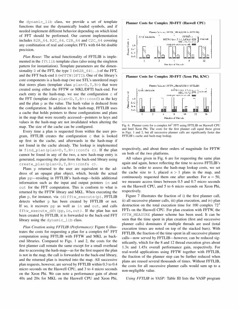
While on the Xeon Phi planning with FFTW_MEASUREhas only minor effect on the FFT performance (at least forthe grid sizes considered), the execution on the Haswell CPUcan benefit significantly from the more expensive plannerscheme. Up to a factor 2 performance gain over planning withFFTW_ESTIMATE can be noted for both single- and multi-threaded execution.

Figures 3 and 4 additionally show the scaling of the complex3D-FFT computation with the number of threads. For bothFFTW and MKL, the scaling is quite acceptable for up to8 threads on Haswell, and up to 32 threads on the XeonPhi. However, on the Xeon Phi the FFTW performance issignificantly behind MKL, and in some cases shows elusivedrops, e.g., 8 and 16 thread processing of the 723 FFT, or56 thread processing of the 643 FFT. We assume that FFTWoptimizations for the Xeon Phi do not come into effect for thesmall problem sizes considered in this paper. This might bedifferent for larger grids.

Remark: Do not wonder about the low performance on theXeon Phi. Running with 12 threads on Haswell, one entire

Planner Effect for Complex 3D-FFT (Xeon Phi, KNC)

0

5

10

15

20

25

1 2 4 8 16 32 56

GFl

ops/

s

Number of Threads

Planner Schemes: FFTW_MEASURE vs. FFTW_ESTIMATE

Grid: 64x64x64

FFTW3, ESTIMATEFFTW3, MEASUREMKL 11.3.2

0

5

10

15

20

25

1 2 4 8 16 32 56

GFl

ops/

s

Number of Threads

Planner Schemes: FFTW_MEASURE vs. FFTW_ESTIMATE

Grid: 70x70x70

FFTW3, ESTIMATEFFTW3, MEASUREMKL 11.3.2

0

5

10

15

20

25

1 2 4 8 16 32 56

GFl

ops/

sNumber of Threads

Planner Schemes: FFTW_MEASURE vs. FFTW_ESTIMATE

Grid: 72x72x72

FFTW3, ESTIMATEFFTW3, MEASUREMKL 11.3.2

Fig. 4. Same as for Fig. 3, but for an Intel Xeon Phi 5120D instead.

CPU socket is used. With 56 threads on the Xeon Phi, however,it is just 1/4th of the device. Due to the 2-cycle instructionfetch issue on the Xeon Phi, it can be expected to get at leasta factor 2 gain over what is given in Fig. 4 when using 2 ormore threads per CPU core. Further performance gains canbe achieved when using multiple MPI ranks per device—eachof which doing its own FFT computation: throughput orientedapproach—, and by placing OpenMP threads not in scatter, butin “compact” fashion. The latter results in better per-core cacheutilization. However, the same also applies to FFT computationon the Haswell compute node.

TABLE IIOVERALL PERFORMANCE (IN FLOPS/S) FOR M COMPLEX 643 FFTSEXECUTED BY M MPI RANKS, EACH OF WHICH USING n THREADS.

Grid: 64x64x64

Haswell CPU Xeon Phi

MPI/OpenMP (M/n) → 2/12 6/4 12/2 7/32 14/16 56/4

MKL 11.3.2 129 171 182 76 76 83FFTW 92 155 155 70 71 69FFTW (rev. 3.3.4, LibSci) 100 154 161 – – –

Table II lists the overall performance for M complex 643

FFTs executed by M MPI ranks, each of which using n threads.For each “M/n”-combination the “entire” compute node ordevice is used.2 Compared to Fig. 4, we could gain the overall

2On the Xeon Phi we use only 56 of the 59 CPU cores, as it allows fora better partitioning of the device and because one CPU core is reserved forOS processes and Cray services running on the Xeon Phi.

(d)fftw_init_threads()(d)fftw_plan_width_nthreads()

(d)fftw_plan_dft_1d()(d)fftw_plan_dft_1d_r2c()(d)fftw_plan_dft_1d_c2r()(d)fftw_plan_dft_2d()

(d)fftw_plan_many_dft()(d)fftw_plan_many_dft_r2c()(d)fftw_plan_many_dft_c2r()

(d)fftw_cleanup_threads()

...

template<int D, trafo T, backend B>class fft { public: static fft& get_instance(); ... pair<plan<D,T,B>::conf*,plan<D,T,B>*> find_plan(plan<D,T,B>::conf& c) { // look up plan for 'c', first in cache, then in the hash map. // return (NULL,NULL) if not found. } pair<plan<D,T,B>::conf*,plan<D,T,B>*> create_plan(plan<D,T,B>::conf& c) { // create plan for configuration 'c'. plan<D,T,B> p; dynamic_lib<B>& dl = dynamic_lib<B>::get_instance(); p.p = dl.create_plan<T>(D,c.n,c.howmany,...); // add pair(c,p) to the hash_map and pointers pointing into the hash // map to the cache, and return these pointers. } private: fft(); ... hash_map<plan<D,T,B>::conf,plan<D,T,B> plans; pair<plan<D,T,B>::conf*,plan<D,T,B>*> cache[CACHESIZE];};

template<backend B>class dynamic_lib;

template<>class dynamic_lib<FFTW> { public: static dynamic_lib& get_instance(); int init_threads(); ... template<trafo T> fftw_plan create_plan(int,int*,...); private: dynamic_lib() { // use dlopen() and dlsym() to assign function pointers. } int (*xxx_init_threads)(void); ... fftw_plan (*xxx_plan_many_dft)(int,int*,...);};

Program (Fortran/C/C++) fftlib.hpp

#include "fftlib.hpp"

extern "C" int fftw_init_threads(void) { dynamic_lib<FFTW>& dl = dynamic_lib<FFTW>::get_instance(); return dl.init_threads();}...hash_map<unsigned long,unsigned long> fft_plans;...extern "C" fftw_plan fftw_plan_many_dft(int d,int* n,fftw_complex* in,...) { // implementation uses an opaque plan object that is casted to fftw_plan (see text) }...extern "C" void fftw_execute(fftw_plan p) { // implementation uses an opaque plan object (see text)}...

fftlib.cpp (fftlib C-Interface)

FFTW3, MKL libraryuse fftlib

no

yes

Fig. 5. FFTLIB call interception scheme.

performance for the complex 643 FFT by about a factor 4 whenusing 56 MPI processes together with 4 threads per process.However, there is still a gap of at least 2x between Haswell andXeon Phi. Seemingly, MKL’s FFT optimization for the XeonPhi does not target small problem sizes. This might changewith upcoming MKL releases.

III. FFTLIB

The main issue when using FFTW in VASP remains to bethe planning phase. In the previous section, we convincedourselves of the meaningfulness of planning at least withFFTW_MEASURE. Using plans for a certain grid geometryhundreds or thousands of times can compensate for the timespent in plan creation. However, we also observed that request-ing plans again and again also consumes an amount of timewhich is of the order “tens of seconds,” as demonstrated inTab. I. The main issue with FFTW wisdom is the circumstancethat plans are not permanently stored as objects within FFTW,but are created every time they are requested. Using wisdom,the plan creation happens much faster, but it is still veryexpensive.

Our approach within FFTLIB—a C++ template library, de-veloped at ZIB—is to permanently hold the plans (or pointersto the plans) in an internal data structure that allows for fastaccess. The general idea is illustrated in Fig. 5. From the user

perspective nothing changes, that is, in case of using FFTW,all calls (d)fftw_xxx() remain the same. When compilingthe application with FFTLIB, however, a subset of these callsis intercepted and uses our library.

Dynamic Library (Loader): To eventually redirect FFT callsto the dynamic FFTW or MKL/DFTI library libxxx.sofrom within FFTLIB, we need to manually load that library atruntime, and read those symbols for which FFTLIB providesan alternative/enhanced implementation—otherwise, we wouldend up in a name conflict. This can be easily done with thedlopen() and dlsym() system calls.

The dynamic_lib template class (Fig. 5) implements thatfunctionality using a singleton pattern. The latter guaranteesthat at every point in time there is just one instance of thatclass within the process context. It is instantiated within thestatic get_instance() method and can be accessed/usedas follows (with the FFTW library as back-end, for instance):

// request instance of dynamic_lib:dynamic_lib<FFTW>& dl=

dynamic_lib<FFTW>::get_instance();// create a plan for a complex 3D-FFT:dl.create_plan<C2C_64>(3,..);

Beside the template parameter FFTW, it is planned to providespecializations for DFTI (with some MKL specifics). Within

the dynamic_lib class, we provide a set of templatefunctions that use the dynamically loaded symbols, and ifneeded implement different behavior depending on which kindof FFT should be performed. Our current implementationincludes R2R_64, R2C_64, C2R_64 and C2C_64 coveringany combination of real and complex FFTs with 64-bit doubleprecision.

Plan Reuse: The actual functionality of FFTLIB is imple-mented in the fftlib template class (also using the singletonpattern for instantiation). Template parameters are the dimen-sionality D of the FFT, the type T (=R2R_64|. . .) of the FFT,and the FFT back-end B (=FFTW|DFTI). One of the library’score components is a hash-map (we use STL’s unordered map)that stores plans (template class plan<D,T,B>) that werecreated using either the FFTW or MKL/DFTI back-end. Foreach entry in the hash-map, we use the configuration c ofthe FFT (template class plan<D,T,B>::conf) as the keyand the plan p as the value. The hash value is deduced fromthe configuration. In addition to the hash-map, FFTLIB usesa cache that holds pointers to those configurations and plansin the map that were recently accessed—pointers to keys andvalues in the hash-map are not invalidated when altering themap. The size of the cache can be configured.

Every time a plan is requested from within the user pro-gram, FFTLIB creates the configuration c that is lookedup first in the cache, and afterwards in the hash-map ifnot found in the cache already. The lookup is implementedin find_plan(plan<D,T,B>::conf& c). If the plancannot be found in any of the two, a new hash-map entry isgenerated, requesting the plan from the back-end library usingcreate_plan(plan<D,T,B>::conf& c).

Plans p returned to the user are equivalent to the ad-dress of an opaque plan object, which, beside the actualplan pp—residing in FFTLIB’s hash-map—holds additionalinformation such as the input and output pointers in andout for the FFT computation. This is conform to what isreturned by the FFTW library and MKL. When executing theplan p, for instance, via (d)fftw_execute(p), FFTLIBdetects whether p has been created by FFTLIB or not.If so, it recovers pp as well as in and out, and callsfftw_execute_dft(pp,in,out). If the plan has notbeen created by FFTLIB, it is forwarded to the back-end FFTlibrary using the dynamic_lib class.

Plan Creation using FFTLIB (Performance): Figure 6 illus-trates the costs for requesting a plan for a complex 643 FFTcomputation using FFTLIB with FFTW and MKL as back-end libraries. Compared to Figs. 1 and 2, the costs for thefirst planner call remain the same except for a small overheaddue to accessing the hash-map—as for the first request the planis not in the map, the call is forwarded to the back-end library,and the returned plan is inserted into the map. All successiveplan requests, however, are served by FFTLIB within 0.3 to 0.4micro seconds on the Haswell CPU, and 3 to 4 micro secondson the Xeon Phi. We can note a performance gain of about40x and 20x for MKL on the Haswell CPU and Xeon Phi,

Planner Costs for Complex 3D-FFT (Haswell CPU)

Planner Costs for Complex 3D-FFT (Xeon Phi, KNC)

Fig. 6. Planner costs for a complex 643 FFT using FFTLIB on Haswell CPUand Intel Xeon Phi. The costs for the first planner call equal those givenin Figs. 1 and 2, but all successive planner calls are significantly faster dueFFTLIB’s cache and hash-map lookup.

respectively, and about three orders of magnitude for FFTWon both of the two platforms.

All values given in Fig. 6 are for requesting the same planagain and again, hence reflecting the time to access FFTLIB’scache. In order to assess the hash-map lookup costs, we setthe cache size to 1, placed n > 1 plans in the map, andcontinuously requested them one after another. For n = 50,we measure access times between 0.5 and 0.7 micro secondson the Haswell CPU, and 5 to 6 micro seconds on Xeon Phi,respectively.

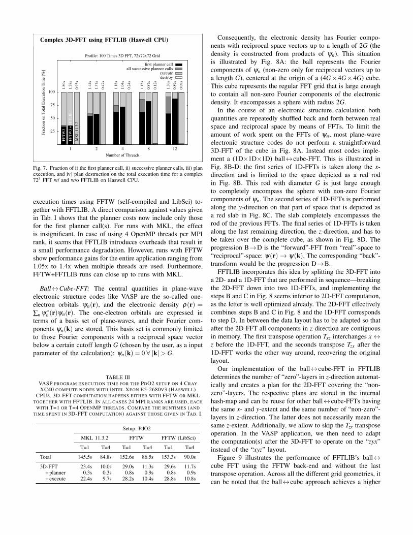
Figure 7 illustrates the fraction of i) the first planner call,ii) all successive planner calls, iii) plan execution, and iv) plandestruction on the total execution time for 100 complex 723

FFTs on the Haswell CPU. For plan creation with FFTW, theFFTW_MEASURE planner scheme has been used. It can beseen that the time spent in plan creation (first and successiveplanner calls) dominates if multiple threads are used (totalexecution times are noted on top of the stacked bars). WithFFTLIB, the fraction of the time spent in all successive plannercalls—now served by FFTLIB—however, can be reduced sig-nificantly, which for the 8 and 12 thread execution gives about1.3x and 1.45x overall performance gain, respectively. Forreal-world applications using FFTW together with FFTLIB,the fraction of the planner step can be further reduced whenplans are reused several thousands of times. Without FFTLIB,the costs for all successive planner calls would sum up to anon-negligible value.

Using FFTLIB in VASP: Table III lists the VASP program

Complex 3D-FFT using FFTLIB (Haswell CPU)

25

50

75

100

1 2 4 8 12

Frac

tion

onTo

talE

xecu

tion

Tim

e[%

]

Number of Threads

Profile: 100 Times 3D FFT, 72x72x72 Grid

1.80

s

1.78

s

0.93

s

1.44

s

1.37

s

0.47

s

1.18

s

1.04

s

0.24

s

1.15

s

0.87

s

0.12

s

1.30

s

0.89

s

0.09

s

destroyexecute

all successive planner callsfirst planner call

FFT

W3

FFT

W3

+FF

TL

IB

MK

L11

.3.2

Fig. 7. Fraction of i) the first planner call, ii) successive planner calls, iii) planexecution, and iv) plan destruction on the total execution time for a complex723 FFT w/ and w/o FFTLIB on Haswell CPU.

execution times using FFTW (self-compiled and LibSci) to-gether with FFTLIB. A direct comparison against values givenin Tab. I shows that the planner costs now include only thosefor the first planner call(s). For runs with MKL, the effectis insignificant. In case of using 4 OpenMP threads per MPIrank, it seems that FFTLIB introduces overheads that result ina small performance degradation. However, runs with FFTWshow performance gains for the entire application ranging from1.05x to 1.4x when multiple threads are used. Furthermore,FFTW+FFTLIB runs can close up to runs with MKL.

Ball↔Cube-FFT: The central quantities in plane-waveelectronic structure codes like VASP are the so-called one-electron orbitals ψn(r), and the electronic density ρ(r) =∑n ψ∗n (r)ψn(r). The one-electron orbitals are expressed interms of a basis set of plane-waves, and their Fourier com-ponents ψn(k) are stored. This basis set is commonly limitedto those Fourier components with a reciprocal space vectorbelow a certain cutoff length G (chosen by the user, as a inputparameter of the calculation): ψn(k) = 0 ∀ |k|> G.

TABLE IIIVASP PROGRAM EXECUTION TIME FOR THE PDO2 SETUP ON 4 CRAYXC40 COMPUTE NODES WITH INTEL XEON E5-2680V3 (HASWELL)

CPUS. 3D-FFT COMPUTATION HAPPENS EITHER WITH FFTW OR MKLTOGETHER WITH FFTLIB. IN ALL CASES 24 MPI RANKS ARE USED, EACH

WITH T=1 OR T=4 OPENMP THREADS. COMPARE THE RUNTIMES (ANDTIME SPENT IN 3D-FFT COMPUTATION) AGAINST THOSE GIVEN IN TAB. I.

Setup: PdO2

MKL 11.3.2 FFTW FFTW (LibSci)

T=1 T=4 T=1 T=4 T=1 T=4

Total 145.5s 84.8s 152.6s 86.5s 153.3s 90.0s

3D-FFT 23.4s 10.0s 29.0s 11.3s 29.6s 11.7s+ planner 0.3s 0.3s 0.8s 0.9s 0.8s 0.9s+ execute 22.4s 9.7s 28.2s 10.4s 28.8s 10.8s

Consequently, the electronic density has Fourier compo-nents with reciprocal space vectors up to a length of 2G (thedensity is constructed from products of ψn). This situationis illustrated by Fig. 8A: the ball represents the Fouriercomponents of ψn (non-zero only for reciprocal vectors up toa length G), centered at the origin of a (4G×4G×4G) cube.This cube represents the regular FFT grid that is large enoughto contain all non-zero Fourier components of the electronicdensity. It encompasses a sphere with radius 2G.

In the course of an electronic structure calculation bothquantities are repeatedly shuffled back and forth between realspace and reciprocal space by means of FFTs. To limit theamount of work spent on the FFTs of ψn, most plane-waveelectronic structure codes do not perform a straightforward3D-FFT of the cube in Fig. 8A. Instead most codes imple-ment a (1D×1D×1D) ball↔cube-FFT. This is illustrated inFig. 8B-D: the first series of 1D-FFTs is taken along the x-direction and is limited to the space depicted as a red rodin Fig. 8B. This rod with diameter G is just large enoughto completely encompass the sphere with non-zero Fouriercomponents of ψn. The second series of 1D-FFTs is performedalong the y-direction on that part of space that is depicted asa red slab in Fig. 8C. The slab completely encompasses therod of the previous FFTs. The final series of 1D-FFTs is takenalong the last remaining direction, the z-direction, and has tobe taken over the complete cube, as shown in Fig. 8D. Theprogression B→D is the “forward”-FFT from “real”-space to“reciprocal”-space: ψ(r) → ψ(k). The corresponding “back”-transform would be the progression D→B.

FFTLIB incorporates this idea by splitting the 3D-FFT intoa 2D- and a 1D-FFT that are performed in sequence—breakingthe 2D-FFT down into two 1D-FFTs, and implementing thesteps B and C in Fig. 8 seems inferior to 2D-FFT computation,as the letter is well optimized already. The 2D-FFT effectivelycombines steps B and C in Fig. 8 and the 1D-FFT correspondsto step D. In between the data layout has to be adapted so thatafter the 2D-FFT all components in z-direction are contiguousin memory. The first transpose operation Txz interchanges x ↔z before the 1D-FFT, and the seconds transpose Tzx after the1D-FFT works the other way around, recovering the originallayout.

Our implementation of the ball↔cube-FFT in FFTLIBdetermines the number of “zero”-layers in z-direction automat-ically and creates a plan for the 2D-FFT covering the “non-zero”-layers. The respective plans are stored in the internalhash-map and can be reuse for other ball↔cube-FFTs havingthe same x- and y-extent and the same number of “non-zero”-layers in z-direction. The latter does not necessarily mean thesame z-extent. Additionally, we allow to skip the Tzx transposeoperation. In the VASP application, we then need to adaptthe computation(s) after the 3D-FFT to operate on the “zyx”instead of the “xyz” layout.

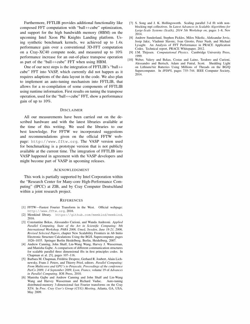
Figure 9 illustrates the performance of FFTLIB’s ball↔cube FFT using the FFTW back-end and without the lasttranspose operation. Across all the different grid geometries, itcan be noted that the ball↔cube approach achieves a higher

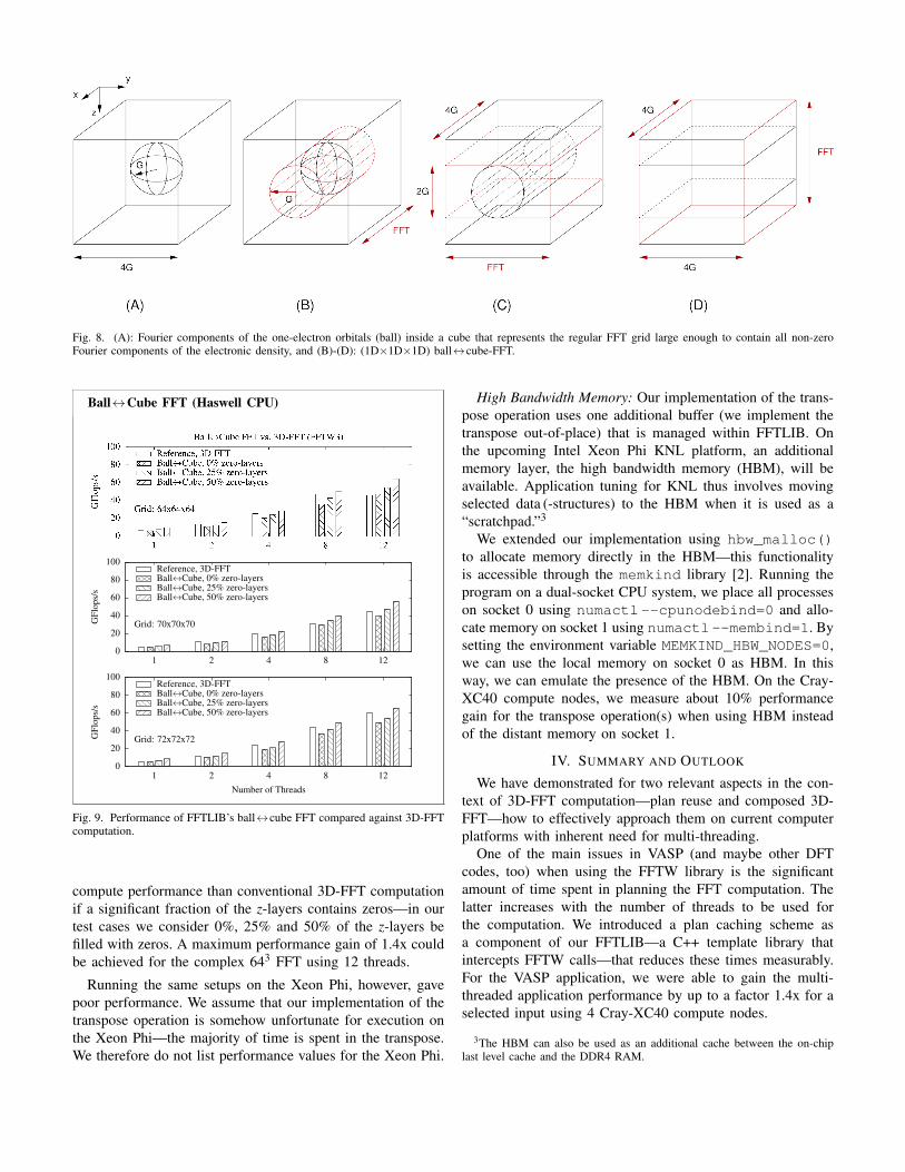
Fig. 8. (A): Fourier components of the one-electron orbitals (ball) inside a cube that represents the regular FFT grid large enough to contain all non-zeroFourier components of the electronic density, and (B)-(D): (1D×1D×1D) ball↔cube-FFT.

Ball↔Cube FFT (Haswell CPU)

0

20

40

60

80

100

1 2 4 8 12

GFl

ops/

s

Number of Threads

Ball↔Cube FFT vs. 3D-FFT (FFTW3)

Grid: 70x70x70

Reference, 3D-FFTBall↔Cube, 0% zero-layersBall↔Cube, 25% zero-layersBall↔Cube, 50% zero-layers

0

20

40

60

80

100

1 2 4 8 12

GFl

ops/

s

Number of Threads

Ball↔Cube FFT vs. 3D-FFT (FFTW3)

Grid: 72x72x72

Reference, 3D-FFTBall↔Cube, 0% zero-layersBall↔Cube, 25% zero-layersBall↔Cube, 50% zero-layers

Fig. 9. Performance of FFTLIB’s ball↔cube FFT compared against 3D-FFTcomputation.

compute performance than conventional 3D-FFT computationif a significant fraction of the z-layers contains zeros—in ourtest cases we consider 0%, 25% and 50% of the z-layers befilled with zeros. A maximum performance gain of 1.4x couldbe achieved for the complex 643 FFT using 12 threads.

Running the same setups on the Xeon Phi, however, gavepoor performance. We assume that our implementation of thetranspose operation is somehow unfortunate for execution onthe Xeon Phi—the majority of time is spent in the transpose.We therefore do not list performance values for the Xeon Phi.

High Bandwidth Memory: Our implementation of the trans-pose operation uses one additional buffer (we implement thetranspose out-of-place) that is managed within FFTLIB. Onthe upcoming Intel Xeon Phi KNL platform, an additionalmemory layer, the high bandwidth memory (HBM), will beavailable. Application tuning for KNL thus involves movingselected data (-structures) to the HBM when it is used as a“scratchpad.”3

We extended our implementation using hbw_malloc()to allocate memory directly in the HBM—this functionalityis accessible through the memkind library [2]. Running theprogram on a dual-socket CPU system, we place all processeson socket 0 using numactl--cpunodebind=0 and allo-cate memory on socket 1 using numactl--membind=1. Bysetting the environment variable MEMKIND_HBW_NODES=0,we can use the local memory on socket 0 as HBM. In thisway, we can emulate the presence of the HBM. On the Cray-XC40 compute nodes, we measure about 10% performancegain for the transpose operation(s) when using HBM insteadof the distant memory on socket 1.

IV. SUMMARY AND OUTLOOK

We have demonstrated for two relevant aspects in the con-text of 3D-FFT computation—plan reuse and composed 3D-FFT—how to effectively approach them on current computerplatforms with inherent need for multi-threading.

One of the main issues in VASP (and maybe other DFTcodes, too) when using the FFTW library is the significantamount of time spent in planning the FFT computation. Thelatter increases with the number of threads to be used forthe computation. We introduced a plan caching scheme asa component of our FFTLIB—a C++ template library thatintercepts FFTW calls—that reduces these times measurably.For the VASP application, we were able to gain the multi-threaded application performance by up to a factor 1.4x for aselected input using 4 Cray-XC40 compute nodes.

3The HBM can also be used as an additional cache between the on-chiplast level cache and the DDR4 RAM.

Furthermore, FFTLIB provides additional functionality likecomposed FFT computation with “ball↔cube” optimization,and support for the high bandwidth memory (HBM) on theupcoming Intel Xeon Phi Knights Landing platform. Us-ing synthetic benchmark kernels, we achieved up to 1.4xperformance gain over a conventional 3D-FFT computationon a Cray-XC40 compute node, and measured up to 10%performance increase for an out-of-place transpose operationas part of the “ball↔cube” FFT when using HBM.

One of our next steps is the integration of FFTLIB’s “ball↔cube” FFT into VASP, which currently did not happen as itrequires adaptions of the data layout in the code. We also planto implement an auto-tuning mechanism into FFTLIB, thatallows for a re-compilation of some components of FFTLIBusing runtime information. First results on tuning the transposeoperation, used for the “ball↔cube” FFT, show a performancegain of up to 10%.

DISCLAIMER

All our measurements have been carried out on the de-scribed hardware and with the latest libraries available atthe time of this writing. We used the libraries to ourbest knowledge. For FFTW we incorporated suggestionsand recommendations given on the official FFTW web-page: http://www.fftw.org. The VASP version usedfor benchmarking is a prototype version that is not publiclyavailable at the current time. The integration of FFTLIB intoVASP happened in agreement with the VASP developers andmight become part of VASP in upcoming releases.

ACKNOWLEDGMENT

This work is partially supported by Intel Corporation withinthe “Research Center for Many-core High-Performance Com-puting” (IPCC) at ZIB, and by Cray Computer Deutschlandwithin a joint research project.

REFERENCES

[1] FFTW—Fastest Fourier Transform in the West. Official webpage:http://www.fftw.org, 2016.

[2] Memkind library. https://github.com/memkind/memkind,2016.

[3] Constantine Bekas, Alessandro Curioni, and Wanda Andreoni. AppliedParallel Computing. State of the Art in Scientific Computing: 8thInternational Workshop, PARA 2006, Umea, Sweden, June 18-21, 2006,Revised Selected Papers, chapter New Scalability Frontiers in Ab InitioElectronic Structure Calculations Using the BG/L Supercomputer, pages1026–1035. Springer Berlin Heidelberg, Berlin, Heidelberg, 2007.

[4] Andrew Canning, John Shalf, Lin-Wang Wang, Harvey J. Wasserman,and Manisha Gajbe. A comparison of different communication structuresfor scalable parallel three dimensional ffts in first principles codes. InChapman et al. [5], pages 107–116.

[5] Barbara M. Chapman, Frederic Desprez, Gerhard R. Joubert, Alain Lich-newsky, Frans J. Peters, and Thierry Priol, editors. Parallel Computing:From Multicores and GPU’s to Petascale, Proceedings of the conferenceParCo 2009, 1-4 September 2009, Lyon, France, volume 19 of Advancesin Parallel Computing. IOS Press, 2010.

[6] Manisha Gajbe and Andrew Canning and John Shalf and Lin-WangWang and Harvey Wasserman and Richard Vuduc. Auto-tuningdistributed-memory 3-dimensional fast Fourier transforms on the CrayXT4. In Proc. Cray User’s Group (CUG) Meeting, Atlanta, GA, USA,May 2009.

[7] S. Song and J. K. Hollingsworth. Scaling parallel 3-d fft with non-blocking mpi collectives. In Latest Advances in Scalable Algorithms forLarge-Scale Systems (ScalA), 2014 5th Workshop on, pages 1–8, Nov2014.

[8] Andrew Sunderland, Stephen Pickles, Milos Nikolic, Aleksandar Jovic,Josip Jakic, Vladimir Slavnic, Ivan Girotto, Peter Nash, and MichaelLysaght. An Analysis of FFT Performance in PRACE ApplicationCodes. Technical report, PRACE Whitepaper, 2012.

[9] J.M. Thijssen. Computational Physics. Cambridge University Press,1999.

[10] Weber, Valery and Bekas, Costas and Laino, Teodoro and Curioni,Alessandro and Bertsch, Adam and Futral, Scott. Shedding Lighton Lithium/Air Batteries Using Millions of Threads on the BG/QSupercomputer. In IPDPS, pages 735–744. IEEE Computer Society,2014.