J Math Imaging Vis (2012) 42:163–175DOI 10.1007/s10851-011-0276-0

On Endmember Identification in Hyperspectral ImagesWithout Pure Pixels: A Comparison of Algorithms

Javier Plaza · Eligius M.T. Hendrix ·Inmaculada García · Gabriel Martín · Antonio Plaza

Published online: 25 March 2011© Springer Science+Business Media, LLC 2011

Abstract Hyperspectral imaging is an active area of re-search in Earth and planetary observation. One of the mostimportant techniques for analyzing hyperspectral images isspectral unmixing, in which mixed pixels (resulting from in-sufficient spatial resolution of the imaging sensor) are de-composed into a collection of spectrally pure constituentspectra, called endmembers weighted by their correspondentfractions, or abundances. Over the last years, several algo-rithms have been developed for automatic endmember ex-traction. Many of them assume that the images contain atleast one pure spectral signature for each distinct material.However, this assumption is usually not valid due to spa-tial resolution, mixing phenomena, and other considerations.A recent trend in the hyperspectral imaging community is todesign endmember identification algorithms which do notassume the presence of pure pixels. Despite the prolifera-tion of this kind of algorithms, many of which are based onminimum enclosing simplex concepts, a rigorous quantita-

J. Plaza (�) · G. Martín · A. PlazaHyperspectral Computing Laboratory, Dept. Technology ofComputers and Communications, University of Extremadura,Avda. de la Universidad s/n, 10071 Caceres, Spaine-mail: jplaza@unex.es

G. Martíne-mail: gamahefpi@unex.es

A. Plazae-mail: aplaza@unex.es

E.M.T. Hendrix · I. GarcíaDepartment of Computer Architecture, University of Málaga,29071 Málaga, Spain

E.M.T. Hendrixe-mail: Eligius.Hendrix@wur.nl

I. Garcíae-mail: igarcia@ual.es

tive and comparative assessment is not yet available. In thispaper, we provide a comparative analysis of endmember ex-traction algorithms without the pure pixel assumption. In ourexperiments we use synthetic hyperspectral data sets (con-structed using fractals) and real hyperspectral scenes col-lected by NASA’s Jet Propulsion Laboratory.

Keywords Hyperspectral imaging · Endmemberextraction · Spectral unmixing · Minimum enclosingsimplex

1 Introduction

Hyperspectral imaging has been transformed from a sparseresearch tool into a commodity product available to a broaduser community [1]. The wealth of spectral informationavailable from advanced hyperspectral imaging instrumentscurrently in operation has opened new perspectives in manyapplication domains, such as monitoring of environmen-tal and urban processes or risk prevention and response,including—among others—tracking wildfires, detecting bi-ological threats, and monitoring oil spills and other typesof chemical contamination. Advanced hyperspectral instru-ments such as NASA’s Airborne Visible Infra-Red ImagingSpectrometer (AVIRIS) [2] are now able to cover the wave-length region from 0.4 to 2.5 μm using more than 200 spec-tral channels, at nominal spectral resolution of 10 nm.

In hyperspectral imaging, endmember extraction is theprocess of selecting a collection of pure signature spectraof the materials present in a remotely sensed hyperspectralscene. These pure signatures are then used to decompose thescene into a set of so-called abundance fractions by meansof a spectral unmixing algorithm. Most techniques available

164 J Math Imaging Vis (2012) 42:163–175

in endmember extraction literature have been designed un-der the pure pixel assumption, i.e., they assume that the in-put hyperspectral data set contains at least one pure observa-tion for each distinct material present in the collected scene,and therefore a search procedure aimed at finding the mostspectrally pure signatures in the input scene is correct [3].Techniques include, among many others [4], the orthogonalsubspace projection (OSP) algorithm [5], the N-FINDR al-gorithm [6], a vertex component analysis (VCA) [7], the it-erative error analysis (IEA) [8], and other approaches basedon mathematical morphology [9] and lattice auto-associativememories [10, 11]. Maximum volume techniques, of whichN-FINDR is a representative algorithm, have found wide ac-ceptance in the community [12]. This technique looks forthe set of pixels filling the largest possible volume by inflat-ing a simplex inside the data.

Although the procedure adopted by N-FINDR has beenquite successful when pure pixels are present in the originalhyperspectral image, given the spatial resolution of state-of-the-art imaging spectrometers and the presence of the mix-ture phenomenon at different scales (even at microscopiclevels), this assumption is not true for many nowadays im-ages where pixels are completely mixed [13]. In order todeal with this important issue, other methods have been de-veloped that do not assume the presence of pure signaturesin the input data. Instead, these methods aim at generatingvirtual endmembers (not necessarily present in the set com-prised by input data samples). Techniques in this categoryinclude volume minimization approaches inspired by theseminal minimum volume transform (MVT) algorithm [14],such as the minimum volume constrained non-negative ma-trix factorization method (MVC-NMF) [15], the minimumvolume simplex analysis (MVSA) algorithm [16], the con-vex analysis-based minimum volume enclosing simplex al-gorithm (MVES) [17], the simplex identification via splitaugmented Lagrangian (SISAL) algorithm [18], or the iter-ative constrained endmembers (ICE) [19].

Despite the proliferation of endmember identification al-gorithms designed outside the pure pixel stream, availablealgorithms have not been rigorously compared by using aunified scheme. In this paper, we present a comparativestudy of endmember selection algorithms without the purepixel assumption, using both simulated and real hyperspec-tral data sets. The major contributions of this work are:(1) the development of a framework and test set for ex-perimental comparison of endmember selection algorithmswithout the pure pixel assumption, and (2) an assessment ofthe state of the art for endmember identification by drawingcomparisons between substantially different approaches tothe problem in rigorous fashion. The comparison includesalgorithms with and without the pure pixel assumption, in away that each method is fairly compared with others on thesame common ground. The investigation in this paper fol-lows the path initiated in [3], but substantially expands the

study by considering algorithms proposed in recent yearsand which present significant innovations with regards tomethods designed under the pure pixel assumption. The lat-ter category of algorithms may not be appropriate for an-alyzing data sets provided by the new generation of hy-perspectral imaging instruments, which continue increasingtheir spectral resolution at the expense of maintaining (oreven decreasing) the spatial resolution in the hope of imag-ing larger portions of the surface of the Earth.

The remainder of the paper is structured as follows. Sec-tion 2 describes the algorithms that will be compared in thisstudy. Section 3 presents the comparative framework, per-formance criteria and test set, which comprises a databaseof simulated data sets (which have been generated in thiswork using fractals) and a real AVIRIS hyperspectral im-age. In Sect. 4, a comparative performance analysis for thealgorithms described in Sect. 2 is presented and discussed.Finally, Sect. 5 points out main concluding statements de-rived from this paper and future research opportunities.

2 Endmember Identification Algorithms

In this section, we describe several endmember identifica-tion algorithms designed under the linear mixture model as-sumption. Let us denote the reflectance at channel i from agiven pixel of the original hyperspectral image as follows:

yi =p∑

j=1

ρijαj + wi, (1)

where ρij denotes the reflectance of endmember j at wave-length λi , αj denotes the abundance of endmember j at theconsidered pixel, and p is the number of endmembers. Theabundances are generally subject to the abundance sum-to-one constraint (ASC) and the abundance non-negativity con-straint (ANC):

p∑

j=1

αj = 1, αj ≥ 0, j = 1, . . . , p. (2)

Let yi be an B × 1 vector, where B is the total number ofbands, and mj ≡ [ρ1j , ρ2j , . . . , ρBj ]T be the spectral sig-nature of the j th endmember. Expression (1) can then bewritten in compact matrix form as:

Y = MS + W, (3)

where Y is a hyperspectral image made up of n pixel vec-tors in total, defined as Y ≡ [y1, . . . ,yn] ∈ R

B×n. M ≡[m1,m2, . . . ,mp] ∈ R

B×p is a matrix containing the sig-natures of the endmembers present in the pixel. S ≡[α1, . . . ,αn] ∈ R

p×n is a matrix containing the fractionalabundances, and W ∈ R

B×n models additive noise. Several

J Math Imaging Vis (2012) 42:163–175 165

techniques have been adopted in the literature to estimatethe matrix of endmembers M by assuming the presence orabsence of pure pixels in the original hyperspectral data. Inthe following, we describe the most relevant approaches ineach category.

2.1 Techniques Designed Under the Pure Pixel Assumption

These algorithms assume the presence in the original hy-perspectral image of at least one pure pixel per endmember,meaning that there is at least one pixel containing mj foreach endmember j being a vertex of the simplex encom-passed by the data. Although this assumption enables thedesign of efficient algorithms from a computational point ofview, it also imposes a requisite that may not hold in mostreal analysis scenarios.

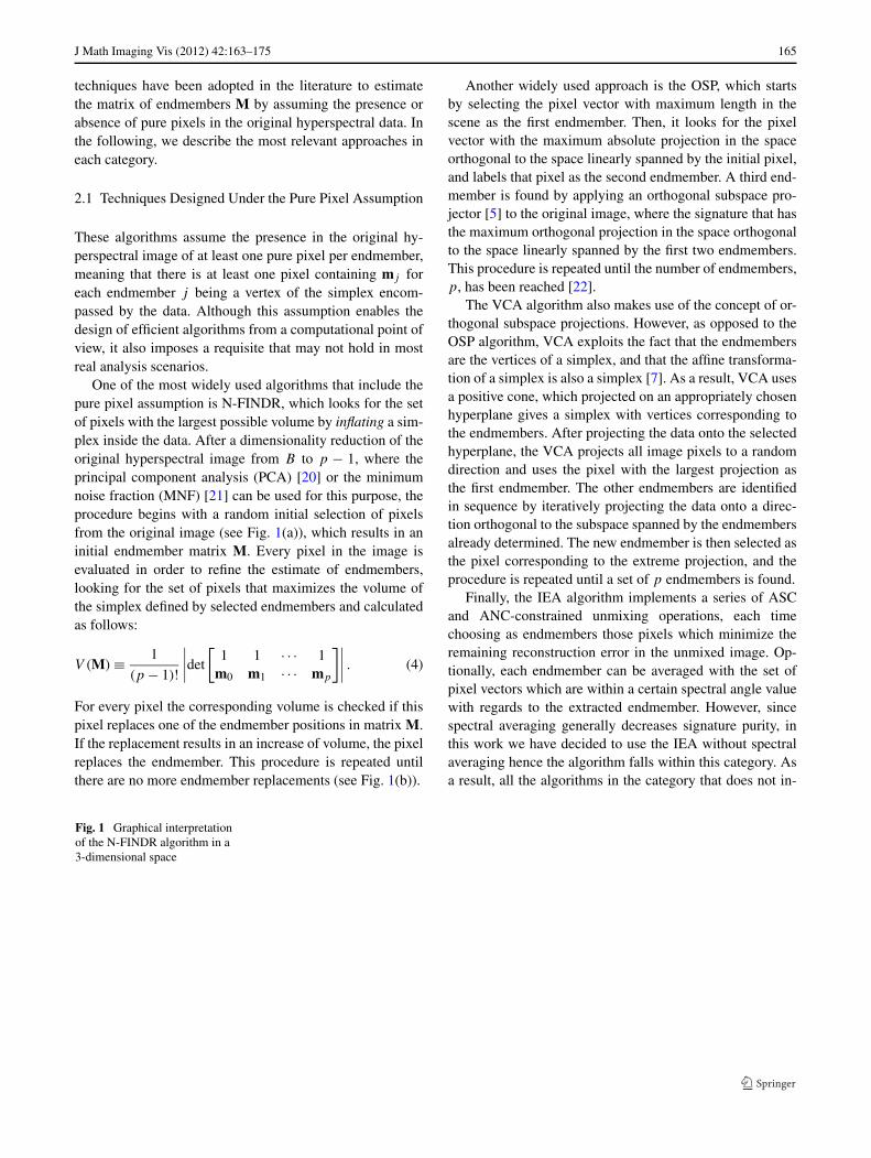
One of the most widely used algorithms that include thepure pixel assumption is N-FINDR, which looks for the setof pixels with the largest possible volume by inflating a sim-plex inside the data. After a dimensionality reduction of theoriginal hyperspectral image from B to p − 1, where theprincipal component analysis (PCA) [20] or the minimumnoise fraction (MNF) [21] can be used for this purpose, theprocedure begins with a random initial selection of pixelsfrom the original image (see Fig. 1(a)), which results in aninitial endmember matrix M. Every pixel in the image isevaluated in order to refine the estimate of endmembers,looking for the set of pixels that maximizes the volume ofthe simplex defined by selected endmembers and calculatedas follows:

V (M) ≡ 1

(p − 1)!∣∣∣∣det

[1 1 · · · 1

m0 m1 · · · mp

]∣∣∣∣ . (4)

For every pixel the corresponding volume is checked if thispixel replaces one of the endmember positions in matrix M.If the replacement results in an increase of volume, the pixelreplaces the endmember. This procedure is repeated untilthere are no more endmember replacements (see Fig. 1(b)).

Another widely used approach is the OSP, which startsby selecting the pixel vector with maximum length in thescene as the first endmember. Then, it looks for the pixelvector with the maximum absolute projection in the spaceorthogonal to the space linearly spanned by the initial pixel,and labels that pixel as the second endmember. A third end-member is found by applying an orthogonal subspace pro-jector [5] to the original image, where the signature that hasthe maximum orthogonal projection in the space orthogonalto the space linearly spanned by the first two endmembers.This procedure is repeated until the number of endmembers,p, has been reached [22].

The VCA algorithm also makes use of the concept of or-thogonal subspace projections. However, as opposed to theOSP algorithm, VCA exploits the fact that the endmembersare the vertices of a simplex, and that the affine transforma-tion of a simplex is also a simplex [7]. As a result, VCA usesa positive cone, which projected on an appropriately chosenhyperplane gives a simplex with vertices corresponding tothe endmembers. After projecting the data onto the selectedhyperplane, the VCA projects all image pixels to a randomdirection and uses the pixel with the largest projection asthe first endmember. The other endmembers are identifiedin sequence by iteratively projecting the data onto a direc-tion orthogonal to the subspace spanned by the endmembersalready determined. The new endmember is then selected asthe pixel corresponding to the extreme projection, and theprocedure is repeated until a set of p endmembers is found.

Finally, the IEA algorithm implements a series of ASCand ANC-constrained unmixing operations, each timechoosing as endmembers those pixels which minimize theremaining reconstruction error in the unmixed image. Op-tionally, each endmember can be averaged with the set ofpixel vectors which are within a certain spectral angle valuewith regards to the extracted endmember. However, sincespectral averaging generally decreases signature purity, inthis work we have decided to use the IEA without spectralaveraging hence the algorithm falls within this category. Asa result, all the algorithms in the category that does not in-

Fig. 1 Graphical interpretationof the N-FINDR algorithm in a3-dimensional space

166 J Math Imaging Vis (2012) 42:163–175

clude the pure pixel assumption (described below) are basedon minimum enclosing volume concepts.

2.2 Techniques Designed Without the Pure PixelAssumption

Most of the techniques in this category adopt a minimumvolume strategy aimed at finding the endmember matrix Mby minimizing the volume of the simplex defined by itscolumns and containing the endmembers. This is a non-convex optimization problem much harder than those con-sidered in the previous subsection in which the endmembersare assumed to belong to the input hyperspectral image.

Craig’s seminal work established the concepts regard-ing the algorithms of minimum volume type. The MVSAand SISAL algorithms implement a robust version of theminimum volume concept. The robustness is introducedby allowing the ANC to be violated. These violations areweighted using a soft constraint given by the hinge lossfunction (hinge(x) = 0 if x ≥ 0 and −x if x < 0). Afterreducing the dimensionality of the input data from B top−1, MVSA/SISAL aim at solving the following optimiza-tion problem:

Q = arg maxQ

log(|det(Q)|) − λ1Tp hinge(QY)1n (5)

s.t.: 1Tp Q = qm, (6)

where Q ≡ M−1, 1p and 1n are column vectors of ones ofsizes p and n (n stands for the number of spectral vectors),respectively, qm ≡ 1T

p Y−1p with Yp being any set of linearly

independent spectral vectors taken from the hyperspectraldata set Y, and λ is a regularization parameter. Here, maxi-mizing log(|det(Q)|) is equivalent to minimizing V (M).

The MVES algorithm aims at solving the optimizationproblem (5) with λ = ∞, i.e., for hard ANC but without us-ing a de-noising strategy prior to the data analysis. Instead,MVES implements a cyclic minimization using linear pro-gramming. Although the optimization problem (5) is non-convex, it is proved in [17] that the existence of pure pixelsis a sufficient condition for MVES to perfectly identify thetrue endmembers.

The MVC-NMF algorithm solves the following opti-mization problem applied to the original data set, i.e., with-out dimensionality reduction, as follows:

M = arg minM∈RB×p

1

2‖Y − MS‖2

F + λV 2(M)

s.t.: = M ≥ 0, S ≥ 0, 1T S = 1Tn ,

(7)

where ‖A‖2F ≡ tr(AT A) is the Frobenius norm of matrix A

and λ is a regularization parameter. The optimization (7)minimizes a two term objective function, where the term

(1/2)‖Y − MS‖2F measures the approximation error and

the term V 2(M) measures the square of the volume of thesimplex defined by the columns of M. The regularizationparameter λ controls the tradeoff between the reconstruc-tion errors and simplex volumes. MVC-NMF implementsa sequence of alternate minimizations with respect to S(quadratic programming problem) and with respect to M(non-convex programming problem). The major differencebetween MVC-NMF and MVSA/SISAL algorithms is thatthe latter allows violations of the ANC, whereas the formerdoes not.

Finally, we have recently developed a new minimum vol-ume enclosing algorithm called MINVEST [23]. This algo-rithm adopts a hierarchical vision of the spectral unmixingproblem. First, it uses PCA to reduce the dimensionality ofthe data from B to p − 1. Then, it minimizes the volume ofan enclosing simplex in the reduced space while estimatingthe fractional abundance of vertices in simultaneous fash-ion. Although the concept of MINVEST is similar to that ofother algorithms discussed in this section, a distinguishingfeature is that MINVEST takes care of noise by iterativelyidentifying and removing pixels that fall outside the simplexto be estimated.

2.3 Illustrative Example Without Pure Pixels

To conclude this section, we illustrate via a simple toy exam-ple the potential advantages of algorithms without the purepixel assumption. For this purpose, we have generated a toydata set made up of linear mixtures of three endmembers(designated as ‘A’, ‘B’ and ‘C’, respectively) where the max-imum degree of purity of any of the considered endmembersin the available observations is given a maximum of 70% ofan endmember. The endmembers have been randomly se-lected from a library of mineral spectral available onlinefrom U.S. Geological Survey (USGS). The simulated dataset does not include any pure observations. A peculiarity ofthis situation is that, although the pure signatures ‘A’, ‘B’and ‘C’ have been used to create all the simulated mixtures,the pure observations themselves (which can be consideredas ground-truth) are not included in the input data to be pro-cessed. As a result, finding p = 3 endmembers in this toy ex-ample is a challenging problem. In this case, algorithms withthe pure pixel assumption (e.g., N-FINDR) tackle the prob-lem by finding the best combination that can be formed us-ing samples contained in the data set. Quite opposite, mini-mum enclosing-based approaches (e.g., MINVEST) addressthe problem by finding the simplex with minimum volumethat can enclose all the observations. The situation is graph-ically illustrated in Fig. 2, which plots the outcome of theendmember identification process by N-FINDR and MIN-VEST in a two-dimensional space given by the first twoPCA components. As shown in Fig. 2, only MINVEST can

J Math Imaging Vis (2012) 42:163–175 167

Fig. 2 (Color online) (a) Two-dimensional representation of a toy data set without pure samples, and endmembers extracted by MINVEST (red)and N-FINDR (green). (b) Coordinates of the endmembers and simplices defined by the endmembers extracted by MINVEST (red) and N-FINDR(green)

Fig. 3 Synthetic images, where spatial patterns were generated using fractals (left) then segmented into clusters (right)

successfully retrieve the endmembers (even if these are notcontained in the input data).

3 Framework, Test Set and Criteria

3.1 Synthetic Hyperspectral Data

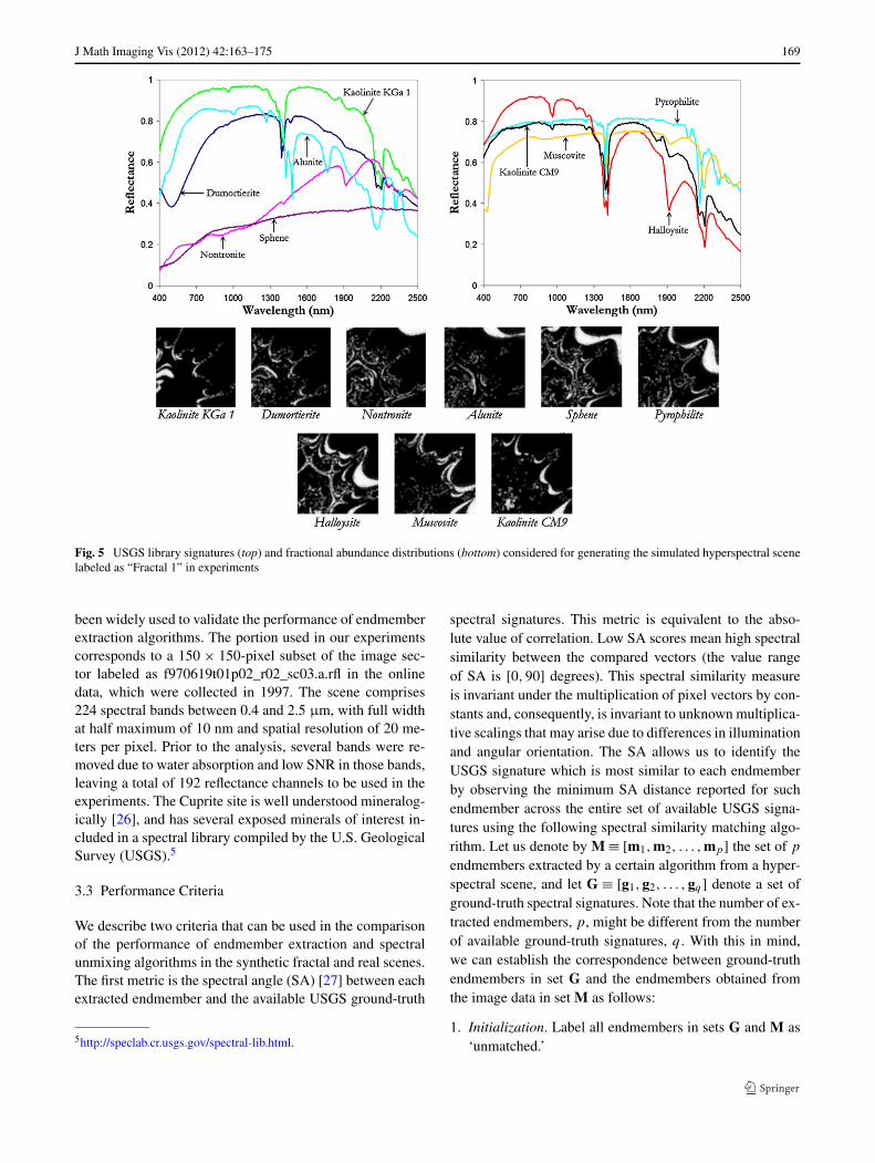
A database of five 100 × 100-pixel synthetic hyperspectralscenes has been created using fractals to generate distinctspatial patterns, which are then used to simulate linear mix-tures of a set of endmember signatures randomly selectedfrom a spectral library compiled by the U.S. Geological Sur-vey (USGS)1 and made up of a total of 420 spectral signa-tures. The leftmost part of Fig. 3 displays the five fractalimages used in the simulations. These images are furtherdivided into a number of clusters using the k-means algo-rithm in [24], where the number of clusters extracted from

1http://speclab.cr.usgs.gov/spectral-lib.html.

the five fractal images was always larger than the number ofendmember signatures, fixed in our experiments to p = 9.The resulting clusters are displayed in the rightmost part ofFig. 3. A crucial step in the simulation procedure is how toassign a spectral signature to each cluster. For this purpose,we have implemented an automatic procedure that follows asimple strategy in which the p = 9 signatures are first as-signed to spatially disjoint regions belonging to differentclusters. The remaining regions are then assigned spectralsignatures in an automatic way, ensuring that: (1) spatiallyadjacent clusters always have different signatures associatedto them, and (2) there is a balance among the overall num-ber of pixels in the image which are associated to each spec-tral signature. Inside each region, the abundance proportionsof spectral signatures have been generated following a pro-cedure that tries to imitate reality as much as possible, i.e.those pixels closer to the borders of the regions are moreheavily mixed, while the pixels located at the center of theregions are more spectrally pure in nature. This is accom-plished by linearly mixing the signature associated to eachcluster with those associated to neighboring clusters, mak-

168 J Math Imaging Vis (2012) 42:163–175

Fig. 4 Block diagramdescribing our procedure forgenerating synthetichyperspectral images

ing sure that the most spectrally pure signature remains atthe center of the region while signature purity decreases lin-early away from the center to the borders of the regions. Forthis purpose, a Gaussian filter is applied where the width ofthe Gaussian is carefully adjusted according to the width ofeach window. With the aforementioned procedure, which isgraphically illustrated by a block diagram in Fig. 4, the sim-ulated regions exhibit the following properties:

1. All the simulated pixels inside a region are mixed, andthe simulated image does not contain completely purepixels. This increases the complexity of the unmixingproblem and simulates the situation often encountered inreal-world analysis scenarios, in which completely purepixels are rarely found.

2. Pixels close to the borders of the region are more heavilymixed than those in the center of the region.

3. If the simulated region is sufficiently large, the pixels lo-cated at the center can exhibit a degree of purity of 99%of a certain endmember. However, if the size of the simu-lated region is small, the degree of purity of pixels at thecenter of the region can decrease until 95% of a certainendmember, while pixels located in the region bordersare generally more heavily mixed.

To conclude the simulation process, zero-mean Gaussiannoise was added to the scenes in different signal to noiseratios (SNRs)—from 30 to 110—to simulate contributionsfrom ambient and instrumental sources, following the proce-dure described in [5]. For illustrative purposes, Fig. 5 shows

the spectra of the USGS signatures used in the simulation ofone of the synthetic scenes (the one labeled as “Fractal 1”in Fig. 3). The full database of simulated hyperspectral im-ages is available online.2 The abundance maps associated toeach reference USGS signature in the construction of thesynthetic scene are also displayed in Fig. 5, where blackcolor indicates 0% abundance of the corresponding mineral,white color indicates 100% abundance of the mineral, andthe fractional abundances in each pixel of the scene sum tounity, thus ensuring that the simulated fractal images strictlyadhere to a fully constrained linear mixture model.

Finally, we emphasize that other methods exist for perfor-mance evaluation of endmember extraction and hyperspec-tral imaging algorithms using synthetic hyperspectral im-ages. Of particular relevance is a Matlab toolbox (availableonline3) for generating synthetic endmember abundancesusing random fields and Legendre polynomials [25].

3.2 Real Hyperspectral Data

The real hyperspectral data set used in our experiments is thewell-known AVIRIS Cuprite data set, available online in re-flectance units4 after atmospheric correction. This scene has

2http://www.umbc.edu/rssipl/people/aplaza/fractals.zip.3http://www.ehu.es/ccwintco/index.php/Hyperspectral_Imagery_Synthesis_tools_for_MATLAB.4http://aviris.jpl.nasa.gov/html/aviris.freedata.html.

J Math Imaging Vis (2012) 42:163–175 169

Fig. 5 USGS library signatures (top) and fractional abundance distributions (bottom) considered for generating the simulated hyperspectral scenelabeled as “Fractal 1” in experiments

been widely used to validate the performance of endmemberextraction algorithms. The portion used in our experimentscorresponds to a 150 × 150-pixel subset of the image sec-tor labeled as f970619t01p02_r02_sc03.a.rfl in the onlinedata, which were collected in 1997. The scene comprises224 spectral bands between 0.4 and 2.5 μm, with full widthat half maximum of 10 nm and spatial resolution of 20 me-ters per pixel. Prior to the analysis, several bands were re-moved due to water absorption and low SNR in those bands,leaving a total of 192 reflectance channels to be used in theexperiments. The Cuprite site is well understood mineralog-ically [26], and has several exposed minerals of interest in-cluded in a spectral library compiled by the U.S. GeologicalSurvey (USGS).5

3.3 Performance Criteria

We describe two criteria that can be used in the comparisonof the performance of endmember extraction and spectralunmixing algorithms in the synthetic fractal and real scenes.The first metric is the spectral angle (SA) [27] between eachextracted endmember and the available USGS ground-truth

5http://speclab.cr.usgs.gov/spectral-lib.html.

spectral signatures. This metric is equivalent to the abso-lute value of correlation. Low SA scores mean high spectralsimilarity between the compared vectors (the value rangeof SA is [0,90] degrees). This spectral similarity measureis invariant under the multiplication of pixel vectors by con-stants and, consequently, is invariant to unknown multiplica-tive scalings that may arise due to differences in illuminationand angular orientation. The SA allows us to identify theUSGS signature which is most similar to each endmemberby observing the minimum SA distance reported for suchendmember across the entire set of available USGS signa-tures using the following spectral similarity matching algo-rithm. Let us denote by M ≡ [m1,m2, . . . ,mp] the set of p

endmembers extracted by a certain algorithm from a hyper-spectral scene, and let G ≡ [g1,g2, . . . ,gq ] denote a set ofground-truth spectral signatures. Note that the number of ex-tracted endmembers, p, might be different from the numberof available ground-truth signatures, q . With this in mind,we can establish the correspondence between ground-truthendmembers in set G and the endmembers obtained fromthe image data in set M as follows:

1. Initialization. Label all endmembers in sets G and M as‘unmatched.’

170 J Math Imaging Vis (2012) 42:163–175

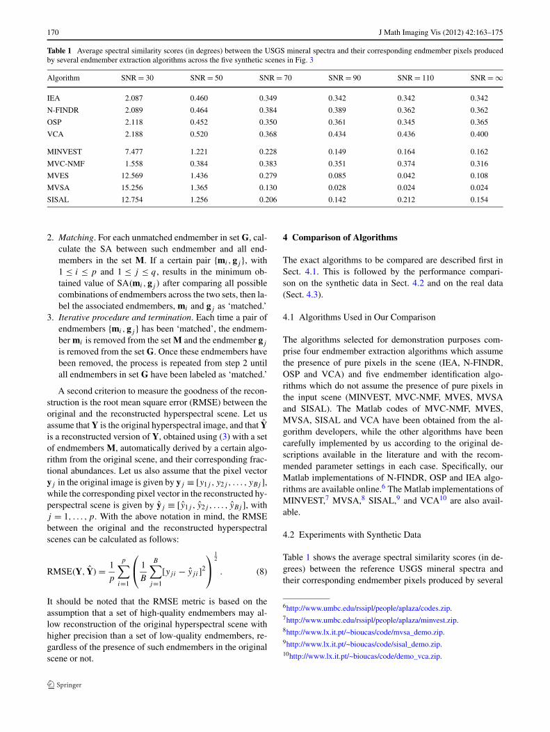
Table 1 Average spectral similarity scores (in degrees) between the USGS mineral spectra and their corresponding endmember pixels producedby several endmember extraction algorithms across the five synthetic scenes in Fig. 3

Algorithm SNR = 30 SNR = 50 SNR = 70 SNR = 90 SNR = 110 SNR = ∞

IEA 2.087 0.460 0.349 0.342 0.342 0.342

N-FINDR 2.089 0.464 0.384 0.389 0.362 0.362

OSP 2.118 0.452 0.350 0.361 0.345 0.365

VCA 2.188 0.520 0.368 0.434 0.436 0.400

MINVEST 7.477 1.221 0.228 0.149 0.164 0.162

MVC-NMF 1.558 0.384 0.383 0.351 0.374 0.316

MVES 12.569 1.436 0.279 0.085 0.042 0.108

MVSA 15.256 1.365 0.130 0.028 0.024 0.024

SISAL 12.754 1.256 0.206 0.142 0.212 0.154

2. Matching. For each unmatched endmember in set G, cal-culate the SA between such endmember and all end-members in the set M. If a certain pair {mi ,gj }, with1 ≤ i ≤ p and 1 ≤ j ≤ q , results in the minimum ob-tained value of SA(mi ,gj ) after comparing all possiblecombinations of endmembers across the two sets, then la-bel the associated endmembers, mi and gj as ‘matched.’

3. Iterative procedure and termination. Each time a pair ofendmembers {mi ,gj } has been ‘matched’, the endmem-ber mi is removed from the set M and the endmember gj

is removed from the set G. Once these endmembers havebeen removed, the process is repeated from step 2 untilall endmembers in set G have been labeled as ‘matched.’

A second criterion to measure the goodness of the recon-struction is the root mean square error (RMSE) between theoriginal and the reconstructed hyperspectral scene. Let usassume that Y is the original hyperspectral image, and that Yis a reconstructed version of Y, obtained using (3) with a setof endmembers M, automatically derived by a certain algo-rithm from the original scene, and their corresponding frac-tional abundances. Let us also assume that the pixel vectoryj in the original image is given by yj ≡ [y1j , y2j , . . . , yBj ],while the corresponding pixel vector in the reconstructed hy-perspectral scene is given by yj ≡ [y1j , y2j , . . . , yBj ], withj = 1, . . . , p. With the above notation in mind, the RMSEbetween the original and the reconstructed hyperspectralscenes can be calculated as follows:

RMSE(Y, Y) = 1

p

p∑

i=1

⎛

⎝ 1

B

B∑

j=1

[yji − yj i]2

⎞

⎠

12

. (8)

It should be noted that the RMSE metric is based on theassumption that a set of high-quality endmembers may al-low reconstruction of the original hyperspectral scene withhigher precision than a set of low-quality endmembers, re-gardless of the presence of such endmembers in the originalscene or not.

4 Comparison of Algorithms

The exact algorithms to be compared are described first inSect. 4.1. This is followed by the performance compari-son on the synthetic data in Sect. 4.2 and on the real data(Sect. 4.3).

4.1 Algorithms Used in Our Comparison

The algorithms selected for demonstration purposes com-prise four endmember extraction algorithms which assumethe presence of pure pixels in the scene (IEA, N-FINDR,OSP and VCA) and five endmember identification algo-rithms which do not assume the presence of pure pixels inthe input scene (MINVEST, MVC-NMF, MVES, MVSAand SISAL). The Matlab codes of MVC-NMF, MVES,MVSA, SISAL and VCA have been obtained from the al-gorithm developers, while the other algorithms have beencarefully implemented by us according to the original de-scriptions available in the literature and with the recom-mended parameter settings in each case. Specifically, ourMatlab implementations of N-FINDR, OSP and IEA algo-rithms are available online.6 The Matlab implementations ofMINVEST,7 MVSA,8 SISAL,9 and VCA10 are also avail-able.

4.2 Experiments with Synthetic Data

Table 1 shows the average spectral similarity scores (in de-grees) between the reference USGS mineral spectra andtheir corresponding endmember pixels produced by several

6http://www.umbc.edu/rssipl/people/aplaza/codes.zip.7http://www.umbc.edu/rssipl/people/aplaza/minvest.zip.8http://www.lx.it.pt/~bioucas/code/mvsa_demo.zip.9http://www.lx.it.pt/~bioucas/code/sisal_demo.zip.10http://www.lx.it.pt/~bioucas/code/demo_vca.zip.

J Math Imaging Vis (2012) 42:163–175 171

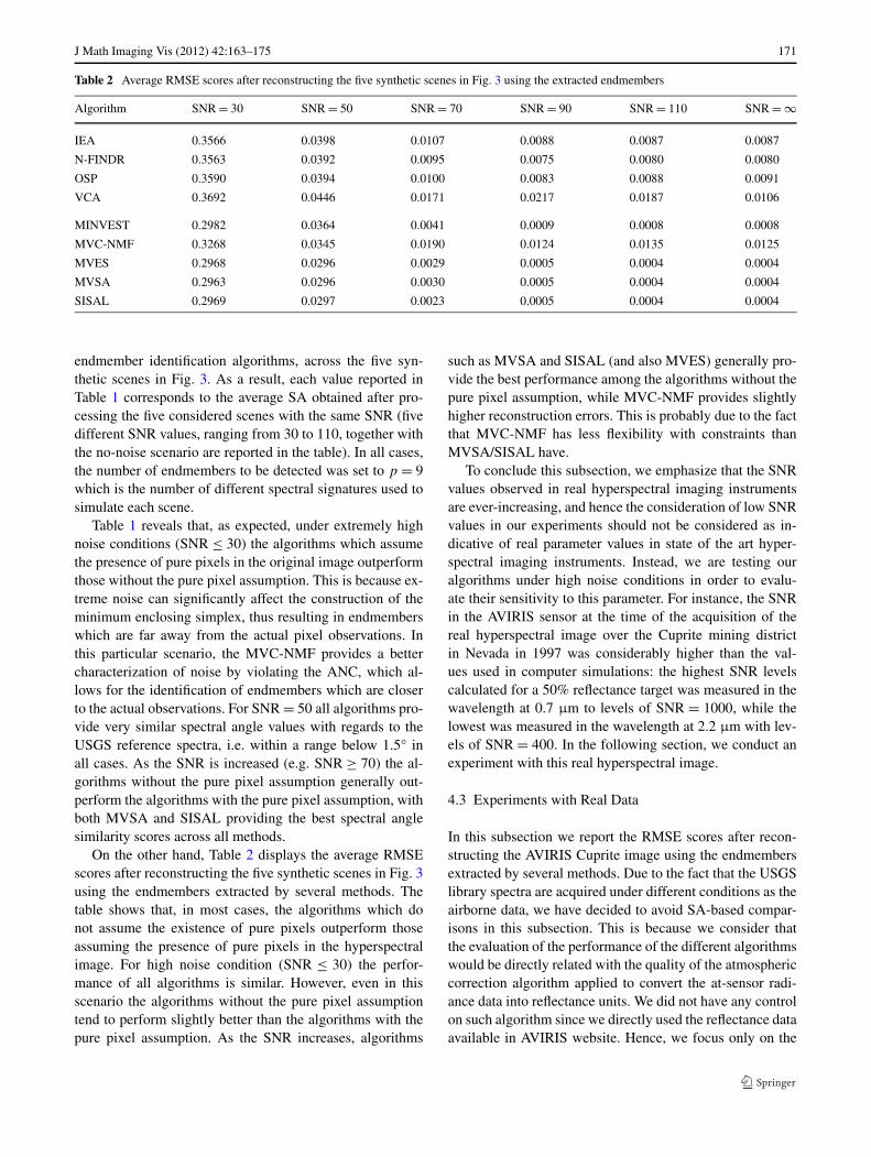
Table 2 Average RMSE scores after reconstructing the five synthetic scenes in Fig. 3 using the extracted endmembers

Algorithm SNR = 30 SNR = 50 SNR = 70 SNR = 90 SNR = 110 SNR = ∞

IEA 0.3566 0.0398 0.0107 0.0088 0.0087 0.0087

N-FINDR 0.3563 0.0392 0.0095 0.0075 0.0080 0.0080

OSP 0.3590 0.0394 0.0100 0.0083 0.0088 0.0091

VCA 0.3692 0.0446 0.0171 0.0217 0.0187 0.0106

MINVEST 0.2982 0.0364 0.0041 0.0009 0.0008 0.0008

MVC-NMF 0.3268 0.0345 0.0190 0.0124 0.0135 0.0125

MVES 0.2968 0.0296 0.0029 0.0005 0.0004 0.0004

MVSA 0.2963 0.0296 0.0030 0.0005 0.0004 0.0004

SISAL 0.2969 0.0297 0.0023 0.0005 0.0004 0.0004

endmember identification algorithms, across the five syn-thetic scenes in Fig. 3. As a result, each value reported inTable 1 corresponds to the average SA obtained after pro-cessing the five considered scenes with the same SNR (fivedifferent SNR values, ranging from 30 to 110, together withthe no-noise scenario are reported in the table). In all cases,the number of endmembers to be detected was set to p = 9which is the number of different spectral signatures used tosimulate each scene.

Table 1 reveals that, as expected, under extremely highnoise conditions (SNR ≤ 30) the algorithms which assumethe presence of pure pixels in the original image outperformthose without the pure pixel assumption. This is because ex-treme noise can significantly affect the construction of theminimum enclosing simplex, thus resulting in endmemberswhich are far away from the actual pixel observations. Inthis particular scenario, the MVC-NMF provides a bettercharacterization of noise by violating the ANC, which al-lows for the identification of endmembers which are closerto the actual observations. For SNR = 50 all algorithms pro-vide very similar spectral angle values with regards to theUSGS reference spectra, i.e. within a range below 1.5° inall cases. As the SNR is increased (e.g. SNR ≥ 70) the al-gorithms without the pure pixel assumption generally out-perform the algorithms with the pure pixel assumption, withboth MVSA and SISAL providing the best spectral anglesimilarity scores across all methods.

On the other hand, Table 2 displays the average RMSEscores after reconstructing the five synthetic scenes in Fig. 3using the endmembers extracted by several methods. Thetable shows that, in most cases, the algorithms which donot assume the existence of pure pixels outperform thoseassuming the presence of pure pixels in the hyperspectralimage. For high noise condition (SNR ≤ 30) the perfor-mance of all algorithms is similar. However, even in thisscenario the algorithms without the pure pixel assumptiontend to perform slightly better than the algorithms with thepure pixel assumption. As the SNR increases, algorithms

such as MVSA and SISAL (and also MVES) generally pro-vide the best performance among the algorithms without thepure pixel assumption, while MVC-NMF provides slightlyhigher reconstruction errors. This is probably due to the factthat MVC-NMF has less flexibility with constraints thanMVSA/SISAL have.

To conclude this subsection, we emphasize that the SNRvalues observed in real hyperspectral imaging instrumentsare ever-increasing, and hence the consideration of low SNRvalues in our experiments should not be considered as in-dicative of real parameter values in state of the art hyper-spectral imaging instruments. Instead, we are testing ouralgorithms under high noise conditions in order to evalu-ate their sensitivity to this parameter. For instance, the SNRin the AVIRIS sensor at the time of the acquisition of thereal hyperspectral image over the Cuprite mining districtin Nevada in 1997 was considerably higher than the val-ues used in computer simulations: the highest SNR levelscalculated for a 50% reflectance target was measured in thewavelength at 0.7 μm to levels of SNR = 1000, while thelowest was measured in the wavelength at 2.2 μm with lev-els of SNR = 400. In the following section, we conduct anexperiment with this real hyperspectral image.

4.3 Experiments with Real Data

In this subsection we report the RMSE scores after recon-structing the AVIRIS Cuprite image using the endmembersextracted by several methods. Due to the fact that the USGSlibrary spectra are acquired under different conditions as theairborne data, we have decided to avoid SA-based compar-isons in this subsection. This is because we consider thatthe evaluation of the performance of the different algorithmswould be directly related with the quality of the atmosphericcorrection algorithm applied to convert the at-sensor radi-ance data into reflectance units. We did not have any controlon such algorithm since we directly used the reflectance dataavailable in AVIRIS website. Hence, we focus only on the

172 J Math Imaging Vis (2012) 42:163–175

use of the RMSE metric. In all our experiments, the num-ber of endmembers to be identified was set to p = 9 af-ter the consensus reached between two of the most popu-lar methods for estimating the number of endmembers inhyperspectral data: HySime [28] and the VD concept [29],implemented using PF = 10−3 as the input false alarm prob-ability.

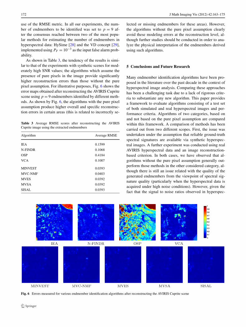
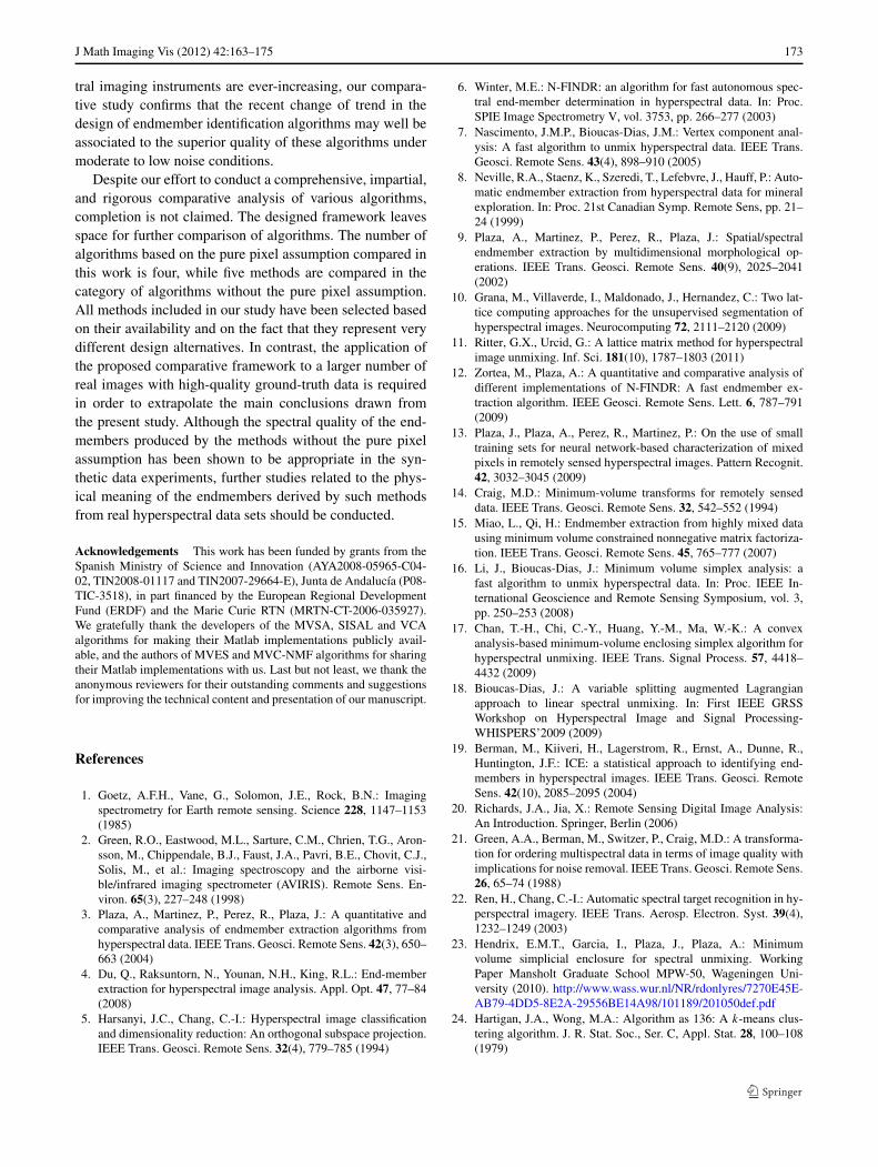
As shown in Table 3, the tendency of the results is simi-lar to that of the experiments with synthetic scenes for mod-erately high SNR values; the algorithms which assume thepresence of pure pixels in the image provide significantlyhigher reconstruction errors than those without the purepixel assumption. For illustrative purposes, Fig. 6 shows theerror maps obtained after reconstructing the AVIRIS Cupritescene using p = 9 endmembers identified by different meth-ods. As shown by Fig. 6, the algorithms with the pure pixelassumption produce higher overall and specific reconstruc-tion errors in certain areas (this is related to incorrectly se-

Table 3 Average RMSE scores after reconstructing the AVIRISCuprite image using the extracted endmembers

Algorithm Average RMSE

IEA 0.1599

N-FINDR 0.1068

OSP 0.4184

VCA 0.1007

MINVEST 0.0393

MVC-NMF 0.0403

MVES 0.0392

MVSA 0.0392

SISAL 0.0393

lected or missing endmembers for these areas). However,the algorithms without the pure pixel assumption clearlyavoid these modeling errors at the reconstruction level, al-though further studies should be conducted in order to ana-lyze the physical interpretation of the endmembers derivedusing such algorithms.

5 Conclusions and Future Research

Many endmember identification algorithms have been pro-posed in the literature over the past decade in the context ofhyperspectral image analysis. Comparing these approacheshas been a challenging task due to a lack of rigorous crite-ria to substantiate any new algorithm. This paper providesa framework to evaluate algorithms consisting of a test setof both simulated and real hyperspectral images and per-formance criteria. Algorithms of two categories, based onand not based on the pure pixel assumption are comparedwithin this framework. A comparison of methods has beencarried out from two different scopes. First, the issue wasundertaken under the assumption that reliable ground-truthspectral signatures are available via synthetic hyperspec-tral images. A further experiment was conducted using realAVIRIS hyperspectral data and an image reconstruction-based criterion. In both cases, we have observed that al-gorithms without the pure pixel assumption generally out-perform those methods in the other considered category, al-though there is still an issue related with the quality of thegenerated endmembers from the viewpoint of spectral sig-nature quality (particularly when the hyperspectral data isacquired under high noise conditions). However, given thefact that the signal to noise ratios observed in hyperspec-

Fig. 6 Errors measured for various endmember identification algorithms after reconstructing the AVIRIS Cuprite scene

J Math Imaging Vis (2012) 42:163–175 173

tral imaging instruments are ever-increasing, our compara-tive study confirms that the recent change of trend in thedesign of endmember identification algorithms may well beassociated to the superior quality of these algorithms undermoderate to low noise conditions.

Despite our effort to conduct a comprehensive, impartial,and rigorous comparative analysis of various algorithms,completion is not claimed. The designed framework leavesspace for further comparison of algorithms. The number ofalgorithms based on the pure pixel assumption compared inthis work is four, while five methods are compared in thecategory of algorithms without the pure pixel assumption.All methods included in our study have been selected basedon their availability and on the fact that they represent verydifferent design alternatives. In contrast, the application ofthe proposed comparative framework to a larger number ofreal images with high-quality ground-truth data is requiredin order to extrapolate the main conclusions drawn fromthe present study. Although the spectral quality of the end-members produced by the methods without the pure pixelassumption has been shown to be appropriate in the syn-thetic data experiments, further studies related to the phys-ical meaning of the endmembers derived by such methodsfrom real hyperspectral data sets should be conducted.

Acknowledgements This work has been funded by grants from theSpanish Ministry of Science and Innovation (AYA2008-05965-C04-02, TIN2008-01117 and TIN2007-29664-E), Junta de Andalucía (P08-TIC-3518), in part financed by the European Regional DevelopmentFund (ERDF) and the Marie Curie RTN (MRTN-CT-2006-035927).We gratefully thank the developers of the MVSA, SISAL and VCAalgorithms for making their Matlab implementations publicly avail-able, and the authors of MVES and MVC-NMF algorithms for sharingtheir Matlab implementations with us. Last but not least, we thank theanonymous reviewers for their outstanding comments and suggestionsfor improving the technical content and presentation of our manuscript.

References

1. Goetz, A.F.H., Vane, G., Solomon, J.E., Rock, B.N.: Imagingspectrometry for Earth remote sensing. Science 228, 1147–1153(1985)

2. Green, R.O., Eastwood, M.L., Sarture, C.M., Chrien, T.G., Aron-sson, M., Chippendale, B.J., Faust, J.A., Pavri, B.E., Chovit, C.J.,Solis, M., et al.: Imaging spectroscopy and the airborne visi-ble/infrared imaging spectrometer (AVIRIS). Remote Sens. En-viron. 65(3), 227–248 (1998)

3. Plaza, A., Martinez, P., Perez, R., Plaza, J.: A quantitative andcomparative analysis of endmember extraction algorithms fromhyperspectral data. IEEE Trans. Geosci. Remote Sens. 42(3), 650–663 (2004)

4. Du, Q., Raksuntorn, N., Younan, N.H., King, R.L.: End-memberextraction for hyperspectral image analysis. Appl. Opt. 47, 77–84(2008)

5. Harsanyi, J.C., Chang, C.-I.: Hyperspectral image classificationand dimensionality reduction: An orthogonal subspace projection.IEEE Trans. Geosci. Remote Sens. 32(4), 779–785 (1994)

6. Winter, M.E.: N-FINDR: an algorithm for fast autonomous spec-tral end-member determination in hyperspectral data. In: Proc.SPIE Image Spectrometry V, vol. 3753, pp. 266–277 (2003)

7. Nascimento, J.M.P., Bioucas-Dias, J.M.: Vertex component anal-ysis: A fast algorithm to unmix hyperspectral data. IEEE Trans.Geosci. Remote Sens. 43(4), 898–910 (2005)

8. Neville, R.A., Staenz, K., Szeredi, T., Lefebvre, J., Hauff, P.: Auto-matic endmember extraction from hyperspectral data for mineralexploration. In: Proc. 21st Canadian Symp. Remote Sens, pp. 21–24 (1999)

9. Plaza, A., Martinez, P., Perez, R., Plaza, J.: Spatial/spectralendmember extraction by multidimensional morphological op-erations. IEEE Trans. Geosci. Remote Sens. 40(9), 2025–2041(2002)

10. Grana, M., Villaverde, I., Maldonado, J., Hernandez, C.: Two lat-tice computing approaches for the unsupervised segmentation ofhyperspectral images. Neurocomputing 72, 2111–2120 (2009)

11. Ritter, G.X., Urcid, G.: A lattice matrix method for hyperspectralimage unmixing. Inf. Sci. 181(10), 1787–1803 (2011)

12. Zortea, M., Plaza, A.: A quantitative and comparative analysis ofdifferent implementations of N-FINDR: A fast endmember ex-traction algorithm. IEEE Geosci. Remote Sens. Lett. 6, 787–791(2009)

13. Plaza, J., Plaza, A., Perez, R., Martinez, P.: On the use of smalltraining sets for neural network-based characterization of mixedpixels in remotely sensed hyperspectral images. Pattern Recognit.42, 3032–3045 (2009)

14. Craig, M.D.: Minimum-volume transforms for remotely senseddata. IEEE Trans. Geosci. Remote Sens. 32, 542–552 (1994)

15. Miao, L., Qi, H.: Endmember extraction from highly mixed datausing minimum volume constrained nonnegative matrix factoriza-tion. IEEE Trans. Geosci. Remote Sens. 45, 765–777 (2007)

16. Li, J., Bioucas-Dias, J.: Minimum volume simplex analysis: afast algorithm to unmix hyperspectral data. In: Proc. IEEE In-ternational Geoscience and Remote Sensing Symposium, vol. 3,pp. 250–253 (2008)

17. Chan, T.-H., Chi, C.-Y., Huang, Y.-M., Ma, W.-K.: A convexanalysis-based minimum-volume enclosing simplex algorithm forhyperspectral unmixing. IEEE Trans. Signal Process. 57, 4418–4432 (2009)

18. Bioucas-Dias, J.: A variable splitting augmented Lagrangianapproach to linear spectral unmixing. In: First IEEE GRSSWorkshop on Hyperspectral Image and Signal Processing-WHISPERS’2009 (2009)

19. Berman, M., Kiiveri, H., Lagerstrom, R., Ernst, A., Dunne, R.,Huntington, J.F.: ICE: a statistical approach to identifying end-members in hyperspectral images. IEEE Trans. Geosci. RemoteSens. 42(10), 2085–2095 (2004)

20. Richards, J.A., Jia, X.: Remote Sensing Digital Image Analysis:An Introduction. Springer, Berlin (2006)

21. Green, A.A., Berman, M., Switzer, P., Craig, M.D.: A transforma-tion for ordering multispectral data in terms of image quality withimplications for noise removal. IEEE Trans. Geosci. Remote Sens.26, 65–74 (1988)

22. Ren, H., Chang, C.-I.: Automatic spectral target recognition in hy-perspectral imagery. IEEE Trans. Aerosp. Electron. Syst. 39(4),1232–1249 (2003)

23. Hendrix, E.M.T., Garcia, I., Plaza, J., Plaza, A.: Minimumvolume simplicial enclosure for spectral unmixing. WorkingPaper Mansholt Graduate School MPW-50, Wageningen Uni-versity (2010). http://www.wass.wur.nl/NR/rdonlyres/7270E45E-AB79-4DD5-8E2A-29556BE14A98/101189/201050def.pdf

24. Hartigan, J.A., Wong, M.A.: Algorithm as 136: A k-means clus-tering algorithm. J. R. Stat. Soc., Ser. C, Appl. Stat. 28, 100–108(1979)

174 J Math Imaging Vis (2012) 42:163–175

25. Veganzones, M.A., Hernandez, C.: On the use of a hybrid ap-proach to contrast endmember induction algorithms. In: LectureNotes in Artificial Intelligence, vol. 6077, pp. 69–76 (2010)

26. Clark, R.N., Swayze, G.A., Livo, K.E., Kokaly, R.F., Sutley, S.J.,Dalton, J.B., McDougal, R.R., Gent, C.A.: Imaging spectroscopy:Earth and planetary remote sensing with the usgs tetracorder andexpert systems. J. Geophys. Res. 108, 1–44 (2003)

27. Keshava, N., Mustard, J.F.: Spectral unmixing. IEEE Signal Pro-cess. Mag. 19(1), 44–57 (2002)

28. Bioucas-Dias, J.M., Nascimento, J.M.P.: Hyperspectral subspaceidentification. IEEE Trans. Geosci. Remote Sens. 46(8), 2435–2445 (2008)

29. Chang, C.-I., Du, Q.: Estimation of number of spectrally distinctsignal sources in hyperspectral imagery. IEEE Trans. Geosci. Re-mote Sens. 42(3), 608–619 (2004)

Javier Plaza received the M.S. andPh.D. degrees in computer engi-neering from the University of Ex-tremadura, Caceres, Spain in 1999and 2002, respectively. He is cur-rently an Assistant Professor withthe Department of Technology ofComputers and Communicationsof the University of Extremadura,and a member of the Hyperspec-tral Computing Laboratory. He hasbeen a Visiting Researcher with theRemote Sensing Signal and Im-age Processing Laboratory, Univer-sity of Maryland Baltimore County,

Baltimore; and with the AVIRIS Data Facility, Jet Propulsion Labora-tory, Pasadena, CA. He is the author or coauthor of more than 100 pub-lications on remotely sensed hyperspectral imaging, including morethan 20 Journal Citation Report papers, book chapters, and conferenceproceeding papers. His research interests include remotely sensed hy-perspectral imaging, pattern recognition, signal and image processing,and efficient implementation of large-scale scientific problems on par-allel and distributed computer architectures.

Eligius M.T. Hendrix obtainedhis Bachelor and Master degree inEconometrics from Tilburg Univer-sity in 1984 and 1987 respectively.He was assistant professor Opera-tions Research at the mathematicsand social science department ofWageningen University up to 2005,where he also obtained his Ph.D. de-gree in 1998. After that he was asso-ciate professor Operations Researchat Wageningen University and ob-tained a Ramon y Cajal researcherposition in 2008 at the departmentof Computer Architecture at Málaga

University, where he is now. Research interests are in Global Opti-mization algorithms and its applications. He is editor of the Journal ofGlobal Optimization and co-authored several books and articles in thisarea.

Inmaculada García received aB.Sc. degree in physics in 1977from the Complutense University ofMadrid, Spain, and a Ph.D. degreein 1986 from the University of San-tiago de Compostela, Spain. From1977 to 1987, she was an assistantprofessor, associate professor dur-ing 1987–1997, between 1997 and2010 full professor at the Universityof Almeria and since 2010 full pro-fessor at the University of Malaga.She was head of the Department ofComputer Architecture and Elec-tronics at the University of Alme-

ria for more than 12 years. During 1994–1995 she was a visiting re-searcher at the University of Pennsylvania, Philadelphia. She is headof the supercomputing-algorithms research group. Her research inter-est lies in the field of parallel algorithms for irregular problems relatedto image processing, global optimization, and matrix computation.

Gabriel Martín received the Com-puter Engineer degree from the Uni-versity of Extremadura in 2008, andthe Ms.C. degree from the sameUniversity in 2010. He is currentlya Pre-Doctoral Research Associatewith the Hyperspectral ComputingLaboratory. His research interestscomprise the development of newtechniques for unmixing remotelysensed hyperspectral data sets aswell as the efficient processing andinterpretation of these data in differ-ent types of high performance com-puting architectures.

Antonio Plaza received the M.S.and Ph.D. degrees in computer en-gineering from the University ofExtremadura, Caceres, Spain in1999 and 2002, respectively. Hewas a Visiting Researcher with theRemote Sensing Signal and Im-age Processing Laboratory, Univer-sity of Maryland Baltimore County,Baltimore; with the Applied In-formation Sciences Branch, God-dard Space Flight Center, Green-belt, MD; and with the AVIRISData Facility, Jet Propulsion Lab-oratory, Pasadena, CA. He is cur-

rently an Associate Professor with the Department of Technology ofComputers and Communications, University of Extremadura, Cac-eres, Spain, where he is the Head of the Hyperspectral ComputingLaboratory. He is the author or coauthor of more than 260 publi-cations on remotely sensed hyperspectral imaging, including morethan 40 Journal Citation Report papers, 20 book chapters, morethan 150 peer-reviewed conference proceeding papers, one bookand several special issues guest edited in different journals. His re-search interests include remotely sensed hyperspectral imaging, pat-tern recognition, signal and image processing, and efficient imple-mentation of large-scale scientific problems on parallel and distributed

J Math Imaging Vis (2012) 42:163–175 175

computer architectures. Dr. Plaza currently serves as Associate Ed-itor for the IEEE Transactions on Geoscience and Remote Sens-ing journal, where he received the recognition of Best Reviewersin 2010. He is also a recipient of the recognition of Best Review-

ers of the IEEE Geoscience and Remote Sensing Letters journal in2009.