On density effects and large structure in turbulent mixing ...

J . Fluid Meeh. (1974). vol. 64, part 4, pp . 775-816

Printed in Great Britain 775

On density effects and large structure in turbulent mixing layers

By G A R R Y L.BROWN

AND A N A T O L ROSHKO

University of Adelaide

California Institute of Technology

(Received 15 January 1974)

Plane turbulent mixing between two streams of different gases (especially nitrogen and helium) was studied in a novel apparatus. Spark shadow pictures showed that, for all ratios of densities in the two streams, the mixing layer is dominated by large coherent structures. High-speed movies showed that these convect at nearly constant speed, and increase their size and spacing discon- tinuously by amalgamation with neighbouring ones. The pictures and measurements of density fluctuations suggest that turbulent mixing and entrainment is a process of entanglement on the scale of the large structures; some statistical properties of the latter are used to obtain an estimate of entrainment rates. Large changes of the density ratio across the mixing layer were found to have a relatively small effect on the spreading angle; it is concluded that the strong effects, which are observed when one stream is supersonic, are due to compressibility effects, not density effects, as has been generally supposed.

1. Introduction Several years ago we undertook to build an experimental facility in which to

study plane turbulent mixing layers between gases of different molecular weights. By that time there was a great deal of data in the literature from many experiments on the mixing of dissimilar gases in coaxial flows, and almost equally many proposals for taking into account the effects of the dissimilarities on turbulent mixing. The difficulty in achieving any satisfactory description of the effects was due, it now seems quite clear, to the limitations of the axially sym- metric configuration. As the jet entrains the surrounding fluid it is rapidly diluted and, by the time it has achieved a similarity state far downstream, is practically at the same density as the surrounding fluid. At that point the only problem connected with the non-uniformity concerns the spreading of a passive con- taminant by the otherwise uniform, turbulent flow; this problem has, in fact, been fruitfully studied in the past. On the other hand, to study the dynamic effects of density non-uniformity on turbulent structure it is essential to maintain a large density difference and, to do it in a scientifically simple context, it is desirable to find a flow which will have similarity properties under these conditions. Such a flow is the plane mixing layer.

776 G. L. Brown and A . Roshko

It has been found in the past that the plane mixing layer seems to be fairly well approximated by the initial mixing region a t the boundary of an axisym- metric jet, therefore the latter might be a suitable configuration for a study of the problem at hand. It has the advantage of being free of ‘end effect ’ problems and of being fairly simple to realize experimentally. On the other hand, because of the finite thickness of the mixing layer, it cannot be strictly self-similar in this configuration. Although it has been adopted by some investigators (see e.g. Abramovich et al. 1969), we came to the conclusion that the plane-flow configuration allows more flexibility in choice of parameters, especially a second velocity, and has advantages for flow visualization and other purposes which outweigh its disadvantages, and came to design and build the apparatus described in what follows.

Another motivation for studying the plane mixing layer between gases of different densities came from the problem of a supersonic turbulent mixing layer. It was known that increasing the Mach number of a supersonic jet results in a decrease in the spreading angle of the mixing region at the boundary of the initial portion of the jet. In most such experiments, increasing Mach number is accompanied by decreasing temperature and thus increasing density of the jet, and the observed effects were attributed by many investigators to this increasing density ratio between the jet and the external gas. One result of this point of view was attempts to relate the supersonic mixing layer to its low-speed, uniform-fluid counterpart through transformations of the Howarth-Dorodnitsyn type that had been developed for laminar shear layer theory. Implicit in this idea is the conse- quence that a supersonic mixing layer would have the same growth rate as a low-speed layer with the same density ratio across it, and this in fact seems to be the assumption made. We thought, therefore, that our experiments using different gases could help throw some light on this aspect of the problem. With helium and nitrogen for example, it would be possible to have the same density ratio across the mixing layer as in a supersonic air jet a t M = 5.5. If the density ratio played the same role as in the supersonic case, a very marked thinning of the mixing layer should be observed.

Using dissimilar gases in these experiments, it was reasoned, would not only give some information on questions about the effects of density difference outlined above, but would also provide dissimilarities in index of refraction and other physical properties that could be used to advantage in various optical and sampling techniques to obtain information about the turbulent structure, details of the mixing, etc. To enhance the sensitivity of such techniques, it was decided to operate a t elevated pressures, up to 10 atm. A further compelling reason for the high pressure was one of economy: for given Reynolds number the mass flow rates of the gases scale linearly with pressure but as the square of a linear dimen- sion; thus it is more economical to obtain large values of Reynolds number by increasing pressure (or velocity) rather than size.

The possibility of obtaining density differences by heating one of the streams (and possibly cooling the other) was considered but not adopted, because it appeared to be easier to design a system for density ratios of the order of 10 by using different gases.

Density effects and large structure in turbulent mixing layers 777

While the original motivation for these experiments came from questions as to density effects on turbulent mixing, our attention was soon turned to even more fundamental questions about the flow structure, of which various facets were revealed in the shadowgraphs and in the density fluctuation measurements obtained. Thus, two themes run through this paper: one concerning the effects of density difference on the mean flow, the other concerning the turbulent flow structure.

2. The plane turbulent mixing layer Figure 1 illustrates the basic elements of the family of flows which we wish to

establish in our experiments. Two plane flows with velocity Ul and U2 and densities p1 and p2, respectively, are initially separated by a partition which ends at x = 0, where the flows begin to mix. As is well known, at sufficiently high Reynolds number based on x the mean flow becomes independent of molecular diffusion rates and approaches similarity in the variable ylx. The profiles of the x component of velocity and of the density have the similarity forms

UlUl = m r ; r , 81, PIP1 = f 4 r ; r, a), (2 . la , b )

where r = Y / ( X - X o ) , r = U2lU1, s = P2IP1. ( 2 . 2 a-c)

A shift of origin to xo is introduced in ( 2 . 2 ) to correct for the effect of finite thickness, non-similarity, etc. of the initial part of the mixing layer near x = 0. Because of these initial effects, the flow strictly speaking approaches asymptoti- cally to the similarity state only a t values of x so large that xo/x -+ 0. Practically, it is usually necessary to determine and include x,, as described below.

The ratios U2/U, and p2/p1 appear in (2.1) as parameters on which the mixing layer structure and its various statistical mean properties depend. The effect of U,/Ul in homogeneous flow (s = 1) has been fairly extensively investigated in the past and we shall review these results in $ 5. To determine the effect of p2/p1 was the initial objective of the present work. Two more parameters, namely the Mach numbers Ml and M2, could be added to the functional dependence in (2.1). In our experiments these are both zero, and so are not explicitly exhibited. But, as explained in $ 1, another purpose of our work was to compare mixing rates at M = 0 with those where a t least one of the streams is supersonic (MI > 0); this is done in $7 .1 .


Each mixing layer in the family of flows described by (2.1) will spread linearly,

(2.3) i.e.

where 6(x) is some measure of the local scale of the flow, a thickness defined in some particular way. The proportionality factor C depends on the parameters

a s p x = S’ = 6/(x-x,) = c,

U2lUI and P2IP1: c = C(r,s) . (2.4)

Equation (3.4) states a functional dependence of spreading rate on velocity ratio and density ratio; the objective is to determine this experimentally. It is this clear statement that attracted us to the study of the plane mixing layer as the best if not the only prospect for beginning to untangle the confusion about the effects of density on turbulent mixing.

Equations (2.3) show how xo is usually determined operationally. If an asymptotic value of 6’ = C can be determined from the experiment then xo is determined from the tangent, 6 = C(x - xo). For consistency, different thicknesses (e.g. momentum thickness, energy thickness, vorticity thickness) should lead to the same value of xo. Furthermore, the attainment of constancy in 6’ should be accompanied by the attainment of constancy in various turbulent correlations such as the dimensionless profile of Reynolds stress. This is the more sensitive indication of the attainment of similarity or self-preservation (Townsend 1956).

While there are many quantities that are of interest, such as entrainment rate, dissipation rate, or maximum shear stress, some measure of the spreading rate is indispensible for discussion and comparison of mixing layers. A frequently used measure is the parameter (r, determined by plotting the velocity profiles onto a standard curvef(C) with [ = (ry/x and choosing (T for best overall fit. Thus (r is actually an inverse measure of the spreading rate. Its superiority over other definitions is that all parts of the profile are involved in the fitting. Shortcomings are that the definition of thickness is tied to a shape function or a computational model, that low-speed parts of the profile may not be accurate, that velocity profiles vary in shape (and that the fitting procedure is tedious). Simpler measures based on the definition of some 6 have therefore been used by various authors. A useful discussion and compilation of values of (r from the literature is given by Birch & Eggers (1972). Whatever definition is used for the thickness of the velocity profile, it will not necessarily be adequate for the density profile.

Here we use mainly the velocity-profile maximum-slope thickness

UI - u2 6, = (8 U/ay)max ’

and its x derivative

as a measure of spreading rate, but other measures are introduced where appropriate. This thickness was used by Spencer & Jones (1971), who note that i t may be related to (r by

(rs: = 7rrg


when the profile shape is fitted by an error function. We choose for this thickness the notation S,, because it can also be interpreted as the vorticity th,ickness, i.e.

where --w = aU/ay. In addition to being convenient, the vorticity thickness is appropriate, the problem of the growth of the turbulent mixing layer being basically the kinematic problem of the unstable motion induced by the vorticity.

In appraising the possible combinations in the r , s plane (2.4), various particularly interesting ones can be found, We have been particularly interested in the two cases TS = 1 and rs2 = I . For the first one, pz U2 = p1 U,, the mass flux rate is the same in both streams. If an eddy-viscosity model is used to solve the Reynolds and turbulent diffusion equation and the turbulent Schmidt number is assumed to be unity, it is found that p U = const. = p1 Ul = p 2 U, across the layer, for any dependence of the eddy viscosity on ylx. The deviation of a measured p U profile from this constant value will be related to the relative magnitudes of the momentum and mass diffusivities. Thus we were very interested in measuring the actual profile of pU for this case. For the second case, p 2 U i = p1 U;, the dynamic pressure is the same in both streams. It is a special case of a set of similarity flows with streamwise pressure gradients. These have been studied by Rebollo (1973), and will be discussed in a later paper.

3. Apparatus and measuring techniques The principal requirements for designing the apparatus were two: (i) high

density ratio between the two streams; (ii) high Reynolds number. A value of at least 2 for the density ratio p2/p1 was required so that dynamic effects of density non-uniformity could be studied; even higher values, comparable to those in supersonic flow a t high Mach number, were desired. For Reynolds numbers, the aim was to reach values comparable to those in the experiment of Liepmann & Laufer (1947), in which values of Uxlv up to lo6 were achieved.

The possibility of achieving a large density ratio by heating one stream (and/or cooling the other) was considered but, at high flow rates, this is rather impractical. We therefore decided to provide density differences by using different gases, in particular the combination of nitrogen and helium, which gives a density ratio of 7. No other combination is less expensive for a density ratio of at least two. The consumption of gases is kept down to economical values by operating for short %ow times at high pressure. These considerations led to a new kind of high- pressure, short-running-time wind tunnel designed particularly for the mixing layer experiment. Details of its design and construction will be presented else- where. Basically, two gas streams supplied from two banks of 2OOOpsi bottles are brought together at the exit of two 4 x 1 in. nozzles in the working section shown in figure 2 (plate I ) . Upstream of the nozzle in each stream there is a pressure regulator, a flow metering valve, and noise- and turbulence-reducing sections. Downstream of the test section both streams flow through a pressure-

780 G . L. Brown and A . Roshko

balancing valve which allows the pressure to be preset and maintained a t the desired operating value.

The working section is enclosed by a cylinder (visible in the upper part of figure 2, plate 1) which slides down over and seals against the circular end plates at the top and bottom of the working section, and the whole tank can then be pressurized up to pressures of 10 atm. In the resulting facility steady flow can be established in less than 300 ms with velocities up to 50 ft s-l and a free-stream turbulence level of between 0.1 and 0.5 yo. Experiments with a flow duration of only I or 2 s are possible. Operating at 10 atm the Reynolds number is the same as in a wind tunnel with 40 x loin. nozzles operating a t 1 atm and the same velocities. Based on x = 4in., which is less than halfway along the length of the uniform flow section, the corresponding Reynolds number in nitrogen is lo6 and about Q as large in helium at the same velocity. Our experiments were carried out usually a t somewhat lower velocities and pressures (with values of Uxlv in nitrogen up to about 0.5 x lo6).

Adjustable side walls that span the test section are used to adjust or remove pressure gradients in the flow. Preliminary adjustments for minimum pressure gradient are made using two solid walls and then one wall is replaced by a 10 yo open slotted wall. This has proved very satisfactory.

At the conditions described above, the momentum thickness of the boundary layer leaving the splitter plate, estimated by Thwaites’s method, is 0-001 in. (the thickness of the trailing edge of the splitter plate is 0.002 in.). Various criteria have been advanced by different authors as to the distance downstream, in terms of the initial momentum thickness O,, needed to reach full similarity or self- preservation in the mixing layer profile. Probably the most severe of these is the suggestion by Bradshaw (1966) that a distance as much as 1000Oi may be needed for the flow to attain self preservation. We are inclined to agree with this as- sessment; some measurements by Rebollo (1973) in this apparatus showed that the profiles of density fluctuations became self-similar at distances between 1 and 2 in. downstream of the splitter plate.

To make measurements in a turbulent flow of variable composition with high turbulence levels and frequencies and a flow duration time of only a few seconds is difficult. As a minimum, mean density and velocity profiles are required to establish the essential features of the mixing region. The instruments used to obtain these were a fast electronic (Barocel) manometer connected to a Pitot tube, to measure dynamic pressure, and a small, fast-response, density probe developed especially for this study and described in detail by Brown & Rebollo (1972).

In order to obtain a complete density and velocity profile in one run, a traversing gear was designed to move the probes in steps of 0.001 in. at the command of an input voltage pulse train. The device, which is visible in figure 2 (plate I) , traverses the probes a t any rate up to I in. s-1 (I000 pulses 5-1). A simple digital coupler synchronizes this traversing mechanism with a fast analog channel selector, an A/D converter and a digital incremental tape recorder. The resulting system steps the probe 0*001in., samples the voltage output of the density probe, forms the digital conversion and writes the number on tape, switches to the Pitot-static tube, forms the conversion and writes this number on


tape, steps the probe another 0.001 in., etc. A complete traverse of 1-5 in. with a measurement every 0.001 in. of density and Pitot pressure is made in a typical run time of 3 s. The tape is processed on a computer.

The front and back walls of the test section are 0.5 in. glass plates, the whole assembly being enclosed inside the pressure vessel, which has windows designed to withstand safely 10 atm of pressure. These features were built into the facility to permit the use of optical techniques. To make a shadowgraph, sheet film held directly against the glass wall of the test section is illuminated by a collimated beam of light entering through one of the pressure windows from a spark source of a few microseconds duration.

4. Flow pictures Some of the first results obtained from this facility were instantaneous shadow-

graphs of the flow which we, at first, found astonishing. A few examples are shown in figure 3 (plate 2). These are pictures of the same flow taken a t different times. The trailing edge of the partition between the two nozzles (the splitter plate) is just visible a t the left of each picture; the upper part of the flow is helium, the lower part is nitrogen, at velocities of 500 cm s-l and 190 cm s-l respectively, corresponding to the condition p1 UZ, = p2 U;, i.e. Ul/U2 = 4 7 . The pressure is 4 atm.

That the structure visible in these pictures is not unique to the case with large density difference is shown by figure 4 (plate 3), which is a picture of the mixing layer between streams of nitrogen (upper ) and air (lower) with the same velocity ratio, Ul/U2 = 47 , as in the preceding case, and at nearly the same Reynolds number. The dissimilarity in the gases provides the refractive index difference needed to obtain a shadowgraph, but the densities are close enough (28: 29) that the flow is for all practical purposes at uniform density.

To illustrate the effect of a large change of density ratio, the pictures in figure 5 (plate 4) were taken of a flow with Ul/U2 = J7 again, but p1/p2 = 7 (nitrogen in the upper part of the picture, helium in the lower), so that

p1 uz, = 49p2 u;. This flow and that in figure 3 are a t the same velocity ratio but differ in density ratio by a factor of 49. The effect of this large increase of p2/p1 is to decrease the spreading angle by a modest factor of about 2. The picture in figure 5(a) is an instantaneous shadowgraph while that in figure 5 ( b ) is a superposition of 10 shadow graphs, obtained by simply exposing the film 10 times at random. The latter gives an impression of the linear spreading of the average flow.

The flows in the preceding figures were all a t the velocity ratio Ul/U2 = 47 . Increasing this to Ul/U2 = 7 produced the results shown in figures 6 (a)-(c) (plate 5 ) for p1/p2 = 3, I and 7, respectively. The spreading rates are higher than for the corresponding cases a t Ul/U, = 4 7 . The walls, visible in these pictures, were positioned to accommodate the displacement thickness of the wall boundary layers and of the mixing layer, and to keep the mixing layer approximately parallel to the splitter plate. The positions were determined by trial and error using pressure distribution along the channel as a guide.


FIGURE 7. Visual growth rates.

s;, K i z P2IPI

a a A 7

1 v v 7

1 -

Estimates of the spreading angles of the mixing layers in these instantaneous pictures were obtained by drawing straight-line mean tangents to the ‘edges’ of the mixing layer, as illustrated on one of the pictures in figure 3 (plate 2). The vertex of each pair of tangents is placed a t the virtual origin xo, determined from the profile measurements discussed in 9 5 and 5 6. The wedge formed by these tangents defines a ‘visual’thickness &,iZ and its growth rate 6&, = 6viz/(x-xo). The latter are plotted in figure 7 against the parameter (U, - U,)/( U, + UJ, which is discussed in $ 5 . Some of the points are the result of several measurements, the variation of which suggests uncertainty of & 10 %. (The points labelled 8; are obtained from density profiles; they are discussed in 9 6.) Assuming that (see 5 5 )

u - u, = c o n s t . 1 ul+ U2’

we have drawn the straight lines with values of the constant of 0.51, 0-38 and 0.28 for p2/p1 = 7, 1 and 3, respectively.

While this measure of the spreading angle is somewhat subjective and has not been determined as accurately as other spreading-rate parameters to be presented later, it is in some ways more useful for defining the extent of the region involved in the mixing. Figure 7 also serves well to illustrate that the effect of density ratio (varying from 7 to 3) on the spreading angle is not extremely large.

The coherent structure visible in the shadowgraphs was for us a most un- expected finding. At first surprised to see such well defined structures, we

Density eSfects and large structure in turbulent mix ing layers 783

attempted to eliminate them, looking for possible resonances, splitter plate vibrations, etc., but none were found. Conversely, placing wire trips just upstream of the trailing edge of the splitter plate did not disrupt the visible large structure a few boundary-layer thicknesses downstream. Although the idea of a large structure in turbulent shear flow is not new, we had not expected to find it so well ‘organized’ and more or less two-dimensional. The pictures themselves suggest that the large eddies are basically two-dimensional, and this was confirmed by comparing signals from two hot-wire probes (figure 8(a) , plate 6) disposed laterally near the edge of the mixing layer to detect bulges of the large eddies. Similar confirmation is provided by shadowgraph views normal to the plane of the mixing layer such as that in figure 8 ( b ) (plate 6). The streamwise streaks are possibly connected with longitudinally oriented instabilities, and there are other patterns suggestive of ‘three-dimensional ’ instabilities of scale smaller than the basic large one. The spanwise lines and bands delineate spanwise- coherent structures which are the structures discussed above.

5. Results for uniform density Because of the unconventional character of the flow apparatus and instrumen-

tation, and in view of the pictures of the large-scale structure, which had not been previously reported, it seemed desirable to make some measurements in mixing layers in the same gas (air or nitrogen), to compare with previous results (i.e. to prove the apparatus). These would also provide reference data for our measurements in mixing layers between different gases. Two values of the velocity ratio, namely UJU, = r = 7 and 47, were chosen for particular attention, because these correspond to the values used in the experiments on mixing layers between streams of helium and nitrogen.

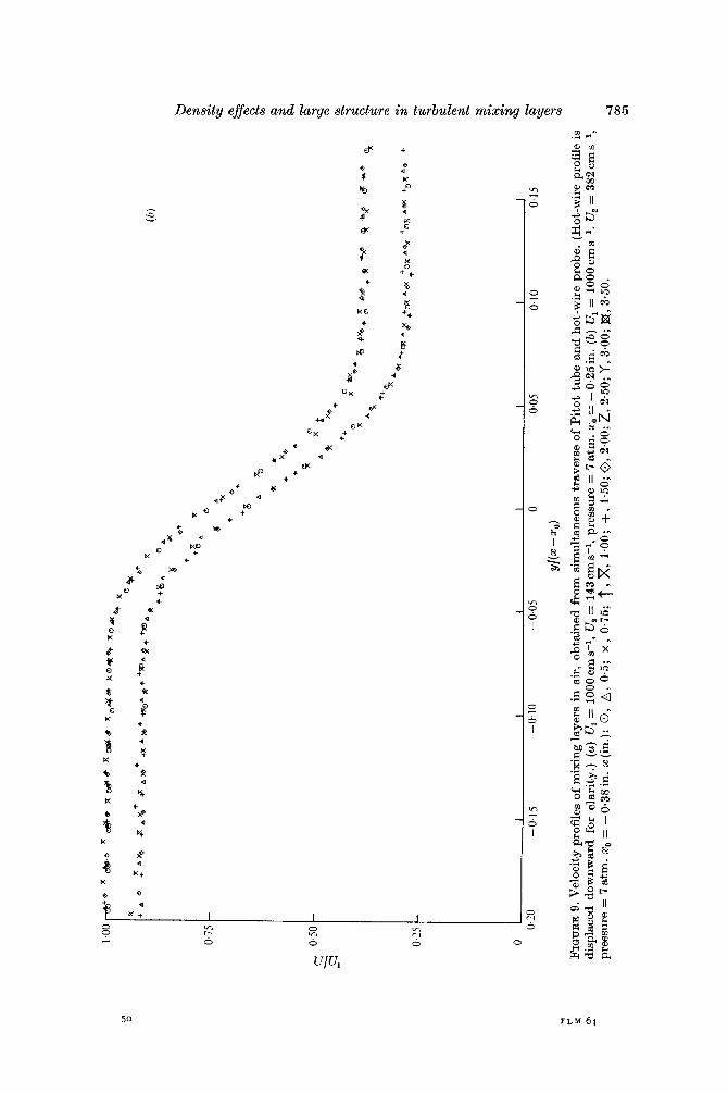
The measurements were made a t a pressure of 7atm and a velocity U, of 1000 cm-l. Having set the pressure to be uniform, by adjusting the side walls, a Pitot-static tube and a hot-wire anemometer were traversed side by side (0.5 in. apart) across the mixing layer. Thus any effect of the Pitot probe’s slower response time or of other differences in the averaging of each probe would be apparent. I n each case approximately eight traverses at various locations (x) from 0.5 to 4in. downstream of the splitter plate were made. For each run a traverse of 1.5 in. (or less) produced some 1500 measurements for each probe and a mean profile was found by fitting, in a least-squares sense, a high-order polynomial (16 to 20) to all 1500 points (see discussion in 9 6). Figure 9 (a) is a similarity plot from the resulting Pitot-tube profiles for all 10 runs a t the velocityratio U,/U, = 3. The origin of x for this plot was found by fitting a straight line to a plot of the thicknesses determined at each traverse. For this flow the effective origin was at xo = - 0.25 in. (i.e. upstream of the splitter plate edge). Deviations on the low- speed side are larger than on the high-speed side, partly because the relative fluctuation level is much larger on the low-speed side, partly because the Pitot pressure is only 2 yo of its free-stream value, which makes for larger relative errors in measurement. Even less scatter was obtained for the velocity ratio of 1: J7 (figure 9 ( b ) ) .

Ln

1 .oo

0.75

0.50

.

s

0.75

0 I

I I

I I

I I

Y/(

X - 20

) LJ

r z 0

1

FIG

UR

E

9. V

eloc

ity

prof

iles

of

mix

ing

lay

ers

in a

ir,

ob

tain

ed f

rom

sim

ulta

neou

s tr

aver

se o

f P

ito

t tu

be

and

ho

t-w

ire

prob

e. (

Ho

t-w

ire

prof

ile

is

disp

lace

d do

wnw

ard

for

clar

ity

.) (a) U

, = lO

OO

cms-

', U

, = 1

43cm

s-',

pres

sure

= 7

atm

. xo

= -0

.25

in.

(b) U

, = 1

OO

Ocm

s-1,

U, =

382

cms-

1,

pres

sure

= 7

atm

. xo

= -

0.3

8in

. x

(in

.): 0

, 8,

0.5;

x

, 0.

75; t,

x, 1.0

0; +

, 1.5

0; 0

, 2.0

0; z, 2.5

0; Y, 3

.00;

B, 3.50.


+ 0

I 1 I I I I I I I 0.5

FIGURE 10. Vorticity-thickness dependence on velocity-difference parameter for uniform density. Results of various investigators: A, present; , Liepmann & Laufer; 0, Miles & Shih;O, Mills; 1, Patel; x , Pui; 0, Reichardt (see Schlichting 1960, p. 599); +, Spencer & Jones; 4, Sunyach; [7, Wygnanski & Fiedler; A, Yule.

Shown on the same figures but displaced vertically are the profiles measured with the hot-wire anemometer. The correspondence between the profiles measured by the two methods is very close. I n the case of the hot-wire measurements, the (nonlinear) voltage-velocity calibration curve was included in the computer program for reducing the data. That the Pitot-tube results agree closely indicates that any possible nonlinear contribution due to fluctuations is negligible.

The values of vorticity-thickness spreading rate S: determined from these profiles are 0.134 and 0.089 for r = 3 and 11 J7, respectively. They are plotted in figure 10, along with values determined from the data of other investigators, against the parameter A, introduced below. On the basis of this, we believe that the mixing layers developed in the flows in this apparatus are not different from those measured by other investigators in more conventional flow systems. Our measured points are well within the scatter band of the collected measurements.

This scatter is, in fact, rather larger than would be desirable if the data were to be used to define the dependence of spreading rate on velocity ratio (i.e. 8: =

G(r ; 1)). Various proposals for a function of this type have been put forward by various investigators. Amongst these is the relation

Density esfects and large structure in turbulent mixing layers 787

proposed by Abramovich (1963) and Sabin (1965). co is a ‘standard’ value a t r = 0. The corresponding relation for the vorticity-thickness spreading would be

s:/s:, = cjc, = A. ( 5 . 2 )

The motivation for plotting the data against A, rather than r , comes from this relation. However, there are several important points about the adoption of this variable, as well as the method of plotting, which need to be discussed.

First, many authors have used ale, as the dependent variable; this tends to increase indefinitely as r +- 1 or h -+ 0. As pointed out by Birch & Eggers (1972), following a suggestion by S. J. Kline, it is more sensible to use co/c, or in our case S:/S:s, because then the very good point a t the origin ( A = 0) can be used for anchoring any curve through the data. The perfectly reasonable assumption is that turbulent spreading rate will tend to zero for zero velocity difference between the two streams. Of course, in reality the initial boundary layers from the splitter pl te become dominant for U, = U, and the flow becomes a wake flow. For U, only sli 2h tly different from U,, it is necessary to be very far downstream for the wake component to give way to a pure mixing layer flow. It is for this reason, probably, that the experimental data tend to show rather large scatter for h --f 0. The anchor point a t the origin is very helpful for steering the curve through this portion of the plot.

There is another region of large scatter, namely at U, = 0. This brings us to our second point about the method of plotting. To plot the data in normalized form, in terms of some particular value (T, or S;, a t U2 = 0, is to put an unnecessary bias into the data fitting, particularly in view of the large scatter a t U2 = 0. We have therefore chosen, in figure 10, to present the data without normalization, leaving open for the moment the question of the best curve through them. The reasons for the large spread here may be connected with difficulties of measuring on the low- speed side of a layer for which U2 = 0 (but this should not affect the determination of maximum slope thickness); or they may be connected with sensitivity to the environment on the low-speed side. (It may be noted that the case U2 = 0 is somewhat singular, in that the entrained flow velocity has a magnitude of about 0.035U1, and is not parallel to the velocity U,, but more nearly perpendicular to it.) Whatever the reasonsfor the scatter a t U, = 0, anaccurate determination a t this point is important for helping steer the curve through the region near h = 1. In view of the scatter, a straight line through the origin would appear to be as good as any for fitting the data in figure 10 (i.e. to use the Abramovich-Sabin relation). The best-fit line (r.m.s. deviation = 0-015) has the equation

u - u, 1 - r 8: = 0 . 1 8 1 1 = 0.181- = 0.181h. u, + u2 l + T

(5.3)

This curve intersects U2 = 0 a t S:, = 0.181. The mean value of all the data a t U2 = 0 gives a slightly smaller value, 8:o = 0.178.

However, we tend to be prejudiced in favour of an even lower value of &Ao, one closer to the Liepmann & Laufer (1947) value of 0.162, recently checked very closely by Spencer & Jones (1971); the scale and the Reynolds number in these two experiments was larger than in most of the others. But if the curve is to pass

50-2


through a value of about 0-16 a t h = 1, then a straight line through the origin will not be a very good fit to all the data. A curve which is concave downward would be indicated. Some indication of this tendency is also evident in the plot of 6& in figure 7. Yule (1972) also argued for a curve concave downward and proposed a relation of the form

To pursue this idea further, it is instructive to discuss possible modifications of the Abramovich-Sabin relation. Consider first a hypothetical experiment in which the two half-spaces of fluid separated by the plane (y = 0, z = 0) are impulsively set iqto motion at time t = 0 with velocities Ul and U2, respectively. Initially, this is &he problem of the temporal instability of a vortex sheet. The interface will become turbulent and, in the usual way, viscosity not being explicitly a parameter of the turbulent shear layer so established, the thickness of the latter must ultimately grow according to the law

6 = const. (U, - U2) t. (5.4)

Whatever the values of the velocities Ul and U,, only the velocity difference is significant in this temporal problem, which is invariant to a Galilean transformation. This statement cannot be made for the spatial problem, which is the subject of this paper, and of any steady-flow experiment. As in stability theory, one might try to ‘transform ’ from the temporal to the spatial problem by a relation

t = XI&,

where V, is an effective or convective velocity. For example, if we choose for this the average velocity U, = *( Ul + U2) then

6 u,- u2

X ul+ U,‘ - = 6’ = const.-

This is one way to derive the Abramovich-Sabin relation. One might make other choices of V,, e.g. the velocity of most-amplified

instability waves in a shear layer. Another possible choice for V,, but no more rigorously founded than the others, is the velocity U, on the dividing streamline ($ = 0 ) , which has values equal to (for U, + 1) or greater than the average velocity. A fairly accurate, explicit formula for U, can be obtained by representing the velocity profile by a straight line,

U(Y) = u2 + P1- 7-42] YP,

and using the formula of Korst, Page & Childs (1955) for locating the dividing streamline. The result is

Using this value of U, for CL results in

6: = const. h( 1 + QhZ)-t. (5 .5)

Density eflects and large structure in turbulent mixing layers 789

To fit the data in figure 10, we would choose const. = 0.202. The curve is concave downward and passes through &Lo = 0-1 75 at h = 1.

A more accurate representation of the velocity profile shape would alter this result only slightly. A more useful additional step would be to extend the calculation to the case of different densities, s =i= 1, but for this it would be necessary to determine a suitable density-velocity relation p = p( U ) . So far we have not attem ted this.

eddy-viscosity model. This was the basis of Sabin’s derivation. If it is assumed that the velocity profiles, for various values of U2/Ul, may be written in the form

Yet P another result for the velocity dependence of 6‘ may be obtained from an

and that the eddy viscosity vT is of the form

vT = const. 8(U, - U,),

then a similarity solution to the equations may be found in which f (yl8) depends (weakly) on U2/Ul. The first term of an expansion solution of the integral form leads to the result 8; = const. A, and inclusion of the second term results in

6: = const. [h/( 1 + ,,hz)]. 8

The data in figure 10 can be fitted with a constant of 0.204, thus &Lo = 0.174. On the basis of accuracy of fit, it is not possible to distinguish between the

three formulae proposed above. The accuracy based on r.m.s. deviation is in all cases 0.015 (i.e. about 8 yo). To decide between the straight-line Abramovich- Sabin relation and the concave-downward curves which the other models suggest, it would be helpful to have a more certain value of 8; at U, = 0. The dispersion in the seven values at U, = 0 that we have used, as may be seen on figure 10, is very large (the mean value is 0.178 with r.m.s. variation of 0.024). Until the scatter in the values, especially a t U, = 0, can be narrowed, there appears to be no basis for preferring one formula over the others. Accordingly, in the discussion of density effects in 336-9, we shall use as reference curve for uniform density (s = 1) the simple Abramovich-Sabin relation in (5.3). That relation was also favoured by Birch & Eggers (1972) for their correlation of the spreading parameter a,/a; however, they left open the question of the constant.

To summarize, the agreement of our results with those obtained in a variety of other experimental situations lends confidence that the apparatus produces ‘normal’ free mixing layers. On the other hand, it must be admitted that the collected experimental data have an undesirably large scatter, so that the definition of the important function &:(A) is somewhat uncertain. Attempts to formulate models for deriving the function, as well as the experimental data, suggest to us that the function is not linear, but concave downward. However, the data are not accurate enough to allow a conclusive judgment, and it seems appropriate for now to use the simple straight-line fit in figure 10. How much the


density ratio p2/p1 influences the growth rate is the subject of $6 6-9. In trying to evaluate this influence, we shall assume that SJh) for uniform density is defined by (5.3).

6. Results for density difference Using the procedures described in $ 5 for uniform density, measurements were

made in the mixing region between nitrogen and helium. I n addition to the Pitot- static probe used for measuring dynamic pressure, the traverse carried a density probe which could measure the local composition of the gas (i.e. the concentration of helium relative to the nitrogen). This probe, which is described by Brown & Rebollo (1972), has a response time of about 0.2 ms and samples a volume of a few thousandths of an inch in diameter. It is insensitive to velocity when the Mach number is small, as in our experiments.

The output during a traverse of the composition probe is shown in figure 11 (u). I n this computer plot the voltages put out by the probe have been converted to densities by means of a calibration obtained for various mixtures in a static system. The plotter connects the data points with straight-line segments, which gives the impression of a continuous signal. The plot is actually a series of discrete outputs, one from each sampling point as explained in 5 3. It may be seen that the fluctuations of density, or composition, are large, a point to which we shall return later. For the present, we are interested in mean values. It may be noted that the measured density is nowhere greater than that of nitrogen or less than that of helium. The small fluctuations at the nitrogen and helium levels outside the mixing zone are noise. To determine the mean density profile from the distribution of instantaneous values shown in figure 11 (u), the following method was adopted. A high-order polynomial (up to 20 terms) was fitted to the data (1500 points) by determining the coefficients for a best mean fit in the least-squares sense. Experimentation with the number of terms in the polynomial suggested that the procedure gave accurate results and this was confirmed (Rebollo 1973) by comparison with time-averaged values obtained from stationary probes. Mean density profiles determined in this way are presented in following figures.

Figure I1 ( b ) shows an example of the dynamic pressure recorded during a traverse of the Pitot-static probe where, because of the damping of the probe- transducer system, the recorded signal has much less fluctuation. These profiles were smoothed in the same way as the density profiles.

There are two possible ways to determine the mean velocity profiles from the measurements of density and dynamic pressure. One is to compute the velocity squared a t each step by dividing the Pitot-static tube signal by the density-probe signal, then smooth the resulting data, and this was done a t first (Brown & Roshko 1971). The other method is to determine the mean velocity profile from the mean profiles of dynamic pressure and density. An analysis of the expected errors from cross-correlation terms (Rebollo 1973) indicates that the latter method is somewhat more accurate and, without any attempt at including correction terms for the cross-correlations, gives mean velocities accurate to about 4 yo. The mean profiles of density and velocity determined in this way


from the data in figure 11 are shown in figure 12. Also shown is a density profile obtained by averaging groups of 50 adjacent points.

Using these methods, mean density and velocity profiles were determined a t several values of x downstream of the splitter plate. Various characteristic thicknesses could be defined for each profile. A plot of any of these against X ,

fitted by a straight line, defined the value of xo a t the intersection of the straight line with the x axis. Consistent:values of xo were obtained when different definitions of thickness from the different profiles (density, dynamic pressure, velocity) were used. With xo determined, the mean density and velocity profiles were plotted against y/(x - xo) and the similarity profiles so determined. These similarity plots for three different flows are given in figure 13. The three flows are mixing layers between helium and nitrogen streams for which the parameters correspond to p1 Ul = p2 U,, p1 UZ, = p, UZ, and p1 UZ, = 49p, Ui , in parts (a)-(c) of the figure, respectively. The case p1 Ul = 49p, U, is not given because accurate measurements could not be obtained, the corresponding ratio of dynamic pressures across the layer being 343 !

We noted previously the effect of density difference on spreading rate as determined visually from pictures. The results are given in figure 7 . Plotted on the same figure are points labelled 8;) which are determined from the mean density profiles, taking SP as the thickness between the edges (within 1 % of the free- stream values). It may be seen that the spreading of the density profile coincides fairly well with the extent of mixing visible on the shadowgraphs.

A similar plot for the vorticity thicknesses, determined from the velocity profiles, is given in figure 14. The two data points for p2/p1 = 7 and one point for p2/p1 = 3 are too few to warrant any inferences about the shape of the curves for those values of density ratio, and we have simply fitted straight lines through the origin. Comparing with figure 7 , it may be seen that the effect of density ratio on 8: is about the same as on S& From the intersections of these lines with h = 1 we infer the effects of density ratio a t U, = 0, for comparison, in $ 7 , with supersonic effects.

7. Discussion of density effects The relationship between the shear layer parameters and the density ratio in a

supersonic shear layer has been the subject of many theoretical and experimental investigations. Some of the popular theoretical approaches are based on the assumption that the main role of compressibility effects a t high Mach number is to set the temperature and density profiles; and they seek e.g. a transformation to the case of uniform density. All transformation methods of this Howarth- Dorodnytsin type have implicit in them the assumption that the effect of density non-uniformity is universal, whether it be due to compressibility, or incompressible variation of composition, or incompressible non-uniformity in temperature. For laminar flows these transformations develop rigorously and provide useful methods of solution of the compressible equations but for turbulent flows, for which the laws governing the Reynolds stresses and other transport terms are not known, this method requires empirical inputs. I n particular, it may be


i


- 0 1 t-:

s i

Q, P-

al m

+ F a x +

+ 6 Q X +

+ 6*

6

+*x

X

G . L. Brown and A . Roshko

+

6 +

6 +

8 +

F +

: t 3 3

6

+** +a + x

+ 4 + *

+ x 6

0.75

0.50

0.25

0

0 +

*??

+A

60

R D

*i

+ f

+:

+a

+lb

d D

D +

*p

-0.1

5 -0

.10

-0.0

5 0

0.05

0.

10

0.15

Y/(

X - 20

)

FIG

UE

E

13. P

lots

of m

ean

dens

ity

and

vel

ocit

y pr

ofil

es in

sim

ilar

ity

co-o

rdin

ates

. Fo

r al

l cas

es, U

l =

100

0 cm

s-l

, p =

7 a

tm. (

a) He-

N,:

Ul =

7 U,,

pl=

~p

,,~

,=0

~0

5in

.x(i

n.)

:0,0

.50

; +

,0.7

5;

o,l

.OO

;T,1

.50

; x

,2.0

O;x

,2.5

0; n

,3.0

0; Z, 3.50

. (b)

He-

N,:

U,=

7*

Uz

,p1

=~

pz

,z0

=-0

~4

0in

. 2 (

in.)

: +

, 1-0

0; T

, 1.5

0; 0,

2.00

; A, 3.

00;

x , 4

.00.

(c)

N,-

He:

U

, = 7

3U,,

p1 =

7p2

, xo =

- l.O

in.

z (h.): 0,

0-75

; x , 1

.00;

T, 1

.50; 0

, 2.0

0;

+ , 3

.00;

8,

4.00

.


1 1 1 1 1 1 1 1 1

FIGURE 14. Effect of density ratio on spreading rate.

expected that compressibility, especially a t high Mach numbers, will have an important effect on the turbulent structure (apart from effects on the density distribution) and thus on the Reynolds stresses, etc. Such problems are the subject of this article.

I n 9 7.1 we compare the results of our measurements of turbulent spreading rates a t low Mach number with results of other investigators a t supersonic speeds. It appears that there is an essential difference between these two cases for the same density and velocity ratio. We then show in $9 7.2 and 7.3 that the observed differences may be related to the forms of the Reynolds equations for incompressible and supersonic flow. It is found that the pressure-velocity correlations can account for the observed difference between shear layers in supersonic and incompressible flow, and estimates incorporating this correlation qualitatively describe the dependence of spreading angle on Mach number for supersonic flow. I n fact, if the correlations u12)) and p" depend only on density and velocity differences, and not specifically on Mach number, it is only the pressure-velocity correlation which can account for the observed difference. Finally, in $7.4 we discuss the observed difference in spreading rate of the density and velocity profiles in incompressible flow. This can be described by an eddy-viscosity model only if the Schmidt number is much less than 1 (in our case approximately 0.3).

7 . i. Comparison with supersonic mixing layers

One of the initial aims of this work was to compare the effect of density on turbulent mixing in supersonic and subsonic flows. This comparison is made in


0.1 0.2 0.4 0.6 0.8 1 4 6 8 1 0

P 1IP 2

FIGURE 15. Effect of density ratio on spreading rate with U, = 0. 0, values for incompressible flow (from figure 14). Other symbols are for compressiblemixinglayers: + , Maydew & Reed (1963); A, Ikawa (1973); x , Sirieix & Solignac (1966).

figure 15, where the present results for growth of vorticity thickness in incompressible flow are plotted against density ratio, together with the results of other investigators in supersonic flow. Clearly, the thinning of the mixing layer with increasing density on the high-speed side is much stronger in the supersonic case. It must be interpreted as an effect of compressibility connected with the Mach number, which is marked off on the density scale. (For all the flows cited the density ratio p1/p2 G KITl, where T, is the adiabatic recovery temperature.)

In incompressible flow, a density ratio p1/p2 = 7 decreases the vorticity thickness by about 30% compared with the uniform-density case, whereas, in supersonic flow with the same density ratio, the vorticity thickness is decreased by a factor of about 300 yo (estimated by extrapolating the data to Ml = 5-7) compared with the incompressible, uniform-density case.

7.2. Governing equations

For both supersonic and incompressible, variable-density, plane turbulent mixing layers the same continuity and momentum equations apply:

a a - ( p U ) + - ( p n j v ) = 0, ax aY

a a a - -(pU2)+-(pUV+ U p " ) = --(pu'w'), ax aY aY

a - ap - (pv'2) = - - . aY aY


(The usual approximations, that gradients in the x direction are small compared with gradients in the y direction, and that r.m.s. values of the fluctuations u' and v' are comparable, have been made. It is understood that all the variables are time means.) If the correlations and u- depend only on density and velocity (and not specifically on temperature or Mach number) then the experimental difference between the supersonic and incompressible variable-density shear layer must arise from differences in the other equation to be satisfied, namely the energy equation in variable-temperature flows, and the diffusion equation in variable-composition flows.

The diffusion equation for the i th component of a mixture of gases is found from the conservation of molecules,

ani -+V.n,u, = 0, at (7.4)

where ni is the number of molecules of the i th component per unit volume and u, is the average velocity of the particles, and Fick's Law, i.e.

n, n. -(u,-u) P = -g@v--", P (7.5)

where 9 is the coefficient of diffusion, p the density, and u the velocity of the centre of mass of the mixture of particles (Hirschfelder, Curtiss & Bird 1954).

These two equations combine to give the diffusion equation

an, -+V.n ,u=V. at

In the particular case of diffusion in uniform-temperature subsonic Aow, the variation of thermodynamic pressure and temperature throughout the flow is small (i.e. Aplp, A T / T are of the order of M2). Summing the partial pressures at any point then gives p = nkT, where n is now Cn,. Thus the variation of n throughout the flow is small (i.e. Anln N ill2).

Summing equation (7.6) over all components in a low-Mach-number flow therefore leads to the general unsteady diffusion equation

v.u = V.(pg@Vl/p). (7.7)

For a turbulent flow we now write u = U + u' and the same reasons that lead one to postulate a large Reynolds stress relative to the viscous stress also lead to the omission of molecular diffusivity; (7.7) reduces to

V . U = 0.

This is simply the statement that the flow is incompressible; at low Mach number, the volumes of fluid particles remain constant. Thus, to the extent that molecular interdiffusion is negligible, turbulent mixing may be viewed as a complex 'entanglement' of fluid elements which maintain their volumes and identities.

To summarize, for a steady two-dimensional turbulent flow of variable com-

Density eflects and large structure in turbulent mixing layers 80 1

position the equations of motion are continuity and momentum (7.1)-(7.3) and the diffusion equation, which reduces to

au av -+- = 0 ax ay

( U and V being time-averaged velocities of the centre of mass of the particles a t any point). By defining p 8 = pV +p" and eddy diffusivities gT and vT, where

(7.1), (7.2) and (7.8) can be rewritten in the forms

(7.9), (7.10)

(7.11)

(7.12)

(7-13)

which are identical to the two-dimensional laminar boundary-layer equations with V replaced by 8, and molecular diffusivities replaced by the eddy diffusivities vT and gT.

Now with the supersonic shear layer in mind, but generally for any uniform- composition variable-temperature shear flow (in the boundary-layer sense), the diffusion equation (7.7) is replaced by the energy equation

Por a perfect gas (h = ~ / ( y - l ) p / p ) , (7.14) can be rewritten as

(7.14)

(7.15)

Using the continuity equation and substituting for Dp/Dt gives the general two- dimensional ' boundary layer ' energy equation

For a turbulent flow P +p', U + u', etc. are substituted for p and u, etc., in this equation; for the steady plane shear layer the resulting mean energy equation reduces to

p -+- au av +- a p'v'+- - 1 v-- aP- 0, [ax a,l aY Y aY

(7.17)

where again the Reynolds number is supposed sufficiently large for the molecular diffusion of heat and momentum to be negligible. In obtaining (7.17) from (7.16) it has also been assumed that gradients in the y direction are large compared with

5 1 F L M 64

802 G. L. Brown, and A . Roshko

gradients in the x direction, that p)uI is of the same order asp-, that aPlax = 0 and .that (y- lf/yv'ap'lay is of the same form but smaller than i?/i?y(pT). This last assumption is convenient, but is by no means necessary for the argument that follows.

I n this form, it is immediately clear that, if the last two terms in this energy equation (7.17) are negligible, the equation becomes identical with the 'diffusion equation', (7.8). Then and only then would there be no distinction between the three shear layers having the same velocity and density ratio, but having the density difference across the layer due, in one case, to a difference in molecular weights of the gases on either side, in another case to a difference in temperature of these gases, or in the third case to high-speed compressibility effects. That there is a difference between the first and last of these cases must be due to the significance of the last two terms in (7.17) if the correlations ZLT and p- depend only on density and velocity differences, and not specifically on Mach number.

It will be shown in § 7.3 that the last two terms are negligible for incompressible turbulent mixing layers between streams a t different temperatures, so that in this case (7.17) becomes

au av ax ay -+- = 0. (7.18)

Again by definingpv = pV+p'v', and making use of continuity (7.1), (7.18) can be written as

Using p = pRT and noting that p is constant t o order ill2 across a turbulent mixing layer, this equation becomes

where it has been assumed that p'/p is sufficiently small for- to be equal to (p /T) T'v'; i.e. (7.18) is equivalent to the familiar incompressible turbulent-

where KT, the thermal eddy diffusivity, is defined by

(7.19)

(7.20)

To summarize, the main results of the above analysis are the following. At low Mach number, turbulent mixing is incompressible, whether the mixing streams have the same densities or not. It is immaterial how the differences in density arise, whether from temperature differences or from molecular-weight differences. At high Mach number, however, compressibility introduces effects which do not occur in the low-speed flows and which introduce into the Reynolds equations Mach-number dependent terms involving the pressure-velocity correlation 21/0)

Density efjects and large structure in turbulent mixing tayers 803

and possibly the pressure-gradient term Vaplay. This compressibility effect is distinct from any effects due to density differences which might arise from the conditions of the high-speed flow. By choosing suitable supply temperatures, it would be possible to produce a mixing layer between a supersonic stream and a quiescent ambient region (U, = 0) with densities the same in both streams (p, = pl). We expect that for given Mach number MI the turbulent spreading angle would still be approximately the same as in figure 15, i.e. much smaller than for a constant-density flow a t M 0. (In the proposed experiment, the mean density would probably not be constant throughout the mixing region.)

7.3. Order-of-magnitude estimates

Using continuity and rewriting the left-hand side of the momentum equation (7.2) in the usual Eulerian form leads to the usual estimate

- U'V' N uUAU (7.21)

for the order of magnitude of uIz)), where a is a measure of the spreading angle (AylAx) for the layer. It is also reasonable to suppose that N u'v' (where u' means the r.m.s. fluctuation level) and that u' N AU even in the compressible flow.? It follows from these estimates that

vuI N au. (7.22)

(If it is assumed that v' - u'( N A U ) it then follows that a N AUjU, which in the notation of $5 leads to the usual constant density approximation for the effect on spreading angle of different velocity ratios, namely a = const. (1 - r ) / ( 1 + r ) . )

With these estimates the orders of magnitude of terms in the energy equation (7.17) can now be made. From (7.3) Vap/ay N V(pa2U2)/(Ay), and likewise, ifit is supposed that p' is a t least of the same order as the mean variation in static pressure, then p- N p'v' or pa3U3. In terms of these orders of magnitude, the energy equation is

aAU + V + a3UM2 + Va2M2 = 0, (7.23)

where M is the Mach number U/a and a2 = yp/p. Clearly, for small Mach number the last two terms are negligible, and the 'energy' equation (7.17) becomes identical with the 'diffusion' equation (7.8). Thus, the shear layer between gases having different molecular weights will be the same as that between hot and cold streams of the same gas if the density and velocity ratios are the same in both cases.

It is clear, however, that, for sufficiently large Mach number, a must depend on M for the last two terms in (7.23) to remain of the same order as the first two. This dependence is evidentlv

(7.24)

t This assumption could be thought of as implying an oscillation of the shear layer with an amplitude equal to some fraction of the shear layer thickess. If, indeed, this amplitude is decreased at high Mach number, the dependence of a on Mach number, which we find, will be even greater.

51-2


It is interesting that this result does qualitatively describe the experimental results which are available (figure 15). A rough fit to the high-M portion of the curve might be 8; = O-2/Ml.

According to this estimate, a t high Mach number vf decreases; i.e.

a result we are not able a t present to compare with measurement. It should be noted, however, that, while v f decreases with M , so too does a, so that the turbulent terms that have been neglected in deriving the equations are still negligible.

It is interesting to note that, because of this required dependence of a on M at high Mach number, also depends on M ; i.e.

- U'V' N M-l( UAU)& AU.

This suggests the possibility that at high Mach number the form of the eddy viscosity vT defined by u'v' = - vT aU/ay should be

VT N S(X) (UAU)&M-l,

and not that for incompressible flow, for which a N A U / U and u- N AU2 give correspondingly the familiar vT N S(x) AU, where S(x) is the local shear layer thickness.

7.4. The diffusivity of mass and momentum

In all cases of shear layers between helium and nitrogen, we find that the spreading angle of the density profile is greater than that for the velocity. This is particularly marked for the case plUl = p2U2 (figure 13(a)), in which the maximum-slope thickness for the density profile is almost twice that of the velocity profile. This is important, as it implies significantly different diffusion rates for mass and momentum, a result which must be taken into account in any theoretical model constructed to calculate variable-density turbulent flows. In fact, a common assumption in many existing calculation procedures is that the diffusivities vT and gT are equal (i.e. that the Schmidt number Sc = vT/BT = 1, or at least not much different from unity).

In trying to clarify this situation experimentally, it occurred to us that the density and velocity ratios corresponding to plU, = p2U2 is an especially illuminating case to study, for the following reason. If vT = gT, the solution of the diffusion and momentum equations

is easily shown (by substitution) to be pU = const. all across the layer. It should be noted that this is the solution for any profile function for the diffusivities, so long as the function is the same for both of them. The result implies that all


I 1 I I I I I I I 1 -0.6 - 0.4 - 0.2 0 0.2

Y/@ - 5 0 )

FIGURE 16. Profiles of pU/plU,. ---- , experimental profile, corresponding to data in figure 13 (u); -, profiles from simple eddy-viscosity theory, with Sc = 0.2,0.4,0~6,0.8.1.0 and 1.2, lowest value corresponding to lowest curve.

streamlines would be parallel, not that there would be no mixing. From the continuity equation, pP = 0 and consequently pV = ~12)). The ratio pU/pl Ul is easily determined from the measurements; its deviation from const. = 1 is a sensitive measure of the extent to which Sc + 1. Figure 16 shows the experimental values of ( p U ) / p l U,) across the layer for the case p2 U2 = p1 Ul under the conditions of figure 13 (a) . The minimum and maximum values of 0.6 and 1.3 on the low- and high-velocity sides, respectively, indicate that Sc < 1. Imagine a discontinuous profile of velocity between the values U, and U2, but allow an exchange of gases between the two sides. This would correspond to Xc = 0 (no ‘velocity mixing ’). The intrusion of light gas into the low-speed side would lower pU below p2 U2 while the intrusion of heavy gas into the high-speed side would increase p U above p, U,.

It is interesting to apply simple eddy-viscosity theory for this case (i.e. vF N b ( x ) A U , Sc = v r / g T ) and numerically calculate the product pU. The details of this calculation are given in Rebollo (1973); in figure 16 we show a comparison between the calculated and measured profiles of pU for various Schmidt numbers. The agreement in profile shape could be improved by choosing a suitable profile (or an intermittency factor) for vr(y) rather than the constant value used, but this should not significantly alter the conclusion that the effective Schmidt number corresponding to the experiment has a value between 0.2 and 03-

This considerable difference in the diffusivities is related to the large structurein the flow. Owing to the large-amplitude excursions of tho layer, helium on one side of the layer is convected with little mixing to the nitrogen side and vice versa. This motion can be thought of as imposing velocity perturbations; the requirement for continuity (across a density interface) in the corresponding pressure perturbations means that these velocity perturbations will be much less in the heavy than in the light gas. Consequently, in traversing away from a low-


velocity dense gas on one side, there will be a considerable change in mean composition before the mean velocity changes significantly (see figure 12).

8. Flow structure The most interesting, and probably the most important, part of this investi-

gation concerns the coherent structures revealed by the shadowgraphs (figure 3, plate 2 ) . It seems astonishing that many years of research on mixing layers, much of it with the help of sophisticated methods of hot-wire anemometry, had not drawn a picture of such clearly defined, distinctive structures. There is often no substitute for direct flow visualization. In our experiments, the visualization was made possible by the large difference in refractive index of the two mixing streams. In the experiments of Winant & Browand (1974) on mixing layers in water, it was achieved with dyes injected into the initial vortex layer.

Whether one views these structures as waves or vortices is, to some extent, a matter of viewpoint. On high-framing-rate motion pictures, they have the appearance of breaking waves or rollers progressing downstream. When followed by the camera (as in the Winant & Browand experiment), the vortex-like structure of each ‘wave’ becomes evident. The situation is reminescent of the late, nonlinear stages of laminar instability of a free shear layer, in which the infinitesimal wave grows and distorts, tending to roll up into a vortex on the decreasing-amplitude face of each wave. Some excellent pictures of this development from a laminar instability may be found in a paper by Preymuth (1966). In this article and the following, we examine some of the properties of these coherent eddies, to gain some understanding of their role in the turbulent mixing layer.

Whereas, in the laminar instability layer, the spacing of the eddies is equal to the wavelength of the initial small disturbance from which they have developed, it is clear from all the pictures that, in the turbulent layer, the spacing increases with increasing distance downstream. The eddy diameter also increases. Com- paring a series of random pictures (e.g. figure 3, plate 2 ) , there does not appear to be a fixed repeatable pattern in the vortex arrangements; there is only a general resemblance in that the scale increases. Now it can be argued from general, similarity principles that any mean scale must increase continuously and linearly with x - xo, and thus it is necessary that the mean spacing i and the mean size of the eddies also increase smoothly and linearly with x - xo. What may not be clear at first is that the scales and spacings of individual eddies cannot possibly increase continuously. The reason is that each eddy is an identifiable entity which during its lifetime travels at a constant speed near the average +(Ul+ U2). This convective speed is independent of size or location of the eddy. It would seem, then, that the frequency with which eddies pass any station x must be invariant, but on the other hand, the requirement of increasing spacing requires a decreasing frequency. The lump of vorticity that is an eddy cannot simply disappear; thus one is led to conclude that, as they convect downstream, eddies must amalgamate in some way into larger structures, and that this process must continually recur with increasing x. The process of amalgamation was described by Winant & Browand (1974) as a vortex pairing, in which, at some stage, the tandem arrange-


* *

+*.* **

4 .t c

Frame number

/

I I I I I I I I I I I I I 1

150 7(KJ 150 300

Frame number

FIGURE 17. Trajectories of eddies. Helium at 1060crns-l, nitrogen a t 400 cms-l, pressure = 7 atm. ( a ) Crosses denote locations of eddies in the r, t plane. Each division on the time axis denotes 10 frames. Framing rate = 8000s-l. ( b ) Sequence continuing from (a) , but showing trajectories as faired lines.


ment of two successive vortices becomes unstable, and they rotate around each each other briefly and become one, the new structure then convecting downstream until the next encounter. An example of such a pairing process was seen by Freymuth (1966) in his study of the laminar instability, and Browand (1966) noted the appearance of subharmonics of the primary instability frequency in a laminar free shear layer. At that time, the phenomenon was not associated with an essential mechanism in turbulent mixing, but with the transition from the laminar regime, as indeed it is. At this early stage, the process still remembers the initial, laminar disturbance.

Although the details of the pairing are not so discernible in our shadowgraphs as in the pictures of Winant & Browand, the amalgamation events can easily be seen by plotting the trajectories of the eddies on an x, t diagram. The one case we have studied is shown in figure 17. A camera with high framing rate was used to obtain a movie sequence of shadow images, on which individual eddies could be followed from frame to frame, and plotted on the x, t plot. Figure 17 (a) shows the actual points as determined on a scanner in which the film was mounted. There is a certain amount of noise or scatter connected with the definition of the location and with measuring error. Figure 17 (b ) shows the data smoothed by eye, to give a better impression of the processes depicted. A plot of this kind was also prepared from our film strip by Damms & Kiichemann (1972).

It will be seen that the trajectory lines are all fairly parallel to each other; over all the trajectories plotted the speed varies from 0.45u1 to 0.60U1 with an ‘average’ of 0-53U1. This is significantly lower than $(Ul+ U,) = 0.69U1, but it should be noted that instability theory shows that there is a tendency to pull the wave speed toward the velocity on the high-density side ( 9 7.4). The calculation of the speeds is based on a knowledge of the framing rate ( ~ O O O S - ~ ) , which is known to about 5 yo. During its constant-speed lifetime, each eddy structure is quite identifiable, but a t some point it can no longer be followed. On the x, t plot, it can be seen that at the same time an adjacent vortex is also terminating its separate lifetime, and it seems quite clear that this must be the vortex-pairing process observed by Winant & Browand. In addition to vortex pairing, triplet and even quadruplet events also occur, but much less frequently.

From the movie strip we have been able to obtain a certain amount of statistical information, e.g. about the average spacing between successive eddies. This was determined from an ensemble of spacings between all identifiable pairs on 500 successive frames of film. At a framing speed of 8000 s-l and with a vortex convective speed of 0-53U1 = 18.5 f t s-l, this can be interpreted as a ‘ flow length ’ of 14in., compared with the test section interval of about 4in. we used. Thus the sample is not very large (e.g. at x = 3in. it corresponds to the passage of only about 15 vortices), but, averaged over all the vortices seen, the results are probably accurate to 10 yo, and should be useful for obtaining an idea of some important features.

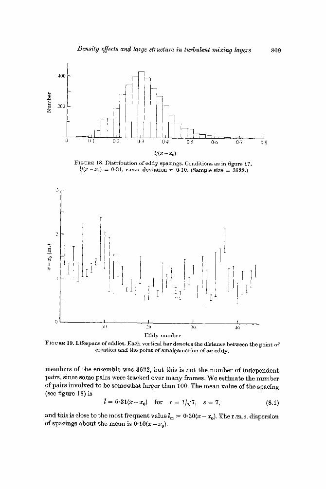
Each measurement of spacing 1 was identified with a value of x midway between the two eddies and thus a value of l / (x - xo) determined, using for xo the apparent origin determined from the profile measurements ( 3 6). The values of l/x were then sorted out into a histogram, shown in figure 18. The total number of

Density eflects and large structure in turbulent mixing layers 809

400

200

1/(x - 5)

FIGURE 18. Distribution of eddy spacings. Conditions as in figure 17. Z / ( X - x,,) = 0.31, r.m.8. deviation = 0.10. (Sample size = 3622.)

i : T ‘ 1 “I I

T I 1:

i ’ I

I i i I

I 1

I I I I I 0 20 3 0 40

Eddy number FIGURE 19. Lifespans of eddies. Each vertical bar denotes the distance between the point of

creation and the point of amalgamation of an eddy.

members of the ensemble was 3622, but this is not the number of independent pairs, since some pairs were tracked over many frames. We estimate the number of pairs invoIved to be somewhat larger than 100. The mean vaIue of the spacing (see figure 18) is

I = 0.31(x-x0) for r = 1/47, s = 7,

and this is close to the most frequent value I , = 0*30(x - xo). The r.m.s. dispersion of spacings about the mean is O.IO(x - xo).

(8.1)


Although we do not have statistical information for other values of velocity ratio and density ratio, it is clear that the constant in the above relation will vary with them. It is more likely to be invariant if a thickness rather than x - xo is taken as the reference length. Using the vorticity thickness which, for r = 1/47 and s = 7 , is 6, = 0.107(x-xn) from figure 14, we find

i = 2-96,.

We shall assume that the constant is the same for the most frequent value lnL. Changing the density ratio by a factor of 49 does not appear to change the constant greatly. On the basis of a few pictures like that in figure 5 (plate 4) we estimate = 0.21 (x - xn) and thus, using figure 14 for 6, find = 3.56,.

In their experiments with water, Winant & Browand (1974) also determined a histogram of vortex frequencies seen a t a trigger probe a t a fixed value of x. The value of the velocity ratio r = 0-36 was almost identical with ours but for their experiment in water the density ratio was s = 1 compared with our value s = 7. Using their value of the most probable vortex frequency, and assuming convection at the mean speed, gives 1, = 3.36,.

Using hot-wire anemometry, Spencer & Jones (1971) found a peak (a broad spike) in the spectra of turbulent energy a t the edges of a mixing layer in air a t a velocity ratio r = 0-6. Associating this with the coherent eddies, assuming convection a t the average velocity and taking 8, from (5.8), we calculate lm = 2-88,, but with 6, from their measured velocity profile I, = 3-38,. The values used in the latter calculation were fm = 240 s-l, U, = 1OOft s-l, x = 22 in., 6,lx = 0.036. Similarily, for r = 0.3 a t the same values of U, and x, their experiments indicate a spectral peak a t 105 s-l. With this, 1,/6, = 3.3 or 3.8, depending on whether we use (5.8) or their value for S,/(X - xo). For these same conditions ( r = 0.3), Jones et al. (1973) inferred the most probable spacing directly from space-time correlations, and found 1, = 0 . 2 8 8 ~ . With values of &,from (5.8) or from their measurements, this converts to I , = 3.86, or 5.16,, respectively. (Using a different definition for thickness, namely the distance b between the two points in the profile where the velocity is within 5 yo of U, and U, respectively Jones et al. suggest 1, = 3b as the universal relation.)

Turbulent energy spectra obtained by Kolpin (1964) in the mixing layer a t the edge of a round jet showed a maximum whose frequency decreased linearly downstream. This was not so much a separate peak as a maximum a t the low- frequency end of the spectrum, and Kolpin did not associate it with a coherent vortex structure. At this maximum, f,x/U, = 0-55. If, for this case a t U, = 0, we use U = +Ul and 6, = 0-163x, then 1, = 5-66,,. Correspondingly, 1, = 0.92x, a rather large spacing. The few pictures which we have for U, 0 (e.g. figure 6, plate 5) do not suggest that the spacing of the large eddies is as large as this, and we believe that there is still a spectral ‘peak ’ to be found for U, = 0 a t about twice the frequency of Kolpin’s maximum, possibly by looking for it in the irrotational fluctuations near the edge of the mixing layer, as did Spencer & Jones. It is interesting that peaks in the spectra, of v7 and wTobserved by Wygnanski & Fiedler (1970) in their study of a mixing layer with U, = 0 agree well with estimates using our correlations.

-


While it would be desirable to have more results, over a wide range of values of velocity and density ratio, especially for U, = 0, the above examples give some reason to believe that the mean eddy spacing in the mixing layer depends only on the mean thickness, not directly on velocity ratio or density ratio. For the present, we shall take it to be

(8.2) = 3sw,.

Another quantity of interest is the lifespan of the coherent structure. To obtain some statistical information on this, 44 different eddies with lifespans in the interval between 0.5 and 2-5 in. downstream of the splitter plate were followed. Denoting by L the distance from the point of creation of an eddy to the point of amalgamation with another one and taking its position x as the midpoint of that distance, the distribution of values of L / ( x - xo) was obtained. The mean value from this was

and the dispersion in L / ( x - xo) was 0.22; one of the lifespans in this sample was as large as 0*94(x - xo), while seven were in the lowest interval, 0.1 to 0.2(x - xo). In terms of vorticity thickness, E = 4.36,; but whether this is universal for other velocity and density ratios is not clear.

It seems remarkable, a t first, that a flow with such ‘organized’ structure, similar to the instability structure in a laminar shear layer, could have the attributes usually associated with a turbulent flow: ‘randomness ’, broad energy spectrum, etc. The usual reaction to pictures such as those displayed here is often expressed by the question, ‘Yes, but what happens when the flow is turbulent (at high Reynolds number) ? ’ That the flow is turbulent is indicated by the mean velocity and density profiles, which have the expected properties and agree well with measurements of other investigators. Also, measurements of mean fluctuating density (Rebollo 1973) show the expected self-preserving behaviour. Furthermore, shadowgraphs such as those in figure 20 (plate 7) show that the large eddy structure is not changed by changes in Reynolds number. Increasing the Reynolds number by a factor of 4 produces more small-scale structures without basically altering the large-scale. This is quite in agreement with well known views of free turbulent structure. (The enhancement of the small scales may be partially an optical enhancement with increasing pressure, but not entirely, as may be seen by comparing pictures for different Reynolds number a t the same pressure.)

In concluding § 8, we speculate briefly on what mechanisms are at work to give the flow its turbulent attributes, maintaining the point of view that the coherent structures described above play a central role.

One mechanism, of course, is the well-known ‘cascade to higher wavenumbers’, which fills out the high-wavenumber end of the spectrum of eddy sizes. We visualize this mechanism as connected with ‘internal instabilities ’ (i.e. internal to the large eddy), rather than breakdown of the eddy into smaller ‘pieces ’ (quite the opposite process is at work). The sort of thing we have in mind is illustrated in some pictures obtained by Pierce (1961) of small-scale instabilities on vortex layers which have rolled up into a large structure. Three-dimensional vortex stretching effects would also fall into this category of internal instabilities.

= 0.39(x-x,) for r = 1 4 7 , s = 7,


Of more interest, however, is the energy containing, low-wavenumber end of the spectrum. We have already seen that the scales associated with the coherent structures are quite broadly dispersed about a mean value. The measurements of Spencer & Jones (1971) show that there is a corresponding broad peak in the velocity-fluctuation energy spectrum. But the measurements also show large energy content a t much lower wavenumbers. To what are those large scales related? We believe that they are associated with what might be called ‘external instabilities ’ of the basic, coherent structures (i.e. instabilities in the arrangement of the structures along the mixing layer). The principal instability appears to be the pairing process described by Winant & Browand (and occasional multiple amalgamations). Each such process produces locally a dislocation in the vortex train. Furthermore, these processes occur at various points up and down the train. The distances between such events, say, or the times between them at a given location, define scales at wavenumbers lower than those connected with the mean spacing of the coherent structures.

In contemplating how one might model the behaviour of such an array of convecting, coherent structures, whose individual scales can increase only by discrete jumps but which on average will produce the smooth, linearly growing mixing layer required by global considerations (the Reynolds equations), it becomes apparent that there must be irregularity or ‘jitter’ in the occurrence of the discrete events. Since there is a continuity of (mean) scale along the layer, every discrete scale of the coherent structures must participate in an amalgamation event at some time or other. The mechanism for ensuring this must be interactions between the large structures up and down the layer. It seems likely that jitter would result from the amalgamation events, from the corresponding dislocations created at various points along the train and the necessary adjust- ment of the surviving vortices to such situations. All this would be instrumental in producing dispersion.

The notions we have tried to express here are still vague. A better understanding of the interactions of the large structures would, we believe, be helpful in formulating more physical models of turbulent shear flow than those based on the Reynolds equations.

In all the above, it has been implied that the coherent eddies and their interactions are basically two-dimensional. That velocity fluctuations in the spanwise direction contain energy, even a t low wavenumbers, is clear from the hot-wire measurements of many investigators. The tendency toward isotropy in the small scales is well known ; a description of the tendency toward three-dimensionality, though not necessarily toward isotropy, in the large scales is needed. Nevertheless, we believe that many of the interesting features of a plane mixing layer are described by viewing the coherent eddies as nearly two-dimensional rollers. Spanwise coherence over a few diameters should be sufficient for this. In the following article some further development of this view is used to obtain an estimate of entrainment rate.

Density effects and large structure in tarbulent mixing layers 813

9. Entrainment and mixing The use of dissimilar gases on the two sides ((i) and (ii)) of the mixing layer made

it possible to make some observations of the processes of mixing that are not revealed when the flow is homogeneous in its physical properties.

From the shadowgraphs it can be seen that the fluid on one side of the mixing layer makes deep incursions into the other side. This is confirmed by the plot of densities sampled by the aspirating probe as it traversed the mixing region (figure 11 ( b ) ) , which shows fluctuations of density almost equal to the density difference. Considering that the probe response is not perfect, it may be concluded that pure gas from each side penetrates to the centre of the mixing layer and even deeper. It is clear then that the mean density or concentration profile tells little about the degree of intimate, molecular mixing at various points of the profile. There must be rather little mixing in this sense. In fact, in turbulent mixing between two ideal fluids with zero diffusivities there would be no mixing in the molecular sense. The two fluids would remain permanently separated by the interface, which would, however, be highly convoluted owing to the instabilities that drive the turbulent process. Thus, even though not inter-diffused, the two fluids would be intricately entangled. If we now ‘turn on’ the diffusivity and viscosity (which are small a t high Reynolds numbers), the effect will be to smear out the interface and the smallest convolutions (eddies), but not to affect the large structures that determine the basic mean properties of the flow.

Closely related to this process of turbulent mixing is the phenomena of entrainment, i.e. the rate of ingestion of non-turbulent fluid into the turbulent region. One view of the entrainment process sees it as the propagation of the ‘turbulent interface ’ into the non-turbulent fluid. (This is not the two-fluid interface to which we alluded above, but the ‘edge’ of the turbulent region.) While this description may have its uses, it tends to be misleading, implying a process of ‘nibbling’ (at the edges) rather than one of ‘gulping’ or enfolding, which flow visualization shows. The process of entrainment might better be called ‘entanglement’. The entanglement appears to occur primarily in the formation of the large coherent eddies. The smaller instabilities embedded in the large structure add nothing to the basic ingestion of fluid, but only to its ‘digestion’. Thus each eddy contains and is transporting fluid from both sides of the layer which has been entangled into it in earlier stages (mainly amalgamation events) of its formation. With this view, we can make an estimate of the rate of entanglement, by assuming that the entangled fluid is contained wholly within the coherent eddies, and making use of the statistical properties we have discussed in previous sections.

Assuming each eddy to be a cylindrical structure with diameter equal to &iZ ( 9 4)) the volume of fluid (from both sides) entangled into such a vortex, per unit span, is $ 7 ~ & $ ~ . If the average frequency with which vortices pass a given station x is denoted by f ( x ) , then the average entangled flow rate is $d$, f . We shall replacefby L$, where &is the convection speed, and iis the average spacing.


(Strictly speaking,f = (VZ) + (l/l).) Thus we write for the flow rate of entangled fluid

Using (8.2) for i, (5.2) for 8, and (4.1) for Svtz, and taking V, to be the average velocity +( 1 + r ) U,, leads to

Q, = @qiZ qli.

This formula accounts for all the entangled fluid, and does not distinguish between the twosides (i) and (ii). The rates of entanglement of fluid fromeach side many be written as a, Q, and a2 Q,, respectively, with a, + a2 = 1. For the present, we shall assume a, = a2 = 4. Thus the flow rate from either side of fluid that has become entangled in the mixing layer is one half that in (9.1).

A test of this result may be made by considering the case U2 = 0 (i.e. r = 0). In this case, all the fluid from side (ii) that becomes entangled is also the fluid that is entrained, in the usual terminology. It is known that the entrainment rate must be supplied by an inflow from region (ii), and demands a velocity

V( -a) = 0.035U1,

the constant here having been evaluated from the experimental results of Liepmann & Laufer (1947). From the model outlined above, the result for r = 0 is

dQ,,/dx = 0*052U1.

While the agreement is not impressive, it seems close enough, in view of the various assumptions in the model, to suggest that the underlying ideas may be correct. For values of the density ratio p2/p1 = 7 and 3, the constant in (9.2) changes to 0.070 and 0438, respectively.

10. Concluding remarks An initial objective of this work was to determine the effects of density ratio on

turbulent mixing in incompressible flow. The amount of data is not as much as we should have liked: only three data points in figure 14, and a few more in figure 7. While this makes possible some general conclusions and comparisons with compressibility effects (as in figure 15), it is not enough data for a good determination of the density dependence C(s) in (2.5). As we have seen, there is still some uncertainty even about the dependence on velocity ratio C(r ) (figure lo), even though much more data are available. Although it is already clear that the effects are relatively small (compared with those of compressibility), a more compre- hensive determination of C(s) would be useful, and it is our intention to obtain some additional measurements for it. An interesting problem is to understand how a density difference affects the large, coherent structures which control the mixing layer development. For homogeneous flow, the problem may be considered to be one of vortex kinematics (and has been set up as such in some computer studies). There seems to be no simple way to retain this point of view when there is a difference in densities, although the pictures show that the

Density ejjects and large structure in turbulent mixing layers 815

structure is still basically the same as for the homogeneous case. In the problem of Helmholtz instability of a vortex sheet the effect of density ratio on amplifica- tion rate is to effectively increase the vortex strength by (p2/p1)*; our attempts to find simple extensions of such ideas to the turbulent mixing layer have not been very successful.

On the important problem of the properties and role of the large coherent structures, there is much still to be done. The recent work of Winant & Browand describes the crucial process of amalgamation of the structures and its relation to the growth of the layer. More understanding of the larger-scale interactions resulting from those events, and their relation to the ‘turbulent ’ character of the flow, is needed. More understanding of the details of the entrainment process, what we have called entanglement, is also needed.

Obviously, the existence of these structures suggests possibilities for models of turbulent shear flows that go beyond the Reynolds-equation modelling of most present methods. Some steps in this direction have been taken by Winant & Browand (1974) and Moore & Saffman (1974, private communication).

We are indebted to colleagues and students a t the Graduate Aeronautical Laboratories (GALCIT) for many helpful discussions, suggestions and ideas, as well as assistance with various aspects of the experiments. Some of the shadow pictures are from Rebollo (1973). A short account of this work (Brown & Roshko 1971) was given a t the AGARD Conference on Turbulent Shear Flows. The work was made possible by the generous support of the Office of Naval Research under contract NO001 4-67-A-0094-0001.

REFERENCES

ABRAMOVICH, G. N. 1963 The Theory of Turbulent Jets. M.I.T. Press. ABRAMOVICH, G. N., YAKOVLEVSKP, 0. V., SMIRNOVA, I. P., SECUNDOV, A. N. &

KRASHENINNIKOV, S. Yu. 1969 An investigation of the turbulent jets of different gases in a general stream. Astronautica Acta, 14, 229.

1972 A critical review of the experimental data for developed turbulent free shear layers. Free Turbulent Shear Plows, N A S A SP-321,

BRADSHAW, P. 1966 The effects of initial conditions on the development of a free shear layer. J . Fluid Mech. 26, 225.

BROWAND, F. K. 1966 An experimental investigation of the instability of an incompressible, separated shear layer. J . Pluid Mech. 26, 281.

BROWN, G. L. & REBOLLO, M. R. 1972 A small, fast-response probe to measure composition of a binary gas mixture. A.I.A.A. J . 10, 649.

BROWN, G. L. & ROSHKO, A. 1971 The effect of density difference on the turbulent mixing layer. Turbulent Shear Flows, AGARD-CP-93, 23-1.

DAMMS, S. M. & KUCHE;MANN, D. 1972 Possible vortex motions in shear layers. R o y . Aircraft Establishment Tech. Memo. Aero. no. 1430.

FREYMUTH, P. 1966 On transition in a separated laminar boundary layer. J . FZuid Mech. 25, 683.

HIRSCHFELDER, J. O., CURTISS, C. F. & BIRD, R. B. 1954 Molecular Theory of Gases and Liquids. Wiley.

BIRCH, S.F. & ECGERS, J . M .

p. 11.


IKAWA, H. 1973 Turbulent mixing layer in supersonic flow. Ph.D. thesis, California Institute of Technology.

JONES, B. G., PLANCHON, H. P. & HAMMERSLEY, R. J. 1973 Turbulent space-time correlation measurements in a plane two-stream mixinglayer a t velocityratio 0.3. A .I.A .A. Paper, no. 73-225.

KOLPIN, M. A. 1964 The flow in the mixing region of a jet. J . Fluid Mech. 18, 529. KORST, H. H., PAGE, R. H. & CHILDS, M. E. 1955 A theory for base pressures in transonic

and supersonic flow. University of Illinois Ens. Expt. Station Rep. ME-TN-392-2. LIEPMANN, H. W. & LAUFER, J. 1947 Investigation of free turbulent mixing. N.A.C.A.

Tech. Note, no. 1257. MAYDEW, R. C. & REED, J. F. 1963 Turbulent mixing of compressible free jets. A.I.A.A.

J . 1, 1443. MILES, J. B. & SHIH, J. 1968 Similarity parameter for two-stream turbulent jet-mixing

region. A.I.A.A. J . 6 , 1429. MILLS, R. D. 1968 Numerical and experimental investigations of the shear layer between

two parallel streams. J . Fluid Mech. 33, 591. PATEL, R. P. 1973 An experimental study of a plane mixing layer. A.I.A.A. J . 11, 67. PIERCE, D. 1961 Photographic evidence of the formation and growth of vorticity behind

plates accelerated from rest in still air. J . Fluid Mech. 11, 460. PUI, N. K. 1969 The plane mixing layer between parallel streams. M.A. Sc. thesis.

University of British Columbia. REBOLLO, M. 1973 Analytical and experimental investigation of a turbulent mixing layer

of different gases in a pressure gradient. Ph.D. thesis, California Institute of Technology. SABIN, C. M. 1965 An analytical and experimental study of the plane, incompressible,

turbulent free-shear layer with arbitrary velocity ratio and pressure gradient. Trans. A.S.M.E. D 87, 421.

SCHLICHTING, H. 1960 Boundary Layer Theory, 4th ed. McGraw-Hill. SIRIEIX, M. & SOLIONAC, J.-L. 1966 Contributions a 1’6tude experimentale de la couche de

melange turbulent isobare d‘un Bcoulement supersonique. Symposium on Separated Plow, AGARD Conf. Proc. p. 4.

SPENCER, B. W. & JONES, B. G. 1971 Statistical investigation of pressure and velocity fields in the turbulent two-stream mixing layer. A.I.A.A. Paper, no. 71-613.

SUNYACH, M. 197 1 Contribution a 1’6tude des frontieres d’6coulements turbulents libres. D.Sc. thesis, L’Universit6 Claude Bernard de Lyon.

TOWNSEND, A. A. 1956 The Structure of Turbulent Shear Flow. Cambridge University Press.

WINANT, C. D. & BROWAND, F. K. 1974 Vortex pairing: the mechanism of turbulent mixing-layer growth at moderate Reynolds numbers. J . Pluid Mech. 63, 237.

WYGNANSKI, I. & FIEDLER, H. E. 1970 The two-dimensional mixing region. J . Pluid Mech. 41, 327.

YULE, A. J. 1972 Two-dimensional self-preserving turbulent mixing layers at different free stream velocity ratios. Aero. Res. Counc. R. & M. no. 3683.

.Journal of Fluid Mechanics, Vol. 64, part 4 Plate 1

PrGultE 2. Mixing layer apparatus. The wedge-shaped splittcr plate sc:pitratcs tlic: two Ilttlf- nozzles. A probe is mounted i n tlio test section from a Iiorizorital tritvtmt:. Tllc: prossurc cylinder in the upper part of t,lie photo can bc pulled dowlr over tho seal on the circular plstc: i n the lower part.

BROWN AND RORHKO (Facing p. 816)

Journal of Fluid Mechanics, Vol. 61, part 4 Plate 2

FIGURE 3. Shadowgraphs of mixing Iaycr t,alteti at random times. Liiies show rrlrthod of determining 8tlz. Channel wid th at lcft side of picture is 6 mi.

BROWN AND EOSHKO

Journal of Fluid Mechanics, Vol. 64, part 4

FIGURE 4. Shadowgraph of mixing layer in flow between nitrogen (upper) at 326 em s-l arid air at 123 cm s-l. Pressure = 7 atm.

Plate 3

BROWN AND ROSHKO

Journal of Fluid Nechanics, Vol. 64, part 4 Plate 4

FILWRE 6 . N~adowgraplis of mixing layer betwecri nitrogeii (upper) at 876 ern s-l and helium at 330cm s-1. Pressure = 4 ntm. ( ( 1 ) Single spark exposure. ( b ) Ten superimposed rxposures.

Joumal of .Fluid Nec,h,anics, Vol. 61, part 4 Plate 5

FIGURE 6. SEit~dowgraphs of mixing 1ayt.rs with vclocity ratio Uz/Ul = 3. ( a ) Helium (uppc'r) at 7J1 = 915crns-l, nitrogen at l/, = 130c1ns prossurc = 7atm. ( b ) Nitrogcri (upp~r) at 945crns-', air a t 140cin s I , pressure = 9 at,rii. ( c ) Nitrogen (upper) at 920 ems-', Iieliurn a t 140 ern s-l, pressiircx = 5 atm.

Jouvnal of Fluid Mechanics, Vol. 64, part 4 Plate 6

FIGURE 8. Spanwisc: correlations of largc striicturrs. ( ( 1 ) Two cxamplcs of signals from hot wircs located 2 in. apart spariwise at x = 2 in., y/(z - so) = - 0.09, conditions of figure 13 ( b ) . ( b ) Shadowgraph view normal to plane of mixing layrr between helium at 1000 crn s-l arid nitrogen a t 3XOcrris-', p = 7atrn.

Journal of Fluid Mechnnics, Vol. 64, p w t 4 H n t P 7

FIGURE 20. Kffects of Reynolds number. Mixing layers bet>\vceri helium (upper) and nit'rogen (lower.) with p2 Ui = p1 U : . (a ) Reynolds number is proportional to 8 x 10 (pressure = 8 atm, U, = 10Ins-'); ( b ) 8 x 5; (c) 4 x 10; (d ) 4 x 5 ; ( e ) 2 x 10.

BROWN AND ROSHKO

On density effects and large structure in turbulent mixing ...

Documents

Transcript of On density effects and large structure in turbulent mixing ...