On Computing Probabilities of Dismissal of 10b-5 ...pshenoy.faculty.ku.edu/Papers/DSS17.pdf · On...
33
On Computing Probabilities of Dismissal of 10b-5 Securities Class-Action Cases Sumanta Singha a,* , Steve Hillmer a , Prakash P. Shenoy a a University of Kansas, School of Business, Lawrence, KS 66045, USA. Abstract The main goal of this paper is to propose a probability model for computing probabilities of dismissal of 10b-5 securities class-action cases filed in United States Federal district courts. By dismissal, we mean dismissal with prejudice in response to the motion to dismiss filed by the defendants, and not eventual dismissal after the discovery process. The proposed probability model is a hybrid of two widely-used methods: logistic regression, and na¨ ıve Bayes. Using a dataset of 925 10b-5 securities class-action cases filed between 2002 and 2010, we show that the proposed hybrid model has the potential of computing better probabilities than either LR or NB models. By better, we mean lower root mean square errors of probabilities of dismissal. The proposed hybrid model uses the following features: allegations of generally accepted accounting principles violations, allegations of lack of internal control, bankruptcy filing during the class period, allegations of Section 11 violations of Securities Act of 1933, and short-term drop in stock price. Our model is useful for those insurance companies which underwrite Directors and Officers liability policy. Keywords: probability, logistic regression, na¨ ıve Bayes, hybrid model, 10b-5 security class-action cases 1. Introduction Decision support system (DSS) tools have been an integral part of effective decision making. Over the years, DSS tools have enriched managerial judgement by turning data-driven insights * Corresponding author Email addresses: [email protected] (Sumanta Singha), [email protected] (Steve Hillmer), [email protected] (Prakash P. Shenoy) Preprint submitted to Journal of Decision Support Systems October 20, 2016 Appeared in: Decision Support Systems, 94(C), 2017, 29–41.
-
Upload
doankhuong -
Category
Documents
-
view
214 -
download
0
Transcript of On Computing Probabilities of Dismissal of 10b-5 ...pshenoy.faculty.ku.edu/Papers/DSS17.pdf · On...

On Computing Probabilities of Dismissal of 10b-5 Securities Class-ActionCases
Sumanta Singhaa,∗, Steve Hillmera, Prakash P. Shenoya
aUniversity of Kansas, School of Business, Lawrence, KS 66045, USA.
Abstract
The main goal of this paper is to propose a probability model for computing probabilities of
dismissal of 10b-5 securities class-action cases filed in United States Federal district courts. By
dismissal, we mean dismissal with prejudice in response to the motion to dismiss filed by the
defendants, and not eventual dismissal after the discovery process. The proposed probability
model is a hybrid of two widely-used methods: logistic regression, and naıve Bayes. Using a
dataset of 925 10b-5 securities class-action cases filed between 2002 and 2010, we show that the
proposed hybrid model has the potential of computing better probabilities than either LR or NB
models. By better, we mean lower root mean square errors of probabilities of dismissal. The
proposed hybrid model uses the following features: allegations of generally accepted accounting
principles violations, allegations of lack of internal control, bankruptcy filing during the class period,
allegations of Section 11 violations of Securities Act of 1933, and short-term drop in stock price.
Our model is useful for those insurance companies which underwrite Directors and Officers liability
policy.
Keywords: probability, logistic regression, naıve Bayes, hybrid model, 10b-5 security class-action
cases
1. Introduction
Decision support system (DSS) tools have been an integral part of effective decision making.
Over the years, DSS tools have enriched managerial judgement by turning data-driven insights
∗Corresponding authorEmail addresses: [email protected] (Sumanta Singha), [email protected] (Steve Hillmer),
[email protected] (Prakash P. Shenoy)
Preprint submitted to Journal of Decision Support Systems October 20, 2016
Appeared in: Decision Support Systems, 94(C), 2017, 29–41.
into actionable solutions. Much of recent developments in decision making is in model-based
management support which incorporates knowledge and models for judgement and decision [1, 2].5
An example of such system includes credit approval applications that access credit scores and other
relevant information to approve/deny credit card applications. Model-based DSS finds applications
in wide variety of domains such as quality management [3], energy planning [4], project portfolio
selection [5], and others. In this paper, we aim to develop a model-based DSS for the D&O
insurance companies in the context of 10b-5 securities class-action lawsuits.10
Securities class-actions are lawsuits filed by shareholders due to violation of securities laws.
Some common class-action allegations are fraudulent disclosure, misleading forecast, violation of
securities laws, insider trading and financial restatements. It is well known that securities class-
actions can inflict serious damage to defendant’s financial health and stock market performance
[6, 7]. In recent years, nearly 35− 40% of all class-action suits allege security frauds and account15
for approximately 75% of all settlement awards [8, 9]. Since 1996, over 4,100 security class-actions
have been filed and approximately $87 billion has been dispensed in settlements 1. As a result,
virtually every public corporations in U.S. buy Directors and Officers (D&O) coverage to safeguard
its directors and officers from class-action liabilities [10, 11].
In this context, the role of D&O underwriters and risk managers becomes crucial. While20
past literatures [10, 12] provide some guidance on preemptive risk management (e.g. predicting
corporate governance risk), the reactive risk management aspects have not been well studied. In
particular, it is still an open question for the insurance companies to decide whether to ‘settle’
or ‘fight’ (on behalf of the defendant) when facing a class-action litigation. Given the high cost
of penalties, clearly, an early settlement can potentially benefit the insurance company when the25
probability of dismissal is low i.e. the lawsuit is likely to be ruled in favor of the plaintiff. This
explains why insurance companies may be interested in predicting probability of dismissal early
in the trial. To answer this research question, we propose a predictive model that can estimate
probability of dismissal at an early stage, solely based on the allegations made by a plaintiff. This
paper investigates how an enabling decision support system can lead to improved decision-making30
1〈http://securities.stanford.edu/〉
2
for the insurance companies.
There are several challenges that must be addressed while attempting to build a probability
model. The proposed model must be reliable, well-calibrated, efficient, and sensitive to error. In
order to simultaneously achieve these multiple objectives, we adopt a multi-pronged strategy, i.e.,
Markov blankets for feature set selection; root mean square errors (RMSE) as a model evaluation35
metric; reliability diagram for model calibration; and non-parametric bootstrapping for computing
standard deviation of test set errors. We also show that our model produces lower error compared
to a recent method [13]. We discuss in further details in Section 8. Note that this paper is about
building a decision tool for predicting probability of dismissal in securities class-action cases based
on a dataset of 925 instances. We find that a hybrid of two widely-used methods: logistic regression40
(LR), and naıve Bayes (NB) performs better than pure LR and pure NB for this dataset. The
strengths of our model are that it can simultaneously incorporate continuous features and features
with missing features, is efficient and yet simple to use.
Two natural questions to ask at this juncture. First, why use a hybrid model? Second, when
does a hybrid model perform better than the constituent methods?. Below we answer these two45
questions together. Referring to the “no free lunch” theorem in [14], we state that no single
computational view solves all the problems, since each one has its own domain of competence.
Hybrid models have been studied extensively in the past with respect to classification [15, 16].
It is well known that hybrid methods seek to exploit the strengths of the individual components,
obtaining enhanced performance for the combination [17–19]. [20] provides an analytical proof that50
hybrid classifier works better under some conditions. In the machine learning domain also, different
hybrid models combining generative and discriminative approaches have been proposed, such as
hybrid generative-discriminative models [21], mixed log-likelihood model [22, 23], multi-conditional
learning models [24], Bayesian trade-off [25], H-bayes model [26], and JoDiG approach [27]. [28]
compare logistic regression and nave Bayes models. Their conclusions are that asymptotically55
LR models do better than NB, but that NB models reach their asymptotic accuracy faster than
LR models. [29] observe that the generative approach enjoys better classification performance
than its discriminative counterpart when the model is correctly specified. However, when the
3

model is misspecified, the performance of discriminative model improves as the training set size
increases. Between these two extremes, there is a region where hybrid model may outperform both60
generative and discriminative techniques. This, once again, substantiates the celebrated “no free
lunch” theorem in [14] and answers our second question. To explore whether hybrid method is
always optimal for all domains is beyond the scope of this paper.
Our sole objective is to propose a model that enables D&O insurers to identify which features
contribute to the dismissal (or settlement) of a class-action and compute the probability of dismissal65
conditional on their realizations. Our model not only helps the D&O insurers to make an early
assessment of risk, but also acts as an useful tool for the future. The study also provides useful
insights to the Securities and Exchange Commission (SEC), other policymakers, and academicians
who study policy implications and implement judicial reforms.
The remainder of the paper is organized as follows. The next section contains a review of70
related works on class-action lawsuits. In Section 3, we summarize the contributions of this paper.
Section 4 describes the dataset and explains the complexities involved in data preparation. In the
subsequent three sections, we sketch the basics of NB, LR and hybrid method, their assumptions,
strengths and weaknesses. In Section 8, we describe the feature selection methodology and their
nuances. In Section 9, we present our results and compare the models. Finally, in Section 11, we75
summarize our findings and conclude.
2. Related Work
Existing literatures on securities class-actions are broadly of two types. The first category
is comprised of those which examine the effect of the U.S. Private Securities Litigation Reforms
Act (PSLRA) of 1995 on class-action outcomes and is extremely rich in content. Motivated by80
PSLRA, these papers explore which factors contribute to the dismissal (or settlement) of a class-
action and influence the settlement size conditional on settlement. The significant contributions in
this category are by [10, 11, 30–32]. We summarize some of their contributions below.
In the post-PSLRA period, [32] finds that the allegation of financial restatements makes a
case more likely to be settled, while the allegations of insider trading and misleading forecast are85
4

insignificant for the outcomes. [30, 31] study the lead plaintiff provision of PSLRA and examine
whether institutional lead plaintiff increases the settlement size. Their findings suggest that though
institutional lead plaintiff increases the average settlement, the lead plaintiff provision of PSLRA
is generally ineffective. It is learnt that (i) provable loss, (ii) total asset of the defendant firm, and
(iii) presence of an SEC enforcement action, all positively influence the settlement amount. [33]90
investigates the kind of cases that are ultimately dismissed/settled and find that security class-
action cases that allege financial restatements and SEC enforcement actions are less likely to be
dismissed.
In contrast, the second category is relatively nascent and contains very few literatures, which
focus on predicting the probability of dismissal/settlement in a class-action case. Unlike the first95
category, here we deal with probability models that can predict probabilities. The significant
contributions in this category are by [34] and [13] . Using a dataset of 155 instances, [34] employs
a logistic regression model to determine which allegations are correlated with the outcome of the
motion to dismiss and by inference, whether these allegations influence the decisions of the ruling
judges. They find that violation of generally accepted accounting principles (GAAP) and allegation100
of false forward looking guidance favour settlement, while insider trading allegation may or may
not be significant (at 5% significance level) and the courts differ in their views. The significant
features are selected based on the p-value of the regression coefficients. Though their model is
essentially a classification model, [34] only focuses on determining the significant features that are
correlated with the outcome and hence does not provide any model performance measure. As a105
result, we only qualitatively compare our results with [34].
We now turn to the work by [13], which is most relevant in our context. Using a dataset
of nearly 1200 instances and 18 features primarily from RiskMetrics,2 they propose a Bayesian
hierarchical composite model that estimates (i) the probability of dismissal, and (ii) the settlement
size conditional on non-dismissal. The portion of the model for computing probability of dismissal is110
a logistic regression model. Some of the 18 features they use are relevant for computing probability
of dismissal, and some for predicting settlement size, and it is not clear which features are relevant
2〈https://www.issgovernance.com/governance-solutions/securities-class-action-services/〉
5

for each task.
In this paper, we develop a probability model by using a recent technique, called a hybrid model,
that combines logistic regression (LR), and naıve Bayes (NB) in one model. Using a dataset of115
925 instances of 10b-5 securities class-action cases filed in U.S. Federal district courts during 2002–
2010,3 we compute the probability of dismissal based on a set of features. Rule 10b-5 violation
deals with securities fraud and appears in approximately 82% of all security class-actions filed in
last 5 years [35].
Using a new algorithm for the construction of a hybrid model, we find that only 5 features are120
significant for computing the probabilities of class-action outcomes. They are: (i) GAAP violation,
(ii) lack of internal control, (iii) whether the defendant has filed for bankruptcy in the class period,
(iv) violations of Section 11 of Securities Act of 1933; and (v) percentage of sudden short-term
drop in share price alleged in the consolidated complaint. A predictive model is proposed that
determines the probability of dismissal based on these features. In the next section, we contrast125
our work with [13] and show that our model provides higher accuracy, in addition to being tolerant
to missing data.
3. Contribution
Our work contributes to the existing literature on class-action cases in the following ways.
1. First, we define the notion of ‘dismissal’ from the viewpoint of D&O insurance company,130
which is virtually always the principal party at interest. In our model, by ‘dismissal’ (the
class variable), we mean initial dismissal in response to the motion to dismiss filed by the
defendants, and not the eventual dismissal that the earlier works have studied. This new def-
inition also complements the underlying spirit of PSLRA, which lays emphasis on heightened
pleading requirements and disallows the plaintiff from obtaining discovery prior to disposal135
of defendant’s motion to dismiss. The idea is to eliminate frivolous filings that do not sur-
vive the test of motion to dismiss. Clearly, defendant’s motion to dismiss in post-PSLRA
3〈http://securities.stanford.edu/〉
6
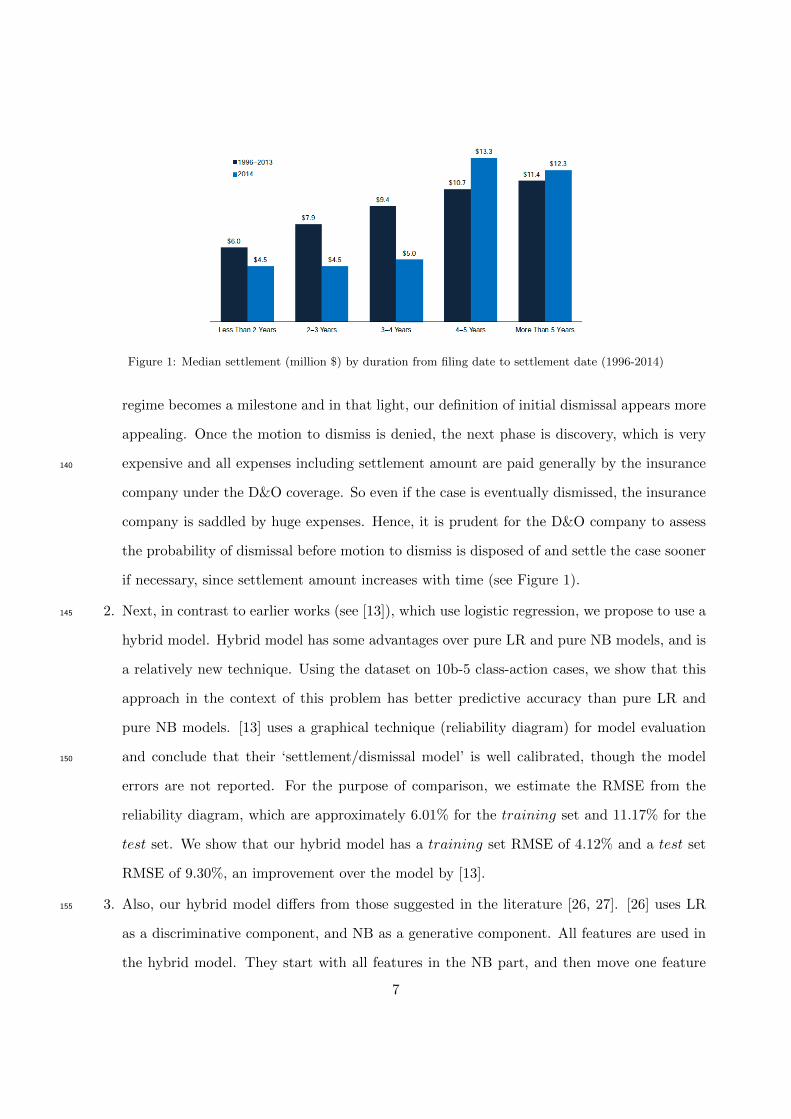
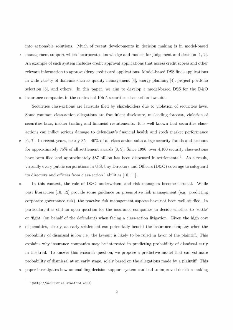
Figure 1: Median settlement (million $) by duration from filing date to settlement date (1996-2014)
regime becomes a milestone and in that light, our definition of initial dismissal appears more
appealing. Once the motion to dismiss is denied, the next phase is discovery, which is very
expensive and all expenses including settlement amount are paid generally by the insurance140
company under the D&O coverage. So even if the case is eventually dismissed, the insurance
company is saddled by huge expenses. Hence, it is prudent for the D&O company to assess
the probability of dismissal before motion to dismiss is disposed of and settle the case sooner
if necessary, since settlement amount increases with time (see Figure 1).
2. Next, in contrast to earlier works (see [13]), which use logistic regression, we propose to use a145
hybrid model. Hybrid model has some advantages over pure LR and pure NB models, and is
a relatively new technique. Using the dataset on 10b-5 class-action cases, we show that this
approach in the context of this problem has better predictive accuracy than pure LR and
pure NB models. [13] uses a graphical technique (reliability diagram) for model evaluation
and conclude that their ‘settlement/dismissal model’ is well calibrated, though the model150
errors are not reported. For the purpose of comparison, we estimate the RMSE from the
reliability diagram, which are approximately 6.01% for the training set and 11.17% for the
test set. We show that our hybrid model has a training set RMSE of 4.12% and a test set
RMSE of 9.30%, an improvement over the model by [13].
3. Also, our hybrid model differs from those suggested in the literature [26, 27]. [26] uses LR155
as a discriminative component, and NB as a generative component. All features are used in
the hybrid model. They start with all features in the NB part, and then move one feature
7

at a time to the LR part, in a greedy fashion, as long as the classification error decreases,
and stop otherwise. [27] also uses LR as the discriminative component, but use Fisher’s
(1936) linear discriminant analysis (LDA) as the generative component. All features, which160
are continuous, are used in the hybrid model. They test all features for univariate normal
distribution and those that fail are moved to the LR part with the rest in the LDA part.
4. Our method of construction is different. First, we estimate a Markov blanket (MB) of the
class variable, and eliminate features not in the MB. MB is a technique for selecting the
optimal set of features [36] for our class variable ‘dismissal’ by eliminating irrelevant and165
redundant features. [37] mentions that MB can improve the prediction performance and
speed up the training and inference process. Next, we search for a best LR model and a
best NB model from among the features in the Markov blanket, and eliminate those features
that are not used in either of the two best models. Finally, we search for the best hybrid
model (from the set of features that are either in the best LR or in the best NB models)170
with the restriction that each such feature must be used in either the LR or the NB portion
of a hybrid model. This restriction reduces the search space of hybrid models from O(3k) to
O(2k), where k is the number of features in the best LR or best NB models. In the context
of 10b-5 class-action cases, k = 5, and the search is tractable. We verify (using exhaustive
search) that such a restriction does not eliminate the best hybrid model.175
4. Data
In this section, we describe our dataset and explain the process of labeling each instance, in the
light of our new notion of ‘dismissal’. The sample is comprised of 925 instances of securities class-
action cases filed in various U.S. Federal district courts between 2002−2010. Why 2002−2010? The
Sarbanes-Oxley Act of 2002 (often shortened to SOX) is legislation passed by the U.S. Congress to180
protect shareholders and the general public from accounting errors and fraudulent practices in the
enterprise. Most of the class-action cases in 2011 onwards are still pending resolution. Our primary
source of data is Stanford Securities Class Action Clearinghouse,4 which keeps track of all Federal
4〈http://securities.stanford.edu/〉
8

securities class-action cases since the passage of PSLRA. SCAC provides historical information
of securities class action cases with accompanying full-text complaints, motions, dockets, judicial185
opinions and other major court filings. The data collection was carried out by select graduate law
students at University of Kansas, over a period of 6 months. Engaging law students is intended
to lend credibility to our dataset from legal viewpoint; making sure that the dataset is unbiased
and comprehensive. The dataset is further cross-checked with a commercial dataset (Advisen’s
Master Significant Cases & Actions Database5) for accuracy, and in case of disagreements, we190
verify by reading the consolidated complaints whether we or Advisen’s database have the correct
information.
Data collection involves two primary tasks; first, to select instances for our dataset and second,
to identify the relevant features that we use to build the model. We independently select 970
class-action cases filed between 2002 − 2010, for which the outcomes to ‘motion to dismiss’ are195
known. Our selection is not subject to any pre-determined bias with regard to industry sector,
type of plaintiff or any other attribute. Next, we select the relevant features for our model. A
total of 19 features are shortlisted, that were commonly alleged in various consolidated complaints.
Our assumption is that outcomes are merit-based and depend on the strength of the allegations
in consolidated complaint. This assumption is reasonable and consistent with the philosophy of200
PSLRA. In a pilot study carried out by [38], only 6 of these 19 features are found relevant for
predicting dismissal. Subsequently, we further add 3 additional features (last 3 in the list below).
These 9 features are:
1. GP = whether GAAP violations is alleged (1) or not (0);
2. II = whether lead plaintiff is an institutional investor (1) or not (0);205
3. BR = whether the defendant has filed for bankruptcy in the class period (1) or not (0);
4. S11 = whether violations under Section 11 of Securities Act 1933 is alleged (1) or not (0);
5. RF = whether company financials are restated during the class period6 (1) or not (0); and
6. STD = the maximum % short-term (1 to 5 working days) drop in share price alleged;
5〈http://www.advisenltd.com/2015/02/27/mscad-methodology-no-two-databases-are-the-same/〉6A ‘class period’ is a specific period of time in which the unlawful conduct is alleged to have occurred.
9

7. SI = whether investigation is initiated against the defendant by SEC (1) or not (0);210
8. IC = whether the complaint alleges lack of internal control (1) or not (0);
9. IS = whether the complaint alleges insider selling (1) or not (0);
Except STD, which is a continuous feature, all other features have binary outcomes, true (1)
or false (0), as reported in consolidated complaint. In this problem, the class variable (C) is a
categorical variable having two outcomes dismissed (d) and not dismissed (nd).215
Now, we need to assign an outcome (d or nd) to each instance in the light of our notion
of ‘dismissal’. Beyond the obvious ones where the case was dismissed with prejudice, it was
exceedingly complex to decide the outcome. We consulted with the global head of a D&O insurance
company (who sponsored this research and wishes to remain anonymous), for their expert counsel
in this matter. First, those instances, in which there the plaintiffs had voluntarily withdrawn the220
cases before defendant’s filing of ‘motion to dismiss’, were classified as erroneous filing and were
dropped. Based on this criterion, we dropped 45 cases as erroneous filings. Second, in the event
of a voluntary withdrawal of the complaint by the plaintiff, it was considered as ‘dismissed’ if
there were neither any ‘secret’ settlements (as noted in the dismissal order by the court) nor any
related filing within a year before or after the voluntary withdrawal. Third, any class-action case in225
which the defendant settles before the ruling on ‘motion to dismiss’, is deemed as ‘not dismissed’,
presuming possible merits in favor of the plaintiff. 7 At this stage, we had 925 instances left, which
were classified into 4 possible categories as described below.
Type 1: Dismissed with prejudice
In 270 such cases, the ruling judge dismissed the case with prejudice upon hearing the ‘motion230
to dismiss’ filed by the defendants. In these cases, the plaintiffs are not entitled to refile another
lawsuit for the same claim. These cases were classified as dismissed. In another 211 cases, the
ruling judge dismissed the cases without prejudice, which entitles the plaintiff the right for re-filing
another suit later on the same claim. This begins the entire process once again and follows the
7In the literature, there exist instances of ‘strike suits’ [31], in which the ratio of settlement to ‘provable loss’ isextremely low, often indicating the frivolousness of allegations. In such cases, settlement acts more as an exit routeand does not imply submission of guilt. We did not engage in such subtleties
10

same course of events. For the sake of brevity, we only summarize the results. 125 of these 211235
cases were classified as dismissed and remaining 86 cases as not dismissed.
Type 2 : Mutually settled prior to ruling on motion to dismiss
There are 176 cases in which defendants and plaintiffs agreed to settle the case before ‘motion
to dismiss’ was ruled by the judge. Such cases were classified as not dismissed indicating possible
merits in the case in favor of the plaintiff.240
Type 3: Voluntarily withdrawn by the plaintiffs
19 such cases were voluntarily withdrawn by the plaintiffs before the court’s ruling of the
‘motion to dismiss’, and hence they were classified as dismissed.
Type 4: Motion to dismiss denied
The court had rejected the defendant’s ‘motion to dismiss’ and proceeded to discovery in 249245
instances. Only 5 of these cases were eventually dismissed by the court (after a period of 3–5 years
of discovery), and remaining cases were settled by the defendant. In the light of our new definition
of dismissal, all 249 instances were classified as not dismissed.
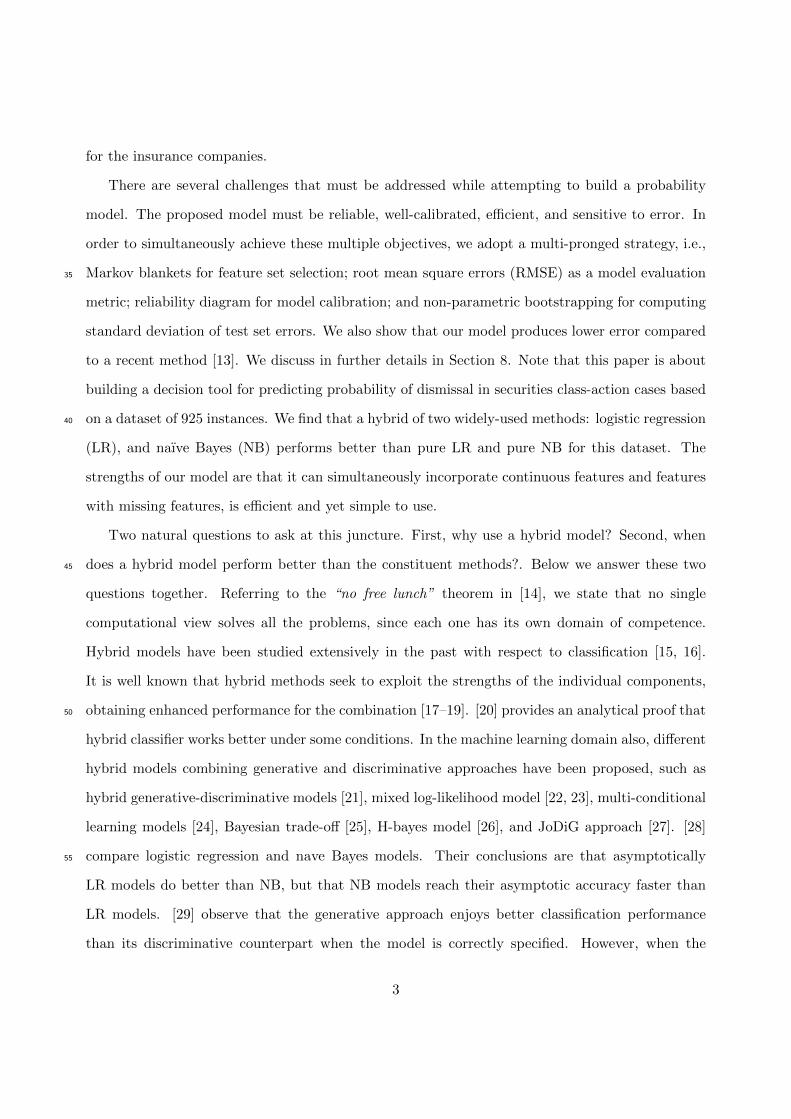
In summary, the class outcomes are as follows : # dismissed = 414, and # not dismissed
= 511. In Figure 2, we present the descriptive statistics of the 9 features across each class outcome250
dismissed and not dismissed. Short term drop (STD) is a continuous feature, but the depiction
in Figure 2 is a discretized version where STD = 1 means STD > 42.2%, and STD = 0 means
STD ≤ 42.2% (discretization of STD is described in greater detail in Section 8). There are no
instances of missing data. Finally, the dataset is randomly partitioned into a training set (90%)
and a test set (10%). As a result, the training set contains 832 cases and test set contains remaining255
93 cases.
5. Naıve Bayes
A naıve Bayes (NB) model is a Bayesian classifier that assumes mutual conditional independence
of the features given the class variable (see Figure 3). This assumption reduces the complexity of
the model (# parameters), which makes it very robust. Suppose that class variable C has two260
outcomes (e.g., dismissed (d) and not dismissed (nd)) and the Markov blanket of C has n features
11
Figure 2: Descriptive statistics of all features in the dataset.
Figure 3: A Naıve Bayes Model
E = (E1, . . . , En). The assumption of conditional independence means that the joint probability
distribution factors as follows:
P (C,E) = P (C)
n∏i=1
P (Ei | C) (1)
A NB classifier first learns the joint probability P (C = d,E) and then use Bayes’ rule to compute
the posterior probability distribution P (C = d | e) for every new instance e = (e1, e2, . . . , en) that265
we wish to classify. Thus,
P (C = d | e) =P (C = d)
∏ni=1 P (ei | C = d)
P (e)(2)
12

P (C = nd | e) =P (C = nd)
∏ni=1 P (ei | C = nd)
P (e)(3)
Dividing Eq. (2) by Eq. (3), we get;
O(C = d | e) = O(C = d)
n∏i=1
L(C = d, ei) (4)
where O(C = d | e) denotes the posterior odds P (C=d|e)P (C=nd|e) for dismissed, O(C = d) denotes the
prior odds P (C=d)P (C=nd) for dismissed, and L(C = d, ei) denotes the likelihood ratio P (ei|C=d)
P (ei|C=nd) for
dismissed from observed value ei of feature Ei. Once we have computed posterior odds for C = d,
we can compute the posterior probability P (C = d | e) as follows:
P (C = d | e) =O(C = d | e)
O(C = d | e) + 1(5)
Eqs. (4) and (5) enable us to compute the posterior probability for dismissed using the NB
classifier given observed attribute values e. For a binary class variable C and n binary features,
we have 2n + 1 parameters. If a feature has a missing (or unobserved) value, its corresponding
likelihood ratio is 1 and we can disregard such features from Eq. (4). So NB is tolerant to missing270
data.
The conditional independence assumptions of a NB classifier are often not satisfied in a real
dataset. However, the model classification performance may still be good in practice although the
probabilities may not be well calibrated [39]. Presence of continuous features having non-gaussian
distribution imposes some problems. One common solution is to discretize the continuous features275
into a finite number of bins, though such discretization may result in loss of information. Also, the
number of parameters increases with the # bins. For each feature with k bins, we have c ∗ (k− 1)
parameters, where c is the number of classes. We discuss discretization in more detail in Section 8.
13

Figure 4: A Logistic Regression Model
6. Logistic Regression
Logistic regression (LR) is a conditional probability model that estimates the conditional prob-280
ability directly from the data. Unlike NB, a logistic regression model makes no assumptions about
conditional independence of the features. It only assumes that the posterior log odds of the class
variable is a linear function of the features. LR model can handle both discrete or continuous
real-valued features, but is not tolerant to missing data. If we have a categorical feature with k
nominal values, we have to represent such a feature with k−1 boolean features with values in {0,1}.285
Figure 4 shows a logistic regression model as a Bayesian network. The dotted oval containing the
feature variables denotes that the graphical structure of the feature variables is unspecified. Given
observed values of all feature variables, the said graphical structure is irrelevant to the posterior
marginal of the class variable.
Given a set of m discrete or continuous features F = (F1, . . . , Fm), and corresponding observa-290
tion vector f = (f1 . . . , fm), we have:
ln (O(C = d | f)) = β0 + β1f1 + β2f2 + . . .+ βmfm (6)
By taking the anti-logarithm of both sides of Eq. (6), we get:
O(C = d | f) = eβ0+β1f1+...+βmfm (7)
14

We compute the posterior probability P (C = d | f) as follows:
P (C = d | f) =O(C = d | f)
O(C = d | f) + 1(8)
Eq. (8) enables us to compute the posterior probability for dismissed using the LR classifier
given observed attribute values f . For a binary class variable C and m features, we have m + 1295
parameters.
Missing data is a common problem for LR models. Depending on the amount of missing data,
it may significantly affect the efficiency and accuracy of the classifier. We either delete instances
with missing values or impute the missing values using expectation-maximization algorithm [40].
7. Hybrid Method300
Hybrid LR-NB model, or simply ‘hybrid’ model, combines the strengths of each constituent
method. Figure 5 represents a typical hybrid model with m features F1, F2, . . . , Fm in the LR part
of the model and n features E1, E2, . . . , En in the NB part. A hybrid model can simultaneously
deal with both continuous features and missing data in the same model. A feature is either in the
LR part or in the NB part, but not both. The hybrid model assumes that the set of features in305
LR part is conditionally independent of the features in NB part, given the class variable. Also,
the features in the NB part are assumed to be mutually conditionally independent given the class
variables. As before, the dotted oval containing the feature variables in the LR part denotes the
graphical structure is unspecified and irrelevant so long as we know their observed values.
To avoid information loss due to discretization, it is best to model continuous features in the310
LR part. However, they can still be used in the NB part if discretized appropriately, though model
performance may suffer. In contrast, the presence of missing data imposes a restriction on the
use of such features in the LR model. Therefore, features with missing values should always be
considered in the NB part of a hybrid model.
Learning the parameters of a hybrid model from data is easy since the features in the LR part315
are conditionally independent of the features in the NB part given the class C and vice-versa. This
independence allows us to compute the conditional P (C | f) in the LR part using standard toolkits
15
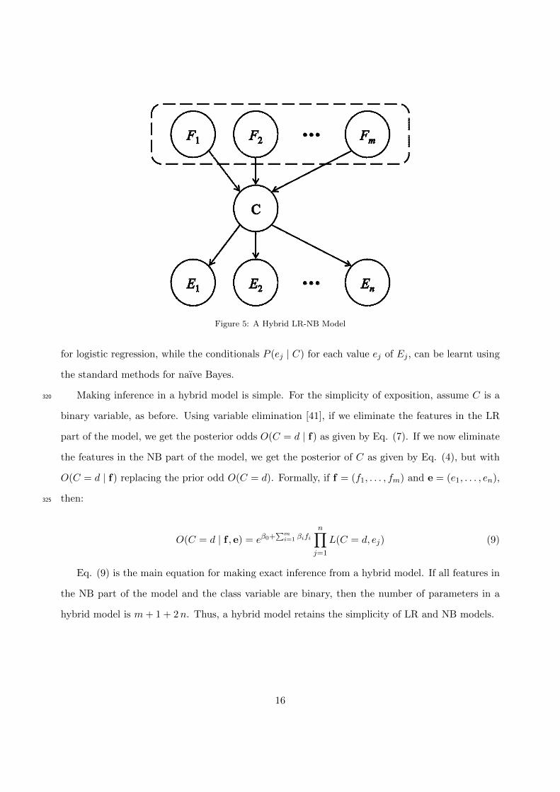
Figure 5: A Hybrid LR-NB Model
for logistic regression, while the conditionals P (ej | C) for each value ej of Ej , can be learnt using
the standard methods for naıve Bayes.
Making inference in a hybrid model is simple. For the simplicity of exposition, assume C is a320
binary variable, as before. Using variable elimination [41], if we eliminate the features in the LR
part of the model, we get the posterior odds O(C = d | f) as given by Eq. (7). If we now eliminate
the features in the NB part of the model, we get the posterior of C as given by Eq. (4), but with
O(C = d | f) replacing the prior odd O(C = d). Formally, if f = (f1, . . . , fm) and e = (e1, . . . , en),
then:325
O(C = d | f , e) = eβ0+∑m
i=1 βifi
n∏j=1
L(C = d, ej) (9)
Eq. (9) is the main equation for making exact inference from a hybrid model. If all features in
the NB part of the model and the class variable are binary, then the number of parameters in a
hybrid model is m+ 1 + 2n. Thus, a hybrid model retains the simplicity of LR and NB models.
16

8. Feature Selection and Construction of a Hybrid Model
In this section, we describe how we select features for a hybrid model, and provide an algorithm330
for the construction of hybrid model. Our method is implemented for the the 10b-5 security class-
action dataset.
Step 1: Markov Blanket Estimation. In the first step, we estimate a Markov blanket of the class
variable C. By definition, a node is conditionally independent of all other nodes given its Markov
blanket. For example, In a Bayesian network, a variable’s Markov blanket includes its parents, its335
children, and co-parents of its children. Thus, the knowledge of the features in the Markov blanket
of class C alone is sufficient to predict the class outcome. We use the training set to estimate the
Markov blanket. The Markov blanket of class variable C is estimated using learn.mb command in
bnlearn package in R [42].
Various constraint-based algorithms [43] exist in literature that use conditional independence340
tests to estimate the Markov blanket. These algorithms compute the Markov blanket directly,
without first estimating a graphical model. We use 4 different constraint-based algorithms: (i)
grow shrink [44]; (ii) incremental association [45]; (iii) fast incremental association [46]; and (iv)
interleaved incremental association [45], and 10 different conditional independence tests8 as imple-
mented in bnlearn package for each of these algorithms, resulting in 40 estimates of Markov blanket.345
We take the union of features in all 40 estimated Markov blankets as the estimated Markov blanket
of C. The logic is that a feature is excluded if all estimated 40 Markov blankets are unanimous on
the exclusion of the feature. This is only one step in feature selection.
The test results show that the estimated Markov blanket of class C contains 6 features: (i) GP ,
(ii) RF , (iii) IC, (iv) S11, (v) BR, and (vi) STD. Thus, given the values of these six features, the350
remaining three features, SI, II, and IS, are irrelevant to the class variable, subject to estimation
errors. As we have no missing values in our dataset, we proceed with these 6 features for subsequent
model selection and validation exercise.
8These conditional independence tests are for discrete variables and include asymptotic chi-square tests based onmutual information with and without adjusted degrees of freedom, Monte Carlo permutation test, the sequentialMonte Carlo permutation test, the semi-parametric test, shrinkage estimator for the mutual information, classicPearson’s chi-square test for contingency tables with and without adjusted degrees of freedom, the Monte Carloversion of the chi-square test, and the semi-parametric version of the chi-square test.
17

FR
EQ
UE
NC
Y
SHORT TERM DROP
" Not Dismissed'
"Dismissed"
42.2 %
Figure 6: Discretization of Short Term Drop
Step 2: Discretization of Continuous Features. Discretization of a continuous feature is needed only
when it is used in the NB part of the hybrid model. [47] presents an extensive survey of various355
discretization techniques. In particular, multi-level discretization technique by [48] and entropy
and MDL based discretization techniques by [49] are very useful. In this paper, we discretize STD
into two bins with cutoff value of 42.2% (i.e., STD = 0 if drop is ≤ 42.2% and 1 otherwise) .
This cut-off percentage is arrived at by supervised discretization. One effective way to discretize
a continuous feature is to look for specific breakpoints at which the class outcomes are sensitive360
to the changes in the value of a numeric feature. This implies the proportion of success to failure
(likelihood ratio) changes below and above this breakpoint. However, it is not necessary always for
such a distinct breakpoint to exist. In such cases, other discretization techniques will work. In our
dataset, we observe that ratio of frequency of dismissed to not dismissed exhibits a change around
42.2% (see Figure 6).365
Step 3: Searching for Best LR and Best NB Models. With 6 features in hand from Step 1, our goal
is to find the best LR and best NB models. By best, we mean lowest RMSE using cross validation.
If the number of features is small, we can do a complete enumeration, which involves searching
among 2q1 − 1 models, where q1 is the number of features remaining after step 1. If the number of
18

features is large, we can resort to using a forward, backward, stepwise, or random search. In our370
case, we examine (26 − 1) = 63 different subsets to find the best model.
At this juncture, we emphasize the choice of RMSE as a performance metric. Most of the
earlier works in machine learning literatures (see [26, 27]) focus on classification. Consequently,
classification error, which measures the ratio of # incorrect classifications to # total instances, is
their choice for a performance measure. However, our objective is not classification, but predicting375
the probability of dismissal. Given this objective, RMSE is a better performance metric. For
example, classification error does not distinguish between two instances having predicted posterior
probability 0.51 and 1.00, and classifies both of them as dismissed. In contrast, RMSE detects
the quantitative difference exactly. Hence, we use RMSE as the metric for model evaluation.
For each of the 63 subsets of features, we use 8-fold cross-validation (CV) on the training set380
to compute the RMSE of a model. This means we randomly partition the training set into 8 equal
parts (called folds), use 7 out of 8 folds to learn parameters and use the 8th fold (holdout set) for
validation. This is repeated 8 times with each fold as the holdout fold. At the end of the 8-fold
CV, we have estimates of predicted probability of dismissal for all 832 instances in the training
set. In the next step, we compute the RMSE of a model as described in Step 4.385
Step 4: Estimating RMSE of a Model. In order to compute RMSE, first we sort the cases by
increasing order of predicted probability of dismissal, and then partition the training set into
8 equal-sized bins (the first 104 sorted cases constitute the first bin, the next 104 sorted cases
constitute the second bin, and so on.). The choice of # bins is critical and we explain this in more
detail later. For each bin, we compute (i) the average of the predicted probabilities of dismissal,390
and (ii) the actual probability of dismissal, which is the ratio of actual # dismissed cases divided by
total number of cases in the bin. The difference between the predicted probability and the actual
probability is defined as the prediction error for each bin. We compute the sum of the squared
prediction errors for all 8 bins, divide the sum by 8 to obtain mean square error, and then take the
square root of the mean square error, which constitutes the RMSE for the entire training set. We395
repeat the process of 8-fold cross validation and computation of RMSE 100 times using different
random splits of the training data. Finally, we compute the average RMSE and the standard error
19

Table 1: A Typical example of computation of bin probability and RMSE
Avg. predicted prob. Actual prob. Sq. error
Bin 1 0.270 0.288 0.0003Bin 2 0.320 0.355 0.0012Bin 3 0.340 0.336 0.0000Bin 4 0.385 0.365 0.0004Bin 5 0.438 0.442 0.0000Bin 6 0.482 0.432 0.0024Bin 7 0.598 0.644 0.0021Bin 8 0.654 0.625 0.0008Sum of squared errors 0.0072RMSE 0.0300
of the average RMSE. We do this for all models, and choose a model having the lowest error. A
typical example of computation of predicted and true average probability and RMSE is presented
in Table 1, and is shown in Figure 7.400
Bins-Bias Trade-off. The choice of # bins (say k, k = 8 in our case) is critical for model selection.
It may be seen that the choice of k not only affects the magnitude of the RMSE of each model,
but also affects their ranking. To explain this phenomenon, we have examined RMSE of all 63 LR
models with 8-fold CV and two different bin sizes: k = 4 (see Figure 8) and k = 8 (see Figure 9).
The results show that choice of k gives rise to systemic bias towards selecting models with fewer405
features when k = 4, and models with more features when k = 8, as can be seen from Figures
8 and 9. In these two figures, the first 6 models have 1 feature, the next 13 have two features,
etc. For the case of 4-bins (Figure 8), the smallest RMSE is achieved by a model with 2 features
(model #7), whereas for the case of 8-bins (Figure 9), the smallest RMSE is achieved by a model
with 5 features (model #58). The dotted line in Figure 8 and Figure 9 represents # features in410
the model.
To explain why this bias occurs, if k denotes the number of bins of the training set, the true
probability of dismissal of the k bins can be characterized by (k − 1) parameters (assuming that
the # dismissed cases in the training set is known). When we search for models to estimate the
true probabilities of dismissal of k bins by minimizing RMSE, assuming that each binary feature415
20
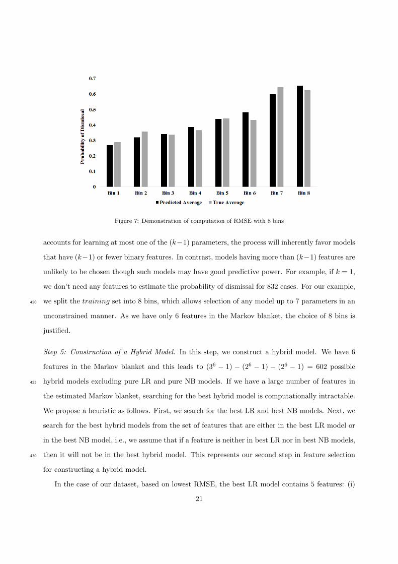
Figure 7: Demonstration of computation of RMSE with 8 bins
accounts for learning at most one of the (k−1) parameters, the process will inherently favor models
that have (k−1) or fewer binary features. In contrast, models having more than (k−1) features are
unlikely to be chosen though such models may have good predictive power. For example, if k = 1,
we don’t need any features to estimate the probability of dismissal for 832 cases. For our example,
we split the training set into 8 bins, which allows selection of any model up to 7 parameters in an420
unconstrained manner. As we have only 6 features in the Markov blanket, the choice of 8 bins is
justified.
Step 5: Construction of a Hybrid Model. In this step, we construct a hybrid model. We have 6
features in the Markov blanket and this leads to (36 − 1) − (26 − 1) − (26 − 1) = 602 possible
hybrid models excluding pure LR and pure NB models. If we have a large number of features in425
the estimated Markov blanket, searching for the best hybrid model is computationally intractable.
We propose a heuristic as follows. First, we search for the best LR and best NB models. Next, we
search for the best hybrid models from the set of features that are either in the best LR model or
in the best NB model, i.e., we assume that if a feature is neither in best LR nor in best NB models,
then it will not be in the best hybrid model. This represents our second step in feature selection430
for constructing a hybrid model.
In the case of our dataset, based on lowest RMSE, the best LR model contains 5 features: (i)
21
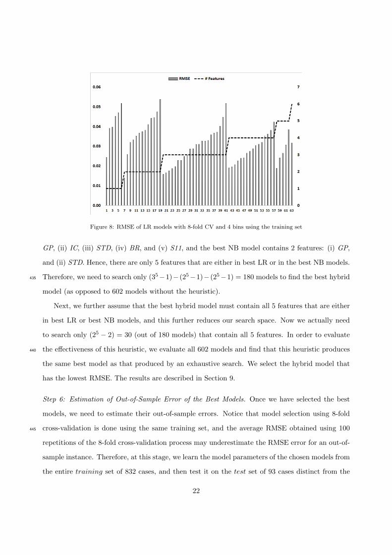
Figure 8: RMSE of LR models with 8-fold CV and 4 bins using the training set
GP, (ii) IC, (iii) STD, (iv) BR, and (v) S11, and the best NB model contains 2 features: (i) GP,
and (ii) STD. Hence, there are only 5 features that are either in best LR or in the best NB models.
Therefore, we need to search only (35−1)− (25−1)− (25−1) = 180 models to find the best hybrid435
model (as opposed to 602 models without the heuristic).
Next, we further assume that the best hybrid model must contain all 5 features that are either
in best LR or best NB models, and this further reduces our search space. Now we actually need
to search only (25 − 2) = 30 (out of 180 models) that contain all 5 features. In order to evaluate
the effectiveness of this heuristic, we evaluate all 602 models and find that this heuristic produces440
the same best model as that produced by an exhaustive search. We select the hybrid model that
has the lowest RMSE. The results are described in Section 9.
Step 6: Estimation of Out-of-Sample Error of the Best Models. Once we have selected the best
models, we need to estimate their out-of-sample errors. Notice that model selection using 8-fold
cross-validation is done using the same training set, and the average RMSE obtained using 100445
repetitions of the 8-fold cross-validation process may underestimate the RMSE error for an out-of-
sample instance. Therefore, at this stage, we learn the model parameters of the chosen models from
the entire training set of 832 cases, and then test it on the test set of 93 cases distinct from the
22
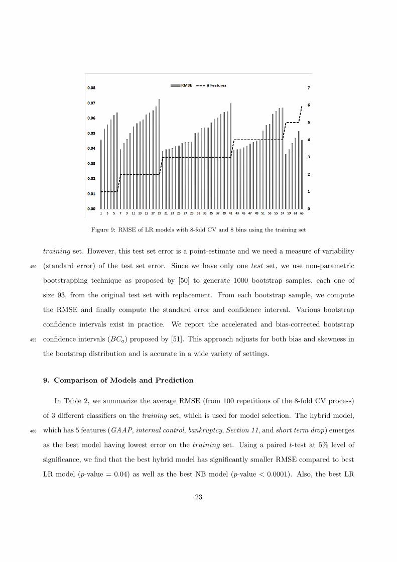
Figure 9: RMSE of LR models with 8-fold CV and 8 bins using the training set
training set. However, this test set error is a point-estimate and we need a measure of variability
(standard error) of the test set error. Since we have only one test set, we use non-parametric450
bootstrapping technique as proposed by [50] to generate 1000 bootstrap samples, each one of
size 93, from the original test set with replacement. From each bootstrap sample, we compute
the RMSE and finally compute the standard error and confidence interval. Various bootstrap
confidence intervals exist in practice. We report the accelerated and bias-corrected bootstrap
confidence intervals (BCa) proposed by [51]. This approach adjusts for both bias and skewness in455
the bootstrap distribution and is accurate in a wide variety of settings.
9. Comparison of Models and Prediction
In Table 2, we summarize the average RMSE (from 100 repetitions of the 8-fold CV process)
of 3 different classifiers on the training set, which is used for model selection. The hybrid model,
which has 5 features (GAAP, internal control, bankruptcy, Section 11, and short term drop) emerges460
as the best model having lowest error on the training set. Using a paired t-test at 5% level of
significance, we find that the best hybrid model has significantly smaller RMSE compared to best
LR model (p-value = 0.04) as well as the best NB model (p-value < 0.0001). Also, the best LR
23

Figure 10: Reliability Diagram of the Best Hybrid Model Using Data in the Training Set
Table 2: Best Models Selected and Their Average RMSE
Method # features features Avg. RMSE Std. Error
Naıve Bayes 2 GP, STD 0.0488 0.0012Logistic Regression 5 GP, IC, STD, BR, S11 0.0436 0.0010Hybrid 5 LR part : GP, IC, BR, S11 0.0412 0.0011
NB part : STD
model is found to be significantly better than the best NB model (p-value is < 0.0002) with regard
to training set error.465
We test the prediction performance of this model on the test set to represent the true error
that we might expect on a new dataset. As mentioned above, we resort to bootstrapping (1000
resamples) to estimate the standard error. The test set error of the best hybrid model, along with
standard error and confidence interval are given in Table 3. In addition, we use the reliability
diagram (see Figure 10) and the bar-chart (see Figure 11) to descriptively evaluate the model470
performance. It can be seen that the best hybrid model is well-calibrated [52].
24

Figure 11: Prediction Performance of the Best Hybrid Model Using Data in the Training Set
Table 3: Test set RMSE
Method Avg. RMSE Bootstrap Std. Error Bootstrap CI
Best Hybrid Model 0.0930 0.0444 [0.0110, 0.1843]
10. An Example
To find the parameters of a LR model, we used glm() command in stats package in R, which
is used for fitting generalized linear models. To find the parameters of a NB model, we used
naive.bayes() command in bnlearn package. To find the parameters of a hybrid model, we used475
the respective packages for the LR and NB part and then combined them using Eq. (9).
Once the best model is chosen, the parameter estimates of the best hybrid model has been
obtained using all 925 cases in our dataset. They are as follows: β0 = 0.6305, β1 = −0.3412,
β2 = −0.2507, β3 = −1.1506, β4 = −0.8105, and the likelihood ratios are L(dismissal, std =
1) = 0.6465, and L(dismissal, std = 0) = 1.097. Eq. (10) represents the probability model for480
predicting the odds of dismissal. We now demonstrate the use of our model using an example,
25
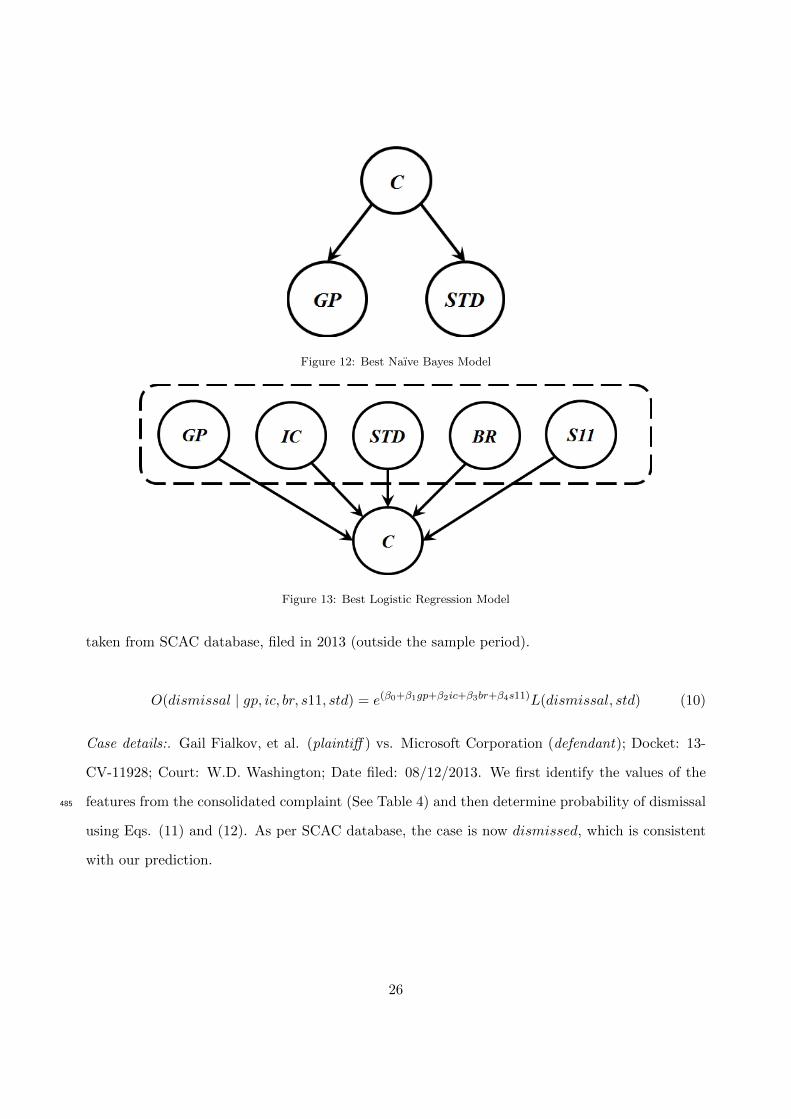
Figure 12: Best Naıve Bayes Model
Figure 13: Best Logistic Regression Model
taken from SCAC database, filed in 2013 (outside the sample period).
O(dismissal | gp, ic, br, s11, std) = e(β0+β1gp+β2ic+β3br+β4s11)L(dismissal, std) (10)
Case details:. Gail Fialkov, et al. (plaintiff ) vs. Microsoft Corporation (defendant); Docket: 13-
CV-11928; Court: W.D. Washington; Date filed: 08/12/2013. We first identify the values of the
features from the consolidated complaint (See Table 4) and then determine probability of dismissal485
using Eqs. (11) and (12). As per SCAC database, the case is now dismissed, which is consistent
with our prediction.
26

Figure 14: Best Hybrid Model
O(dismissal | gp = 1, ic = 1, br = 0, s11 = 0, std = 0)
= e(0.63+(−0.34)×1+(−0.25)×1+(−1.15)×0+(−0.81)×0)(1.09) = 1.14 (11)
P (dismissal) =O(dismissal)
O(dismissal) + 1
= 0.5327 (12)
11. Summary & Conclusions
The main contribution of this paper is a model for computing probabilities for dismissal of 10b-5
securities class-action cases filed in Federal district courts. Using a hybrid model, which combines490
logistic regression and naıve Bayes, we suggest that only 5 features are significant for predicting
the probability of (initial) dismissal. They are GAAP, internal control, bankruptcy, Section 11,
and short term drop. Only short term drop, which was discretized into 2 bins with 42.2% drop as
a cutoff value, was used in the NB part.
27

Table 4: Determining the value of the features from the consolidated complaint
[13] uses logistic regression in a Bayesian hierarchical setting to predict the probability of495
settlement/dismissal. As we mentioned earlier, the approximate training set and test set errors
were estimated from reliability diagram as 6.01% and 11.17% respectively. We show that our hybrid
model has a training set RMSE of 4.12% and a test set RMSE of 9.30%, which is an improvement
over the results in [13]. Our model is also simpler and uses only 5 features, compared to 18
features used by [13] in their model, and yet produces lower errors. Our model is designed only500
for predicting dismissal/non-dismissal, whereas the model described in [13] is a composite model
for dismissal/non-dismissal and level of settlements conditioned on non-dismissal. We believe that
feature selection using Markov blanket of dismissal helps to eliminate redundant/irrelevant features
(for dismissal) and improves prediction of probability of dismissal.
In our model, the parameter estimates (the slope coefficients) β1 through β4 are negative. This505
implies that allegation of GAAP violations, lack of internal control, violations of Section 11 of
Securities Act 1933, and bankruptcy filing by defendant, all make a class-action case less likely
to be dismissed. Our results are in agreement with the key findings in existing literatures. For
example, [33], [34] and [13], and all suggest that class-action cases with GAAP violations are less
likely to be dismissed, which is consistent with our results. Further, our finding concurs with [13]510
that violations of section 11 makes a case less prone to dismissal. However unlike us, they do not
28

find the effect statistically significant.
Our findings also complement the existing literatures, which study the determinants of set-
tlement size. For example, our results suggest that when the defendant firms file for bankruptcy
during the class period, the court is less likely to dismiss the case. However, once the case is settled,515
bankruptcy does not seem to play any role in determining the settlement size [31]. Likewise, [31]
shows that presence of institutional lead plaintiff increases the overall settlement size. In this pa-
per, we bring interesting insights by suggesting that the presence of an institutional lead plaintiff,
however, does not increase the chance of dismissal.
We do not find insider selling as a significant feature and our result concurs with [32] and [34].520
[34] explains that insider selling (a.k.a insider trading) is a commonly pleaded motive for fraud
in many complaints and are pleaded more often when stock options is a form of compensation for
employees. As a result, the courts are skeptical about this allegation.
However, unlike [32], we do not find restated financials as a significant feature. Generally,
restated financials is perceived as direct evidence for accounting violations and makes a suit less525
likely to be dismissed. In our findings, models that include GAAP violations but not restated
financials predict better than those that include both GAAP and restated financials. It is possible
that these two features are highly correlated, and including both features results in double counting
that lowers the accuracies of the models.
Further, we also observe that the short-term-drop (STD) in share price within a period of 1−5530
days is an important attribute. This agrees with our belief that STD measures the immediate
impact of the security fraud and is a proxy of the financial loss suffered by investors. Hence, we
expect the likelihood of dismissal to be lower when share price drop is > 42.2%. In our case, the
likelihood ratio for dismissal is 0.6465 when STD > 42.2% and 1.097 when STD ≤ 42.2%, which
includes no allegation of short term drop in the consolidated complaint (see Section 10). Thus, an535
allegation of STD > 42.2% favors non-dismissal, which is consistent with our belief.
Finally, our model suggests that an allegation of lack of internal control is an important feature
for predicting probability of dismissal. This feature has not been widely studied in the past.
However, lack of internal control is being increasingly alleged in security class-actions. On an
29

average, 23% of all class-actions filed during 2011–2015 have alleged internal control weaknesses540
over financial reporting [35]. Hence, lack of internal control is an important feature for predicting
dismissal.
In conclusion, we present a model that can be used to predict probability of dismissal in response
to motion to dismiss. The model identifies 5 features that are significant for predicting dismissal,
and largely consistent with the existing literature. The proposed hybrid model for computation of545
probability of dismissal will act a decision support tool for the D&O insurers in U.S. Since virtually
every public corporations in U.S. buy D&O insurance, there is an increasing interest in predicting
the probability of dismissal of class-action cases. Even knowing what features are relevant for
predicting probabilities of dismissal is also useful for assessment of underwriting risks for D&O
insurance. Considering the size of class-action settlements and increasing incidence of class-action550
cases, we believe that an improvement in predictive performance will go a long way.
Acknowledgement
This project was funded in part by a sponsored research project from a D&O insurance com-
pany (which wishes to remain anonymous) to the Center for Business Analytics Research, School
of Business, University of Kansas. We are grateful to the global head of the D&O company (un-555
named for anonymity reasons) for helping us with classifying cases in our dataset as dismissed/not
dismissed. Thanks to Suzanna Emelio at University of Kansas for proofreading this manuscript.
References
[1] M. Mora, O. Gelman, G. Forgionne, F. Cervantes, The implementation of large-scale decision-making support
systems: Problems, findings, and challenges, Encyclopedia of Decision Making and Decision Support Technolo-560
gies 2 (2008) 455.
[2] R. H. Sprague Jr, E. D. Carlson, Building effective decision support systems, Prentice Hall Professional Technical
Reference, 1982.
[3] M. Amann, M. Makowski, Effect-focused air quality management, Mathematical Modeling Theory and Appli-
cations 9 (2000) 367–398.565
[4] S. Strubegger, M. Messner, Model–based decision support in energy planning, International Journal of Global
Energy Issues 12 (1-6) (1999) 196–207.
30
[5] F. Ghasemzadeh, N. P. Archer, Project portfolio selection through decision support, Decision Support Systems
29 (1) (2000) 73–88.
[6] L. Bai, J. D. Cox, R. S. Thomas, Lying and getting caught: An empirical study of the effect of securities class570
action settlements on targeted firms, University of Pennsylvania Law Review 158 (7) (2010) 1877–1914.
[7] J. C. Coffee, Reforming the securities class action: An essay on deterrence and its implementation, Columbia
Law Review 106 (7) (2006) 1534–1586.
[8] T. Eisenberg, G. P. Miller, Attorney fees and expenses in class action settlements: 1993–2008, Journal of
Empirical Legal Studies 7 (2) (2010) 248–281.575
[9] B. T. Fitzpatrick, An empirical study of class action settlements and their fee awards, Journal of Empirical
Legal Studies 7 (4) (2010) 811–846.
[10] T. Baker, S. J. Griffith, Predicting corporate governance risk: Evidence from the directors’ and officers’ liability
insurance market, Chicago Law Review 74 (2007) 487.
[11] T. Baker, S. J. Griffith, How the merits matter: Directors’ and officers’ insurance and securities settlements,580
University of Pennsylvania Law Review 157 (3) (2009) 755–832.
[12] J. E. Core, On the corporate demand for directors’ and officers’ insurance, The Journal of Risk and Insurance
64 (1) (1997) 63–87.
[13] B. B. McShane, O. P. Watson, T. Baker, S. J. Griffith, Predicting securities fraud settlements and amounts: A
hierarchical Bayesian model of Federal securities class action lawsuits, Journal of Empirical Legal Studies 9 (3)585
(2012) 482–510.
[14] D. H. Wolpert, The supervised learning no-free-lunch theorems, in: R. Roy, M. Koppen, S. Ovaska, T. Furuhashi,
F. Hoffmann (Eds.), Soft Computing and Industry: Recent Applications, Springer, London, 2002, pp. 25–42.
[15] C. K. Chow, Statistical independence and threshold functions, IEEE Transactions on Electronic Computers
EC-14 (1) (1965) 66–68.590
[16] B. V. Dasarathy, B. V. Sheela, A composite classifier system design: concepts and methodology, Proceedings of
the IEEE 67 (5) (1979) 708–713.
[17] M. Wozniak, M. Grana, E. Corchado, A survey of multiple classifier systems as hybrid systems, Information
Fusion 16 (2014) 3–17.
[18] L. A. Rastrigin, R. H. Erenstein, Method of Collective Recognition, Energoizdat, Moscow, 1981.595
[19] R. T. Clemen, Combining forecasts: A review and annotasted bibliography, International journal of forecasting
5 (4) (1989) 559–583.
[20] K. Tumer, J. Ghosh, Analysis of decision boundaries in linearly combined neural classifiers, Pattern Recognition
29 (2) (1996) 341–348.
[21] R. Raina, Y. Shen, A. McCallum, A. Y. Ng, Classification with hybrid generative/discriminative models, in:600
S. Thrun, L. Saul, B. Scholkopf (Eds.), Advances in Neural Information Processing Systems 16, MIT Press,
2004, pp. 545–552.
31

[22] Y. D. Rubinstein, T. Hastie, Discriminative vs Informative Learning, in: Proceedings of the Third International
Conference on Knowledge Discovery and Data Mining (KDD-97), AAAI Press, 1997, pp. 49–53.
[23] G. Bouchard, B. Triggs, The tradeoff between generative and discriminative classifiers, in: J. Antoch (Ed.),605
16th International Symposium on Computational Statistics (COMPSTAT ’04), 2004, pp. 721–728.
[24] B. M. Kelm, C. Pal, A. McCallum, Combining generative and discriminative methods for pixel classification
with multi-conditional learning, in: 18th International Conference on Pattern Recognition (ICPR’06), Vol. 2,
IEEE, 2006, pp. 828–832.
[25] C. M. Bishop, J. Lasserre, et al., Generative or discriminative? Getting the best of both worlds, Bayesian610
statistics 8 (8) (2007) 3–24.
[26] C. Kang, J. Tian, A hybrid generative/discriminative Bayesian classifier, in: G. Sutcliffe, R. Goebel (Eds.),
Proceedings of the 19th International Florida Artificial Intelligence Research Society Conference (FLAIRS-06),
2006, pp. 562–567.
[27] J. H. Xue, D. M. Titterington, Joint discriminative-generative modelling based on statistical tests for classifi-615
cation, Pattern Recognition Letters 31 (9) (2010) 1048–1055.
[28] A. Y. Ng, M. I. Jordan, On discriminative vs. generative classifiers: A comparison of logistic regression and
naıve Bayes, in: T. G. Dietterich, S. Becker, Z. Ghahramani (Eds.), Advances in Neural Information Processing
Systems 14, MIT Press, 2002, pp. 841–848.
[29] J. H. Xue, D. M. Titterington, On the generative–discriminative tradeoff approach: Interpretation, asymptotic620
efficiency and classification performance, Computational Statistics & Data Analysis 54 (2) (2010) 438–451.
[30] J. D. Cox, R. S. Thomas, D. Kiku, Does the plaintiff matter? An empirical analysis of lead plaintiffs in securities
class actions, Columbia Law Review 106 (7) (2006) 1587–1640.
[31] J. D. Cox, R. S. Thomas, L. Bai, There are plaintiffs and there are plaintiffs: An empirical analysis of securities
class action settlements, Vanderbilt Law Review 61 (2) (2008) 355–386.625
[32] M. F. Johnson, K. K. Nelson, A. C. Pritchard, Do the merits matter more? The impact of the Private Securities
Litigation Reform Act, Journal of Law, Economics, and Organization 23 (3) (2007) 627–652.
[33] M. Klausner, J. Hegland, When are securities class actions dismissed, when do they settle, and for how much?,
Plus Journal 23 (3) (2010) 1–5.
[34] A. C. Pritchard, H. A. Sale, What counts as fraud? An empirical study of motions to dismiss under the Private630
Securities Litigation Reform Act, Journal of Empirical Legal Studies 2 (1) (2005) 125–149.
[35] A. Aganin, Securities class action filings—2015 year in review, Research report, Cornerstone Research, Inc.
(2016).
[36] D. Koller, M. Sahami, Toward optimal feature selection, Technical Report 1996-77, Stanford InfoLab (February
1996).635
[37] S. Fu, M. C. Desmarais, Markov blanket based feature selection: A review of past decade, in: Proceedings of
the World Congress on Engineering, Vol. 1, 2010, pp. 321–328.
32

[38] S. Hillmer, P. P. Shenoy, Computing the probabilities of closing of 10b-5 securities class action cases, http:
//pshenoy.faculty.ku.edu/BUS936/Powerpoint/ShenoySp14.pdf, available Online; January 31, 2014 (2014).
[39] P. Domingos, M. Pazzani, On the optimality of the simple Bayesian classifier under zero-one loss, Machine640
Learning 29 (2–3) (1997) 103–130.
[40] A. P. Dempster, N. M. Laird, D. B. Rubin, Maximum likelihood from incomplete data via the EM algorithm,
Journal of the Royal Statistical Society, Series B 39 (1) (1977) 1–38.
[41] N. L. Zhang, D. Poole, A simple approach to Bayesian network computations, in: Proceedings of the 10th
Canadian Conference on Artificial Intelligence, Springer, NY, 1994, pp. 171–178.645
[42] M. Scutari, J. B. Denis, Bayesian networks: with examples in R, CRC Press, 2014.
[43] J. Pearl, Probabilistic Reasoning in Intelligent Systems: Networks of Plausible Inference, Morgan Kaufmann,
2014.
[44] D. Margaritis, Learning Bayesian network model structure from data, Ph.D. thesis, Carnegie Mellon University
School of Computer Science, Pittsburgh, PA (2003).650
[45] I. Tsamardinos, C. F. Aliferis, A. Statnikov, Algorithms for large scale Markov blanket discovery, in: Proceedings
of the Sixteenth International Florida Artificial Intelligence Research Society Conference (FLAIRS-03), 2003,
pp. 376–381.
[46] S. Yaramakala, D. Margaritis, Speculative Markov blanket discovery for optimal feature selection, in: Pro-
ceedings of the Fifth IEEE International Conference on Data Mining (ICDM-05), IEEE Computer Society,655
Washington, DC, 2005, pp. 809–812.
[47] S. Kotsiantis, D. Kanellopoulos, Discretization techniques: A recent survey, GESTS International Transactions
on Computer Science and Engineering 32 (1) (2006) 47–58.
[48] U. Fayyad, K. B. Irani, Multi-interval discretization of continuous-valued attributes for classification learning,
in: R. Bajcsy (Ed.), Proceedings of the 13th International Joint Conference on Artificial Intelligence, 1993, pp.660
1022–1029.
[49] E. J. Clarke, B. A. Barton, Entropy and MDL discretization of continuous variables for Bayesian belief networks,
International Journal of Intelligent Systems 15 (1) (2000) 61–92.
[50] B. Efron, R. Tibshirani, Bootstrap methods for standard errors, confidence intervals, and other measures of
statistical accuracy, Statistical Science 1 (1) (1986) 54–75.665
[51] B. Efron, Better bootstrap confidence intervals, Journal of the American Statistical Association 82 (397) (1987)
171–185.
[52] A. Niculescu-Mizil, R. Caruana, Predicting good probabilities with supervised learning, in: Proceedings of the
22nd International Conference on Machine Learning (ICML-05), ACM, 2005, pp. 625–632.
33


![10B-LR 10B-SUBold.bryston.com/PDF/Manuals/300001[10B].pdf · The 10B-STD and 10B-SUB crossovers generate a summed low pass output signal by first summing or adding together the left](https://static.fdocuments.us/doc/165x107/5fca308acddab466873f1279/10b-lr-10b-10bpdf-the-10b-std-and-10b-sub-crossovers-generate-a-summed-low.jpg)


![JICA 201610B 10B 10B 13B 22 10B 11B 11B 26B M2:30 JTñ-ñ-3— … · 2016-10-13 · JICA 201610B 10B 10B 13B 22 10B 11B 11B 26B M2:30 JTñ-ñ-3— JD+ñ3—] (3) @ @ @ 201 2016 11](https://static.fdocuments.us/doc/165x107/5f7b7664c26e297ff6248b8f/jica-201610b-10b-10b-13b-22-10b-11b-11b-26b-m230-jt-3a-2016-10-13-jica.jpg)