on COMPUTATIONAL ASPECTS in CONTROL FLEXIBLE SYSTEMS · 2013-08-30 · Thomas No11 and Boyd Perry...
518
NASA Technical Memorandum 10 1578, Part One WORKSHOP on COMPUTATIONAL ASPECTS in the CONTROL of FLEXIBLE SYSTEMS Held at the Royce Hotel in WiIIiamsburg, Virginia (\!~?~-~*-lolj?d-pt-l) P & ~ C ~ L ~ I N ~ Y -F THE <UL ( ; 8.; t\jo~-l?~Su ~~KY,~+~JD fl~ CnHPUTATIONAL ASPFCTI IY TcF --T )~uI)-- ~ f ' 4T1.1L dC Ei'XfrLt. >Y>TtU,, f'AQT i (.\A>A- r\eu-lP>CL L an-1-y Rps~arih Centnr) 492 p C5CL 2LR UnLl ~s 55 3 G;/i3 J,'i74qA Sponsored by the NASA Langley Research Center Proceedings Compiled by Larry Taylor https://ntrs.nasa.gov/search.jsp?R=19900000764 2020-04-28T21:36:31+00:00Z
Transcript of on COMPUTATIONAL ASPECTS in CONTROL FLEXIBLE SYSTEMS · 2013-08-30 · Thomas No11 and Boyd Perry...

NASA Technical Memorandum 10 1578, Part One
WORKSHOP on COMPUTATIONAL ASPECTS in the CONTROL of FLEXIBLE SYSTEMS
Held at the Royce Hotel in WiIIiamsburg, Virginia
( \ ! ~ ? ~ - ~ * - l o l j ? d - p t - l ) P & ~ C ~ L ~ I N ~ Y -F T H E <UL (; 8.; t \ j o ~ - l ? ~ S u ~ ~ K Y , ~ + ~ J D f l ~ CnHPUTATIONAL A S P F C T I IY TcF - - T ) ~ u I ) - -
~ f ' 4T1 .1L dC Ei'XfrLt. > Y > T t U , , f 'AQT i ( . \ A > A - r \ e u - l P > C L
L a n - 1 - y R p s ~ a r i h C e n t n r ) 4 9 2 p C 5 C L 2 L R U n L l ~s
55 3 G ; / i 3 J , ' i 7 4 q A
Sponsored b y the NASA Langley Research Center
Proceedings Compiled b y Larry Taylor
https://ntrs.nasa.gov/search.jsp?R=19900000764 2020-04-28T21:36:31+00:00Z


Table of Contents
Page
Introduction
Computational Aspects Workshop Call for Papers 1
Workshop Organizing Committee 5
Attendance List 7
--------___-----__-------------------------------------- Needs for Advanced CSI Software
NASA's Control/Structures Interaction (CSI) Program Brantley R. Hanks, NASA Langley Research Center 2 1 - ,
Computational Controls for Aerospace Systems Guy Man, Robert A. Laskin and A. Fernando Tolivar Jet Propulsion Laboratory 3 3 .
Additional Software Developments Wanted for Modeling and Control of Flexible Systems
Jiguan G. Lin, Control Research Corporation 4 9
Survey of Available Software
Flexible Structure Control Experiments Using a Real-Time Workstation for Computer-Aided Control Engineering
Michael E. Steiber, Communications Research Centre 6 7
CONSOLE: A CAD Tandem for Optimizationl-Based Design Interact ing with User-Supplied Simulators
Michael K.H. Fan, Li-Shen Wang, Jan Koninckx and Andre L. Tits,University of Maryland, College Park 8 9
m L PAGE IS QUALfTY

ORIGINAL PAGE IS OF POOR QUALITY
The Application of TSIM Software to ACT Design and Analysis of Flexible Aircraft
Ian W. Kaynes, Royal Aerospace Establishment, Farnborouth 109 - Control/Structure Interaction Methods for Space Statian Power Systems
Paul Blelloch, Structural Dynamics Research Corporation 1 2 1 L ,
Flexible Missile Autopilot Design Studies with PC-MATLAB386 Michael J. Ruth, Johns Hopkins University Applied Physics Laboratory 1 3 9
DYSCO - A Software System for Modeling General Dynamic Systems Alex Berman, Kaman Aerospace Corporation 1 6 7
Modeling and Control System Design and Analysis Tools for Flexible St ruc tures
Amir A. Anissipour and Edward E. Coleman The Boeing Company 2 2 1
Lumped Mass Formulations for Modeling Flexible Body Systems R. Rampalli, Mechanical Dynamics, Inc. 2 4 3
r I
A Comparison of Software for the Modeling and Control of Flexible Systems
Lawrence W. Taylor, Jr., NASA Langley Research Center 2 6 5
-- ---------- --- -------- Computational Efficiency and Capability
Large Angle Transient Dynamics (LATDYN) - A NASA Facility for Research in Applications and Analysis Techniques for Space Structure Dynamics
Che-Wei Chang, Chih-Chin Wu,COMTEK Jerry Housner, NASA Langley Res. Ctr. 2 8 3
Enhanced Element-Specific Modal Modal Formulations for FIexi ble Multibody Dynamics
Robert R. Ryan, University of Michigan

Efficiency and Capabilities of Multi-Body Simulations Richard J. VanderVoort, DYNACS Engineering Co., Inc. 3 4 9
Explicit Modeling and Computational Load Distribution for Concurrent Processing Simulation of the Space Station
R. Gluck, TRW Space and Technology Group 371
Simulation of Flexible Structures with Impact: Experimental Validation A. Galip Ulsoy, University of Michigan 4 1 5
Simulation and Control Problems in Elastic Robots S. S. K. Tadikonda and H. Baruh, Rutgers University 417
Linearized Flexibility Models in Multibody Dynamics and Control William W. Cimino, Boeing Aerospace 4 4 1
Simulation of Shuttle Flight Control System Structural Interaction with RMS Deployed Payloads
Joseph Turnball, C. S. Draper Laboratories 4 7 3
A Performance Comparison of Integration Algorithms in Simulating Flexible Structures
R. M. Howe, University of Michigan 4 9 5
Data Processing for Distributed Sensors in Control of Flexible S p a c e c r a f t
Sharon S. Welch, Raymond C. Montgomery, Michael F. Barsky and Ian T. Gallimore, NASA Langley Research Center 5 1 3
******* PART TWO ........................................................
Modeling and Parameter Estimation
Flexible Robot Control: Modeling and Experiments Irving J. Oppenheim, Carnegie Mellon University Isao Shimoyama, University of Tokyo 5 4 9
Minimum-Variance Reduced-Order Estimation Algorithms from Pontrygin's Minimum Principle
Yaghoob S. Ebrahimi, The Boeing Company 581
Modifying High-Order Aeroelastic Math Model of a Je t Transport Using Maximum Likelihood Estimation
Amir A. Anissipour and Russell A. Benson The Boeing Company
Automated Model Formulation for Time VArying Flexible S t r u c t u r e s
B. J. Glass, Georgia Institute of Technology 6 3 1
Numerically Efficient Algorithm for Model Development of High Order Systems
L. Parada, Calspan Advanced Technical Center 6 3 3
On Modeling Nonlinear Damping in Distributed Parameter Systems A. V. Balakrishnan, U. C. L. A. 6 5 1
Use of the Quasilinearization Algorithm for the Simulation of LSS Slewing
Peter M. Bainum and Fieyue Li, Howard University 6 6 5
.......................................................... Control Synthesis and Optimization Software
Control Law Synthesis and Optimization Software for Large O r d e r Aeroservoelastic Systems
V. Mukhopadhyay, A. Pototzky and T. No11 NASA Langley Research Center 6 9 3
Flexible Aircraft Dynamic Modeling for Dynamic Analysis and Control Synthesis
David K. Schmidt, Purdue University 7 0 9
Experimental Validation of Flexible Robot Arm Modeling and Cont ro l
A. Galip Ulsoy, University of Michigan 7 4 5
Controlling Flexible Structures - A Survey of Methods Russell A. Benson and Edward E. Coleman The Boeing Company 7 7 9

Aircraft Modal Suppression System: Existing Design Approach and I t s Shortcomings
J. Ho, T. Goslin and C. Tran, The Boeing Company 8 0 1
Structural Stability Augmentation System Design Using BODEDIRECT: A Quick and Accurate Approach
T. J. Goslin and J. K. Ho, The Boeing Company 8 2 5
Optimal q-Markov Cover for Finite Precision Implementation Darrell Williamson and Robert E. Skelton, Purdue University 853
Input-Output Oriented Computational Algorithms for the Control of Large Flexible Structures
K. Dean Minto and Ted F. Knaak, General Electric 8 8 3
The Active Flexible Wing Aeroservoelastic Wind-Tunnel Test P r o g r a m
Thomas No11 and Boyd Perry I11 NASA Langley Research Center 9 0 3
Modeling and Stabilization of Large Flexible Space Stations S. Lim and N. U. Ahmed, University of Ottawa, Canada 9 4 3
Active Vibration Mitigation of Distributed ]Parameter, Smart- Type Structures Using Pseudo-Feedback Optimal Control
W. Patten, University of Iowa; H. Robertshaw, D. Pierpont and R. Wynn, Virginia Polytechnic Institute and State University 9 5 7
Shape Control of High Degree-of-Freedon Variable Geometry T r u s s e s
R. Salerno, Babu Padmanabhan, Charles F. Reinholtz, H. Robertshaw Virginia Polytechnic Institute and State University 9 8 3
Optimal Integral Controller with Sensor Failure Accomodations Thomas Alberts, Old Dominion University Thomas Houlihan, The Jonathan Corporation 1 0 0 3
P o s t s c r i p t Lawrence W. Taylor, Jr., NASA Langley Research Center 1 0 2 5


Nal~onal Aeronaultcs and Space Adm~nislratlon
Langley Research Center Hamgton. Virginla 23665-5225
April 12, 1988
TO: Invited Workshop Participants
FROM: L-awrence W. Taylor, Jr., Chairman
SlJI3JIJ(JT: Workshop on Computational Aspects in the Control of Flexible Systems
I5A(:K(;ROUND: As aerospace vehicles and robotic systems become larger and more flexible, the attendant complexity results in an increased demand for high fidelity dynamic ni(xlels. This in turn can cause an excessive computational burden for model development, systems analysis and real-time simulation.
A n u ~ n k r of software packages are available for modeling flexible structures and for control anirlysis, but there remain unsatisfied needs for more efficient and more comprehensive software which is easy to use for modeling, analysis, synthesis and simulation. Low cost p;rr;illcl prtxessing promises significant increases in computational speed.
(;OAL: To assess the state of the technology in software tools for simulation analysis and synthesis for the control of flexible aerospace systems; establish capabilities and performance o f tlicse tools when applied to specific example problems; and to identify gaps and shortcomings of software tools.
AI'l'KOACIi: A workshop will be held at the Royce Hotel in Williamsburg, Virginia, July 12-14 , 1988. This workshop is being organized under the auspices of the Office of Aeronautics iind Space Technology (OAST) in NASA Headquarters, and is being chaired by the following people:
I,a~vrcnce W. Taylor, Jr. Virginia B. Marks NASA 1,angley Research Center NASA Langley Research Center M / S 489 M/S 479 I l;~nipton, V A 23665-5225 Hampton, VA 23665-5225 (%04)X65-37 16 (804)865-2077
Present;rtions and demonstrations will be given as requested in the Call for Papers (below). 111 addition, a piinel of experts will be assembled to summarize workshop presentations, lead a ciiscussion o n the state of the technology concerning computational aspects in the control of flexible struc~ures and reconirnend future direction of research and areas of concentration. A procccdings will be published and distributed following the workshop which will include presentation m;rterials with brief explanations and an address list of workshop attendees.

CALL FOR PAPERS: Presentations will be scheduled for 30 minute time slots including a period for questions and answers. We encourage submissions of one-page abstracts of proposed presentations for the following categories:
MODELING SOFTWARE FOR FLEXIBLE STRUCTURES: Special model formulations, inodel building, model reduction, modeling articulated, flexible structures.
SYSTEMS ANALYSIS AND SYNTHESIS SOFTWARE: Control synthesis, time-varying system analysis, and nonlinear system analysis
ROBOTIC SYSTEMS APPLICATIONS: Modeling experiences, needed software advances, comparison simulation and actual experience.
SPACECRAFT APPLICATIONS: Comparisons of actual and expected system stability and performance, integrated design techniques.
AIRCRAFT APPLICATIONS: Techniques by which flexibility is treated, capabilities of high fidelity simulation, comparison between actual and expected flight system stability and performance.
SIMULATION COMPUTERS: Workstations for analysis and synthesis, parallel processing for simulation.
SOFTWAREIOOMPUTER DEMONSTRATIONS: Software developers and vendors are encouraged to demonstrate the capabilities of their wares. Sun and Microvax workstations will be available and space will be provided for additional equipment and displays. For details call Larry Taylor, (804)865-3716.
PARTICIPATION: Attendance at this conference by nonpresenters is also encouraged to f~cilitate thorough discussions in all areas. Special arrangements are not required for non- U.S. citizens attending the workshop in Williamsburg. However, if a non-U.S. citizen desires access to the Langley Research Center for any reason, a letter of endorsement from your Embassy in Washington, DC, must be forwarded to NASA Headquarters before plans can be armnged. The address is:
National Aeronautics and Space Administration International Affairs Division Code XIC Washington, DC 10536-001
RESERVATIONS: A block of rooms has been reserved at the Royce Hotel for attendees of the Workshop on Computational Aspects in the Control of Flexible Systems. The special room rates for this workshop are:
TYKS of Room Bills
Single $60.00 + 6.5% tax Double $70.00 + 6.5% tax
The cut-off date for these rooms is June 11, 1988. Reservations requested beyond the cut-off date are subject to availability. Rooms may be available after this date, but not necessarily at the same rate. To make reservations, call (804)229-4020 and request a room reserved for the Workshop on Computational Aspects in the Connol of Flexible Systems or return the

enclosed reservation form before the cut-off date. Reservations must be arranged by the individual attendees, keeping in mind that during the summer Colonial Williamsburg is a popular vacation site.
HF:(;ISTRATION: A registration form for the workshop is enclosed. Please complete this form and return it by June 1 1, 1988.
DEADLINES: All submissions must be accompanied by the title, full name, affiliation, complete address and telephone number of each co-author in regular sessions and each participant in panel sessions.
M A Y 1, 1988: Indicate interest in demonstrating software packages or computers by calling Larry Taylor, Chairman.
JUNE 1, 1988: Submit one-page abstract for proposed technical presentations to Gin Marks, Vice Chairman.
JUNE 1 1, 1988: Registration forms due to Gin Marks. Cut-off date for reservations at the Royce Hotel at the special group rate.
J U N E 22, 1988: Authors are notified of presentation acceptance. Demonstrators are notified on demonstration acceptance.
J U L Y 1, 1988: Finalized agenda is sent to all registered atttendees.
JULY 12, 1988: First day of workshop. Authors are asked to provide camera ready copies of presentation material with brief explanations included for workshop proceedings.
Early response to the Call for Papers and submission of your registration forms is appreciated a successful workshop.
Lawrence W. Taylor, Jr. Chairman
Er~closures: P~liminary Agenda Kegisrration Form Reservation Request L x ~ r t l Atuactions Golf 1:acilities "Willianlsburg Great Entertainer"

COMPUTATIONAL ASPECTS WORKSHOP ORGANIZATION
Chairman
Admini s tra tor
Aero Program Chairman
Robotics Program Chairman
Space Program Chairman
Computational Facilities Coord.
Meeting Site Contract Coord.
Mail List Secretary
Proceedings Compiler
Consul tant
Larry Taylor
Trish Johnson
Jerry Elliott
Jack Pennington
Jerry Newsom
George Tan
Pat Gates
Trish Johnson
Larry Taylor
Gin Marks
PRECEDING PAGE BLANK NOT FILMED
~ & G c T I ~ ~ ~ gum

Attendance List for the
WORKSHOP ON
COMPUTATIONAL ASPECTS
IN THE CONTROL OF FLEXIBLE SYSTEMS
JULY 12-14, 1988
ROYCE HOTEL, EMPIRE BALLROOM
WILLIAMSBURG, VIRGINIA
pRECEOlNG PAGE BLANK NOT FILMED

Dr. Willard w. Anderson NASA Langley Research Center Mail Stop 479 Hampton, VA 23665-5225 804-865-3049
Dr. Ernest S. Armstrong NASA Langley Research Center Mail Stop 499 Hampton, VA 23665-5225 804-865-4848
Prof. A. V. Balakrishnan University of California at LA School of Eng. and Applied Science 6731 Boelter Hall Los Angeles, CA 90024-1600 213-825-2180
W. Keith Belvin NASA Lanqley Research Center Mail Stop 499 Hampton, VA 23665-5225 804-865-3801
Dr. Douglas Bernard Jet Propulsion Laboratory Mail Code 198-326 4800 Oak Grove Drive Pasadena, CA 91109 818-354-2597
Dr. Paul Blelloch Structural Dynamics Research Corp. 11055 Roselle Street San Diego, CA 92121-1276 619-450-1553
John Butwin Hughes Aircraft - Space & Comm Grp P.O. Box 92919 Los Angeles, CA 90009 213-606-1787
C. W. Chang COMTEK 305 Susan Newton Lane Tabb, VA 23602
Amir A. Anissipour The Boeing Company P.O. BOX 3707, M/S 9W-38 Seattle, WA 98124-2207 206-277-4390
Peter M. Bainum Howard University Dept. of Mechanical Engineering Washington, DC 20059 202-636-6612
Michael Barsky NASA Langley Research Center Mail Stop 161 Hampton, VA 23665-5225 804-865-4591
Alex Berman Kaman Aerospace Corporation D-435, Building 2 P.O. Box 2 Bloomfield, CT 06002-0002 203-243-7215
Dr. Saroj K. Biswas Temple University Dept of Electrical Engineering Philadelphia, PA 19122 215-787-8403
Kerman Buhariwala Spar Aerospace Limited 1700 Ormont Drive Weston, Ontario M9L 2W7 CANADA 416-745-9680 X4
John E. Byrne Aastra Aerospace 1685 Flint Road Dcwnsview, Ontario M3J-2W8 CANADA 416-736-7070
~haur-Ming Chou University of Lowell Dept of Mechanical Engineering Lowell, MA 01854

Prof. Ajit K. Choudhury Howard University Dept of Electrical Engineering Washington, DC 20059 202-636-7124
William W. Cimino Boeing Aerospace P.O. Box 3999 Mail Stop 82-24 Seattle, WA 98124 206-773-5191
William Clark Edward E. Coleman VPI&SU The Boeing Company Mechanical Engineering Department P.O. Box 3707, M / S 9W-38 Randolph Hall Seattle, WA 98124-2207 Blacksburg, VA 24061 206-277-3189 703-961-7038
John B. Dahlgren Jet Propulsion Laboratory ail Stop 198-330 4800 Oak Grove Drive Pasadena, CA 91109 818-842-2039
Dr. Yaghoob S. Ebrahimi The Boeing Company P.O. Box 3707, M/S 9W-38 Seattle, WA 98124-2207 206-277-2261
KO-Hui M . Fan University'of Maryland Systems Research Center College Park, MD 20742 301-454-8832
Ian T. Gallimore NASA Langley Research Center Mail Stop 161 Hampton, VA 23665-5225 804-865-4591
Michael G. Gilbert NASA Langley Research Center Mail Stop 243 Hampton, VA 23665-5225 804-865-2388
Dr. Arthur R. Dusto Boeing Advanced Systems P.O. Box 3707 M/S 33-12 Seattle, WA 98124-2207 206-241-4393
Dr. John W. Edwards NASA Langley Research Center Mail Stop 173 Hampton, VA 23665-5225 804-865-4236
Shalom Fisher Naval Research Laboratory Code 8241 4555 Overlook Avenue, S.W. Washington, DC 20375-5000
Dave Ghosh NASA Langley Research Center (FRC) Mail Stop 161 Hampton, VA 23665-5225 804-865-4591
Rafael Gluck TRW Inc. - Space Technology Group R4/1408 One Space Park Redondo Beach, CA 90278 213-297-3655
Dr. Nesim Halyo Prof. S. Hanagud Information & Control Systems, Inc. George Institute of Technoloqy 28 Research Drive School of Aerospace Engineerrng Hampton, VA 23666 Atlanta, GA 30332 804-865-0371 404-894-3000
PRECEDING PAGE BLANK NOT FILMED

Brantley R. Hanks NASA Langley Research Center Mail Stop 161 Hampton, VA 23665-5225 804-868-3058
Garnett C. Horner NASA Langley Research Center Mail Stop 230 Hampton, VA 23665-5225 804-865-3699
Dr. Jerrold M. Housner NASA Langley Research Center Mail Stop 230 Hampton, VA 23665-5225 804-865-4423
Glenda L. Jeffrey NASA Langley Research Center Mail Stop 230 Hampton, VA 23665-5225 804-865-4513
Dr. Suresh M. Joshi NASA Langley Research Center MS 161 Hampton, VA 23665-5225 804-865-4591
Prof. Walter Karplus University of California at LA School of Eng. and Applied Sciences 3732B Boelter Hall Los Angeles, CA 90024 213-825-2929
Ian W. Kaynes Royal Aircraft Establishment M&S Department, X33 Farnborough Hampshire GU146TD ENGLAND 0252-24461x5591
Robert A. Laskin Jet Propulsion Laboratory Attn: 198-326/Robert A. Laskin Mail Stop 198-326 4800 Oak Grove Drive Pasadena, CA 91109 818-354-5086
Dr. George R. Hennig The Boeing Company P.O. Box 3707, M/S 9W-38 Seattle, WA 98124-2207 206-277-4273
Dr. T. Houlihan The Jonathan Corporation 150 Boush Street Norfolk, VA 23510 804-640-7140
Robert Howe Applied Dynamics International 3800 Stone School Road Ann Arbor, MI 48108 313-973-1300
Dexter Johnson NASA Langley Research Center Mail Stop 230 Hampton, VA 23665-5225 804-865-2738
Dr. Dinesh S. Joshi Northrop Aircraft Division Dept. 3836/82 One Northrop Avenue Hawthorne, CA 90250-3277 213-332-7808
David S. Kawg Charles Stark Draper Laboratory Mail Stop 4C 555 Technology Square Cambridge, MA 02139
Ted F. Knaak General Electric Valley Forge Space Center Box 8555, Bldg 100, Room U4248 Philadelphia, PA 19101 215-354-3672
Danette Lenox NASA Langley Research Center (PRC) Mail Stop 161 Hampton, VA 23665-5225 804-865-4591

Feiyue Li Howard University Dept of Mechanical Engineering Washington, DC 20059 202-636-7124
Sang Seok Lirn 11-104 Henderson Street Ottawa Ontario KIN7P4 CANADA
Michael Lou Jet Propulsion Laboratory Mail Stop 157-410 4800 Oak Grove Drive Pasadena, CA 91109 818-354-3034
Larry Michaels Applled Dynamics International 3800 Stone School Road Ann Arbor, MI 48108 313-973-1300
Dr. Raymond C. Montgomery NASA Langley Research Center Mail Stop 161 Hampton, VA 23665-5225 804-865-4591
Ronald Moquin Applied Dynamics International 3800 Stone School Road Ann Arbor, MI 48108 313-973-1300
Dr. Thomas E. No11 NASA Langley Research Center Mail Stop 243 Hampton, VA 23665-5225 804-865-3451
Kyong Lim NASA Langley Research Center (PRC) Mail Stop 499 Hampton, VA 23665-5225 804-865-2026
Dr. Jiguan G. Lin Control Research Corporation 6 Churchill Lane Lexington, MA 02173 617-863-0889
Leo H. McWilliams Allied Signal Inc. Engine Controls Division 717 North Bendix Drive South Bend, IN 46620 219-231-3749
K. Dean Minto GE - Corporate R&D Center KWD-207 Schenectady, NY 12301 518-387-6760
Wendy Moore NASA Langley Research Center Mail Stop 161 Hampton, VA 23665-5225 804-865-4591
Nancy Nimmo NASA Langley Research Center Mail Stop 499 Hampton, VA 23665-5225 804-865-2371
Prof. Irving J. Oppenheim Carnegie-Mellon University Department of Civil Engineering Pittsburgh, PA 15213 412-268-2950
Linda Parada William M. Patten Calspan Advanced Technical Center VPI&SU P.O. Box 400 Mechanical Engineering Department Buffalo, NY 14225 Randolph Hall
Blacksburg, VA 24061 703-961-7038

Sivakumar Tadikonda Rutgers University Dept. of Mechanical Engineering P.O. Box 909 Piscataway, NJ 08855
Lawrence W. Taylor, Jr. NASA Langley Research Center Mail Stop 489 Hampton, VA 23665-5225 804-865-3716
A. Galip Ulsoy University of Michigan Dept. of Mechanical Engineering Ann Arbor, MI 48109-2125 313-936-0407
Richard Vandervoork Dynacs Engineering 2280 N. U.S. 19 Suite 111 Clearwater, FL 34623 813-799-4124
Sharon L. Welch NASA Langley Research Center Mail Stop 161 Hampton, VA 23665-5225 804-865-4591
Jeffrey P. Williams NASA Langley Research Center Mail Stop 230 Hampton, VA 23665 804-865-4423
Shih-Chin Wu COMTEK 305 Susan Newton Lane Tabb, VA 23602
Dr. Larry Zavodney Ohio State University Dept. of Engineering Mechanics 209 Boyd Lab 155 W. Woodruff Avenue Columbus, OH 43210
George Tan NASA Langley Research Center (PRC) Mail Stop 161 Hampton, VA 23665-5225 804-865-4591
Joseph Turnbull Charles Stark Draper Laboratory Mail Stop 4C 555 Technology Square Cambridge, MA 02139 617-258-2292
Robert H. Van Vooren TRW Inc. - Space & Technology Group R4/1098 One Space Park Redondo Beach, CA 90278 213-535-8764
Joseph E. Walz NASA Langley Research Center Mail Stop 499 Hampton, VA 23665-5225 804-865-2367
James L. Williams NASA Langley Research Center Mail Stop 499 Hampton, VA 23665 804-865-3801
Stanley E. Woodard NASA Langley Research Center Mail Stop 230 Hampton, VA 23665-5225 804-865-4513
John W. Young NASA Langley Research Center Mail Stop 499 Hampton, VA 23665-5225 804-865-2367

SESSION I - NEEDS FOR ADVANCED CSI SOFTWARE
PRECEDING PAGE BLANK NOT FILMED
19

NASA's CONTROLS-STRUCTURES INTERACTION PROGRAM
Brantley R. Hanks NASA Langley Research Center
Hampton, Vlrglnia
ABSTRACT
Spacecraft deslgn is conducted conventionally by estimating sizes and masses of mlsslon-related components, designing a structure to maintain deslred component relatlonshtps durlng operations, and then designing a control system to orient. guide and/or move the spacecrd to obtain required performance. This approach works well In cases where a relatively hIgh stifrness structural bus ls attainable and where nonslructunl components are masshre relative to the structure.
OccaslonaUy, very flexible. distributed-mass, structural components, such a s solar arrays and antennas are attached to the structural bus. In these. the prhnary purpose is lo malntain geometric relatlonships rather than support masses which are large relallve to the structural mass. Because of their flexibility, potential interactions of such components wilh the spacecraft control system can reduce performance or restrict opcrallons. This Interaction. referred In thls document a s controls-structures lrtleraction (CSI), also occurs in small components if precision pointing and/or surface shapes/orientations are critlcal performance factors and in very large systems where attalnlng a hlgh struclural stlfTness Is detrimental to launch and operations rcqulrernents. The degree of success In handling these situations In past designs is uncerlaln. Reduced performance and unexpected dynamic motions have been observed in opcrallonal spacecraft; but. in most cases. the spacecrafl were not sufficiently lnslrumented to determine the cause.
Deslgnlng to avold CSI generally requlres either stmening the structure (costly In mass. Inertia and fuel consumption) or slowing down the control system response (costly in performance capability). Using the power available in the control system to reduce the lriteractlve motlons is theoretically possible: a great number of approaches to do so have been advanced In the Uterature. However. reduction of these approaches to practlce on hardware has not been accomplished on any meaningful scale. The Lechnlques generally require analytical representations of the system within the control loop. The fidellly. sbx, accuracy and computational speed of these analyses are Inlegrally related to. and d e c t the performance of, the combined structure-control systeln. The structural hardware. the control hardware, and the analytical models cannot be separated in the process of verifying that the system performs a s required. Furlhermore. if Improperly designed. the closed-loop system is subject not only to Inadequate performance. but also to destructive dynamic instability.
Fulure NASA missions are likely to lncrease the likelihood of CSI because of fncreased size of distributed-mass components. greater requirements for surface and pointing preclslon, Increased use of arllculated moving components, and increased use of multi- mission sclence platforms (with multiple control systems on board). An SSTAC
P R E W I N G PAGE BLANK MOT FILMED e*~ON&lT RUM

develop Ule technology lo solve the CSI problem. More recently. a NASA CSI Requirements Cornmlttee reviewed polenual future NASA mlsslons and found the need for CSI technology to be widespread. -. ,S- + ~ c ; x
; - C < 1 I- 7
A N& program I s about to start which has the objective to advance g31$?echnology to a polnt where It can be used In spacecrall design for futum mlsslons. Because of the --
> close tntemlatlonshlps between the structure. the control hardware. and the analysls/deslgn, a highly Interdlsclpllnary actlvlty Is deflned In which structures.
t dynamics. controls, computer and elcctronlcs engineers work together on a daily basis and are co-located to a large extent. Methods will be developed whkh allow the controls
i and structures analysls and deslgn functions to use the same mathematical models.
1 Hardware tests and applications are emphasized and will require development of concepts and test melhods to cany out.
I
Because of a varlety of mlssion appUcation problem classes. several time-phased, focus i ground test artlcles arc planned. They will be located at the Langley Research Center
I (LaRCI. the Marshall Space Flight Center (MSFC) and at the Jet Propulsion Laboratory (JPU. It Is antlclpated that the ground tests will be subject to p v U y andqthk.7
1 environmental e k t s to the extent that orbital to tests will be needed& t verlllcation of some technology Items. The need "Y" or orbltal fllght ucperlments will be
quanlned based on ground lest results and mlssion needs. Candldale on-orbit experiments will be ddned and preilmlnary destgn/dellnitlon and cost studles will be carrled out for one or more hlgh-priority experiments.
u
LLI I- 7
LLI 0 I
u
t. LU
1
(3 Z 6
-I
6
cn 6
z
LLI I: I-

THE NASA CONTROLS-STRUCTURES INTERACTION (CSI) PROGRAM
o A RESTRUCTURING OF THE COFS PROGRAM
o EMPHASIZES INCREASED GROUND TESTING AND ANALYSIS WITH A CONSERVATIVE FLIGHT EXPERIMENT SCHEDULE
o MISSION APPLICATIONS WEIGHTED TOWARD EARTH OBSERVATION SPACECRAFT FOR 2000+
o JOINT EFFORT OF NASA HEADQUARTERS AND THREE FIELD ORGANIZATIONS, LANGLEY, MARSHALL AND JPL
o MANAGED BY HEADQUARTERS CODE RM, SPECIFIC ROLES FOR EACH FIELD ORGANIZATION, OVERALL TECHNICAL COORDINATION BY LANGLEY

NASA CSI PROGRAM ORGANIZATION
UNIVERSITYIINDUSTRY ADV. COMMITTEE
h3 Crl
MISSION APPLICATIONS
ADV. COMMITTEE
JPL 1 1 CSl OFFICE CSl OFFICE LaRC i o OPTICS-CLASS
APPLICATIONS o CSI TECH PROG
COORDINATION
-
r
o MICRO-PRECISION o ANALYSISIDESIGN CSI DEVELOPMENT METHODS
CSI PROGRAM MGR CODE RM
1
7
o TEST METHODS
- INTERCENTER TECH WORKING GROUP
LaRC, LEAD
o FLIGHT QUALIFICATION METHODSIT ESTS
o CASES FLIGHT EXPERIMENT (X-RAY PINHOLE
OCCULTER) o GI PROGRAM

LaRC CSI ORGANIZATION r-%- - I CENTER
DIRECTOR I 1
T - ~
SYSTEMS DIR
I I
8 CONTROL DIV
SPACECRAFT CONTROLS BR OFFICE h
8 DESIGN TEAM EXP PLANNING INVEST PROG & CONCEPTS
STRUCTURAL DYN DIV i
SPACECRAFT (an,l GROUND
TEST METH TEAM

CSI PROGRAM GENERAL OBJECTIVES
o REDUCE DYNAMIC RESPONSE FOR GIVEN MANEUVERS/LOADS WITHOUT INCREASING MASS OR CONTROL ENERGY
o DEVELOP ACCURATE METHODS FOR PREDICTION OF ON-ORBIT RESPONSE BASED ON ANALYSIS TUNED BY GROUND TESTS
o DEVELOP UNIFIED MODELING, ANALYSIS AND DESIGN METHODS WHICH PROVIDE BETTER AND FASTER RESULTS THAN CURRENT METHODS
o VERIFY THE CAPABILITY TO VALIDATE ON-ORBIT CSI PERFORMANCE BY GROUND-BASED METHODS

CSI PROGRAM ELEMENTS
CONFIGURATIONS & CONCEPTS - QUANTIFY MISSION REQUIREMENTS & BENEFIT TRADE-OFFS - EXPAND CONFIGURATION AND TECHNOLOGY OPTIONS
INTEGRATED ANALYSIS & DESIGN - DEVELOP UNIFIED MODELING & ANALYSIS TECHNIQUES - DEVELOP IMPROVED CSI SYSTEM DESIGN APPROACHES
N ab GROUND TEST METHODOLOGY
- DEVELOP TEST METHODS FOR VERIFYING CSI DESIGNS - VALIDATE THEORETICAL CSI TECHNICAL APPROACHES
IN-SPACE FLIGHT EXPERIMENTS - INVESTIGATE PHENOMENA MASKED IN GROUND TESTS - CALIBRATE PROPOSED VERIFICATION TEST & ANALYSIS
METHODS GUEST INVESTIGATOR PROGRAM
- PROVIDE MECHANISMIFUNDS FOR INCORPORATING IDEAS & CAPABILITIES OF NON-NASA RESEARCHERS


COALIG BASE
FLIGHT STRUCTURES CONTROL EXPERIMENT
P BOOM TIP ASSEMBLY
LOWER BOOM AMED ASSEMBLY, I
NED BOOM "Jt
MISSION PECULIAR EQUIPMENT
- PAYLOAD CARRIER

USEFUL WORKSHOP OUTPUT
CASES WHERE PROBLEMS WERE CAUSED BY THE FOLLOWING: - INACCURATE MATH MODELS - INACCURATE COMPUTATIONAL ALGORITHMS - INABILITY TO TEST SYSTEM - SLOW DESIGN ITERATION TURNAROUND - FLEXIBLE STRUCTURE INTERACTION WITH CONTROLS
EXAMPLES OF SIGNIFICANT DESIGN IMPACT TO AVOID CSI PROBLEMS: u 4,
- BY LIMITING CAPABILITY - BY REDUCING REQUIREMENTS - BY "BEEFING-UP" DESIGN
QUANTIFIED EXAMPLES OF THE COMPUTATIONAL BURDEN - ITERATION TIMES - COMPUTER "HORSEPOWER" REQUIREMENTS
PRIORITIZED AREAS OF EXPECTED BENEFIT FROM RESEARCH

UPCOMING CSI PROGRAM EVENTS
o FIRST GI CONTRACTS TO BE ANNOUNCED - AUGUST
o GIIUNIVERSITY ENGR RESEARCH CENTERSIOUTREACH COORD MEETING - OCTOBER
o THIRD NASNDOD CSI CONFERENCE, JANUARY 89
w o NEXT GI PROPOSAL SOLICITATION - 1st QUARTER 89

COMPUTATIONAL CONTROLS FOR AEROSPACE SYSTEMS
GUY K. MAN
ROBERT A. LASKIN
A. FERNANDO TOLIVAR
12 JULY 1988
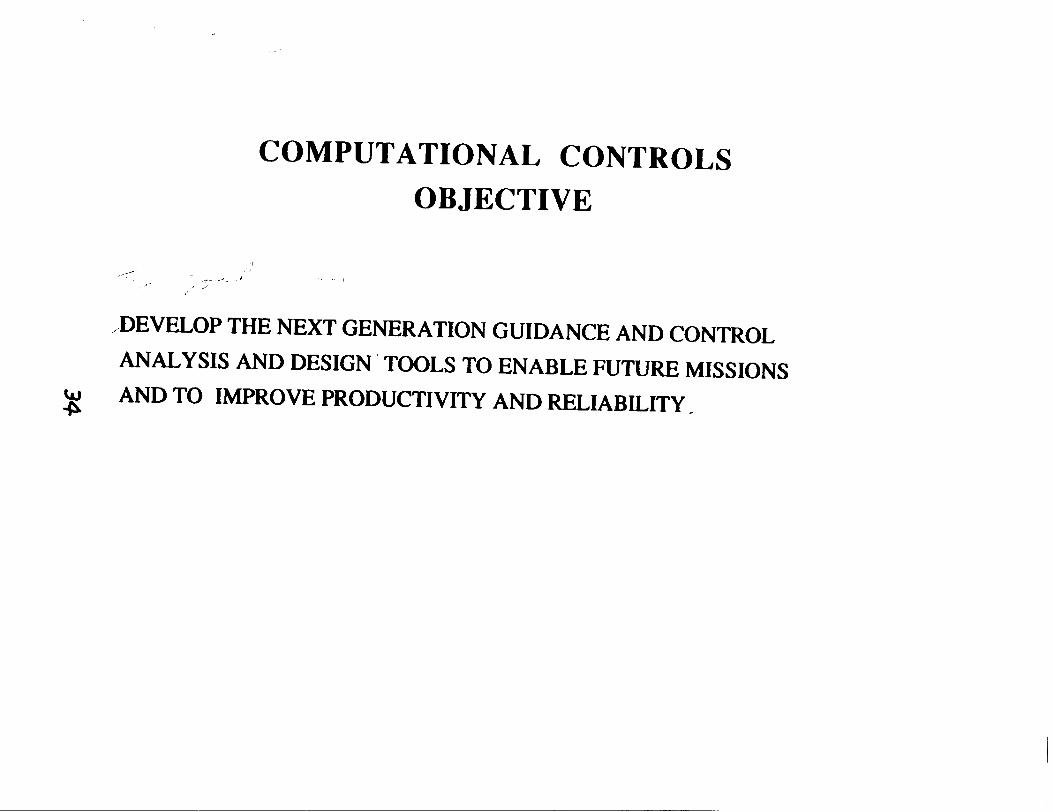


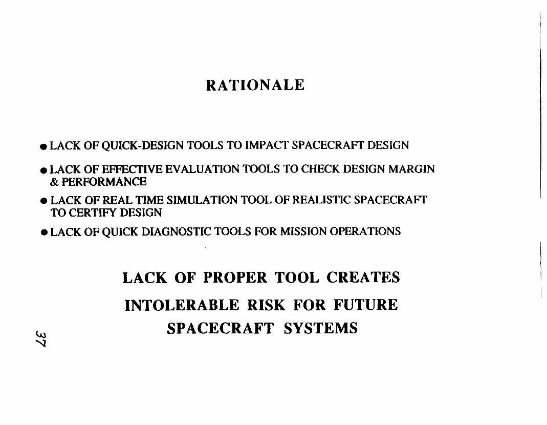
RATIONALE
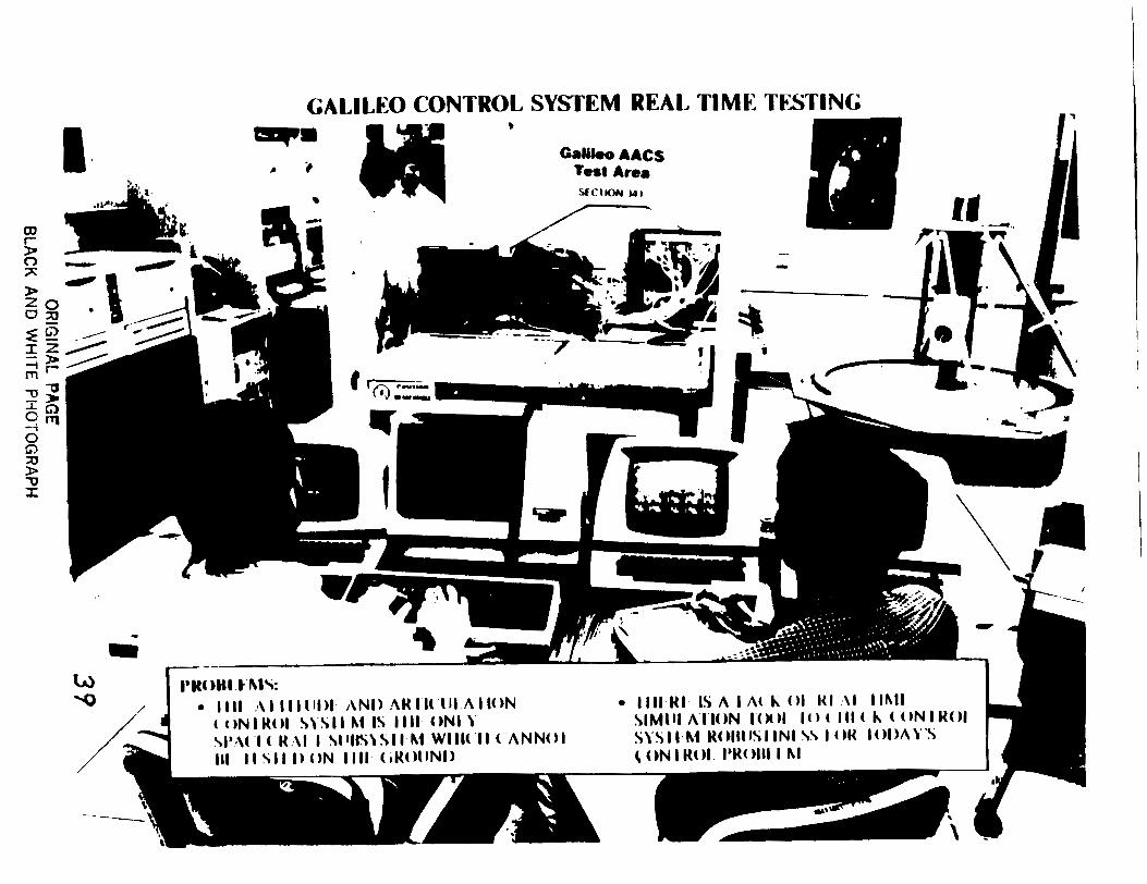
LACK OF QUICK-DESIGN TOOLS TO IMPACT SPACECRAFT DESIGN
LACK OF EFFECTIVE EVALUATION TOOLS TO CHECK DESIGN MARGIN & PERFORMANCE
a LACK OF REAL TIME SIMULATION TOOL OF REALISTIC SPACECRAFT TO CERTIFY DESIGN
LACK OF QUICK DIAGNOSTIC TOOLS FOR MISSION OPERATIONS
LACK OF PROPER TOOL CREATES
INTOLERABLE RISK FOR FUTURE SPACECRAFT SYSTEMS

THE CALILEO CONTROL DESIGN PROBLEM
LACK OFQUICK-LOOK TOOL LEADS TO FAILURE m MEET MISSKIN REQUIREMENTS
IN BEARING ASSEMBLY
SCAN ACIUATOU eon CONraot loos,
LACK OF EFFECllVE EVALUATION TOOL PROHIBITS US FROM IDENTIFYING A MISSION CATAS?ROPHIC FAILURE DURING VENUS ORBIT INSERTION
2
MAGELLAN SPACECRAFT VENUS ORBIT INSERTION PROBLEM
OR
IGIN
AL PAG
E B
LAC
K A
ND
WH
ITE
PH
OTO
GR
AP
H

MISSION OPERATIONS SUPPORT IS INADEQUATE
PROBLEM: LACK OF QUICK DIAGNOSTIC TOOL FOR ANOMALY INVESTIGATION LEAD CONCERNS IN TURN AROUND TIME FOR OPERATIONS

GROWTH IN SPACECRAFT MODELING COMPLEXITY
L O M S T 1- aMMES 8-t STATES H r n )#clsKlN
6ilr ~ E ~ R A T I C M U TOOLS

EVOLUTION OF EARTH OBSERVING PLATFORMS
CHALLENGES: RlINIIffi OF LARGE ARRAY AND AMENNA MULTIPLE BORESIGHT REGlSlRATION ANTENNA SHAPE DEIERMINATION AND ELECTRONIC ALIGNMENT

ADVANCED ASTROPHYSICAL INSTRUMENTS
ASTROPHYSICAL INTERFEROMETER
CHALLENCFS: SHAPE DETERMINATION AND ACTIVE CONTROL SUBWAVELENGTH PHASING OF OmlCAL PATHS DISRIBUTED SENSING AND ACTUATION

MODEL aMPLExm (N-)
CONTROL DESIGN AND ANALYSIS NEEDS VS. CAPABILITIES
EXISTING TOOLS ARE A LIMITING FACTOR IN TODAY'S CONTROL DESIGN AND VERIFICATION, AND ARE INADEQUATE FOR FUTURE NEEDS
--
-
CURRENT CAPABILITIES
NUMBER OF I I I IMPORTANT I I SYSTEM
10 100 1000 STATES

COMPUTATIONAL CONTROLS APPPROACH
ASSESSMENT & RE-NT D E m O N S
NEXT GENERATlON G&C DESIGN & ANALYSIS TOOLS

COMPUTATIONAL CONTROLS APPROACH CONT.
A. TECHNOLOGY ASSESSMENT & REQUIREMENT DEFINITIONS
MULTIBODY SIMULATION TECHNOLOGY VERIFICATION
CONTROL SYSTEM DESIGNIANALYSIS TOOL ASSESSMENT
REQUIREMENT DEFINITION AND ANALYSIS
B. EXISTING TOOLS UPGRADE
UPDATE TOOLS WITH KNOWN DEFICENCIES
UPGRADE TOOLS TO MEET NEAR TERM NEEDS
C. NEXT GENERATION TOOLS DEVELOPMENTS
MULTIBODY SIMULATION TOOLS
CONTROL SYSTEM OPTIMIZATION
TOOLS FOR MODERN COMPUTING ENVIRONMENT
ACCURATE SURFACE MODELING & REPRESENTATION TOOLS
INTEGRATED CONTROL DESIGN ENVIRONMENT

MULTIBODY SIMULATION ASSESSMENT & VERIFICATION PLAN
PLAN SUMMARY:
ESTIMATED DURATION: ON-GOING
START FY 88 FY 89 A ,VERIFICATION
I 1011 187 f Y l O l l l l 8 8 j 1011189
MUST PRELIMINARY COMMITTEE ASSESSMENT MEETING
SCHEDULE:
1ST YEAR
2ND YEAR
REQUIREMENT DEFINITION AND ANALYSIS
ESTABLISH VERIFICATION LIBRARY
TEST CASE DEVELOPMENT
TEST CASE EXECUTION AND EVALUATION
EXPERIMENT EXECUTION AND EVALUATION
TEST REPORT GENERATION
FUTURE YEARS: CONTINUE TO BUILD VERIFICATION LIBRARY
VERIFY NEW TOOLS AS THEY ARE DEVELOPED
DELIVERABLES: QUESTIONNAIRES
REQUIREMENTS MATRIX TEST PLAN TEST CASE REPORT
FINAL REPORT TWO WORKSHOPS
COMPUTATIONAL ASPECTS OF FLEXIBLE BODY SYSTEMS
FINAL REPORT TO THE COMMUNITY


OR1GIIV.AL PAGE lS OF POOR W A L ~
ADDITIONAL SOFTWARE DEVELOPMEN'IS WANTED FOR MODELING AND CONTROL OF FLEXIBLE SPACE SYSTEMS
Dr. Jlguan Gene Lin Control Research Corporation
Lexington, Massachusetts
ABSTRACT
15xisllng modeling and control software packages are elther inadequate or inefficient for i~ppllcatlons to flexible space structures. Some additional software developnlents are wilnlcd for eITecllve design and evalualion of the control systems. The following M 4 - w --. tlfsc~ ~ s s r d , ~ p r e s e T i f a t I o i i :
1 . 1,irlear-quadratlc optimal regulators a s usual can be designed using various "modem rantrol" deslgn software packages. To design for active augmentation of (approximately) lhr S D ~ active -to each "controlled modes." the common practice is lo ;~clJusl repeatedly the state and control welghts (1.e.. the Q and R matrices) by mostly ~~ritllrss trial and error. The tlme consumed and elIbrt spent in the trial-and-error t.c+pcl il Ion can be saved by using an analytical procedure for closely estlmatlng the corn.\l)orlding state and control weights. Varbus ~ m m r l c a l - e x a m p t t s ~ shewn that t l&ia possible. No software has been developed for automat lng such a time-saving ;irl;tlytlcal asslgnment procedure yet.
2. "Modal dashpots" are very effective output-feedback vibrallon controllers for flexlble s l r~~clurcs . not only eflective for augmenting a small amount of actlve damping to a large rluniber of vlbration modes (like the so-called low-authority structural controllers], but also gjJeclive for -~ression of largg vibrallorlg (like high-authority structural controllers]. Recent numerical results on orbital SCOLE configuration have shown SO. NO software has been developed for facilitating the deslgn process yet.
: The aclual performance of any control deslgn needs to be evaluated against a faithful rilodel of the flexlble structure to be controlled. The potentlal of destabfllzation or serlous oerfornlance degradation needs to be detected by numerical simulation of the structure with Lhe control loops being closed. Except for some trivial cases, reduced=order normal- rnode models are generally not appropriate: if they are computationally feasible to slnlulale the closed-loop system. then they are likely not accurate enough to represent the dynan~ics of the flexible structure; U they are satisfactorlly accurate. then they are mostly loo large for eficlive dynamic simulalion even by a state-of-the-art mainframe computer. ikx+k&-eetftpnttnp wry-large m 6 e d ~orrnaf modes Is very expenswe. and f he ;~ccrrrnt~lated computational errors in the natural freq6encies and mode shapes grow very rapidly. The popular Cuyan reductlo chnlque 9 often used to reduce the large flnlte- clcnlrnl mass-slUTness model first. S%,reductlon technique. unlorlunately. introduces large addltlonal errors which are p~oportional to the square of the natut%l frequency of the modes computed thereafter.
'
,,

There Is a trend towards some lnnovatlve use of non-normal modes (such as Rltz or Lancms vectors) for representing the slructures by a much smaller number of such modes. Available resulls are lnterestlng and promising. Mdltional development effort 1s needed and will be very worthwhile.

ADDITIONAL SOFTWARE DEVELOPHENTS WANTED FOR
MODELING AND CONTROL OF FLEXIBLE SPACE SYSTEMS
WORKSHOP ON COMPUTP.TIOF!AL ASPECTS I N THE CONTROL OF FLEXIRLE SYSTEMS JULY 12-14, 1988
WILLIAMS BURG^ VIRGINIA

ADDITIOrIAL SOFTWARE DEVELOPMENTS URGENTLY WPNTEP
@ A ~ ~ I W ~ ~ : P _ R _ ~ S ~ R ~ I N G COMPUTATIONALLY EFFICIENT Lo-OJDINATE PED~JJTION OF FINITE-ELEMENT-MODELS,
To ENARLE
1, PRE-DESIGN OPEN-LOOP DYNAMIC ANALYSIS OF
REALISTIC, LARGE# FLEXIBLE SPACE STRUCTURES AND
@ &_A_~_V_TJ_C~~-SELECT_I_O_N__~F CONTROL AND STATE WE I GHTS)
TO A I D

ACCURACY-PRESERVING COMPUTATIONAL1-Y ECFICI5NT COORDINATE liEDUCTION OF FINITE-ELEVENT flODEI-S
NEEDS
1, CAREFUL PRE-DESIGN OPEN-LOOP DYNAMIC ANALYSI s OF
THE SPACE STRUCTURE^ AND
2, CAREFUL POST-~ESIGN FULL-ORER CLOSED-LOOP EVALUATION OF
CONTROL SYSTEMS FOR THE S T R U C T U ~ E
NEEDS PRE-DESIGN OPEN-LOOP DYNAMIC ANALYSIS -- TO ASSESS EFFECTS OF DISTURBANCES ON SYSTEM PERFORMANCE1
€,Gar POINTING STABIL ITY I 1-INE-OF-SIGHT ERRORS1 I,,
-'- TO IDENTIFY STRUCTURAL MODES NEEDING ACTIVE CONTRO',
-- TO FORM A COMPUTATIONALI-Y FEASIBLE
REDUCED-ORDER CONTROL'D5 SIGN MODEL
-- TO ASSSESS EFFECTIVENESS OF CONTROI- ACTUATORS AND SENSORS
NEEDS POST-DE SI GN FULL-OSDES CLOSED-LOOP EVACUATION -- TO DETECT POSSIBLE INSTABIL ITY INTRODUCED BY
REDUCED-ORDER CONTROL DESIGN
-- TO VERIFY ACTUAL TIME-DOMAIN PERFORMANCE
-- TO TEST ROBUSTNESS TO MODELING ERHORSl PARAMETER VARIATIONS, m a ,

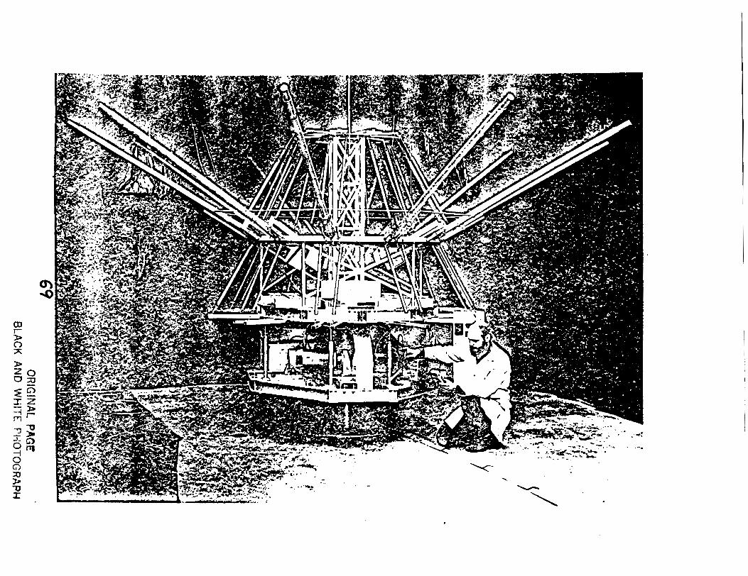
Fig. 1-1 Spacecraft Control Laboratory Experiment (SC0LE)-- the orbital Shuttle-Mast-Antenna configuration.

Fig"" I . A P c , s s i b l t % ELIS P o l a r P l o ~ f c ~ r m ('tlnf igurat i o n
EARTH
SWATH 1- /-
I I
A ILLUMINATION I FOOTPRINT
F ,gun. 2 . SAR 1 r n . t ~ l n e l:? < IILL t r y
ORIGINAL PAGE ;S OF POOR QUALITY
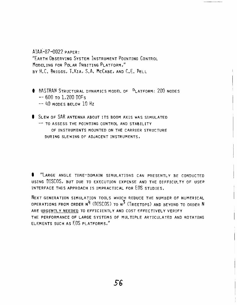
0 SLEW OF SAR ANTENNA ABOUT ITS BOOM AXIS W A S SIMULATED
-- TO ASSESS THE POINTING CONTROL AND STABIL ITY
OF INSTRUMENTS MOUNTED ON THE CARRIER STRUCTURE
DURING SLEWING OF ADJACENT INSTRUMENTS
@ "LARGE ANGLE TIME-DOMAIN SIMULATIONS C A N PRESENTLY RE CONDUCTED
USING nIscos, BUT DuE T o EXECUTION EXPENSE AND THE DIFFICUCTY OF USER
INTERFACE THIS APPROACH IS IMPRACTICAL FOR EOS STUDIES,
NEXT GENERATION SIMULATION TOOLS WHICH REDUCE THE NUMBER OF NUMERICAL
OPERATIONS FROM ORDER N4 (I)ISCOS) TO N3 (TREETOPS) AND BEYOND TO ORDER N ARE U_RJ_E_NTLY NEEDED TO EFFICIENTLY AND COST EFFECTIVELY VERIFY
THE PERFORMANCE OF LARGE SYSTEMS OF MULTIPLE ARTICULATED AND ROTATING
ELEMENTS SUCH AS EOS PLATFORMS, I 1
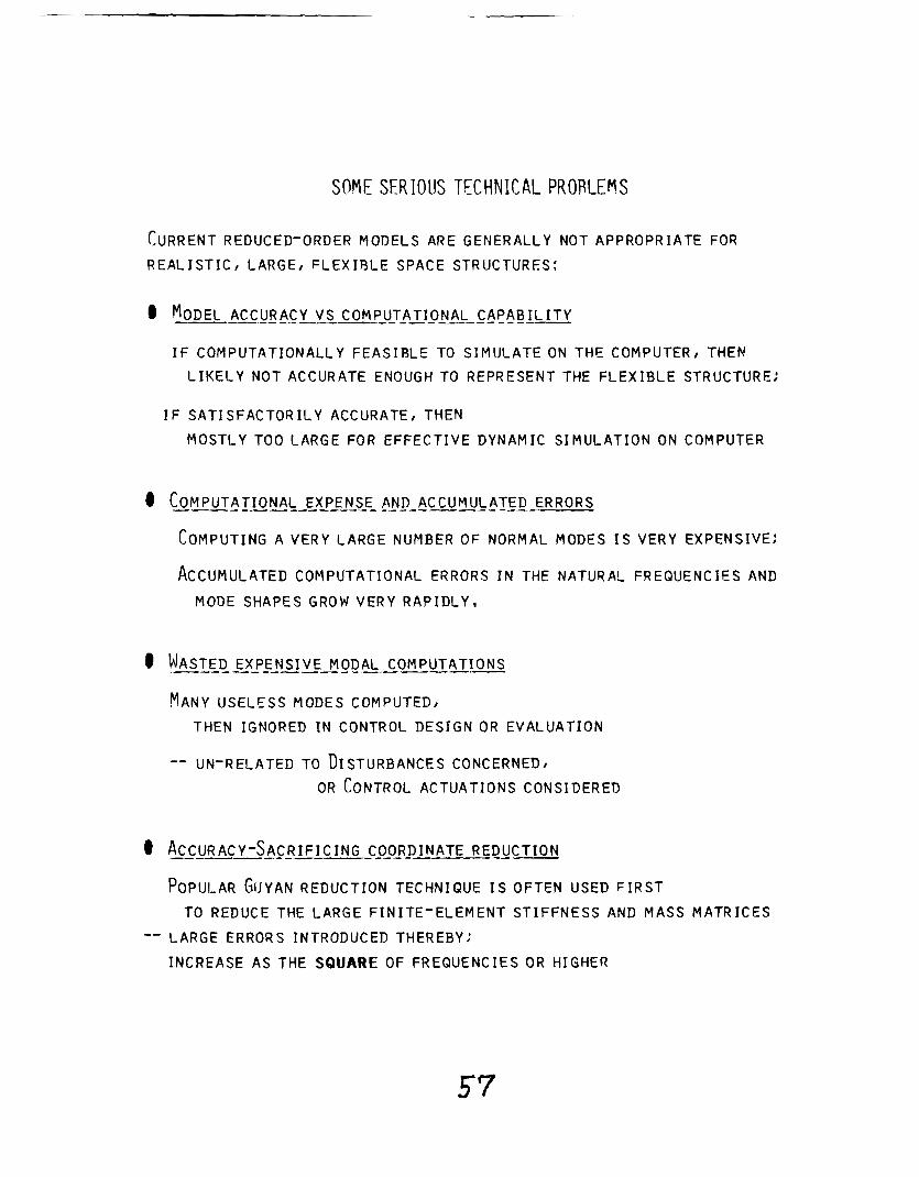
SOME SERIOllS TECHNICAL PR0RLEM.S
CURRENT REDUCED-ORDER MODELS ARE GENERALLY NOT APPROPRIATE FOR
REALISTIC , LARGE, FLEXIBLE SPACE STRUCTURES:
I F COMPUTATIONALLY FEASIBLE TO SIMULATE ON THE COMPUTER, THEN
L I K E L Y NOT ACCURATE ENOUGH TO REPRESENT THE FLEXIBLE STRUCTURE;
I F SAT1 SFACTORILY ACCURATE, THEN
MOSTLY TOO LARGE FOR EFFECTIVE DYNAMIC SIMULATION ON COMPUTER
ACCUMULATED COMPUTATIONAL ERRORS IN THE NATURAL FREQUENCIES AND
MODE SHAPES GROW VERY RAPIDLY n
MANY USELESS MODES COMPUTED,
THEN IGNORED I N CONTROL DESIGN OR EVALUATION
-- UN'RELATED TO DISTURBANCES CONCERNED,
OR CONTROL ACTUATIONS CONSIDERED
POPIJLAR GIJYAN REDUCTION TECHNIQUE IS OFTEN USED FIRST
TO REDUCE THE LARGE FINITE-ELEMENT STIFFNESS AND MASS MATRICES
-- LARGE ERRORS INTRODUCED THEREBY:
INCREASE AS THE SQUARE OF FREQUENCIES OR HIGHER

INNOVATIVE: RAYLEIGH-R ITZ METHOD
A TREND TOWARDS SOME INNOVATIVE USE OF NON'MORMAL MODES
(SIJCH A S RITZ O R LANCZOS VECTORS) FOR REPRESENTING THE STRUCTURES B Y
A MUCH SMALLER NUMBER OF GENERALIZED COORDINATES
-- AVAILABLE RESULTS INTERESTING AND PROMISING,
-- ADDITIONAL DEVELOPMENT AND EXTENTION EFFORTS NEEDED,
-- ORIGINAL L A R G E MATRICES M AND Y\ NOW REDUCED TO
SMALLER ONES:
M = 0 T r l 0 , C
KC = CIT K O
0 W I L S O N - Y _ ~ _ ~ _ N ~ ~ J C K E N S _ A _ ~ G ~ O R I T H M
-- ASSUME F(T) = B u(T), U(T) = A SCALAR FUNCTION

ADDITIONAL DEVELOPMEPIT AND EXTENTION EFFORTS WANTED
2, COMPUTATIONAL INTENSIVE: PERFORM GRAM-SCHMIDT ORTHOGONALIZATION
E V E R Y T I M E A VECTOR Q * I S G E A N E R A T E D I
-- NOUR-OM ID AND CLOUGH' s SOLUTION W A S TO ORTHOGONAL IZE
O N L Y W I T H R E S P E C T TO TWO P R E V I O U S V E C T O R S ,
-- THE MOST TROUBLESOME DRAWBACK OF THE LANCZOS ALGORITHM
R E A P P E A R :
EASY LOSS OF ORTHOGONALITY OF THE LANCZOS VECTORS;
RE 'ORTHOGONAL IZAT ION R E Q U I R E D WHEN O R T H O G O N A L I T Y I S L O S T
-- THE WILSON-YUAN-~ICKENS ALGORITHM WAS FORMULATED FOR
SCALAR FORCES:
N O T D I R E C T L Y A P P L I C A B L E TO T H E G E N E R A L CASE O F
MULTIPLE SIMULTANEOUS DISTURBANCE (OR CONTROL) FORCES
-- RUT, SPACE SYSTEMS LIKELY BE SUBJECT TO MULTIPLE DISTURBANCES
N O T O N E A T A T I M E , B U T S I M U L T A N E O U S L Y

LINEAR-QUADRATIC REGULATORS (LflR) FOR FLEXIBLE SPACE STRUCTURES
W I T H
r ~ l f I I 1 ° 2 1
n = 1 I I ' I I 0 I
I S M I N I M I Z E D W I T H U = [ X
0 GIVEN THE CONTROL AND STATE WEIGHTING MATRICES R AND (3,
ANY "MODERN CONTROL" DESIGN PROGRAM, SUCH ORACLS, CTRL-C, C A N P R O D U C E AN O P T I M A L S O L U T I O N K V I R T U A L L Y A U T O M A T I C A L L Y

DESIGN OF LINEAR-QUDRATIC REGULATORS FOR A C T I V E AUGMENTATION OF SPECIFIIED OAMPING TO SPECIFIC MODES
A_PPRAOACH 1, CONSTRAINED OPTIMIZATION
OPTIMIZE THE PERFORMANCE INDEX J WITH THE SPECIFIED DAMPING RATIOS
AS CONSTRAINTS,
-- CONSTRAINED OPTIMIZATION IS PARTICULARLY COMPLICATED
WHEN DYNAMIC EQUATIONS ARE INVOLVED
-- SOME MODES M A Y NOT GET ENOUGH DAMPING TO BE CLOSE TO THE SPECIFIED,
WHILE SOME OTHERS MAY GET TOO MUCH MORE THAN THE SPECIFIED,
START WITH DIAGONAL R AND Q WITH SOME ARBITRARY NUMBERS, E , G , , 1: CARRY OUT THE DESIGN O F THE CORRESPONDING LOR; EVALUATE THE CLOSD'LOOP POLES, AND HENCE THE DAMPING RATIOS,
TRY OTHER CONTROL AND STATE WEIGHTS,
REPEAT THE DESIGN-EVALUATION CYCLE,
UNTILL THE RESULTS ARE SATISFACTORY n
-- THE CONTROL AND STATE WEIGHTS USED MOSTLY ARE AD HOC:
THE TRIAL'AND'ERROR PROCESS I S MOSTLY ENDLESS,
VERY TIME CONSUMING

ADDITIONAL SOFTWARE DEVELOPMENT WANTED
SOFTWARE MODULES FOR AIDING DESIGNERS IN MAKING GOOD IWITIAL CHOICES,
AND INTERMEDIATE ADJUSTMENTS, OF THE CONTROL AND STATE WEIGHTS
SO THAT ,
THE RESULTING DESIGN OF LINEAR-QUADRATIC REGULATORS
CAN/ W_LTTHIN ONLY A FEW ITERATIONS/ SATISFY CLOSELY
THE DESIGN SPEC1 FICATIONS I
E ,G , r ON DAMPING AUGMENTATION4 STIFFNESS AUGMENTATION/
CINE-OF-SIGHT POINTING ACCURACY r ETC,

ADDITIONAL SOFTbIARE DEVELOPMENTS URGENTLY WANTEn
@ ACCURACY-PRESERVING _ _ . _ _ - _ _ _ _ _ _ _ _ _ _ - _ . _ COMPUTATIONALLY EFFICIENT __- COORDINATE -- - - -- - - REDUCTION - - . OF FINITE-EL-E_M_EN~-MODELS,
To ENABLE
1, PRE-DESIGN OPEN-LOOP DYNAMIC ANALYSIS OF
REALISTIC, LARGE, FLEXIBLE SPACE STRUCTURES AND
0 ~ A L Y T I C A L SELECTION OF C ~ ~ ~ Q ~ - ~ ~ N _ ~ _ > ~ _ T _ E - W E I G H T S ,
TO A ID
~ E S I G N OF LINEAR-QUADRATIC REGULATORS DESIRED FOR
VIBRATION CONTROL OF FLEXIBLE SPACE STRUCTURES

SESSION I1 - SURVEY OF AVAILABLE SOFTWARE
PRECEOING PaGE BLANK NOT FILMED

FtJFlXIBLE STRUCTURE CONTROL EXPERIMENT8 USING A REAL-TIME WORKSTATION FOR C O m R - A I D E D CONTROL ENGINEERING
Michael E. Stleber Communications Research Centre
Ottawa, Ontario. CANADA
ABSTRACT
A Iieal-Time Workstation for Computer-Aided Control Englneerlng has been developed jolnt ly by the Conmunlcatlons Research Centre (CRC) and Ruhr-Unhrersitaet Bochum (RUD). West Germany. The system is presently used for the development and experimental verillcation of control techniques for large space systems with slgnlficant struclural flexibility.
- 1 7 1 ~ Real-Time Workslation 4dAtttdrmerti-U essentially is an implementation of l i U n ' s extensive Computer-Aided Control Englneerlng package "KEDDC on an I N E L ~nlcro-computer runnlng under the RMS real-time operating system. The portable system supports system identification. analysls, control design and simulation, as well ;IS the ilnmedlale Implementation and test of control systems. Auealth dclasskal ;indndem eontrot analysfs-anci design methods are available to the user who latt-Cthmugh a frler~dly dfaiog; The we~k4tattm carrbe configured bolh,.wilh anetog and digitat interfaces to the "real work!" fofdata acquisition and c~nC rol.
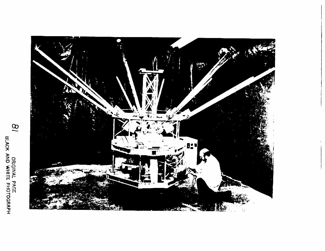
'I'he Real-Tlme Workstation is currently being used by CRC to study control/structure lrileractlon on a ground-based structure called "DAISY' (cf, Atta~hment 2). whose design was Inspired by a reflector antenna. DAISY emulates the dynarnlcs of a large flexible spacecraft wlth the following characteristics: rigld body modes. many clustered vibration modes wilh low frequencles and extremely,_low damping. DAISY presently lias seven control actuators and eight sensors which are all "spacecralt-like."
'The class of control algorithms currently investigated by experiments is "robust LQG" ron(ro1. The Real-Tlme Workstallon was found to be a very powerful tool for experimental studles. supporting control design and slmulation. and conducting and evalualing lesls wilhln one integrated environment. -y trrrea3cd +he flexlbilrty and.tutnarotlnd of ZAe experiments. As the Workstation all but eliminates the barriers between ideas on control systems and their experimental evaluation. analyllcal and experlmental development can take place essentially simultaneously.
PRECEDlNG PAGE BLANK NOT FILMED

REAL-TIME WORKSTATION FOR
COMPUTER-AIDED CONTROL ENGINEERING
6Y
O
RIG
INA
L PAG
E B
LAC
K A
ND
WH
ITE
@H
OTO
GR
AP
H

FLEXIBLE STRUCTURE CONTROL EXPERIMENTS
USING A REAL-TIME WORKSTATION FOR
COMPUTER-AIDED CONTROL ENGINEERING
MICHAEL E. STIEBER
SPACE MECHANICS DIRECTORATE
COMMUNICATIONS RESEARCH CENTRE, OlTAWA, CANADA
SPONSORED BY: SPACE-BASED RADAR PROGRAM DEPARTMENT OF NATIONAL DEFENCE, CANADA
NASA WORKSHOP ON COMPUTATIONAL ASPECTS IN THE CONTROL OF FLEXIBLE STRUCTURES, JULY 12-1 4,1988
OUTLINE
1. INTRODUCTION
2. REAL-TIME WORKSTATION - CAPABILITIES
- HOST ENVIRONMENT
-4 - 3. FLEXIBLE STRUCTURE CONTROL EXPERIMENT
- CHARACTERISTICS
- APPLICATION OF REAL-TIME WORKSTATION
4. SUMMARY & CONCLUSIONS

SPACE-BASED RADAR
SPACE-FED PHASED ARRAY ANTENNA CONCEPT

TECHNOLOGY DEVELOPMENT FOR
CONTROL OF FLEXIBLE SPACE STRUCTURES
- ANALYTICAL STUDIES DEVELOPMENT OF NEW TECHNIQES APPLICATION TO STRAWMAN PROBLEMS (SIMULATIONS)
- GROUND-BASED EXPERIMENTS VALIDATION AND DEMONSTRATION OF ANALYTICAL RESULTS
SUPPORT BY CAD SYSTEMS ?

HOW DO CAD PACKAGES SUPPORT
CONTROL SYSTEM TECHNOLOGY DEVELOPMENT ?
MANY SUPPORT ANALYTICAL STUDIES - NUMERICAL ANALYSIS
- GRAPHICS
FEW DIRECTLY SUPPORT EXPERIMENTAL STUDIES, WHICH REQUIRES: - INTERFACE TO THE REAL WORLD
- DATA ACQUISITION
- IMPLEMENTATION & TEST OF REAL-TIME CONTROL SYSTEMS

REAL-TIME WORKSTATION FLEXIBLE STRUCTURE CONTROL EXPERIMENT
- SYSTEM I SIGNAL ANALYSIS - CONTROL DESIGN
- SYSTEM IDENTIFICATION - RT CONTROL OPERATION

REAL-TIME WORKSTATION SOFTWARE
UNDERLYING CAD PACKAGE: KEDDC
- DEVELOPED BY DR. CHRISTIAN SCHMID
- AT RUHR-UNIVERSITY, BOCHUM, WEST GERMANY
- RT WORKSTATION A JOINT PROJECT OF RUHR-U. AND CRC
FEATURES - MATURE
- COMPREHENSIVE
- PORTABLE (RUNNING UNDER 12 OPERATING SYSTEMS)
- MODULAR, OPEN SYSTEM

CORE MODULES
- MATRIX MANAGER
- SYSTEM MANAGER
- FREQUENCY MANAGER
- SIGNAL MANAGER
- POLYNOMIAL MATRIX MANAGER
- GRAPHICS MANAGER
CAPABILITY OF CORE PACKAGE - INTERACTIVE 'CALCULATOR* -TYPE ENVIRONMENT
- 250 COMMANDS
- EXTENDED BY APPLICATIONS MODULES

HOST ENVIRONMENT
REQUIREMENTS FOR SELECTION
REAL-TIME MULTI-TASKING OPERATING SYSTEM
- PORTABLE COMPUTER
- COMPATIBLE WITH FUTURE MICRO-PROCESSORS
SYSTEM CHOSEN (IN 1985): INTEL 286/310
- OPEN SYSTEM (MULTIBUS 1)
- CPU: INTEL 80286180287
- OPERATING SYSTEM: INTEL RMX86
- UPGRADE TO 386-BASED RMX286 SYSTEM PLANNED

HOST ENVIRONMENT (CONT'D)
PERIPHERALS
- GRAPHICS TERMINAL (780 X 1024 RESOLUTION)
- DOT MATRIX PRINTER
REAL-TIME SIGNAL INTERFACE FOR DATA ACQ. AND CONTROL
- IEEE 488 GPlB (USED IN FLEXIBLE STRUCTURE CONTROL EXPERIMENT)
- ANALOG SIGNALS
DATA LINK TO REMOTE MAINFRAME

REAL-TIME WORKSTATION FLEXIBLE STRUCTURE CONTROL EXPERIMENT
- SYSTEM / SIGNAL ANALYSIS
- SYSTEM IDENTIFICATION
------ - -----
ORIG
INAL PAG
E B
LAC
K A
ND
WH
ITE PH
OTO
GR
AP
H

DAISY: A FLEXIBLE SPACECRAFT EMULATOR
r Wol I I

DAISY
EMULATES DYNAMICS OF A LARGE FLEXIBLE SPACE STRUCTURE
- 3 RIGID-BODY MODES (SLIGHT PENDULOSIN IN 2 RIGID-BODY MODES)
- 20 FLEXIBLE BODY MODES, LOW FREQUENCIES: 0.07 ... 0.11 Hz, IN CLUSTERS
- LOW DAMPING RATIO ACHIEVED
RIBS: 0.008, HUB: 0.01 ... 0.05
SPACECRAFT - LIKE SENSORS AND ACTUATORS
- 3 REACTION WHEELS ON HUB
- THRUSTERS ON RIB(S)
- ENCODERS ON HUB GIMBAL
- ACCELEROMETERS ON RIB(S)
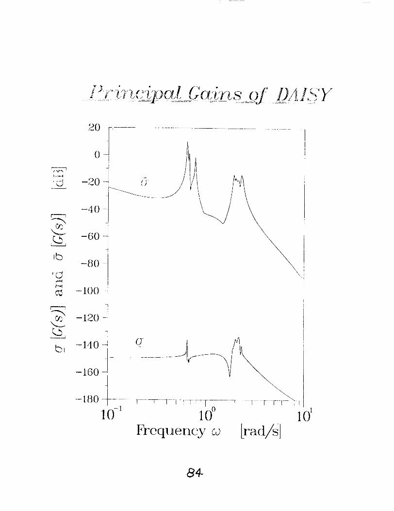
Frequency w [rad/s]
84

EXPERIMENTAL RESEARCH USING DAISY
PRESENT OBJECTIVE
DEVELOPMENT AND DEMONSTRATION OF
ROBUST CONTROL ALGORITHMS FOR FLEXIBLE STRUCTURES
STEPS (NOT NECESSARILY IN THIS ORDER)
- GIVEN: ANALYTICAL DYNAMICS MODEL
- SYSTEM-ORDER REDUCTION
- MODEL DISCRETIZATION
- SYNTHESIS OF CONTROL ALGORITHM
- SIMULATION
- EXPERIMENT
- EVALUATION OF ALGORITHM
TURNAROUND: 40 MIN

DESIGN EXAMPLE
SYSTEM EIGENVALUES AND TRANSMISSION ZEROS MODEL (SYSTEM MATRIX)

REAL-TIME CONTROL OPERATION
INTERACTIVE MONITOR
- INTERFACE BETWEEN USER AND REAL-TIME CONTROL ALGORITHM
- CONFIGURATION AND CONTROL OF REAL-TIME ALGORITHM
- DISPLAY AND RECORDING OF EXPERIMENTAL RESULTS SIGNALS: PLANT INPUTIOUTPUT, SETPOINTS, OBSERVER STATES, ...
- COMPLETE ENVIRONMENT FOR EFFICIENT EXPERIMENTATION
REAL-TIME CONTROL ALGORITHM
- EXECUTION TIME
EXTREMES: 5 MlLLlSEC WlTH 5TH-ORDER OBSERVER 1.2 SEC WlTH SOT"-ORDER OBSERVER, 10 INPUTS, 10 OUTPUTS
TYPICAL FOR DAISY APPLICATION (2OTH-ORDER, 5 INP, 5 OUTP): 20 MlLLlSEC
- HOST FAST ENOUGH FOR REAL-TIME CONTROL OF DAISY SAMPLING INTERVAL: 0.2 SEC ... 1 SEC

SUMMARY
EXPERIMENTAL RESEARCH ON CONTROL OF FLEXIBLE STRUCTURES
"DAISY"
CONCLUSION
REAL-TIME WORKSTATION BRIDGES GAP BETWEEN THEORY AND EXPERIMENT!

CONSOLE: A CAD TANDEM FOR OPTIMIZATION-BASED DESIGN INTERACTING WITH USER-SUPPLIED SIMWATORS
Michael K. H. Fan. L1-Sheng Wang. Jan Konincloc and Andre L. Tits University of Maryland College Park. Maryland
ABSTRACT
The most challenging task when designing a complex engineering system is that of coming up wlth an appropriate system "structure." This task calls extensively upon the engineer's ingenuity. creatlvlty. lntultion and experience. Alter a structure has been (maybe temporarily) selected. it remains to determine the "best" value of a number of "deslgn parameters." The engineer's input is still essential here, a s multiple tradeofls are bound to appear. However, except in the simplest cases. achieving anything close to optimal would be lmposslble without the support of numerical optimization. Providing such support while emphasizing tradeoff exploration through man-machine Interaction is the purpose of interactive optimization-based design packages such a s CONSOLE (Proceedings of American Control Conference 1988). A requlrement for CONSOLE 1s that the parameters to be optimally adjusted vary over a continuous (as opposed to discrete) set of values.
CONSOLE employs a recently developed design methodology (Internatlonal Journal of Control 43: 1693- 172 1) which provides the designer with a congenial envlronment to express his problem as a multiple objective constrained optimization problem and allows him to reflne his characterkation of optlmality when a suboptimal design is approached. To this end. in CONSOLE. the designer formulates the deslgn problem using a high-level language and performs design task and explores tradeon through a few short and clearly defined commands.
The range of problems that can be solved efficiently using a CAD tools depends very much on the abllity of this tool to be interfaced wlth user-supplied simulators. For instance, when designing a control system one makes use of the characteristics of the plant, and therefore. a model of the plant under study has to be made available to the CAD tool. CONSOLE allows for an easy interfacing of almost any simulator the user has available.
To dale CONSOLE has already been used successfully In many applications, including the design of controllers for a flexible arm and for a robotic manipulator and the / solullon of a parameter selectlon problem for a neural network (all under P. S. i Krfshnaprasad at the University of Maryland at College Park), the design of an RC I I
controller for a radar antenna (under F. Emad at the University of Maryland at College I Park). and the design of power filters (at the Westinghouse Defense and Electronics Center). In the case of the neural network application. CONSOLE was coupled to the ,' nonlinear system simulator SIMNON.

CONSOLE :
A CAD Tandem for Optimization-Based Design Interacting with User-Supplied
Simulators
Michael K.H. Fan Li-Sheng Wang Jan Koninckx Andrk L. Tits
Systems Research Center University of Maryland, College Park

HISTORY
DELIGHT (Nye, Polak, Sangiovanni-Vincentelli, Tits) 1980
general purpose interactive package + optimization algorithms
DELIGHT.MaryLin (Fan, Nye, Tits) 1985 - interactive optimization-based design package for linear time-invariant systems
CONSOLE (Fan, Wang, Koninckx, Tits) 1987 - interactive optimization-based design package for engineering systems (with user-supplied simulators)

CONSOLE
PARAMETRIC OPTIMIZATION IN DESIGN
Assume structure already chosen
Examples :
Circuit --, Topology
Control System -' Controller Structure
Earthquake Proof Building -+ Number and Position of Beams
Remain to choose best value of finitely many parameters
Examples :
Circuit --, R, C, W, A, ... Control System - Controller Gains,
LQRILQG Weighting Matrices, Q-parameterization, ...
Earthquake Proof Building --, Beam Thickness, Amount of Steel, ...
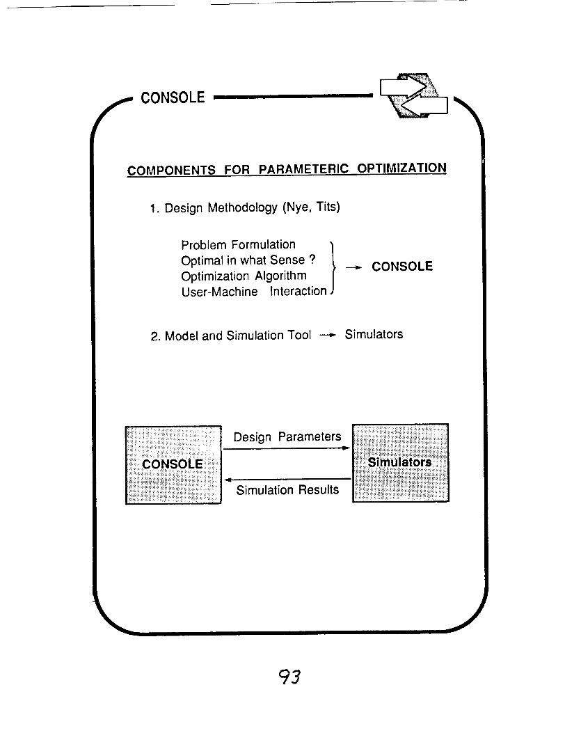
CONSOLE
COMPONENTS FOR PARAMETERIC OPTIMIZATION
1. Design Methodology (Nye, Tits)
Problem Formulation Optimal in what Sense ? I CONSOLE Optimization Algorithm User-Machine Interaction
2. Model and Simulation Tool --, Simulators
Design Parameters e
a
Simulation Results

PROBLEM FORMULATION
I Types of Specifications
- . .
Objectives - The smaller (larger) the better.
Soft Constraints - Aim for a target value. If unachievable,
the smaller (larger) the better.
I Constraints - Specified value must be achieved.

min max f'.(x) I
x i

OPTIMIZATION ALGORITHM
Three Phase Feasible Direction Algorithm
Phase 1 (until all hard constraints are satisfied)
attempt to satisfy hard constraints (HC)
minimax on HC
Phase 2 (until all good values are achieved)
improve objectives (0) and soft constraints (SC)
minimax on 0 and SC
subject to satisfying HC
Phase 3
improve objectives
minimax on 0
subject to satisfying HC and SC

min max f.(x) I
subject to
CONSOLE
-
where
fi(x) = max cp,(x,o) 03

USER-MACHINE INTERACTION
CONSOLE
Purpose
Progressively refine problem definition
Means
Information on status of design conveyed graphically
to user (Pcomb, Ecomb).
User steers design to his optimal solution by adjusting
goodhad values/curves.
98

CONSOLE =
CONvert + SOLVE

CONSOLE
i
OPTIMAL SOLUTION

A SIMPLE DESIGN EXAMPLE
DESIGN SPECIFICATION

f CONSOLE
SYSTEM DESCRIPTION FILE FOR THE EXAMPLE /SiMNON*)
CONTINUOUS SYSTEM servo STATE x l x2 x3 DER dxl dx2 dx3 XI :o x2:O x3:O dxl = x2 dx2 = if (e > 0.4) then 0.4
else if (e < -0.4) then -0.4 else e
dx3 = r - y e = (r - y)'Kp + x3'Ki y = x1+x2 r:1
NON was developed at the Lund Institute of Technology, Lund, Sweden I

CONSOLE
PROBLEM DESCRIPTION FILE FOR THE EXAMPLE
designgarameter Kp init=l variation-5 designgarameter Ki
functional-objective "overshoot" for t from 0 to 20 by 0.1 minimize {
double simnon-time-response(); return simnon~time~response(Kp,Ki,"y".t); 1
good-cu we={ if (t <= 4) return 1.05; else return 1 .01; 1
bad-curve ={ if (t <= 4) return 1.1 ; else return 1.02; 1
functional-objective "settling timew for t from 2 to 20 by .1 maximize {
...
103

CONSOLE
MAIN FEATURES OF CONSOLE
Problem formulation is closely related to the character of a design problem.
Problem formulation syntax is strict, but easy to use.
Efficient iteration between CONVERT and user for debugging the PDF.
SOLVE is interactive, with short and clearly defined commands providing efficient communication between the program and the user.
Interactive graphics provide the user with easy-to-interpret information on the current design (Pcomb, Ecomb).
User-supplied simulators can easily be linked with SOLVE.

r GLANCE AT APPLICATIONS
Design of a copolymerization reactor controller (Butala, Choi, Fan)
Design of controllers for a flexible arm (Wang, Krishnaprasad)
Design of a controller for a robotic manipulator (Chen, Krishnaprasad)
H-infinity Design of Sampled-Data Control System5 (Yang, Levine)
Solution of a parameter selection problem for a neural network (Pati, Krishnaprasad et a/.)
Design of an RC controller for a radar antenna (Emad)
Design of power filters (Glover, Walrath at Westinghouse Defense and Electronics Center)
... and soon
Design of earthquake proof buildings (Austin)
Design of controllers for X29 aircraft (Reilly, Levine)
Design of circuits
L (Westinghouse)

CONSOLE
DESIGN OF A COPOLYMERIZATION REACTOR CONTROLLER
(CONSOLE + Copoly) (Butala, Choi, Fan)
Objectives and Constraints
Molecular Weight Composition Final Volume Temperature Feed Flowrate
Manipulated Variables
Temperature = a, + a,t + a,t2 + a,P Feed Flowrate = b, + bJ + bat2 + b,P
Design Parameters = ai's and b,'s
Results
Pcoab (Itor- 22) (Phare 2) (MAX-COST-SOFT- 0.0766327)
SPECIF1CATIOM FOl (W-UFa)-2 FO2 (CC-CCm) -2
Cl f i n d vol PC1 uppor t r p ?a 10.0~ tmp FC3 uppr 910. PC4 lowor f l a
BAD 2.60e+OT 6 .Oh-02 4.10.+00 s.640*02 3.250+02 7.500-02
-9 .000-05

DESIGN OF A DC DIRECT DRIVE MOTOR
(CONSOLE + Simnon) (Wang, Krishnaprasad)
Objective Position Profile
Design Parameters Feedback Gains
Results

FUTURE ENHANCEMENTS
User Interface
More Powerful Optimization Algorithms
Gradient Computation

THE APPLICATION OF TSIM SOFTWARE TO ACX DESIGN AND ANALYSIS ON FImuBLE AIRCRAFT
Ian W. Kaynes Royal Aerospace Establishment Farnborough. Unlted KLngdom
ABSTRACT
The TSIM software I s described. This is a package whlch uses a n interactive FOHIRAN- like simulatlon language for the simulation on nonlinear dynamic systems and offers facllltles whlch Include: mixed contlnuous and dlscrete time systems, time response calculatlons. numerical optlmlzation. automatic trimming of nonlinear aircraft systems, and linearkation of nonlinear equations for efgenvalues, frequency responses and power spectral response evaluation.
Details are glven of the application of TSIM to the analysis of aeroelastlc systems under the RAE Farborough extension FLEX-SIM. The aerodynamic and structural data for the erluatlons of motion of a flexible aircralt are prepared by a preprocessor program for Ir~corporatlon in TSIM simulatlons. Within the slmulatlon the flexible aircraft model may then be selected Interactively for diflerent flight conditfons and modal reduction tcchnlques applled. The use of FLEX-SIM is demonstrated by an example of the flutter predlction for a simple aeroelastlc model.
By utilklng the numerical optimbatfon faclUty of TSIM It is possible to undertake ldent l~lcatlon of requlred parameters in the TSIM model within the slrnulatlo_n. The optimker is applied to the minlmimtion of error between predicted and measured time responses of the system: whlle possibly not so efficient a s dedicated identincation software this has the great advantages that the ldentiflcation is made directly lrivolvlng the slmulatlon model wlthout furlher reprogramming or data transfer and it may be applled dlrectly to nonllnear models. Examples are glven of this analysis appllcd to alrcrafl measured responses and to simulated responses of a controlled aircraft wlth nonllnearltles.

THE APPLICATION OF TSIM SOFTWARE TO ACT DESIGN AND ANALYSIS ON FLEXIBLE AIRCRAFT
by
IAN KAYNES
ROYAL AEROSPACE ESTABLISHMENT F a r n b o r o u g h , Eng land
Head, T h e o r e t i c a l Dynamics S e c t ion, S t r u c t u r a l Dynamics D i v i s i on ,
M a t e r i a l s and S t r u c t u r e s D e p a r t m e n t
PROGRAMME OBJECTIVES
1 . Improvement o f a e r o e l a s t i c modell ing techn iques
2 . ACT Design methods f o r s t r u c t u r a l app l i ca t ions
3 . Assessment o f s t r u c t u r a l impact o f A C T
2. RAE FLEX-SIM

RAE EXPERIMENTAL PROGRAMMES
3. RAE FLEX-SIM
1 . Flight d a t a f rom f l ex ib le a i r c r a f t (VCIO. Tornado)
2 . Wind tunne l experiments (GARTEUR, ' f l y i n g model', spo i l e r t e s t s )
AEROEL ASTlC MOOELL ING INPUT
a ) STRUCTURAL MODAL DATA Calculated from mass and s t i f f n e s s d a t a by f i n i t e element o r beam models AND/OR der ived from ground resonance t e s t s . Model r e d u c t i o n techniques used as appropr ia te .
b AERODYNAMIC LOADINGS Calculated f rom geometr ic d a t a by v o r t e x l a t t i c e o r RAE methods f o r s teady and unsteady flow.
c 1 SENSOR and ACTUATOR DATA. Linear it y assumed in these models,
1 4- RAE FLEX-SIM I

AEROSERVOELASTIC MODEL
Combinat ion o f s t r u c t u r a l , aerodynamic, senso r and a c t u a t o r d a t a wi th t h e c o n t r o l system model.
Exp ressed in a f i r s t o r d e r f o r m compat ib le with s t a b i l i t y and c o n t r o l r e p r e s e n t a t i o n s t o allow i n t e g r a t i o n between t h e ae roe las t i c i an and t h e S&C s p e c i a l i s t s .
S o f t ware r e q u i r e d f o r r esponse p r e d i c t i o n and c o n t r o l des ign a c t i v i t i e s on t h e s e models.
5. RAE FLEX-SIM
TS I M
Time S IMu la t i on
Non- l inear dynamic s imulat ion package
Or i g i na ted and developed a t RAE s ince l a t e 1970s
Now documented, s u p p o r t e d and developed as a commercial p r o d u c t b y Cambridge C o n t r o l
Used in R A E and in r e s e a r c h o rgan i sa t i ons , ae rospace i n d u s t r y and u n i v e r s i t i e s i n B r i t a i n and o v e r s e a s
6. RAE FLEX-SIM

TSIM FACICITJES
I n t e r a c t i v e p rogram us ing FORTRAN-like s imulat ion language a n d f a c i l i t a t i n g mod i f i ca t i on o f model
Simulat ion o f l i nea r and non - l i nea r equa t i ons Mixed con t inuous and d i s c r e t e time systems Time response c a l c u l a t i o n L i nea r i s a t ion o f non- l inear equa t i ons f o r :
Eigen va lues Frequency responses RMS response eva lua t ion
Numer ica l o p t i m i s a t i o n Automat ic tr imming o f non- l inear a i r c r a f t Communication wi th o t h e r c o n t r o l design packages
7. RAE FLEX-SIM
SAMPLE OF TSIM SERIAL INTERACTION
S I M > S I H > ; Assign values to some T S I M var iab les : - S I M z ZPOSA 0 .9 DAMPA 0 .7 RTB 15 S I N > SIN>; Enter the time response set-up nodule and S I M 2 : def ine the required parameters:- S I N > SET TIME-RESP S I H> SET TIME-RESP: OUTPUT 1 NZB 2 BMR 3 TUG SET TIME-RESP: SCALE 2 - 0 . 8 0.8 SET TIME-RESP: RKUTTA 0 . 4 . 0.002. 0.01 SET TIME-RESP: STEP EGO 0 . 0 . - 0 . 1 . -0.6 SET TIME-RESP: S I M > ; Now run the time response module:- S I M > RUN TIME-RESP
8. RAE FLEX-SIM I

FLEX-SIM: APPLICATION OF TSIM TO FLEXIBLE AIRCRAFT
PRE-PROCESSING FUNCTIONS: a ) s t r u c t u r a l d a t a p rocess ing b ) aerodynamics c a l c u l a t i o n s and mod i f i ca t i on C ) loads, a c t u a t o r and senso r modell ing d ) model r e d u c t i o n and combinat ion e ) TSIM model gene ra t i on
TSIM-CONCURRENT FUNCTIONS: f 1 gene ra t i on o f a e r o e l a s t i c i npu t f u n c t i o n s g) o r d e r r e d u c t i o n and changes o f f l i g h t
cond i t i ons i n t h e f l e x i b l e a i r c r a f t model h) f l i g h t loads and senso r r esponse ca l cu la t i on i p r e s e n t a t i o n o f r e s u l t s
POST-PROCESSING FUNCTION: j analys is o f a e r o s e r v o e l a s t i c r e s u l t s
9. RAE FLEX-SIM
DEMONSTRATION LOAD ALLEVIATION - AIRCRAFT
<- - - - - - acceltfo~eter - - - - - - ->
OBJECTIVE: r e d u c t ~ o n of wing loads in turbulence
through outboard wing controls
INVESTIGATION: sensor location and combination
10. RAE FLEX-SIM ,

DEMONSTRATlON LOAD ALLEVIATION - SYSTEM
Gust input
FLEXIBLE AIRCRAFT c c e I e r a t i o n s DYNAMICS
-
F i r s t order f i I t e r
11. RAE FLEX-SIM

BASIC AIRCRAFT FREOUENCY RESPONSES
13. RAE FLEX-SIM
r
GLA WITH ACCELEROMETER A T CG
E f f e c t o f va r i a t i on o f gain on gus t responses 16: 24: 37 4-JU-BB GENERIC FLEXIBLE T W S K R T AIRCRAFT
mm
* .
* +
,
14. RAE FLEX-SIM -

GLA WITH ACCELEROMETER I N FUSELAGE
V a r i a t i o n o f e igen va lues with f u s e l a g e l o c a t i o n '!? 0
0 0
Zrr % o
a - - - - - - - -
I 0 -0 .5 0.0 0.s I .o
PC68
!---a IO:I)r3! DtKRlC fluIRC T I A I ( C ( l 1 A l M I V I
16. RAE FLEX-SIM
GLA WITH ACCELEROMETER A T CG
E f f e c t o f v a r i a t i o n o f gain on PSD g u s t r esponses
11.05:33 6-AL-88 G M R I C F L W I B L E T R A N S a T A I R C R K T
BLa BIH 8, 0.32 0 0.04 0 5
IS. RAE FLEX-SIM
0 . e
m t
0
0
. O *
0
0
..e
0
b
. 0
- 0
0
0
. 0 .
0
a
0
0
8
0
(I
I
I .
.
ro B 4
.. 0
0
0
t o
0
0
+

GLA WITH ACCELEROMETERS ON WING AND AT CG
V a r i a t i o n o f eigen value
POU
S-Ah-a I I t I m S I O m l C ILCllNJ lCYIOI1 At-
17. RAE FLEX-SIM
r
GLA WITH ACCELEROMETERS ON WING AND AT CG
Root locus with spanwise p o s i t i o n
1 1 : 34: 34 5-JUL-68 GENERIC FLEXIBLE TRANSPORT AIRCRMT
IMAG 80 RELATIMOAPlPLNGLINE
I W PART W I N G RADS / K C
8 . W -> 8.026
18. RAE FLEX-SIM

t t
* *
* *
19. RAE FLEX-SIM
7
GLA WITH ACCELEROMETERS ON WING AND A T CG
E f f e c t o f wing t i p a c c e l gain var iat ions. PSD
-
15:08:56 bJU-88 GEFLRIC FLEXIBLE TRANS#)R7
GLA WITH ACCELEROMETERS ON WING AND AT CG
E f f e c t o f wing t i p a c c e l gain var iat ions. t ime 10: M: 43 7-JLL-88 GENERIC FLEXIBLE TRANSPORT AIRCR*R
lw
* *
* t t *
* A.
20. R A E FLEX-SIM

GLA WITH ACCELEROMETERS ON _/ING ANO AT CG
Variation of wing accelerometer gain and position: 16.5 ._
Z_OSA Zl_
PEAK 8tEIq()llqG _ I_q PEAK BEHO[I_ I_MENT
o,o_.,,'/ ...... ,,.x_o.ol2 o._i." _...,._ ....... : ' I
°'_L" .....T_-::_ ......... "_."1o,3_._ _ .... - ...... _ "'-"-' _0
-._-T-_ .........
.-_:_:__:_._..Ql.m e.ii o.ll e •
_ Zr_
NINll'l.il OAMPING PEAK CONTROL A/'K_E
P_AI ILr_ rO OI_TE I_y (IdP'UT 10.211 P_AK ItLr_ TO DIICRI[TE ,_ESI" ]NPLIY (0,211
21. RAE FLEX-SIM
PARAMETER IOENT[F[CATION VIA TSIPt
Numerical optimisation to minimise G
between predicted and measured VClO
t
t _1 b, -.
I |d•ntlfl¢Itlorl O|l-
_, _. _ _,_ _'.
........... _f Id ICt.l_
...... IIIIUr'td
22
and 0 errors
responses
r _ •
RAE FLEX-SIM
. ,U_L ;
120

CONTROL/STRUCTURE INTERACTION METHODS FOR SPACE STATION POWER SYSTEMS
Paul Blelloch Structural Dynamics Research Corporation
San Diego. Callfornla
ABSTRACT
The Structural Dynamics Research Corporatlon and the NASA Lewis Research Center have been worklng together to develop tools and methods for the analysis of conlrol/structure interaction problems related to the space station power systems. Flexlble modes of the solar arrays below 0.1 Hz. suggest that wen for relatively slow control systems, the potential for control/structure interaction exists. The emphasis of the elTort has been to develop tools whlch couple NASTRAN's powerful capabilities In structural dynamics wlth EASY 5's powerful capabillties in control systems analysis. One product is an Interface software package called CO-ST-IN for Control-STructure- INtenctlon. CO-ST-IN acts to translate data between NASTRAN and EASY5, faclllatlng the analysis of complex coupled problems. Interfaces to SDRC I-DEAS and MATFUXx are also offered. Beslde transferring standard modal information, CO-ST-IN Itnplements a number of advanced methods. These include a modal orderlng algorithm lhat helps ellminate uncontrollable or unobservable modes from the analysis. an lmplementatlon of the more accurate mode acceleration algorlthm for recovery of element forces and stresses directly In EASY5 and an Implementation of fixed interface modes In NASTRAN, which reduces the error in the closed-loop model due to the use of truncated mode sets. A brlef ovenrlew of the program will be presented, along with dcscrlptlon of some of the methods used to facflltate rapid and accurate analyses.

CONTROLISTRUCTURE INTERACTION METHODS FOR SPACE STATION
POWER SYSTEMS
presented by
Paul Blelloch, Ph.D. SDRC WRO
San Diego, CA
supported by
NASA Lewis Research Center Cleveland, OH
July 11,1988

> AGENDA
11. ~ u i c k Overview of CO-ST-IN I 11 Program I
*Alternate Modal Representations
Discussion
SDRC I
SDRC has been working with the NASA Lewis Research Center to develop methods for the study of control/structure interaction problems related to space station power systems. We will discuss the software developed for this project, (CO-ST-IN) and if we have time we will briefly mention the important area of alternate modal representations to improve the accuracy of closed-loop models.

DATANEEDSTOBETRANSFERRED FROM STRUCTURES TO CONTROLS
I
Mode Shapes I 1 , Classical Control I
Open-loop flexible I Closed-loop rigid response and data recovery (linear)
Standard approaches to Control/Structure Interaction problems combine two separate disciplines, structural dynamics and control systems. Data is often passed manually from engineers in one group to engineers in the other. Furthermore, each group uses its own analysis tools. We use I-DEAS and NASTRAN for structural dynamics and MATRlXx and EASY5 for control systems.

T SPACE STATION MODEL TOO LARGE
FOR MANUAL TRANSFER OF DATA I
The space station is a large complex structural system with a large number of closely spaced, low frequency modes and a large number of structural inputs and outputs. The size of the model makes manual transfer of data imprac- tical. Model size also puts a large emphasis on practical model reduction algorithms.

I CO-ST-IN TRANSFERS DATA
I Structural I I Control Dvnamic~ sYSk!IE
I Closed-loop flexible response
f 3 f 3 \
Closed-loop data recovery (non-linear) Stability analysis
SDRC-
CO-ST-IN stands for COntrol-STructure- INteraction. It automates the transfer of data back and forth among I-DEAS, NASTRAN, MATRlXx and EASYS. CO-ST-IN implements a number of special (non-standard) capabilities as well as the automated transfer of modal data.
CO-ST-IN I-DEAS MATRIX^
NASTRAN L i EASY5
*
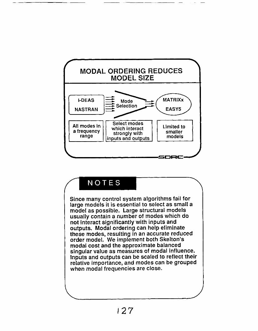
MODAL ORDERING REDUCES
All modes in I a frequency 1 range
Selection
which interact strongly with
Limited to smaller models
Since many control system algorithms fail for large models it is essential to select as small a model as possible. Large structural models usually contain a number of modes which do not interact significantly with inputs and outputs. Modal ordering can help eliminate these modes, resulting in an accurate reduced order model. We implement both Skelton's modal cost and the approximate balanced singular value as measures of modal influence. Inputs and outputs can be scaled to reflect their relative importance, and modes can be grouped when modal frequencies are close.

f ELEMENT FORCES CAN BE 1 I CALCULATED IN EASY5 OR MATRlXx I
NASTRAN ormal Modes and Static Analyses t
I Forces available without returning to NASTRAN Mode acceleration and mode displacement options
Force Time Histories
Applicable to preliminary studies
Calculating element forces and stresses directly in the control system routine can greatly accele- rate turn around time. We transfer the appro- priate matrices from NASTRAN to let us imple- ment a mode acceleration technique. The mode acceleration formulation adds a static correction term to the standard mode displacement for- mulation which improves accuracy when using truncated mode sets. This approach i s appli- cable to parameter studies, where quick turn around time is paramount.

ELEMENT FORCES CAN BE CALCULATED IN NASTRAN
Transient Structural Analyses
t Any NASTRAN solution can be used - Larger models are feasible
Force Time Applicable to detailed stress analysis
Detailed stress analyses fall into the realm of structural dynamicists. In order to facilitate the direct application of NASTRAN to this problem we extract the structural input forces from the controls routine and write these as NASTRAN bulk data. This allows the structural dynamicist the flexibility to choose any NASTRAN transient technique (including a direct transient) to recover element forces and stresses. This method increases turn around time, but is applicable to a detailed stress analysis after control system parameters have been fixed.

CO-ST-IN TRANSLATES EASY5 AND MATRlXx OUTPUT
NASTRAN EASY5 Bulk Data
MATRlXx CO-ST-IN Output
Universal Files Provide:
Flexible plotting options Data management (SYSTAN)
SDRC
As well as provide input to NASTRAN, other reasons for translating control system output include the requirement for more flexible plotting and data management. By translating time simulation output to I-DEAS Universal file format, we can store functions in a database, facilitating the application of powerful data management and plotting capabilities.

CO-ST-IN IS A TOOL FOR CONTROLJSTRUCTURE INTERACTION
Transfers data between structural dynamic (NASTRAN and I-DEAS) and control system software (EASY5 and MATRIXx).
Uses modal ordering to reduce mohel size.
Data recovery performed directly in controls routine using the more accurate mode acceleration method.
EASY5 and MATRlXx output translated for plotting, data management and NASTRAN data recovery.
SDRC-
CO-ST-IN is simply a tool for transferring data among otherwise incompatible analysis pro- grams. CO-ST-IN tries to be smart in what it transfers by using modal ordering to reduce model size and a mode acceleration technique to recover element forces and stresses directly in the controls routine. Control routine output is translated to I-DEAS Universal file format in order to facilitate data management and plotting.

AGENDA
Quick Overview of CO-ST-IN Program
I *Alternate Modal Representations
( Discussion
The main focus of our investigation has been to determine the best possible structural models to use in controllstructure interaction study. Here we define best to mean those which result in the most accurate closed-loop models while using a minimum number of dynamic states. This in- vestigation has led us to examine the use of alternate (other than normal) modal representa- tions.

FIXED INTERFACE MODES REPRE- SENT EFFECT OF INPUT FORCES
-
Normal modes are calculated on basis of free-free boundary conditions Normal modes do not represent effect of input forces Fixed interface (cantilever, Craig-Bampton) modes result in more accurate closed-loop models Improvement even for "soft" controllers
More pronounced for "stiffer" controllers
The basic problem with normal modes is that they are calculated on the basis of free-free boundary conditions. The result is that these modes poorly represent the local effects of forces and moments applied by control actu- ators at these boundaries. The use of fixed interface modes (sometimes called cantilever or Craig-Bampton modes) can help alleviate this problem by providing an accurate static repre- sentation at the location of control inputs. We have found that the use of fixed interface modes does result in more accurate closed-loop mo- dels, even for control frequencies which lie well below flexible frequencies. For stiffer control- lers the differences are even more pronounced.

' CLOSED-LOOP FREQUENCIES MORE ACCURATE
Normallzed
Frequency 1.0%
Error
0.0
0 20 40 60 90 100
Number of Flexible Modes
One measure of accuracy for the closed-loop model is the accuracy of closed-loop frequen- cies. Normalized error is defined as the dis- tance of the approximate frequency from the exact frequency, divided by the magnitude of the exact frequency. In this case we are exa- mining the accuracy of an alpha joint control frequency as we increase the number of open- loop modes, using either a fixed interface or a normal modes representation. In this case control frequencies are close to an order of magnitude below flexible frequencies and the results are consistent with other models that we've looked at.

CLOSED-LOOP FREQUENCY ( RESPONSE MORE ACCURATE
1 %
10 Frcqucncy (radlscc)
Another measure of accuracy for the closed- loop system is accuracy of the closed-loop frequency response. Here we examine the frequency response from an attitude command about the y-axis (roll) to response about the same axis. Normalized error at each frequency is defined as the distance of the approximate to the exact frequency response, divided by the magnitude of the exact response. Note that both representations are inaccurate at high frequencies (where modes are neglected), but that the fixed interface representation is more accurate at lower frequencies. The control frequency in this case is more than an order of magnitude lower than the flexible frequencies and again the results are consistent with other i models we've examined.

SUMMARY
CO-ST-IN transfers data between NASTRAN, IDEAS, EASY5 and MATRlXx
Modal ordering reduces model size
Mode acceleration data recovery performed in control simulation
Fixed interface modal representations result in more accurate closed-loop models
SDRC
Our work with NASA Lewis is on-going, and we will be continuing to develop methods which facilitate fast and accurate closed-loop struc- tural analyses. We will also continue to place emphasis on the selection of improved struc- tural representations for controllstructure inter- action studies.
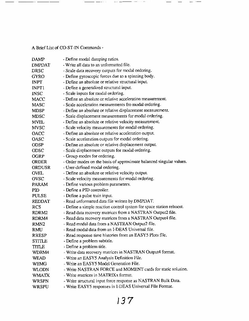
A Brief List of CO-ST-IN Commands -
DAMP DMPDAT DRSC GYRO INPT INPT 1 INSC MACC MASC MDSP MDSC MVEL MVSC OACC OASC ODSP ODSC OGRP ORDER ORDUSR OVEL OVSC PARAM PID PULSE REDDAT RCS RDRM2 RDRM4 RMN2 RMU RRESP STITLE TITLE WDRM4 WEAD WEMG WLODN WMATX WRSPN WRSPU
- Define modal damping ratios. - Write all data to an unformatted file. - Scale data recovery outputs for modal ordering. - Define gyroscopic forces due to a spinning body. - Define an absolute or relative structural input. - Define a generalized stn~ctural input. - Scale inputs for modal ordering. - Define an absolute or relative acceleration measurement. - Scale acceleration measurements fro modal ordering. - Define an absolute or relative displacement measurement. - Scale displacement measurements for modal ordering. - Define an absolute or relative velocity measurement. - Scale velocity measurements for modal ordering. - Define an absolute or relative acceleration output. - Scale acceleration outputs for modal ordering. - Define an absolute or relative displacement output. - Scale displacement outputs for modal ordering. - Group modes for ordering. - Order modes on the basis of approximate balanced singular values. - User-defined modal ordering. - Define an absolute or relative velocity output. - Scale velocity measurements for modal ordering. - Define various problem parameters. - Define a PID controller. - Define a pulse train input. - Read unformatted data file written by DMPDAT. - Define a simple reaction control system for space station reboost. - Read data recovery matrices from a NASTRAN Output2 file. - Read data recovery matrices from a NASTRAN Output4 file. - Read modal data from a NASTRAN Output2 file. - Read modal data from an I-DEAS Universal file. - Read response time histories from an EASY5 Plots file. - Define a problem subtitle. - Define a problem title. - Write data recovery matrices in NASTRAN Output4 format. - Write an EASY5 Analysis Definition File. - Write an EASY5 Model Generation File. - Write NASTRAN FORCE and MOMENT cards for static solution. - Write matrices in MATRIXx format. - Write structural input force response as NASTRAN Bulk Data. - Write EASY5 responses in I-DEAS Universal File Format.

FLEXIBLE MISSIIZ AUTOPILOT DESIGN STUDIES WITH PC-MATLAB/386
Michael J. Ruth Johns Hopklns Unlversity/Applied Physics Laboratory
Laurel, Maryland
ABSTRACT
Development of a responslve. high-bandwidth missile autopilot for airframes which have stmctural modes of unusually low frequency presents a challenging design task. Such systems are viable candidates for modem, state-space control design methods. The PC-MATLAB interactive software package provides an environment well-suited to the developement of candidate linear control laws for flexible missile autopilots. The strengths of MATLAB Include: (1) Exceptionally high speed -- MATLAB'S version for 80386-based PC's offers benchmarks approaching minicomputer and mainframe performance; (2) Ability to handle large desrgn models of several hundred degrees of freedom, If necessary; and (3) Broad extensibility through user-deflned functions. To characterbe MATLAB capabilities, a slmplfied design example is presented. This involves lnteraclive denntlon of an observer-based state-space compensator for a flcxlble missile autopilot design task. MATLAB capabilities and Ilmitations, in the context of this design task, are then surnrnarlirxd.
FREC&DIffi PAGE BLANK NOT FILMED

FLEXIBLE MISSILE AUTOPILOT DESIGN STUDIES W I T H PC-MATLAB/386
Michael J. Ruth Johns Hopkins University / Applied Physics Laboratory
Laurel, Maryland
Workshop on Computational Aspects in the Control of Flexible Systems
12-14 July 1988 Williams burg, Virginia
P R E W M PAGE BUNK NOT FILMED
PRESENTATION OVERVIEW
I. Introduction
2. MATLAB Background
3. Characteristics of MATLAB Environment
4. Classical Control Capabilities
5. Modern Control Design Example
6. Summary

INTRODUCTION
JHUIAPL acts as technical direction agent for US Navy weapon system programs
A key task o f APL's Guidance, Control, and Navigation Systems Group is the evaluation or conceptual design o f missile guidance and control systems
Analysis and design work requires a flexible, j- linear modeling too l
PC-MATLAB resident on 80386 engineering work- stations provides such a too l
W o r k presented here shows general attributes o f M A T L A B , demonstrating use o f PC-MATLAB/386 'for linear design o f a flexible missile autopilot

MATLAB BACKGROUND
M A T L A B (MATrix LABoratory) provides an interactive, matrix-oriented environment
8 M A T L A B is based on the EISPACK and LINPACK routines for matrix computations
8 PC-MATLAB/386 is a high-performance M A T L A B implementation for 80386-based workstations
M A T L A B built-in functions, plus higher-level functions developed for control system calcula- tions, allow for effective controls design studies

HARDWARE AND SOFTWARE CONFIGURATION
COMPAQ 386/20 computer
Weitek 1167 numeric coprocessor
PC-MATLAB1386 with Control Systems Toolbox

PC-MATLAB/386 ATTRIBUTES
Interactive, high-level command environment
Very high processing speed
Easy extensibility via user-defined functions

A M A T L A B INTERACTIVE C O M M A N D LINE EXAMPLE
>> k = Iqr(a,b.q.rho*r); eig(a-b*k), y = step(a-b* k,b.c,d,l,t); p lot (t.y);
The ~ i n n l e line above, typed a t the M A T L A B command line prompt, does several things:
- Computes a quadratic regulator gain vector
- Displays the closed-loop eigenvalues -- often useful for confirming that actuator band- w id th requirements are no t excessive
- Computes and plots a unit step response
By varying the control cost (rho) above, a very large family o f compensators may quickly be considered
The above command line suggests the power and ut i l i ty available f rom a high-level, inter- active matrix language

PC-MATLAB1386 PROCESSING SPEED
MATLAB's UNPACK Benchmark: 460 double precision KFLOPS
This processing speed is:
- 25 x faster than standard PC/AT - 6 x faster than Mac II - 3 x faster than MicroVax II
Implication: the fast response time resulting from such performance allows for truly interactive design iterations on complex control laws

M A T L A B EXTENSIBIL ITY
User-defined functions may be developed through creation of simple text files
Some typical user-defined functions:
- Frequency-response plotting routines
- Application-specific linear transformations
- Multivariable Nyquist criterion
Complex state-space or transfer-function models also defined through user text files

AN EXAMPLE OF A USER-DEFINED C O M M A N D FILE
Below command set calculates and plots the maximum and minimum singular values of a plant and observer-based compensator, for a loop broken at plant input
function [smin,smax] = svdinput(a,b,c,kcon,kobs,w); X jay = sqrt(-1); [nn,xx]=siae(a); i2=eye(nn); [ng,xx]=size(c*a*b); phi = '(s*i2-a)'; for i = 1:nc;
s = w(i)*jay; phieval-+ eval(phi); gs = c/phieval*b; ks - kcon / (phieval+b*kcon+kobs*c) * kobs; xx=avd(ks*g8); smin(i)=xx(ng); smax(i)=u(l);
end ; x x X convert to decibels and plot output X smin=20*loglO(smin); 8m~x=2~*lo#lO(smax); semilogx(w,mmin,w,smax, r-- ) ; grid; title('Hax and Min Singular Values; Loop Broken at Plant Input ' 1 ; xlabel('Frequency (rad/sec)'); ylabel('Mapnitude (db)');
Procedure requires only eleven lines of executable MATLAB code

CLASSICAL CONTROL CAPABILITIES
Frequency response
¤ Root locus
Nyquist plots
Development of dynamic compensators (lead-lag, notch filters, etc)

MODERN CONTROL DESIGN EXAMPLE
Design plant describes tactical missile a t a high-altitude fl ight condition
Design plant includes single-plane rigid- body dynamics and effect o f f irst flexible mode on sensed pitch rate
Objective is t o develop an autopilot t o track commanded accelerations
Design challenge is to achieve high closed-loop bandwidth in presence o f low-frequency bending modes

DESIGN APPROACH
Establish design goals for closed-loop responsiveness and stability
Develop full-state feedback (LQR) gains for design plant
Define linear observer to reconstruct full state vector
- Use "robust observer" design (Doyle and Stein, 1979 IEEE Transactions on Automatic Control)
- Adjust observer gains to recover original LQR loop transfer in desired frequency range

DESIGN PLANT MODEL
Fifth-order state vector g: = h + hu
First three state variables are associated with rigid-body airframe; the last two describe flexible mode dynamics
Rate gyro measurement: [I 0 0 0 11 * g
(Integrated) accelerometer measurement: (0 0 1 0 01 *

SOME OBSERVATIONS ON DESIGN P L A N T MODEL
Feedback o f the first three states describes a very standard (rigid-body) autopilot topology, used by tactical missiles since 1950's
Open-loop plant is characterized by lightly damped airframe (weathercock) poles, and by bending mode poles
- Airframe pole frequency lies a t nominal 2.5 H z
- Bending mode has nominal 25 Hz natural frequency
Desired autopilot crossover frequency here will lie near the bending mode frequency

EFFECT OF STRUCTURAL MODE ON SENSED PITCH RATE (RATE GYRO MEASUREMENT)
Response to Unit Fin Deflection 2 5

CONTROLLABILITY AND OBSERVABILITY PROPERTIES OF P L A N T
System (A&) is controllable
System is unobservable if rate gyro alone, or accelerometer alone, is used as the measurement t o reconstruct state vector
B o t h sensor outputs thus should be used in the observer design
Approach taken for this application:
- Define a (non-square) design plant having one input (fin deflection) and t w o inde- pendent outputs (gyro and accelerometer)
- Use extensions o f loop transfer recovery (Williams and Madiwale, 1985 ACC) valid for non-square systems

FREQUENCY RESPONSE OF FULL-STATE FEEDBACK (LQR) SYSTEM (LOOP BROKEN AT PLANT INPUT)
10-1 1 00 101 102 1 03 104 105
Frequency (rad/sec)

OBSERVATIONS ON LOOP TRANSFER RECOVERY PROCEDURE
For this application, recovery a t b o t h the (rigid-body) airframe and bending mode frequencies may only be achieved with very high observer gains
For practical ranges o f observer gains, recovery a t airframe frequencies is obtained a t the cost o f lessened robustness in the structural mode frequency range
Use o f a set o f user-defined MATLAB files, to implement a range o f observer gain calcu- lations, makes evaluation o f this robustness tradeoff straightforward

RECOVERY OF DESIRED FULL-STATE FEEDBACK SYSTEM WITH MODEL-BASED COMPENSATOR
Frequency (rad/sec)
Asymptotic Loop Transfer Recovery Properties of Compensator 100 - , , , , , , , ,, , , , , , , , , , , , , ,,,, , , , ,
h
P a - 0 - -__-_----- . . . . . . .-
Q, '0 3 4 .-
- 5 0 - m E
-100
-150
. . -.. '. . . . . '.. '. '. . - \ .. '. .*, '.. - ', - - .. .. '. .. .. . . ' . . . . .. * . I. -'. -
1 , 1 1 1 1 , 1 1 I 1 , ,,,, , 1 1 , ,,,,, , , ,I '-. I I , , I,,,, , , , I I , k
10-1 100 101 102 1 03 104 105

ACCELERATION STEP RESPONSE OF FINAL COMPENSATOR DESIGN
Time (sec)

RESPONSE OF FLEXIBLE MODE STATE DURING ACCELERATION STEP RESPONSE
Time (sec)
Pitch Rate Response Due to Flexible Mode 0.5 I 7
0.4
0.3
- -
- -

ACCELERATION STEP RESPONSE FOR CASE WHEN BENDING MODE IS PERTURBED TO 25 % LOWER VALUE
Response to 1-Gee Acceleration Command 1.2
-
-
-
-
-
-0.2 I
0 0.1 0.2 0.3 0.4 0.5 0.6 0.7 0.8 0.9 1
Time (sec)
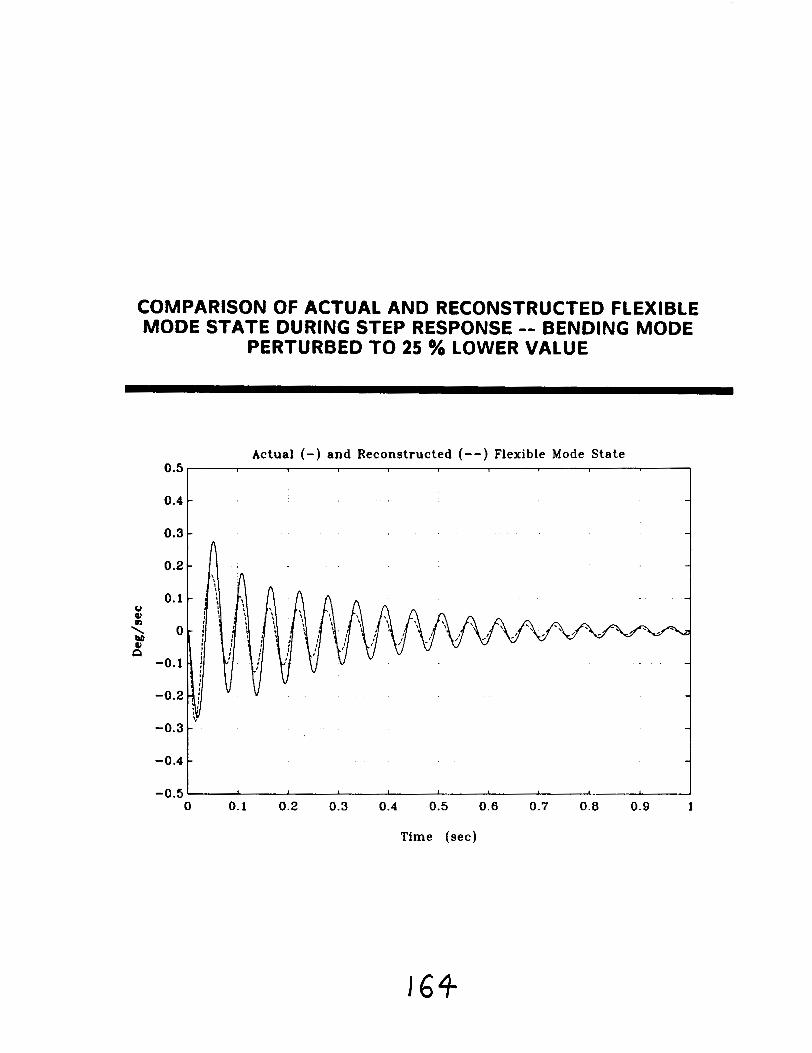
COMPARISON OF ACTUAL AND RECONSTRUCTED FLEXIBLE MODE STATE DURING STEP RESPONSE -- BENDING MODE
PERTURBED TO 25 % LOWER VALUE
Time (sec)
Actual (-) and Reconstructed (--) Flexible Mode State 0.5
0.4
0.3
- -
- A
-
0.2 - -
-
-0.3
-0.4
-0.5
- -
- -
0 0.1 0.2 0.3 0.4 0.5 0.6 0.7 0.8 0.9 1

S U M M A R Y OF DESIGN RESULTS
Model-based compensator yields a high-bandwidth autopilot, which i s robust to a t least a 25% perturbation in bending mode frequency
A number of issues st i l l no t addressed:
- Detailed noise sensitivity assessment - Effect o f higher-frequency structural modes - Phase lag f rom actuator dynamics - Effect of structural modes on accelerometer
measurement - Tolerance to uncertainties in aerodynamics
Above concerns could also be addressed using MATLAB

SUMMARY: MATLAB APPLICABILITY FOR CONTROL DESIGN OF FLEXIBLE SYSTEMS
MATLAB provides the necessary tools for a variety of control system design techniques
Extensibility of MATLAB allows development of tools to implement recent modern control design methods, including loop transfer recovery
Implementation for 80386-based machines (PC- MATLAB/386) has very high performance, allowing for interactive control design of complex systems such as flexible structures
Any flexible structures control problem which can be cast into a state-space framework may benefit from design work with MATLAB

DYSCO - A SOFTIRARE SYSTEM FOR MODELING GENERAL DYNAMIC SYSTEMS
Alex Berman Kaman Aerospace Corporation
Bloomfield. Connecticut
ABSTRACT
The DYSCO program has been under development since 1979. It has been funded by Army and Air Force laboratories and by the Kaman Aerospace Corporation. It is presently available at a number of government and nongovernrnent installations. It has been used to analyze a very broad range of dynamics problems.
A principle feature of the soRware design of DYSCO Is the separation of the executive from the technology. The executive, which controls all the operations. is "intelligent" in the sense that it "knows" that its function is to assemble daerential equations and to prepare them for solution. The "technology l i b rq" contains FORIRW routines whlch perform standard functions. such as. computing the equation coe!Tkients of an element (or "component") given the local state at any tlme. The technology lfbrary also contalns algorllhms and procedures for solving the coupled system equations.
The syslem was deslgned to allow easy additional of technology to the library. Any linear or nonlinear structural entlty, control system, or set of ordlnary dmerential equalions may be simply coded and added to the library. as well as algorithms for time or frequency domain solution.
. ,- The program u&& described wllh emphasis on its usefulness ln easily modeling unusual concepts and configurations. performing analysts of damage. evaluating new algorithms. and slmulallng dynamic tests. Illustrations of several typlcal and illustrative applications presented. A summary of the technology presently residing in the technoloWTaries at the vamus sites +olsDbc glven.
/ *.
1 ' . <

KAMAN AEROSPACE CORPORATION
DYSCO - A SOFTWARE SYSTEM FOR MODELING GENERAL DYNAMIC SYSTEMS
ALEX BERMAN KAMAN AEROSPACE CORPORATION
WORKSHOP ON COMPUTATIONAL ASPECTS I N THE CONTROL OF F L E X I B L E SYSTEMS WILLIAMSBURG, V I R G I N I A , JULY 12-14, 1988

KAMAN AEROSPACE CORPORATION
INTRODUCTION TO DYSCO
o DYNAMIC SYSTEM COUPLER (DYSCO)
o I N I T I A L DEVELOPMENT - 1979
o FUNDED BY ARMY, A I R FORCE, KAMAN
o PRESENTLY OPERATIONAL ON I B M AND VAX
o S I Z E - 50000+ L I N E S OF CODE 350+ SUBROUTINES 4+ MEGABYTES OF STORAGE

KAMAN AEROSPACE CORPORATION
DEFINIT ION OF DOMAIN OF DYSCO
DYSCO COUPLES AND SOLVES SECOND ORDER ODE
. . o MIX, + C,XI + KIX, = F, (COMPONENT I)
o MsXs + CsXs + KsXs = Fs (SYSTEM)

KAMAN AEROSPACE CORPORATION I
DEF IN IT ION OF COMPONENT
o "COMPONENT" I S MORE GENERAL THAN " F I N I T E ELEMENT"
o MI, C,, K,, F, = ARBITRARY FUNCTIONS OF STATE
o X, = ANY GENERALIZED DOF - PHYSICAL, MODAL, OTHER
0 - COMPONENT MAY BE
-4 - - F I N I T E ELEMENT I ASSEMBLY OF F I N I T E ELEMENTS (SUBSYSTEM, OUTPUT OF FE
ANALYSIS) - SPECIAL SET OF EQUATIONS (E.G. , HELICOPTER ROTOR, SPECIAL MECHANISM) - CONTROL ALGORITHM (MIMO, NON-SYMMETRICAL MATRICES, NONLINEAR) - FORCE ALGORITHM (M, C, K = NULL, AERO, ELECTROMAGNETIC)
- ETC., ETC.

KAMAN AEROSPACE CORPORA1 ION
DEFINIT ION OF MODEL
o A MODEL I S A DESCRIPTION OF A COUPLED SET OF COMPONENT EQUATIONS
o COMPONENT EQUATIONS ARE DEFINED BY - 4
- NAME OF THE ALGORITHM I N "TECWNOLOGY LIBRARY"
N - NAME OF DATA SET I N "MODELING DATABASE"
o COMMAND "RUN" COUPLES EQUATIONS
o NEXT STEP I S TO SPECIFY SOLUTION ALGORITHM

KAMAN AEROSPACE CORPORATION
I L L U S T R A T I V E MODEL
COMPONENT 1 CTR4 2 CTR4 3 CTR4 4 CTR4 5 CTR4 6 CTR4 7 C S F l 8 C S F l 9 C S F l 10 C L C l
NO. PATA S E T 1 ABCDl 3 ABCDl 5 ABCDl 2 ABCD2 4 ABCD2 6 ABCD2
TOPR TOPL CONTR GROUND

KAMAN AEROSPACE CORPORATION
DYSCO SYSTEM OVERVIEW
MODELING DATABASE s
- 4
USER


KAMAN AEROSPACE CORPORATION
STANDARD TECHNICAL MODULES
FUNCTION
INPUT
DEFINITION
COEFFICIENT
ACTIVE
OUTPUT
LOADS
COMPONENT
C - - - I
C---D
C---C
C---A
N/A
C---L
FORCE
F - - - I
N/A
F---C
F- - -A
N/A
N/A
SOLUTION
S - - - I
N/A
N/A
S---A
S-9-0
N/A

KAMAN AEROSPACE CORPORATION
TECHNICAL MODULES
---I INPUT DEFINIT ION
---D DEFINE DEGREES OF FREEDOM
---c COMPUTE CONSTANT COEFFICIENTS I N EQUATIONS
- - -A COMPUTE NON-CONSTANT COEFFICIENTS, FUNCTION OF TIME AND STATE
---0 OUTPUT
---L INTERNAL LOADS, FUNCTION OF STATE

KAMAW AEROSPACE CORPORATION
RELATIONSHIP BETWEEN MODELING SCENARIO AND TECHNICAL MODULES
MODELING TECHNICAL MODULES
USER INPUT PROCESS COMPONENT FORCE SOLUTl ON
DEFINE - - - . INPUT COMPONENT
DEFINE - - - - - - - - - - - - - - FORCE
CULAR COMP. FORCES
DEFINE MODEL
COUPLED SYSTEM
EXECUTE I SOLUTION I---.

KAMAN AEROSPACE CORPORATION
RUN COMMAND (ASSEMBLY OF MODEL)
USER INPUT EXECUTIVE FUNCTION TECH. LIBRARY DATA LIBRARY ~ % READ DSIMODEL
MODEL NAME READ DSICOMPONENTS
. ALL I IDENTIFY DOF
I FORM ALL TI AND I
AND
I SYSTEM DOF I
c--- D OF MODEL CONSTRAINTS - i
I
ALL COMPONENTS
OF MODEL
TRANSFORM CONSTANT COEFFICIENTS TO SYS-
TEM MS=MS+TIMIT , . . . L
MIIC,lKIIFI C--- C - - - 1

KAMAW AEROSPACE CORPORATION
T I M E HISTORY SCENARIO (CONTINUATION OF RUN)
USER INPUT EXECUTIVE FUNCTION
1 TECH. LIBRARY
REQUEST SOLUTION INPUT INPUT
T = To
ALL COMPONENTS
OF MODEL
RETRIEVE COMP. STATE I=TIxs(~) \
I I TRANSFORM UPDATED 1 COMP. MI C, K, F , TO SYSTEM AND SUM
I . . SOLVE FOR X ~ ( T )
I INTEGRATE X, TO
XS , XS , T=T+A A -

KAMAN AEROSPACE CORPORATION
FEATURES OF EXECUTIVE
o EXECUTIVE I S SPECIFICALLY BUILT TO MANAGE STRUCTURAL DYNAMIC ANALYSIS
o I T UNDERSTANDS AND MANAGES
- INPUT: IDENTIFICATION, STORAGE, EDITING - MODEL BUILDING: RETRIEVAL OF DATA, CALLS
TO TECHNOLOGY LIBRARY - ASSEMBLY OF EQUATIONS: APPLIES MPC, SPC - SOLUTION OF EQUATIONS: CALLS TO TECHNOLOGY
LIBRARY, RETRIEVAL OF LOCAL STATES, INTERFACE LOADS
o EXECUTIVE INDEPENDENT OF ANY PARTICULAR AREA OF TECHNOLOGY
- UNIFORM ABSTRACT INTERFACES TO TECHNOLOGY LIBRARY

KAMAN AEROSPACE CORPORATION
FEATURES OF TECHNOLOGY LIBRARY
o NEW TECHNOLOGY EASILY ADDED - COMPONENT, FORCE, SOLUTION - UNIFORM INTERFACES TO EXECUTIVE - FORTRAN CODING
o COMPONENTS ARE ANY SECOND ORDER ODE, SUCH AS, - SINGLE SPRING, DAMPER, OR MASS - ANY F I N I T E ELEMENT - COMPLETE NASTRAN MODEL - HELICOPTER ROTOR - MIMO CONTROL ALGORITHM
o SOLUTIONS ACT ON MODEL EQUATIONS, E.G. - EIGENANALYSIS - FREQUENCY RESPONSE - TIME HISTORY - HELICOPTER TRIM (PERIODIC SHOOTING) - PERIODIC SYSTEM STABILITY - STATE FEEDBACK OPTIMIZATION

KAMAN AEROSPACE CORPORATION
OTHER FEATURES
o VALIDATED INPUT AND EDITING - USES KNOWLEDGE TABLE: TYPE, CHARACTERISTICS, EXISTENCE, RANGE - PROMPTED INPUT
- INSTANTANEOUS VALIDATION - ASSURED COMPLETE AND CONSISTENT DATA
b
C;b o SIMPLE EDITING OF MODEL C3 - CONFIGURATION CHANGES
- PARAMETER VARIATION - DAMAGE ANALYSIS
o INTELLIGENT COUPLING PROCEDURES - RECOGNITION OF DOF NAMES - MPC OPTIONALLY AUTOMATICALLY FORMED - GENERAL MPC SOLVED FOR DOF EQUATIONS

KAMAN AEROSPACE CORPORATION
DYSCO BASIC TECHNOLOGY MODULES
o C S F l - LINEAR F I N I T E ELEMENT
USER SUPPLIES: NAMES OF DOF M, C, K, F
o CFM3 - 30 MODAL STRUCTURE
R I G I D BODY, ELASTIC MODES (ALL OPTIONAL) DOF NAMES AUTOMATICALLY GENERATED AUTOMATIC COUPLING AT SPECIFIED NODES
o CSB2 - GENERAL BAR ELEMENT* (NOT AVAILABLE I N GOVT VERSION)
MAY BE USED AS A BEAM OR ROD ELEMENT SHEAR FACTORS, CONSISTENT MASS, RAY LEIGH DAMPING UP TO 12 DOF

KAMAN AEROSPACE CORPORATION
DYSCO BASIC TECHNOLOGY MODULES (CONT'D)
o CESl - ELASTIC STOP
NONLINEAR SPRING, DAMPING, WITH GAP
o CGF2 - GENERAL FORCE
- POLYNOMIAL, FOURIER SERIES, OR TABULAR - PERIODIC
o CLCO - SINGLE POINT CONSTRAINTS
o CLCl - MULTIPOINT CONSTRAINTS
o CLC2 - ADVANCED MULTIPOINT CONSTRAINT
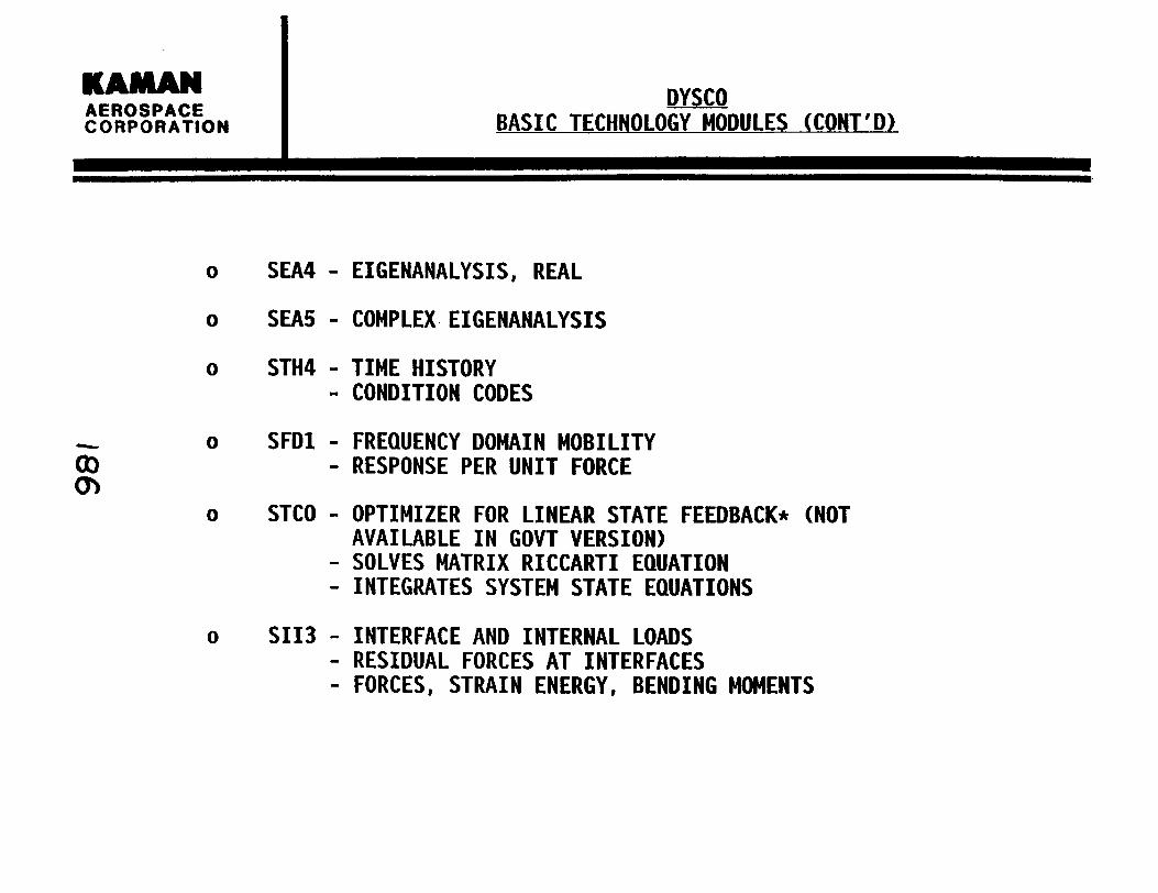
KIMAW AEROSPACE CORPORATION
DYSCO BASIC TECHNOLOGY MODULES (CONT'D)
o SEA4 - EIGENANALYSIS, REAL
o SEA5 - COMPLEX. EIGENANALYSIS
o STH4 - TIME HISTORY - CONDITION CODES
- o SFDl - FREQUENCY DOMAIN MOBILITY - RESPONSE PER UNIT FORCE
o STCO - OPTIMIZER FOR LINEAR STATE FEEDBACK* (NOT AVAILABLE I N GOVT VERSION)
- SOLVES MATRIX RICCARTI EQUATION - INTEGRATES SYSTEM STATE EQUATIONS
o S I 1 3 - INTERFACE AND INTERNAL LOADS - RESIDUAL FORCES AT INTERFACES - FORCES, STRAIN ENERGY, BENDING MOMENTS

KAMAN AEROSPACE CORPORATION
DYSCO - OTHER TECHNOLOGY MODULES
o CRR2, CRR3 - HELICOPTER ROTOR
o CCEO, CCEl - ROTOR CONTROL SYSTEM
o CRD3 - ROTOR DAMAGE
o CFM2 - HELICOPTER FUSELAGE
o CLG2 - NONLINEAR LANDING GEAR
o CLS2 - LIFT ING SURFACE
o FRAO, FRA2, FRA3 - ROTOR AERODYNAMICS
o FFAO, FFC2 - FUSELAGE AERODYNAMICS
o STH3 - TIME HISTORY, HELICOPTER CONTROLS
o STR3 - HELICOPTER TRIM
o SSF3 - FLOQUET STABILITY

KAMAN AEROSPACE CORPORATION
DYSCO AND FE CODES
o DYSCO DOES NOT COMPETE WITH FE CODES
o DYSCO COMPLEMENTS FE CODES
o FE ANALYSIS FOR DETAILED STRUCTURAL ANALYSIS
o DYSCO CAN START WITH FE MODEL AND:
- MODIFY CONFIGURATION - SIMULATE DAMAGE - ADD CONTROL ALGORITHMS - ADD SPECIAL COMPONENTS - PERFORM SOLUTIONS ON ALL MODIFICATIONS - STUDY EFFECTS OF CHANGE - ANALYZE CONFIGURATIONS NOT POSSIBLE (OR
CONVENIENT) WITH FE CODES
o DYSCO CAN ALSO MODEL STRUCTURES ON I T S OWN

KAMAN AEROSPACE CORPORATION
WHAT DYSCO CAN DO FOR YOU
o SIMPLE PROBLEMS ARE EASY AND INEXPENSIVE TO SOLVE
o PROBLEMS NOT CONVENIENTLY MODELED ELSEWHERE CAN BE SOLVED
o PHENOMENA CAN BE BETTER UNDERSTOOD: - - START WITH SIMPLE REPRESENTATION - 00 GRADUALLY INCREASE COMPLEXITY - -4
VARY PARAMETERS - VARY CONFIGURATION
o NOVEL CONCEPTS CAN BE EASILY MODELED AND EVALUATED I
o NEW ALGORITHMS CAN BE TESTED AND EVALUATED I
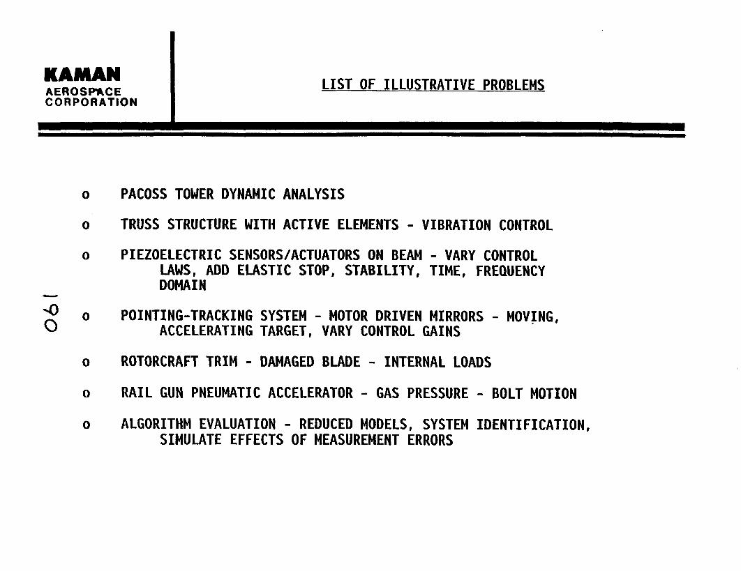
KAMAN AEROSPACE CORPORATION
L I S T OF ILLUSTRATIVE PROBLEMS
PACOSS TOWER DYNAMIC ANALYSIS
TRUSS STRUCTURE WITH ACTIVE ELEMENTS - VIBRATION CONTROL
PIEZOELECTRIC SENSORS/ACTUATORS ON BEAM - VARY CONTROL LAWS, ADD ELASTIC STOP, STABILITY, TIME, FREQUENCY DOMAIN
POINTING-TRACKING SYSTEM - MOTOR DRIVEN MIRRORS - MOVING, ACCELERATING TARGET, VARY CONTROL GAINS
ROTORCRAFT TRIM - DAMAGED BLADE - INTERNAL LOADS
R A I L GUN PNEUMATIC ACCELERATOR - GAS PRESSURE - BOLT MOTION
ALGORITHM EVALUATION - REDUCED MODELS, SYSTEM IDENTIFICATION, SIMULATE EFFECTS OF MEASUREMENT ERRORS

KAMIW AEROSPACE CORPORATION
DYSCO MODELING
o DYSCO COUPLES THE EQUATIONS OF INDIVIDUAL COMPONENTS TO FORM THE EQUATIONS OF A MODEL
o EACH COMPONENT AND MODEL ARE OF THE FORM
o M, C, K, F MAY BE ARBITRARY FUNCTIONS OF TIME OR STATE
o X MAY REPRESENT PHYSICAL, MODAL, OR ANY GENERALIZED DOF
o EACH COMPONENT I S REPRESENTED BY FORTRAN SUBROUTINES I N THE TECHNOLOGY LIBRARY

KAMAN AEROSPACE CORPORATION
COUPLING
o DYSCO USES AN "INTELLIGENT" PROCEDURE FOR COUPLING DEGREES OF FREEDOM
o DEGREES OF FREEDOM OF COMPONENTS MAY BE: - PHYSICAL COORDINATES - MODAL DISPLACEMENTS - ANY GENERALIZED COORDINATES
o COUPLING INCLUDES - PHYSICAL TO PHYSICAL - PHYSICAL TO MODAL - MODAL TO MODAL - SINGLE POINT CONSTRAINTS - MULTIPLE POINT CONSTRAINTS - ANY LINEAR RELATIONSHIPS
o EFFECTS SIMULATED I RIGID PHYSICAL LINKAGES - OPTICAL BEAM COORDINATES - CONTROL ALGORITHMS

KAMAN AEROSPACE CORPORATION
X, XI ARE VECTORS OF THE DOFs OF THE SYSTEM (MODEL) AND THE COMPONENTS
TI I S A TRANSFORMATION MATRIX
THE EQUATION OF THE MODEL I S
WHERE
K = E T;K, T
F = 1 T; F,
EACH T, I S AUTOMATICALLY FORMED I N DYSCO

KAMAN AEROSPACE CORPORATION
COUPLING BY NAME
o DYSCO USES A UNIQUE PROCEDURE WHERE VARIABLE NAMES (A4, 14) ARE RECOGNIZED AND PROCESSED
o NAMES ARE AUTOMATICALLY FORMED OR USER SUPPLIED
o L I K E NAMES I N COMPONENTS IMPLY CONNECTION
o SIMPLE EXAMPLE: X 1 X2 X3 X4
TO CONSTRAIN X3 TO GROUND BY A SPRING, K, USER SIMPLY ADDS COMPONENT TO MODEL WITH FOLLOWING INFORMATION
NO OF DOF = 1 NAME = X3 M = C = F = NULL K = K

KAMAW AEROSPACE CORPORATION
SIMPLE CONTROL SYSTEM EXAMPLE
SENSOR LOCATIONS X I , X4, X 6 ACTUATOR LOCATIONS X3, X 4
F ~ 3 A * X I + B * X ~ + c * X 6 + D * X ~
FX4 = E * X ~ + F * X ~ + c * X 6
T H I S MAY BE REPRESENTED BY COMPONENT WITH
DOF = CX1, X3 , X4, X61
0 0 0 0 C = - 0 0 D 0
E O O G 0 0 0 0
K = - 0 0 0 0 A O B C O O O F 0 0 0 0
SENSOR AND ACTUATOR LOCATIONS MAY BE CHANGED BY E D I T I N G DOF NAMES. GAINS MAY BE CHANGED BY E D I T I N G MATRICES.

KAMAN AEROSPACE CORPORATION
o COUPLING MAY ALSO USE OPTIONAL LINEAR RELATIONS
o SINGLE POINT, MULTIPOINT, CONNECTIVITY CONSTRAINTS
o REPRESENTATION OF MECHANICAL LINKAGES
o CONVERSION TO CONVENIENT PARAMETERS - OPTICAL BEAM ANGLE AS FUNCTION OF MIRROR DOF - T I P DISPLACEMENT OF BEAM AS FUNCTION OF MODAL DOF

KAMAN AEROSPACE CORPORATION
DYSCO I S A DOMAIN EXECUTIVE CONTROL SYSTEM
THE DOMAIN I S "COUPLED DYNAMIC EQUATIONS"
I T EXECUTES TECHNICAL MODULES I N "PARALLEL" (RATHER THAN I N SEQUENCE)
SIMPLE COMMANDS PERFORM NUMEROUS MODULE EXECUTIONS (E. G. , RUN)
INVALID COMMAND SEQUENCES ARE NOT ACCEPTED INVALID DATA USAGE I S NOT POSSIBLE
ALL DATA PLACED ON F ILES OR EDITED I S ASSURED TO BE VALID (E . G . , CONSISTENCY AND FORMAT)

KIMAW AEROSPACE CORPORATION
TERMINOLOGY
o COMPONENT - ALGORITHM FOR COMPUTING MI C, K, F FOUND I N TECHNOLOGY LIBRARY
NAME: C---
o DATA SET - SPECIFIC SET OF DATA TO BE USED WITH A COMPONENT FOUND I N DATA LIBRARY. INPUT BY USER. USER SUPPLIES DATA SET "NAME"
- o MODEL - COLLECTION OF COMPONENTS AND ASSOCIATED DATA SETS
COMPONENT CSF l CSF l CFM2 CSF l CESl
SAMPLE MODEL DATA SET STRUT1 STRUT2 FUSELAGE CONTROL 3 KlOO


* ,* .* x
.* x
* .* .* %
:* * x
.u * Ir .. * * *
3 *
3 *
+ f
9 3
J*
3 3
3%
+
+ 3
*
!*# 'rl
3 *
Q
3
3s
9 3
3*
Q
9'4
-
n
3
Q'r
19
*
3 33
*

KAMAN AEROSPACE CORPORATION
HELIUMl/CAGl HELIUM ACCUMULATOR FOR ET1 MODEL
I I E L I U M ACCUHULATOR FOR E T 1 HODEL
**********************************it****************************n****~*
INF'U'T FOR COMF'ONE).(S CAGf . A D I A B A ' T I C GAS
1 NCDF - NUMBER OF DOF a 3 2 C D F L I - ( D O F ) DOF N A H E
Y K O J I O O O B O L T f O O O M A C Z I O O O 3 GVECT - ( R E A L ) I N I T I A L GAS VECTOR
J . S 5 0 0 0 E + 0 3 4 . 0 0 0 0 0 E + Q Q 1 . 6 5 7 0 0 E + 0 0 2 . 0 7 ' 7 0 3 5 + 0 0 0 . 4 0 0 8 0 E + 0 4
4 AREA - ( R E A L ) M A T R I X FOR AREA C A L C GENERAL HA1'R I X
ROW 1 '
2 . 0 0 0 0 0 E + 0 0 2 . 0 0 0 0 0 E + 0 0 3 . 0 0 0 0 0 E + 0 0
ROW 2 I .OOOOOE+00 \ .OOOOQE+00 6.66670E-01
5 GOVDOF - ( D O F ) AREA E X I S T C R I T E R I A PRO J I 000 B O L T 1 800 B O L T 1 0 0 0
6 AECV - ( R E A L ) GOVDOF C R I T I C A L V A L U - 1 . 0 0 0 0 0 € + 0 4 - 1 . 0 0 0 0 0 E + Q 4 1 . 0 0 0 0 0 E + 0 0
'7 PECDOF - PRESSURE EX C R I T E R I A = PRO J 1 000 (3 F' f iCVhL -- C R I I ' I C A L V A L U E = 7 . 7 5 0 0 0 E + 0 0
n n ~ # ~ * W % * * # # * % S Y t i t * * 1 ( * * t i t i t * Y * * * * i t S * * S * * * ~ * * * * N ~ * * ~ * * M * * ~ # ~ N % U ~ * N S ~ M W * * ~

KAMAN AEROSPACE CORPORATION
PYSCO LIBRARIES
o TECHNOLOGY LIBRARY CONTAINS
COMPONENT REPRESENTATIONS (C . . . 1 FORCE ALGORITHMS (F . . . 1 SOLUTION ALGORITHMS (S ... 1
o DATA LIBRARIES CONTAIN
DATA ASSOCIATED WITH PARTICULAR C ..., F ... AND IDENTIFIED BY DATA SET NAME SUPPLIED BY USER
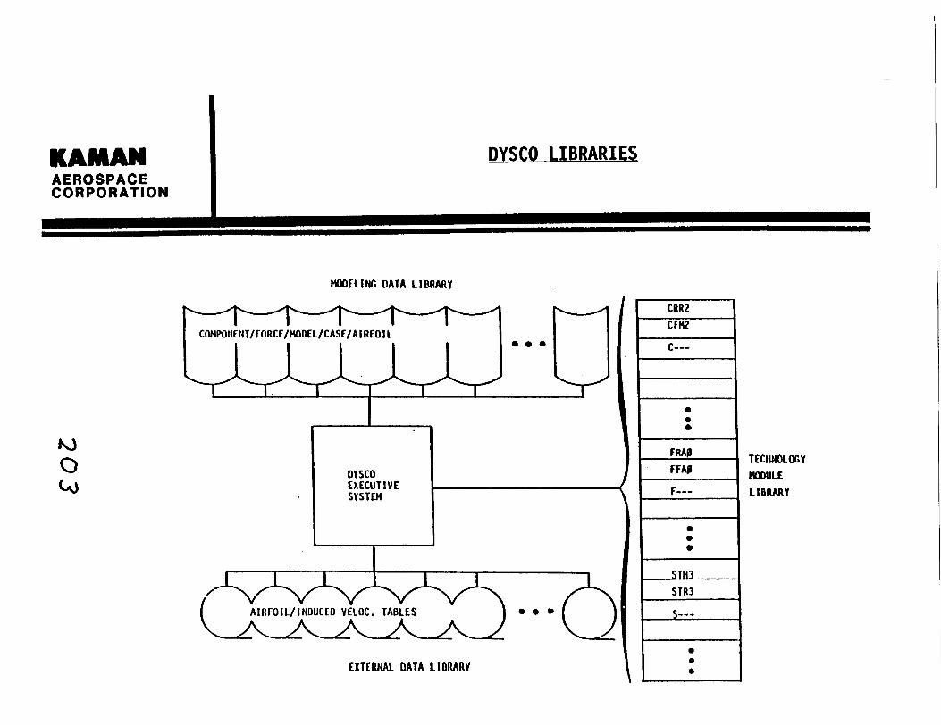
AEROSPACE CORPORATION
DYSCO L I B R A R I E S
HODEL I NC DATA LIBRARY
EXTERNAL DATA L 1 ORARY \
TECtiNOLOGY HOOULE
LIBRARY

KAMAN AEROSPACE CORPORATION
TECHNOLOGY LIBRARY
ANY TECHNOLOGY MODULE MAY BE ADDED TO LIBRARY I F :
COMPONENT, FORCE
M, C, K, F MAY BE COMPUTED AS FUNCTIONS OF LOCAL STATE VECTOR AND T IME BY A FORTRAN PROGRAM
SOLUTION
ALGORITHM MAY BE WRITTEN I N FORTRAN, GIVEN SYSTEM M, C, K, F, AS ABOVE

KAMAN AEROSPACE CORPORATION
TYPICAL COMMANDS
COMMAND
NEW ALLOWS USER TO MODIFY MODEL ALLOWS USER TO CREATE NEW COMPONENT/FORCE INPUT DATA
u RERUN NEW SOLUTION FOR MODEL JUST RUN
0 (rl
RUN FORMS EQUATIONS OF MODEL AND EXECUTES A SOLUTION
EDIT ALLOWS USER TO TO MODIFY MODEL AND PERFORM VALIDATED EDIT OF INPUT DATA

KAMAN AEROSPACE CORPORATION
ABSTRACT BASIS OF DYSCO
DYSCO ACHIEVES I T S MULTIPURPOSE CAPABILITY BY A COMPLETE SEPARATION OF ABSTRACT AND SPECIFIC DATA.
SINCE DYSCO DOES NOT TREAT SPECIFIC PHYSICAL COMPO- NENTS, FORCES, OR SOLUTIONS, I T CAN SOLVE PROBLEMS INVOLVING ANY COMPONENTS, FORCES, OR SOLUTIONS.

KAMAN AEROSPACE CORPORATION
USER'S APPROACH TO DYSCO ANALYSIS
THE USER PERCEIVES A "MODEL" MADE UP OF COMPONENTS
HE THEN:
SELECTS APPROPRIATE REPRESENTATIONS FOR EACH COMPONENT FROM THE LIBRARY
SELECTS APPROPRIATE FORCE ALGORITHMS FOR EACH COMPONENT
u 0 SELECTS APPROPRIATE SOLUTION METHODS.
NOTE THAT THE ORIGINAL MODEL FORMULATION REQUIRES AN APPROPRIATE LEVEL OF ENGINEERING JUDGEMENT.
FOR EACH COMPONENT AND FORCE, THE DATA MUST BE IDENTIFIED AS RESIDING ON A USER F I L E OR THE DATA MUST BE PLACED ON A F I L E USING DYSCO.
THE MODEL AND VARIATIONS MAY THEN BE FORMED INTERACTIVELY AND SPECI- FIED SOLUTIONS MAY BE CARRIED OUT.

KAMAN AEROSPACE CORPORATION I
ILLUSTRATIVE APPLICATIONS

KAMAN AEROSPACE CORPORATION
DYSCO 2D STRUCTURAL MODEL
MOTOR
.UYa
BASE 2)-M
MODEL 1 18 DOF (GROUNDED) 2-5 VARIOUS BASE SHAKES 6 2 1 DOF (3 BASE DOF)

KIMIW AEROSPACE CORPORATION
CONTROL GAINS
I. MAX TORQUE FOR MOTOR AT MAX RATE .05 R/S - 3 7 0 I N #
11. DESIGN TORQUE T = 185 I N #
111. I N I T I A L TRIAL GAINS
1. DISPLACEMENT GAIN I F t$ I S AT A MAX ALLOWABLE ERROR OF 15 p ~ , LET MOTOR BE DRIVEN AT MAX SPEED
2. VELOCITY GAIN
I F i I S AT MAX RECESSION OR APPROACH OF . 0 5 ~ l s , LET MOTOR BE DRIVEN AT MAX SPEED

KAMAN AEROSPACE CORPORATION
TYPICAL STRUCTURAL VARIABLES MONITORED
I. MIRROR AND MOTOR
1. THET9 = e = TARGET L. 0. S. FROM INERTIAL REFERENCE
2. DSTRl = a * = ACTUAL DRIVE ANGLE OF MIRROR
3. MTHl = O M = STRUCTURAL VIBRATION OF THE MOTOR MOUNT
4. 26* + O M = OX' (BENT OPTICAL AXIS) FROM I N E R T I A L REFERENCE
6* DSTRl NEWTONIAN REFERENCE --fS+=~$=5~1~ OX' rat
TARGET -

KAMAW AEROSPACE CORPORATION
CASE 1 T I M E HISTORY (PAGE 1 OF 3)
CASE 1 TIUE HISTWY STATIONARY TARGET AT ZEl# ---- INITIAL WISPOINl DSTR - 15 rrad
w INITIAL LINES-OF-SIGHT STATI[YWIY COCIlROLS
Solid - Optlcrl Wlrpoht of Flat Mirror DLspl. 6aln = Wax Avail. Val. Gain - Max Avail.

KAMAN AEROSPACE CORPORATION
CASE TIME HISTORY (PAGE 2 OF 3)
CASE 0 TIME HISTORY ACCELERATING TARGET ------- INITIAL MISPOINT. OSTR - i5 firad
KAMAN INITIAL LINES-OF-SI6HT APPfWACHIN6 CONTRQCS
Solid - Target DLspl. 6aln - .&Max Dotted - Pointing Axis L.'O.S. Val. 6ain -.a1 Max

KAMAN AEROSPACE CORPORATION
CASE TIME HISTORY (PAGE 3 OF 3)
CASE 8 TIME HISTORY ACCUEAAT ING TAJYiET --- INITIAL UISWINT OSTA - 15 ,pad m INITIAL LINES-OF -SI6HT APPROAMING CONTR~S:
Solld - Target 0lsp.l. 6aln - .el )(ax Dotted = Orlven Ulrror Angle Val. 6aln - .8 l Max Dashed - kt& Wwnt Response

KAMAN AEROSPACE CORPORATION
R A I L GUN PNEUMATIC PRE-ACCELERATOR
SPRING DETENT
1
I IR -*--C----xq 9 P T R, Y I /- O D O. ' O D
I
I - ' I Po = 4550 p s l
SNUBBER
L 1 I
"1 "2 -. F2 (PRELOAD)
. . - . . %2 -Y
I
(PRELOAD) w Y - 1.667 ( I l e l l l w ) .
x3SNUBBER
rn = P R O J E C T I L E 1 m2 = BREECH BOLT " 3 = MAGAZINE STACK
x2 SNUBBER 4 \ - L x - x3 SNUsBER 2 I I 1 a
a
EQUATION OF MOT IOEI -
-
A3 = 0 UNLESS
x 2 > C BEFORE
PRESSURE VENTS


AEROSPACE CORPORATION
TRADES STUDIES FOR PRE-ACCELERATOR
E T PREACCELERATOR, BEHAVIOR VS. TOTAL MASS AND PERCENT ALLOTTED TO BOLT

KAMAW AEROSPACE CORPORATION
MODEL FOR HARMONIC BOLT RETURN AND IMPACT W I T H FRESHLY LOADED PROJECTILE
C---..--
SPRlWG DLTENT FOR a, 1 '1 I
4 Xz !
- CESl FOI IWACT cw 9 u r n =, F
VARIOUS COEFFICIENTS OF RESTITUTION CAN BE MODELLED BY JUDICIOUS CHOICE OF K AND C
. . . . . . . . . . . . . . . . . . . . . . . . MODEL IMPACT 2 ........................... IMPACT MODEL PLUS BARREL FIT/MAGAZINE FRICTION AND BALL SPRING DETENT
INDEX COMP NO. DATA SET FORCE DATA SET 1 C S F l BRlDYN NONE 2 C E S l BOLT2.0 NONE 3 CSDl BALL2 NONE 4 C D F l IMPMU NONE

KAMAN AEROSPACE CORPORATION
IMPACT DETAI L DISPLACEMENT AND VELOCITY

MODELING AND CONTROL SYSTEM DESIGN AND ANALYSIS TOOLS FOR FLEXIBLE STRUCTURES
Arnir A. Anissipour Russell A. Benson
Edward E. Coleman
The Boelng Company Seattle. Washington
ABSTRACT
Deslgn and analysis of contxpl systems for flexible structures requlre accurate math-7 models of flexible structures and software design wlth the analysls tools capable of 11;lndling these models while mal@ahing numerical accuracy. Since aeroelastic models
4 , ' 01 flexlble structures tend to be laige (e.g., 100 states), the availability of tools to handle such large models is cruchl. Initial model development fs based on aerodynamic rnathematlcal models. wind tunnel data. mathematical structural models, and ground
." ; shake test resulls. E&ntually. flight test data are used to update and reflne the model. - fl' i -. -- Wie paper &wrihes BoeIng software tools used for tlle development of control laws of \
flcxlble structures. i b
Tlie Boelng Company has developed a software tool called Modem Control Software Package (MPAC). MPAC provides the environment necessary for linear model
i I
development. analysis, and controller design for large models of flexible structures. There are two features of MPAC which are particularly approprtate for use wlth large models: (11
I
rlumerical accuracy and (2) label-driven nature. With the first feature MPAC uses double , prcclsion arithmetic for all numerical operations and relles on EISPAC and LINPACK for llie numerical foundation. With the second feature. all MPAC model inputs, outputs, and stales are referenced by user-defined labels. This feature allows model modlllcatlon while nlaintalning the same state. Input. and output names. In addltion, there is no need for the user to keep Crack of a model variable's matrix row and column locations.
There is a wide range of model manipulation. analysis. and design features within the numerically robust and flexlble envlronrnent provided by MPAC. Models can be built or nlodllled using either stale space or transfer function representations. Exlsting models can be combined via parallel, series. and feedback connections; and loops of a closed-loop model may be broken for analysls. Analysis tools available include: elgenvalue/eigenvector. controllability matrix. observability matrix. transfer function generatlon. frequency response and singular value plots, covariance response to white noise or atmospheric turbulence models. model simulatlon using step, sinusoidal. random. or user-defined inpuls. Control system design tools Include: root locus. LQC full slate feedback gain matrix computation, LQG full-order estimator design. and robust low order controller (SANDY) design a s developed by Dr. Uy-Loi Ly at Stanford.

The existing Boelng Company structural analysis and design software package. ATLAS. has been extended in order to form a state-space model for input to MPAC. The new capabllily. a module named DYFORM. is a n outgrowth of earlier work under a NASA contract for Integrated Application of Active Controls. The structural and theoretical aerodynamic mathematical model originates within ATLAS in exactly the same fashlon a s for conventional flutter and dynamlc loads analyses. The DYFORM module is then used to construct the state-variable model a s required by MPAC. Its capabllitles include (1) control surfaces and/or gust vector as Inputs. (21 sensors and/or loads quantilies as outputs. (31 foxmulatlon in body-llxed or inertial axes. (4) modlficatlon of the theoretical aerodynamics using wind tumel/fllght test data from rigid or flextble-model tests. and [5) use of S-plane rational alrloads expressions to formulate the state model Including augmented states to represent unsteady aerodynamfc effects.
MPAC has been used for yaw damper design (including active flexible mode suppression) ol the Boeing 767 and 747 airplanes. The flexible structural models of these planes. as large as 100 states. have been handled by MPAC without loss of numerical accuracy.
The Boelng Company plans for the development of a system identfncation and parameter estlmatlon [SIPEI software tool. The system ldentiflcatlon algorithms employ a multiple stepwise regression technique to determine the structure of the system. The parameter estimatlon algorithms update the current model using maxlmum likelihood estimation. Tlle SIPE routines wffl be compatible with MPAC and RF-DATA (a data correction and reroxmattlng program also developed by Boeing). The SIPE routhes will be flexible. allowing the user to select gradient methods. integration algorithms. and Rlccati solution algorithms. The MPAC compatible model structure slated for the SIPE package will be applicable to any dynamic system. Aerodynamic. aeroelastic. ground effects. and sensor noise modeling will all be possible.

INTRODUCTION TO MPAC:
A Control Law Design Tool Well Suited for
Flexible Structure Applications
Edward E. Coleman
The Boeing Company Boeing Commercial Airplanes
P.O. Box 3707 Seattle, Washington 98124-2207


BOEING COMMERCIAL AIRPLANES GUIDANCE AND CONTROL RESEARCH
MPAC Features:
Label Driven Model Format:
- User defined state, input, and output labels of up to 8 characters.
Numeric Robustness:
- Built on Eispac, LINPACK, and ORCALS - Double precission computation throughout - Handles models up to 256 elements (states, inputs, and outputs)
Modular Structure:
- Each command is a seperate subroutine - User need learn only those comands helshe wants to use - Wide range of available commands - Provission for customized, user defined commands

BOEING COMMERCIAL AIRPLANES GUIDANCE AND CONTROL RESEARCH
Binary Model File
Model File
\ r \ I \ J \ 1
Command \ \ I I 4 / d
\ I f l /
Data
File \ \ I J .) H d File
\ I a #
d /
/
MPAC 1 1
. I \ '.
I \ '. I \ \ .
I \ \
I \ '. \ Binary Output I \ I \
I \ Model
File t \ I \
I
3 \ File L
Graphic Data Output File
Output Model File

BOEING COMMERCIAL AIRPLANES GUIDANCE AND CONTROL RESEARCH

.L COMPUTE THE ASVMPTOTIC POLES OF FULL STATE FEEDBACK GAlN FOR THE reg
COMPUTE THE ASYMPTOTIC POLES OF KALMAN FILTER GAlN FOR THE reg
COMPUTE THE COMPANION MODAL MODEL OF THE reg, replacement-opt~on
COMPUTE THE CONJUGATE MODAL MODEL OF THE reg, replacement-optlon
COMPUTE THE CONTROLLABILITV MATRIX OF THE reg
COMPUTE THE COVARIANCE RESPONSE OF THE reg TO turbulence-model AND covariance-print-option
'. COMPUTE THE COVARIANCE RESPONSE OF THE reg TO WHITE NOISE AND covar~ance-print-optlon Model Properties COMPUTE THE DISCRETE COVARIANCE RESPONSE OF THE reg TO WHITE NOISE AND corar~ance-pr int-opt lon
COMPUTE THE EIGENVALUES OF THE reg
Model M o d ~ f ~ c a t ~ o n COMPUTE THE EIGENVECTORS OF THE reg
COMPUTE THE FREQUENCY RESPONSE OF THE reg
,,,,,,,:Model Reduc t~on COMPUTE THE OBSERVABILITV MATRIX OF THE reg
COMPUTE THE RESIDUES OF THE reg
Model Trans format~on COMPUTE THE ROOT LOCUS OF THE reg
COMPUTE THE SETPOINT MATRICES FOR THE reg
COMPUTE THE SIMILARITY TRANSFORM OF THE STATE MODEL FOR THE reg
COMPUTE THE SINGULAR VALUES OF THE reg
COMPUTE THE TRANSFER FUNCTION(S) OF THE reg
COMPUTE THE TRAFlSMlSSlON ZEROS OF THE reg
CONSTRUCT THE DRVDEFJ TURBULENCE MODEL FOR THE reg
CONSTRUCT THE EQUATIONS OF MOTION FOR THE reg
COPV THE STATE MODEL OF THE reg TO THE des t~na t~on - reg
CREATE STATE ESTIMATOR FOR THE reg
CREATE control ler-type FOR THE reg
CREATE control ler-type FOR THE reg WITH MODEL FOLLOWING
NO. Comments DESIGN THE DISCRETE FSF (FULL STATE FEEDBACK) GAIN MATRIX FOR THE reg
DESIGN THE DISCRETE STATE ESTIMATOR (KALMAN FILTER) GAIN MATRIX FOR THE reg ' 1 I - > DESIGN THE EMF (EXPLICIT MODEL FOLLOWING) G A l l l MATRIX FOR THE reg
2 -' DESIGN THE FSF (FULL STATE FEEDBACK) GAIN MATRIX FOR THE reg
DESIGN THE LTS (LINEAR TRACKING SYSTEM) GAlN MATRIX FOR THE reg 3 - >
DESIGN THE STATE ESTIMATOR (KALMAN FILTER) GAIN MATRIX FOR THE reg
DESIGN ROBUST LOW-ORDER CONTROLLER
BOEING COMMERCIAL AIRPLANES GUIDANCE AND CONTROL RESEARCH

. . . . . . All FdlPiiL Lolnlr~ands ...........................................................................................................................................................................................
DESIGN THE STATE ESTIMATOR (KALMAN FILTER) GAIN MATRIX FOR THE reg
DESIGN ROBUST LOW-ORDER CONTROLLER
DISCONNECT THE CLOSED LOOP OF THE reg
FEEDBACK CONNECTION: a-reg IS CONNECTED TO THE b-reg AND IS PLACED INTO THE destination-reg
FORM THE CLOSED LOOP SYSTEM: CONNECT THE controller-option TO THE CIS-reg
FORM THE pim-reg WlTH THE IDEAL MODEL (AND PLACE IT INTO THE PLANT + IDEAL MODEL)
FORM THE pse-reg WlTH THE estimator-option (AND PLACE IT INTO THE PLANT + STATE ESTIfU1ATOR)
LOAD THE G (FULL STATE FEEDBACK GAIN) MATRIX
LOAD THE S (ESTIMATOR GAIN) MATRIX
LOAD THE STATE MODEL OF THE reg
LOAD transfer-fn-type TRANSFER FUNCTlO N INTO THE reg
MODIFY THE G MATRIX BY modification-method
MODIFY THE S MATRIX BY modification-method
MODIFY THE STATE MODEL OF THE reg
PARALLEL CONNECTION: a-reg IS CONNECTED TO THE b-reg AND IS PLACED INTO THE destlnatlon-reg
PRINT THE G (FULL STATE FEEDBACK GAIN) MATRIX
PRINT THE S (ESTIMATOR GAIN) MATRIX
PRINT THE STATE MODEL OF THE reg
READ THE STATE MODEL FOR THE reg ( IN MATLAB FORMAT)
READ THE STATE MODEL FOR THE reg (MPAC FORMAT)
REDUCE THE ORDER OF THE reduce-reg
RESTORE THE ORIGINAL G MATRIX (AFTER MODIFY COMMAND)
RESTORE THE ORIGINAL S MATRIX (AFTER MODIFY COMMAND)
RUN MATLAB
SERIES CONNECTION: a-reg IS CONNECTED TO THE b-reg AND IS PLACED INTO THE destination-reg
SIMULATE THE LINEAR STATE MODEL OF THE reg
SIMULATE THE LINEAR STATE MODEL OF THE reg WlTH A Its-controller-reg (LINEAR TRACKING SYSTEM)
TRANSFORM reg USING transform-option
WRITE THE STATE MODEL FOR THE reg ( IN MATLAB FORMAT)
WRITE THE STATE MODEL FOR THE reg ( IN EASY5 FORMAT)
WRITE THE STATE MODEL FOR THE reg (MPAC FORMAT)
XXX nopt
BOEING COMMERCIAL AIRPLANES GUIDANCE AND CONTROL RESEARCH

BOEING COMMERCIAL AIRPLANES GUIDANCE AND CONTROL RESEARCH

BOEING COMMERCIAL AIRPLANES GUIDANCE AND CONTROL RESEARCH
This is an example MPAC command file. The output file generated using this command file is given on the following pages.
* W A C READ PLANT LAT2 .MDL
*COMPUTE EIGENVALUES OF PLANT
"DEFINE PLANT DELETE STATE PSI CREATE STATE BETA-1NT.dot: 1. BETA CREATE OUTPUT PHI-CRIT: 1. PHI.dot 5.0 PHI CREATE OUTPUT BETA-CRIT: 1. BETA.dot 3.2 BETA 4 . BETA-INT END
*DESIGN GAIN MATRIX FOR PLANT .001 2' 2 'AIL' 1. ' RUD' 2. ' PHI-CRIT' 4. 'BETA-CRIT' 1. ' WLOCUS ' 'RHO' I., 1.' 1 $ FIRST CUT LATERAL GAIN LOCUS $ AIL=l. RUD=2. $ PHI - CRIT=4. BETA-CRIT=l.
*CREATE CONTROLLER FOR PLANT ' NODIRECT'
*FORM PLANT + CONTROLLER
*PRINT CLOSED-LOOP SYSTEM
*COMPUTE EIGENVALUES OF CLOSED-LOOP SYSTEM
"MPAC WRITE CLOSED-LOOP SYSTEM CLOSED LOOP .MDL -

BOElNG COMMERCIAL AIRPLANES GUIDANCE AND CONTROL RESEARCH
MPAC output file example. Output file generated using command file on previous
MPAC RELEASE VERSION 4 . 0 0 0 5 MAY 1 9 8 7 (CONFIGURATION CONTROL I
*----------------------------- .................... -----==-------- -- --------==------ ------=* * MPAC INPUT/OUTPUT FILE DESCRIPTION * ....................................................... . . . . . . . . . . . . . . . . . . . . . . . . . . . . . . . . . . . . . . . . . . . . . . . . . . . . . . . COMMAND FILE ----------------- example.cmd MODEL FILE ------------------- INPUT BINARY FILE ------------ OUTPUT BINARY FILE ----------- MPAC OUTPUT FILE ------------- example.out W A C GGP PLOT FILE ----------- example.ggp MPAC USER DATA FILE NO.l ----- MPAC USER DATA FILE N0.2 ----- W A C USER-DEFINED UBIN FILE -- TIME OF MPAC JOB EXECUTION --- Tuesday, July 5, 1988 3:50:36 pm (PST)
* * * * * * ****** * * * * * * MODERN CONTROL THEORY ANALYSIS/SYNTHESIS SOFTWARE PACKAGE * * * * * * ****** * * * * * * * * * * * * APOLLO-VERSION: MPAC 4 . 0 0 ON APOLLO FORTRAN 8 . 4 0 * * * * * * * * * * * * * * * * * *
* * * MODEL READ FROM FILE: LAT2.MIL * * * ELAPSED TIME (SEC) : 0 . 2 4

BOEING COMMERCIAL AIRPLANES GUIDANCE AND CONTROL RESEARCH
. . . . . . . . . . . . . . . . . . . . . . . . . . . . . . . . . . . . . . . . . . . . . . . * * * * * * * * * * * * * * * * * * * TASK 2 * * * * * * * * * * A * * * * * * * * *
. . . . . . . . . . . . . . . . . . . . . . . . . . . . . . . . . . . . . . . . . . . . . . . * * * * * * * * * * * * * * * * * * *COMPUTE EIGENVALUES OF PLANT * * * * * * * * * * * * ****** * * * * * * * * * * * * * * * * * * * * * * * * * * * * * * * * * * * * * * * * * A * * * * *
* * * * * * * * * * * * * * * * * * * TASK 2 * * * * * * * * * * * * * * * A * * * *
. . . . . . . . . . . . . . . . . . . . . . . . . . . . . . . . . . . . . . . . . . . . . . .
SAMPLING TIME : DELTA = 0 . 0 0 0 0
COUNT REAL PART IMAG PART DAMPING FREQ (RAD/S) FREQ ( H Z ) ............................................................................
1 0 . 0 0 0 0 0 . 0 0 0 0 0 . 0 0 0 0 0 . 0 0 0 0 0 . 0 0 0 0 2 - 1 . 2 9 8 9 E - 0 2 0 . 0 0 0 0 1 . 0 0 0 1 . 2 9 8 9 E - 0 2 2 . 0 6 7 3 E - 0 3 3 - 0 . 1 4 0 3 1 . 6 7 6 8 .3426E-02 1 . 6 8 2 0 . 2 6 7 7 4 - 0 . 1 4 0 3 - 1 . 6 7 6 8 . 3 4 2 6 E - 0 2 1 . 6 8 2 0 . 2 6 7 7 5 - 1 . 9 4 6 0 . 0 0 0 0 1 . 0 0 0 1 . 9 4 6 0 . 3 0 9 7
ELAPSED TIME (SEC) : 0 . 1 4
DELETED STATE P S I CREATED STATE BETA-INT.: 1 . 0 0 0 CREATED OUTPUT PHI CRIT: 1 . 0 0 0 CREATED OUTPUT BETA CRIT: 1 . 0 0 0
BETA P H I . BETA.
P H I BETA
. . . . . . . . . . . . . . . . . . . . . . . . . . . . . .
ELAPSED TIME (SEC) : 0 . 1 0

BOEING COMMERCIAL AIRPLANES GUIDANCE AND CONTROL RESEARCH
****** *DESIGN GAIN MATRIX FOR PLANT * * * * * * * * * * * * * * * * * *
DESIGN PARAMETERS: ------------------
ALPHA - 1 .00000E-03
CONTROL VARIABLE CONTROL WEIGHT (R) AIL 1 . 0 0 0 0 RUD 2 . 0 0 0 0
CRITERIA VARIABLE CRITERIA WEIGHT (Q) PHI CRIT 4 .0000 BETZ-CRIT 1 . 0 0 0 0
...........................................
----- ----- STEADY STATE RICCATI SOLUTION ===== ------ .........................................
SAMPLING TIME : DELTA = 0 .0000
COUNT REAL PART IMAG PART DAMPING FREQ (RAD/S) FREQ (HZ) ............................................................................ 1 -0 .9492 0 . 0 0 0 0 1 . 0 0 0 0 . 9 4 9 2 0 . 1 5 1 1 2 - 1 . 5 7 4 1 . 4 5 3 0 . 7 3 4 6 2 . 1 4 2 0 . 3 4 0 9 3 - 1 . 5 7 4 -1 .453 0 . 7 3 4 6 2 . 1 4 2 0 . 3 4 0 9 4 - 4 . 4 4 2 2 . 5 3 2 0 . 8 6 8 8 5 . 1 1 3 0 . 8 1 3 8 5 - 4 .442 -2 .532 0 . 8 6 8 8 5 . 1 1 3 0 . 8 1 3 8
................................ ................................ ----- ----- FEEDBACK GAIN MATRIX ===== ................................
BETA P PHI R BETA-INT ............................................................
A 1 L 5 .470 - 2 . 6 0 5 -9 .524 -2 .000 1 . 0 9 3 RUD -3 .065 - 0 . 5 1 2 7 - 2 . 0 5 9 2 . 0 5 6 - 2 . 7 2 2
ELAPSED TIME (SEC) : 1 . 1 7

BOEING COMMERCIAL AIRPLANES GUIDANCE AND CONTROL RESEARCH
* * * * * * * * * * * * * * A * * * * TASK 5 * * * * * A * * * * * * * * * * * * *
. . . . . . . . . . . . . . . . . . . . . . . . . . . . . . . . . . . . . . . . . . . . . . * * * * * * * * * * * * * * * * * * *CREATE CONTROLLER FOR PLANT * * * * * * * * * * * * * * * * * * . . . . . . . . . . . . . . . . . . . . . . . . . . . . . . . . . . . . . . . . . . . . . * * * * * * * * * * * * * * * * * * * TASK 5 * * * * * * * * * * * * * * * * * * * . . . . . . . . . . . . . . . . . . . . . . . . . . . . . . . . . . . . . . . . . . . . . .
" * * * * FULL STATE FEEDBACK CONTROLLER * * * * * * * * * * NO MODEL FOLLOWING * * * * * * * * * * DIRECT F . B . STATES TO PLANT * * * * * BETA P P H I R BETA-INT . . . . . . . . . . . . . . . . . . . . . . . . . . . . . . . . . . . . . . . . . . . . . . . . . . . . . . . . . .
ELAPSED TIME ( S E C ) : 0 . 5 0
. . . . . . . . . . . . . . . . . . . . . . . . . . . . . . . . . . . . . . . . . . * * * * * * * * * *+ * * * * * * TASK 6 * * * * * * * * * * * * * * * * * . . . . . . . . . . . . . . . . . . . . . . . . . . . . . . . . . . . . . . . . . . * * * * * * * * * * * * * * * * * * *FORM PLANT f CONTROLLER * * * * * * * * * * * * * * * * * * . . . . . . . . . . . . . . . . . . . . . . . . . . . . . . . . . . . . . . . . . . * * * * * * * * * * * * * * * * * TASK 6 * * * * * * * * * * * * * * * * * . . . . . . . . . . . . . . . . . . . . . . . . . . . . . . . . . . . . . . . . . .
. . . . . . . . . . . . . . . . . . . . . . . . . . . . . . . . . . . . . . . . . . . . . . . . . . . . . . . . . * * * * * FULL STATE FEEDBACK CONTROLLER * * * * * * * * * * NO MODEL FOLLOWING * * * * * . . . . . . . . . . . . . . . . . . . . . . . . . . . . . . . . . . . . . . . . . . . . . . . . . . . . . . . . .
ELAPSED TIME ( S E C ) : 2 . 1 6

BOEING COMMERCIAL AIRPLANES GUIDANCE AND CONTROL RESEARCH
. . . . . . . . . . . . . . . . . . . . . . . . . . . . . . . . . . . . . . . . . . . * * * * * * * * * * * * * * * * * * *PRINT CLOSED-LOOP SYSTEM * * * * * * * * * * * * * * * * * * . . . . . . . . . . . . . . . . . . . . . . . . . . . . . . . . . . . . . . . . . . . * * * * * * * * * * * * * * * * A TASK 7 * * * * * * * * * * * * * * * * * * . . . . . . . . . . . . . . . . . . . . . . . . . . . . . . . . . . . . . . . . . . .
. . . . . . . . . . . . . . . . . . . . . . . . . . . . . . . . . . . . . . . . . . . . . . . . . . . . . . . . . . . . . . * * * * * CLOSED LOOP SYSTEM * * * * * . . . . . . . . . . . . . . . . . . . . . . . . . . . . . . . . . . . . . . . . . . . . . . . . . . . . . . . . . . . . . .
SAMPLING TIME : DELTA = 0.0000
------------- ------------- BETA P PHI R BETA-INT _----_----_____--__-----------------------------------------
BETA -0.2401 5.9648E-02 -4.8458E-02 -0.9132 -0.1075 P -4.579 -8.932 -25.99 2.8649E-02 -3.112 PHI 0.0000 1.000 0 .0000 8.7813E-02 0.0000 R 7.526 0.4025 2.215 -3.809 4.611 BETA INT - 1.000 0.0000 0.0000 0.0000 0.0000
------------- ------------- AIL RUD ........................
BETA 2.5320E-03 4.05043-02 P 2.284 2.060 PHI 0 .0000 0.0000 R 0.1228 -1.645 BETA INT - 0 .oooo 0.0000
------------- ------------- BETA P PHI R BETA - INT
PHI CRIT 0.0000 1.000 5.000 8.7813E-02 0.0000 BETA CRIT 2.960 5.9648E-02 -4.8458E-02 -0.9132 3.892 AIL+- 5.470 -2.605 -9.524 -2.000 1.093 RUD t -3.0 65 -0.5127 -2.059 2.056 -2.722 AIL= 5.470 -2.605 -9.524 -2.000 1.093 RUD= -3.0 65 -0.5127 -2.059 2.056 -2.722
------------- ------------- AIL RUD
........................ P H I C R I T 0.0000 0.0000 BETX CRIT 2.5320E-03 4.0504E-02 AIL+- o.oooo o.oooo RUD + 0.0000 0.0000 AIL= 1.000 0.0000 RUD= 0.0000 1.000
ELAPSED TIME (SEC) : 0.12

BOEING COMMERCIAL AIRPLANES GUIDANCE AND CONTROL RESEARCH
. . . . . . . . . . . . . . . . . . . . . . . . . . . . . . . . . . . . . . . . . . . . . . . . . . . . . . . . . . . . * * * * * * * * * * * * * * * A * * * * * * * * * * TASK 8 . . . . . . . . . . . . . . . . . . . . . . . . . . . . . . . . . . . . . . . . . . . . . . . . . . . . . . . . . . . . . . . . . . . . . . . . . . . . . . . . . . . . . . * * * * * * * * * * * * * * * * * * *COMPUTE EIGENVALUES OF CLOSED-LOOP SYSTEM * * * * * * * * * * * * * * * * * * . . . . . . . . . . . . . . . . . . . . . . . . . . . . . . . . . . . . . . . . . . . . . . . . . . . . . . . . . . . . * * * * * * * * * * * * * * A * * * * * * * * * * * TASK 8 . . . . . . . . . . . . . . . . . . . . . . . . . . . . . . . . . . . . . . . . . . . . . . . . . . . . . . . . . . . . . . . . . . . . . . . . . . . . . . . . . . . . . .
SAMPLING TIME : DELTA = 0.0000
* * * * * * * * EIGENVALUES OF CLOSED-LOOP SYSTEM * * * * * * * * * *
COUNT REAL PART IMAG PART DAMPING FREQ (RAD/S) FREQ (HZ) ............................................................................ 1 -0.9492 0.0000 1 .000 0 .9492 0 . 1 5 1 1 2 -1 .574 1 .453 0.7346 2.142 0.3409 3 -1 .574 -1 .453 0.7346 2 .142 0 .3409 4 -4 .442 2 .532 0 .8688 5 .113 0 .8138 5 -4 .442 -2 .532 0.8688 5 .113 0.8138
ELAPSED TIME (SEC) : 0.18
* * * * * * *MPAC WRITE CLOSED-LOOP SYSTEM * * * * * * * * * * * * * * * * * *
* * * MODEL WRITTEN TO FILE: CLOSED LOOP.MDL * * * - ELAPSED TIME (SEC) : 0 .32
TOTAL JOB ELAPSED TIME (SEC) : 10 .24

PROPOSED SlPE TOOLBOX
A GraphicIEngineering Software Concept
for Modeling
Amir A. Anissipour
The Boeing Company
Boeing Commercial Airplanes
P.O. Box 3707
Seattle, Washington 98124-2207

CONCEPT OBJECTIVES
CREATE A SUPERIOR COMPUTATIONAL FRAMEWORK FOR MODELING
- SUPPORT LINEAR AND NON-LINEAR SYSTEM MODELS
- HANDEL HIGH-ORDER MODELS
- BASIS FOR FUTURE ENHANCEMENTS
- USER DEFIEND ANALYSIS
- CONSOLIDATE NASA DRYDEN AND NASA LARC METHODS
- INTERACTIVE GRAPHICS ENVIROMENT FOR HIGH PRODUCTIVITY AND VISIBILITY

SlPE TOOLBOX ARCHITECTURE
I
USER
GRAPHICS INTERFACE
A A
f EXISTING 7 SORWARE TOOLS
i.e., ADSP
IDENTIFICATION METHODOLOGIES SYSTEM PARAMETER
IDENTIFICATION ESTIMATION
4 4 4 I I 1 I
'I , I I
MACRO OPERATION I I I
RK;RESSK>N KALMAN FILTER MLE I I 4 4
1
I I I I I I I I I
1 I
I I I I
BASIC OPERATIONS I I I I I I + - x + LINPACK ElSPAC GRAPH I I I I I I 4 I I
v .i * W
KNOWLEDGE DATA MANAGEMENT 1 TYPES BASE RULES POLYNOMIAL NUMERIC

LUMPED MASS FORMULATIONS
FOR
MODELING FLEXTBLE BODY SYSTEMS
Director, Product Technology Group Mechanical DyMnJcs, Inc.
3055, Plymouth Road Ann Arbor, Mi 48105-3203
ABSTRACT i
p' - TkiEpopsr p e s e n t s ~ k qforts of Mechanical Dynamics, Inc. in obtaining a general formulation f o r f r ~ ~ ~ ~ b l e bodies in a multibkdy settingl'The Qorts being supported by MDI, both in house and urernally are smmmized. The fem'biliry of using lumped mass approaches to modeling flexibility in a multibody dynamics context is examined. The kinematics and kinetics for a simple system consisting of two rigid bodies connected together by aa elastic beam are dewloped in detail. Accivacy, &ciency and ease of use using this approach are some of the issues that are then lookzd at.
The fonnulotion is then generalized to a "superelement" conraining several no&s and connecting several bodies. Superelement kinematics and kinetics equations me developed.
The feasibility and eflectiveness of the method is illustrared by the use of some examples illustrating phenorne~ common in the context of spacecrqft motions.
QREC&WW PAGE BLANK NOT FILMED

- MECHANICAL DYNAMICS, INC. -
SCOPE OF THE PRESENTATION
PROFILE OF MECHANICAL DYNAMICS, INC.
MDI EFFORTS TO MODEL FLEXIBILITY
LUMPED MASS APPROACHES TO FLEXIBILITY
EXAMPLES

- MECHANICAL DYNAMICS, INC. -
PROFILE OF MECHANICAL DYNAMICS, INC.
COMPANY BACKGROUND
HISTORY
PRODUCTS & SERVICES
CUSTOMERS
CURRENT PRODUCTS
ADAMS
ADAMS I MODAL
POST PROCESSORS
SERVICES
CONSULTING
TRAINING
HOTLINE
AVAILIBILITY OF PRODUCTS

- MECHANICAL DYNAMICS, INC. -
MDI EFFORTS IN FLEXIBILITY
INTERNAL R&D
LUMPED MASS APPROACHES TO FLEXIBILITY
EXTERNAL R&D
UNIVERSITY FUNDED RESEARCH IN MODAL APPROACHES
INTERFACE TO FEA PROGRAMS
NASTRAN
ANSYS

- MECHANICAL DYNAMICS, INC. -
LUMPED MASS APPROACH TO FLEXIBILITY

EXPLODED VIEW OF INITIAL CONFIGURATION

BEAM \ f 1
BEAM DEFORMATION DURING MOTION
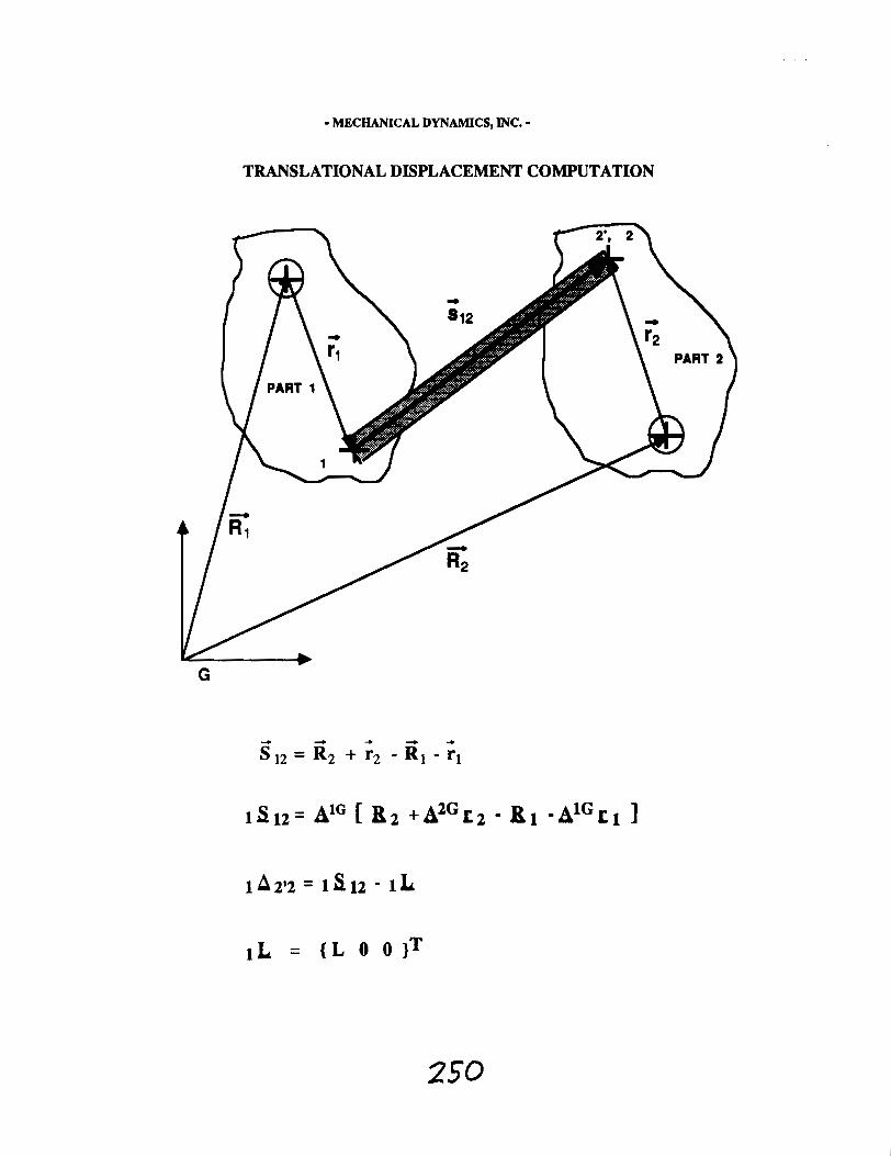
- MECHANICAL DYNAMICS, MC. -
TRANSLATIONAL DISPLACEMENT COMPUTATION

- MECHANICAL DYNAMICS, INC. -
ANGULAR DISPLACEMENT COMPUTATION
SPACE 1-2-3 ANGLES ARE USED FOR MEASURING ANGLES
fi2 A SIN-^(-^^,)
IF fi2 # n / 2 THEN
fi3 = ARCTAN2 ( a ,, + a 13, a 13 - a 22 ) - 0 1
ELSE IF fi2 = n I 2 THEN

- MECHANICAL DYNAMICS, INC. -
VELOCITY COMPUTATION

- MECHANICAL DYNAMICS, JNC. -
FORCE COMPUTATION
& IS THE STANDARD MATRIX FOUND IN ANY STRUCTURAL ANALYSIS TEXT
F O R O E s-
SINCE THE BEAM IS MASSLESS, APPLYING LAWS OF EQUILIBRIUM :

- MECHANICAL DYNAMICS, INC. -
c
DIRECTLY RELATED TO DEGREE OF DISCRETIZATION
METHOD DOES NOT YIELD WRONG ANSWERS
DEGREE OF DISCRETIZATION DEPENDENT ON FREQUENCY
CONTENT DESIRED. ADAMS/MODAL WILL COMPUTE
EIGENVALUES AND EIGENVECTORS FOR ANY ADAMS MODEL.
CAN ANIMATE LINEAR MODEL USING SELECTED SET OF MODE
SHAPES AND FREQUENCIES.

R.R.Ryan (313) 936-2922 University of Michigan
FLEXIBLE BODY DYNAMICS Benchmark Problem #1: Uniform Cantilever Beam Spin-up
T h e inset of Fig. 1 shows a uniform, homogeneous, cantilever beam supported by a circular hub of radius r. At time t = 0, t h e system is a t rest in a Newtonian reference frame and the beam is undeformed. Subsequent t o this initial time, t h e hub is made t o rotate about a vertical axis X - X , passing through the center of the hub, in such a way t h a t R , the angular speed of the hub, is given by
~ ( t ) = (215) [1 - (7.5/z)ein(r1/7.5)] rad/rc 0 < t < 1 5 sec 6 radlsec t > 15 eec
which represents a smooth transition from zero hub motion t o a constant angular speed of 6 rad/sec. T h e beam has a length L, Young's modulus E, shear modulus G, mass per unit length p, and a circular cross- section of area A and area moment of inertia I.
T h e solid line in the figure below shows the time history of the displacement of the beam tip. in the plane of rotation, relative t o a line fixed in the hub and originally parallel t o the centroidal axis of the beam. This result was obtained using the theory and algorithm presented in Refs.[]] and [2] with three assumed modes and the following parameter values
All external forces were neglected and the assumed modal functions were chosen t o be equal t o the first three eigenfunctions of a n identical uniform cantilever beam with its root fixed in a Piewtonian reference frame. T h e numerical integration was carried out using a 41h - Sh order, variable step-size, Runge-Kutta-hlerson method with a print s tep and initial time s tep of .03 seconds and an error tolerance of 1 x T h e dashed line result was produced with an algorithm based on the assumed-mode formulation utilized in most flexible multibody programs. This result was verified by Fidelis Eke [(818) 354-2916] a t J e t Propulsion Labs using DISCOS.
t 001 J,
4
4s-. W 0 10.0
-0.1) -. Tim e (3 ec .]
-0.s .. Tip X
Disp. -02.. Inplane
(m) 4 . 4 s - . l i p displacement
--- - WNVE~ONAL 4 b S ..
-0.a 1 \ \
-0.11;- \ X L \
FQ. 1 Spin-up of Homogeneous Uniform Cantilever Beam
[l] Ryan, R.R. , "Flexibility Modeling Methods in hlultibody Dynamics," Ph.D. dissertation, Stanford University, Available frcm University hlicrofilms, Ann Arbor, hl ich~gan, 1986.
[2] Kane. T.R., Ryan. R.R. , and Banerjee. A . K . , "Dynamics of a Cantilever Beam Attached t o a hlovinf; Base,'' Journal of Guidance. Conirul, and Dynamzcs, Vol.10, No.2, Rlarch-April. 1987.


UNIFORM BEAM SPIN - UP PROBLEM : ADAMS APPROACH
BEAM TIP DEFLECTION Vs. TIME
- tl3

- MECHANICAL DYNAMICS, INC. -
THIS METHOD IS USABLE FOR SMALL TO MEDIUM SIZE PROBLEMS
( MEDIUM = 300 RIGID AND FLEXIBLE DOF )
FOR LARGER PROBLEMS IT MAY PROVE TO BE MORE CPU INTENSIVE
THAN DESIRABLE.
THE CPU TIME TAKEN FOR A SIMULATION IS LINEARLY
PROPORTIONAL TO THE NUMBER OF FLEXIBLE BEAMS IN
THE SYSTEM


- MECHANICAL DYNAMICS, INC. -
EASE OF USE
THE RESULTING PROGRAM IS EXTREMELY EASY TO USE.
USERS DO NOT NEED STRONG FEA BACKGROUND TO CREATE
MODELS OF STRUCTURES
RECOGNITION AND SELECTION OF PROPER MODES IN AN ART.
THE RESULTS ARE ONLY AS GOOD AS THE SELECTED MODES.
DIFFICULTY ALLEVIATED IN THIS APPROACH.

- MECHANICAL DYNAMICS, INC. -
NODES
LOCATION OF NODES 2 , 3 , 4 WRT. TO A KNOWN REFERENCE FRAME
MASS AND INERTIA PROPERTIES FOR EACH NODE OBTAINED FROM MASS MATRIX.
LOCATION AND ORIENTATION OF COORDINATE SYSTEMS
2 ON PART 2 2' ON PART 1
3 ON PART 3 3' ON PART 1
4 ON PART 4 4' ON PART 1
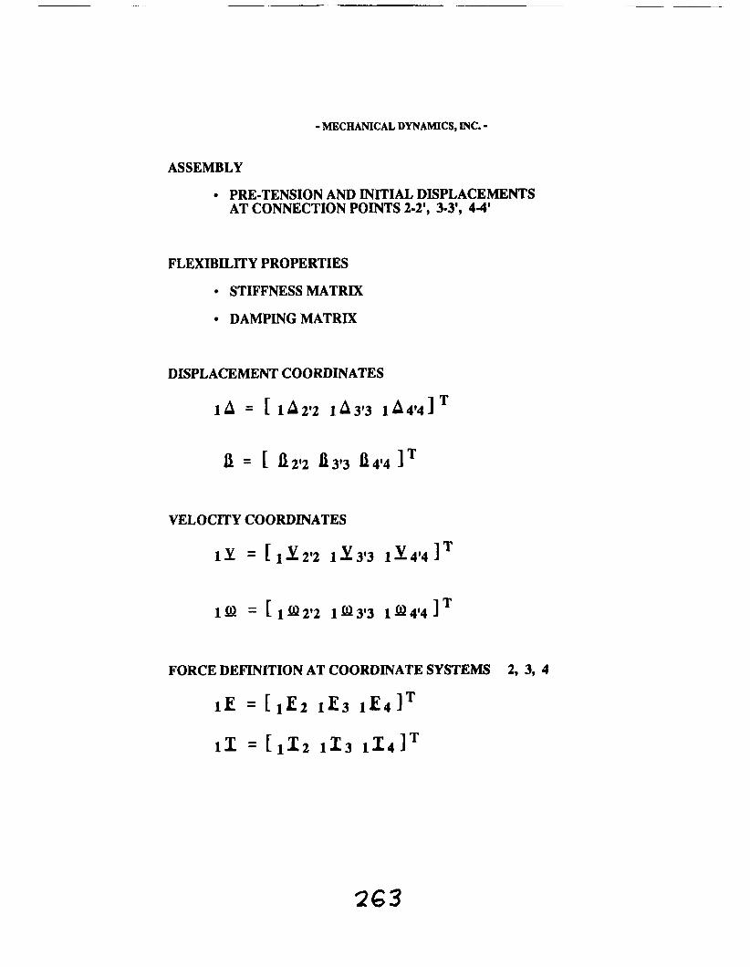
- MECHANICAL DYNAMICS, INC. -
ASSEMBLY
PRE-TENSION AND INITIAL DISPLACEMENTS AT CONNECTION POINTS 2-2', 3-3', 4-4'
FLEXIBILITY PROPERTIES
STIFFNESS MATRIX
DAMPING MATRIX
DISPLACEMENT COORDINATES
1 4 = [ 1 A t f 2 1 A 3 3 1 ~ 4 1 4 1
VELOCITY COORDINATES
1 Y = r 1 Y 2'2 1 Y 3'3 I Y 4l4 I T
FORCE DEFINITION AT COORDINATE SYSTEMS 2, 3, 4

- MECHANICAL DYNAMICS, INC. -
FORCE COMPUTATION AT COORDINATE SYSTEMS 2,3,4
FORCE AT COORDINATE SYSTEM 1

A Comparison of Software for the Modeling and
Control of Flexible Systems
Lawrence W. Taylor, Jr. NASA Langley Research Center
Computational Aspects Workshop July 12- 14, 1988 Williamsburg, VA

Memorandum
To: W horn it may concern
From: 16 1 /Chief Scientist, GCD
Subject: Development of Software for the Control of Flexible Systems
I-pwpae a cooperative effort among specialists who use or develop software for simulating and analyzing the control of flexible, aerospace systems. A comparison of existing software for modeling control systems and flexible structures, applied to several example problems would be quite valuable. The comparison would indicate computational efficiency and capabilities with respect to handling nonlinearities and graphical output. , ,. , 4 e , - , + / e ,
\ ,$. " 4 < ,- + ' J I I
Because of the diversity of applications of such software:@belim that the proposed cooperative effort can transcend projects involving specific applications. Comparisons of software capability and efficiency can be made and gaps can be identified. In this way the results of the cooperative effort can provide guidance for individual projects.
Ewdewdafe ~evera l charts which outline the objectives and approach of the proposed'cooperative effort. I--woufd appreciate your suggestions - a&-~p~essions of interest in -this matter.
; j L ., i yulu7& Lawrence W. Taylor, Jr. Mail Stop 161 NASA Langley Research Center Hampton, V A 23665 (8041-865-459 1
KEGliDkiU@ F&E BUNK NOT FILMED
26 7
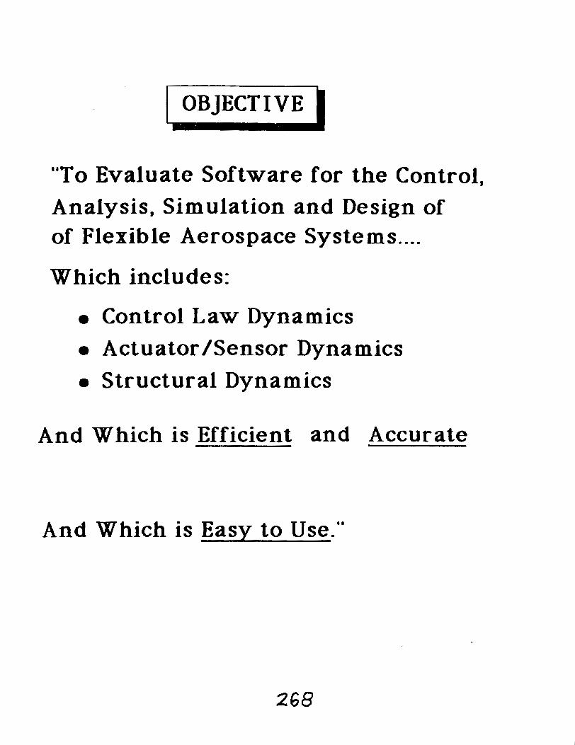
( OBJECTIVE I
"To Evaluate Software for the Control, Analysis, Simulation and Design of of Flexible Aerospace Systems... .
Which includes:
Control Law Dynamics Actuator/Sensor Dynamics Structural Dynamics
And Which i s Efficient and Accurate
And Which is Easy to Use."

I APPROACH )
(Organize Users and
1 --- ---_ ---- --- */- --
( ~ e l e c t Example Problems
\ < \- Identify Gaps in Capability -0 , ---- /--/ ---- ---_ _--- ----

I Example Problems
Unif or m Beam - Pinned -Pinned
I SCOLE (L. T a y l o r - L a R C )
SAFE (70 x D e p l o y m e n t ) ( L . T a y l o r - L a R c )
Pinhole O c c u l t e r ( H e n r y W a i t e s - M S F C )
M a n n e d Space Station a. Reboost b. Solar Dynamic Pointing c . MRMS Operation d . Docking
O t h e r s ?
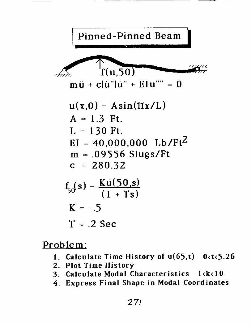
Pinned-Pinned Beam I
u(x.0) = Asin(TIx/L) A = 1.3 Ft. L = 130 Ft. E I = 40,000,000 ~ b / ~ t ~ m = -09556 Slugs/Ft c = 280.32
5Js) = K u ( ~ , s ) ( 1 + Ts)
T = -2 Sec
Problem: 1 . Calculate Time History of u(65,t) 0 m 5 . 2 6 2. Plot Time History 3. Calculate Modal Characteristics 1 <k< I0 4. Express Final Shape in Modal Coordinates

I CSI Simulation Software 1
NASTRAN
DISCOS
TREETOPS(CONT0PS)
EAL ORACLS
LATDYN EISPAC
DADS LINPAC
Multi-MACS Matrix,
CTRL-C
SYSPAC

1 Information Sheet b NAME of SOFTWARE: DISCOS
RESPONSIBLE PERSON: Harry F r i s c h NASA Goddard Space Center Bldg. 1 I , Rm. S221A Greenbelt, MD 2077 1
CAPABILITIES: 1. Nonlinear Kinematics? yes d NO
2. Finite Element Modeling? yes E( NO
3. All Rotational and Translational D.O.F.? Y e s d No 4. Linked to Distributed Parmeters? Yes0 No0 5- Large Amplitudes? yes d NO q 6- Nonlinear Damping? yes 0 NO e( 7. Control Law D l namics? yes • NO d 8. Sensors and Actuator Dynamics? yes NO d 9. Nonlinear Joints? yes NO d
1 0. Distributed Parameter System? yes 0 NO td 1 1. Optimal Control Synthesis? yes 0 NO d 12. Sensitivity Functions for P.E. & Design? Y e s 0 No d
DOCUMENTATION: Complete-
SIZE: SOOK
LANGUAGE: Fortran 77 +
INTERACTIVE: NO.
GRAPHICS: plots
Free, Nonproprietary AVAILABILITY:

( Information Sheet 1 NAME of SOFTWARE: LATDYN
RESPONSIBLE PERSON: Jerry Housner Mail Stop - 230 NASA Langley Research Center Hampton. VA 23665
CAPABILITIES: 1 . Nonlinear Kinematics? yes d NO 2-D-0-F- 2. Finite Element Modeling? yes $ NO 2-D-0-F- 3. All Rotational and Translational DO.F.? Yes d No 2-D-o-F- 4. Linked to Distributed Parmeters? yes d NO 2-D-0-F- 5- Large Amplitudes? yes d NO 2-D-0-F- 6. Nonlinear Damping? yes d NO 0 Add Code 7. Control Law Dynamics? yes d NO 0 Add Code 63. Sensors and Actuator Dynamics? yes d NO Add Code 9. Nonlinear Joints? yes Bf NO Add Code
10. Distributed Parameter System? yes d NO 2-D-0-F- 1 1 . Optimal Control Synthesis? yes o NO d 1 2. Sensitivity Functions for P.E. & Design? Yes NO d
DO CUMENTA TION : 2-D.0-F- Written, 3-D.O.F. Under Development
SIZE: ~ O O K
LANGUAGE: Fortran 77
INTERACTIVE: Yes
GRAPH1 CS: Time Histories. Line Drawing, PSD. Movies
AVAILABILITY: Free, Nonproprietary

/ Information Sheet 1 NAME: Mult ibody A n a l y s i s ( Control S y n t h e s i s (MACS)
RESPONSIBLE PERSON: Lawrence W. Taylor NASA Langley Research Center Hampton, VA 23665 (804) -865-459 1
CAPABILITIES; 1 . Nonlinear Kinematics? yes d NO
2. Finite Element Modeling? yes d NO
3. All Rotational and Translational D.O.F.? Y e s d No 4. Linked to Distributed Parmeters? yes PI NO
5. Large Amplitudes? yes d NO
6. Nonlinear Damping? yes NO d Not Y e t 7. Control Law Dynamics? yes d NO
8. Sensors and Actuator Dynamics? yes d NO
9- Nonlinear Joints? yes NO d Not Yet 1 0. Distributed Parameter System? Y e s NO d 1 1 . Optimal Control Synthesis? yes NO d
DOCUMENTATION: Incomplete
SIZE: 25K Core Memory
LANGUAGE: FORTRAN 77
INTERACTIVE: No
GRAPHICS: None
AVAILABILITY: No Charge

Infor mation Sheet
NAME of SOFTWARE: TREETOPS (CONTOPS)
RESPONSIBLE PERSON: Ramen Singh Dynacs Engineering Company 2280 U.S. 19 No.. Su i t e 1 1 1 Clearwater. FL 34623
CAPABILITIES: 1 . Nonlinear Kinematics? 2. Finite Element Modeling? 3. All Rotational and Translational D.O.F.? 4. Linked to Distributed Parmeters? 5. Large Amplitudes? 6. Nonlinear Damping? 7. Control Law Dynamics? 8. Sensors and Actuator Dynamics? 9. Nonlinear Joints?
1 0 . Distributed Parameter System? 1 1. Optimal Control Synthesis? 1 2. Sensitivity Functions for P.E. 6 Design?
DOCUMENTATION:
SIZE:
Y e s d NO
Yes d NO
Y e s d NO II Y e s PJ NO
yes d NO - Yes PJ NO
Y e s d NO
Yes d NO o Y e s PI NO
Y e s d NO
Y e s NO d Y e s NO d
Complete. Course Available.
LANGUAGE: Fortran 77 +
INTERACTIVE: Yes. Sun, MicroVAX, Masscomp
GRAPHICS: Plots, Windows, Movies
AVAILABILITY: Free, Nonpropriety

I Information Sheet
NAME of SOFTWARE:
RESPONSIBLE PERSON:
CAPABILITIES: 1. Nonlinear Kinematics? 2. Finite Element Modeling? 3. All Rotational and Translational D.O.F.? 4. Linked to Distributed Parmeters? 5. Large Amplitudes? 6. Nonlinear Damping? 7. Control Law Dynamics? 8. Sensors and Actuator Dynamics? 9. Nonlinear Joints?
1 0. Distributed Parameter System? 1 1. Optimal Control Synthesis? 1 2. Sensitivity Functions for P.E. 8 Design?
Y e s O No0 YesU No0 Y e s q No q Y e s O No0 Yes q No Yes q No q YesU No0 YesO No0 Y e s q No q Y e s q No q Y e s q No Yes q No U
DOCUMENTATION:
SIZE:
LANGUAGE:
INTERACTIVE:
GRAPHICS:
AVAILABILITY:

Solution Characteristics
Time Required - CPU Sec.
Accuracy a. Modal Characteristics b . Time Histories (PSD)
0 Memory Required
Input
Output

PANEL DISCUSSION
1. Should We Compare Software for
ControlIModeling?
2. Should W e Establish Example Problems?
3. Should This Workshop be Repeated?
Changed? ..................... .................... Merged?.

SESSION III - COMPUTATIONS EFFICIENCY AND CAPABILITY
PRECWlffi PAGE BLANK NOT FLMED
A FINITE EISlUENT APPROACH FOR LARGE MOTION DYNAMIC ANALYSIS OF MULTIBODY STRUCTURES IN SPACE
Che-We1 Chang The COMTEK Company
Crafton. Virginia
ABSTRACT
A three-dimensional finite element formulatlon for modeling the transient dynamics of constrained multlbody space structures with truss-llke codlguratlons Is presented. <:onvected coordinate systems are used to define rigid-body motion of Indivldual clrrnents In the system. These systems are located at one end of each element and are orlcnted such that one axis passes through the other end of the element. Deformation of c-ach element. relative to 11s convected coordlnate system, is defined by cublc flexural shape functions as used In h l t e element methods of structural analysis. The forn~ulatlon I s oriented toward joint dominated structures and places the generallzed coordinates at the jolnt. A transformation matrix is derived to integrate jolnt degree- of-freedom into the equatlons of motion of the element. Based on the derwation. a general-purpose code LATDYN (Large Angle Translent DYNarnics) has been developed . Two examples are presented to Illustrate the application of the code. For the spin-up of ;I flexlble beam. results are compared with exfstlng solutions available in the llterature. For I he deployment of one bay of a deployable space truss (the "Mlnlmast'). results are verirled by the geometric knowledge of the system and converged solullon of a successively reflned model.
PRECFalFjG PAGE Di&NX N;ii FLLMED
283

brge &gle xturmiant P]Muicm
(Finite-Element-Based)
A NASA Facility for
in
Application. and Analy8im Techniques
for Space Structure Dynamic8
Qraa.nt.4 by
Che-Wei Chang
OOCItlt
284

* Motivation * Capability * Theory * Modelling * Present LATDYN
(verifications)
* Future LATDYN
* Conclusions

* Three-Dimensional * Deformable Bodies * Multi-Connection Joints
* Large Angular Motion * Variable Constraints
* Impacts & Joint-Lock
* Experimental Data * User's Control Strategy

1. Corotational Axer (convected system)
2. F-E Connectivity through
Joint Kinematics
3. Numerical Integrations

.DEFORMED FINITE ELEMENT AND ELEMENT COORDINATE SYSTEMS

Deformation : u

Internal Force
virtual work done by internal farce

Total displacement
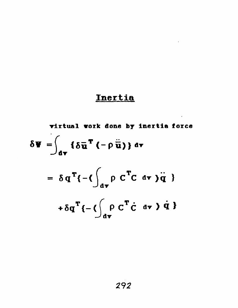
Inertia
virtual rark done br inertia force

TYPICAL lNT ERCONNECTION OF TWO JOINT BODIES
T HROUOH FLEXlBLE BEAM
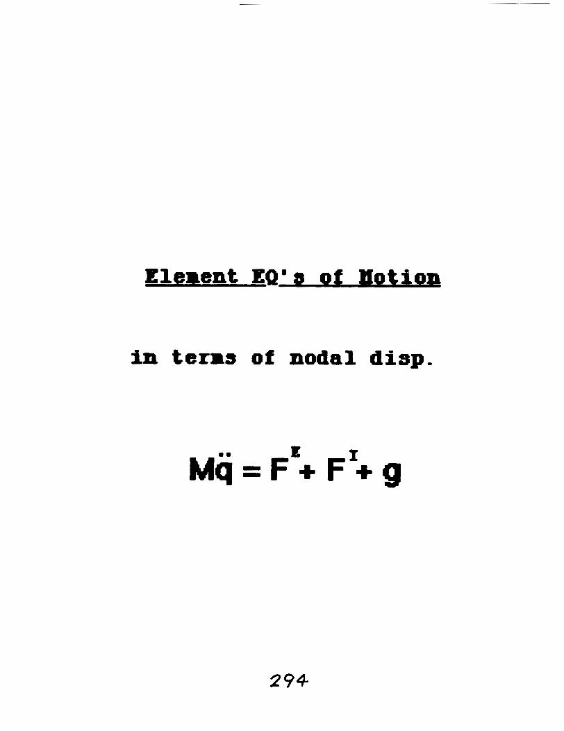
Element EQB s of Hotion
in terms of nodal diap.


Joint Kinematics

oint Body .

generalized coard.

at each joint body:
3 translational disp.
3 orientational disp.
+ No. of relative(joint)
d-0-f ' 8

in terms of joint body
apd joint dof ' s

Equations of Motion and Their Numerical Integration
At nth time step,
Mnan + f I' + !ln = F~
Newmark-Beta Integrator at kth iteration:
h -1
2 ~ n - 1 it; :Update Acceleration: up = a;-, + [M;'-, + -GE-, + ph 2
R: = iterative residual = Fn - f,ll - M,"_,a:-,
V; - - vn-1 + (5) (an-I + a;) :Update Velocities

* Bow doe. user work w i t h
WTDYN 3
* How doe8 program modal
a syetem ?

' d v r i c \
results , ---_
~ - - p a Z p r o ~ s s s o f - - - - - -- ---__ _--- ---&' -- I
( graphics )
___----- ------_____ ..- -- --
(..- -_ preproce3sor -. -..I -.. -- ---_ --- __---- -- ,---
_--- -- ---_ .#@--- ---.
<._ --- ----- ----- user > 305
-
1 1 v 7 d
model user's \
data - subroutines \ 1
11 _---- ---_ 11 ----__ -- LATDmr _ --- _.I. --.) ----- - - _---
B

1. Numerical Control
2 . Flexible Bodies
* material properties * element properties * grid points
3. Rigid Connections
* body geometry & mass
* joint connection.
4. Forcing Elements
* Forcing function. * spring-damper-actuators
5 . I n i t i a l Conditions
6. programmable language
307 ORlGtNAL PAGE BLACK AND WHITE PHOTCX3RAW

z= E m "I-
. . $ 's Y
nJ - : X L
0
"J 2
m * OJ - tz > u 0 0 5 v o c m
DL g-I! 0 YLW ~n a~ s
00 L <a I lA
.. = 0 .
W Z h COW" s++ 0 .%3+ CT
ORlGlNAt PAGE: B~~ AND 'WB TE. P I . ~ k ~ ~ ~ p ~ l
k- a 0
MECEDlNG PAGE BLANK NOT FILMED 309 a 3 0 f N W D o I I I I l y ~

Conventional
P-E Hodel of c o m e r body -
grid (6-dof's)

F-E Hodel of comer bodx grid (6-dof ' s)
0 hinge ( I - d o t )

3-D LATDYN Model of Mini-Mast
Locking Joint
Note: closed loop
Target is that user will not have to specify how rigid members are formulated.
Program will determine most efficient arrange- ment, and will cut closed loops and implement constraints automatically.
312

* three-dimensional * Euler-Bernoulli beam
elements
* hinge connections
* ~ewmark-P explicit h
implicit methods
* constraints & joints
* external forcing function & spring-damper-actuator

COMPARISON OF RESULTS FOR FLEXIBLE BEAM SPIN-UP ON A PLANE
O.02r 1 I 1 1 I I 1 1 1 +
b
0.m 3
-0.02 - u
...
-0.04 - - - DADS PROGRAM
-0.w- - .-
-0.00' 1 I I I I I 1 1 I 1 1 1 I I I I 1 I 1
0. 1. 2. 3. 4. 6. 6. 7. 8. a. 10. A
Timelfundamental Period

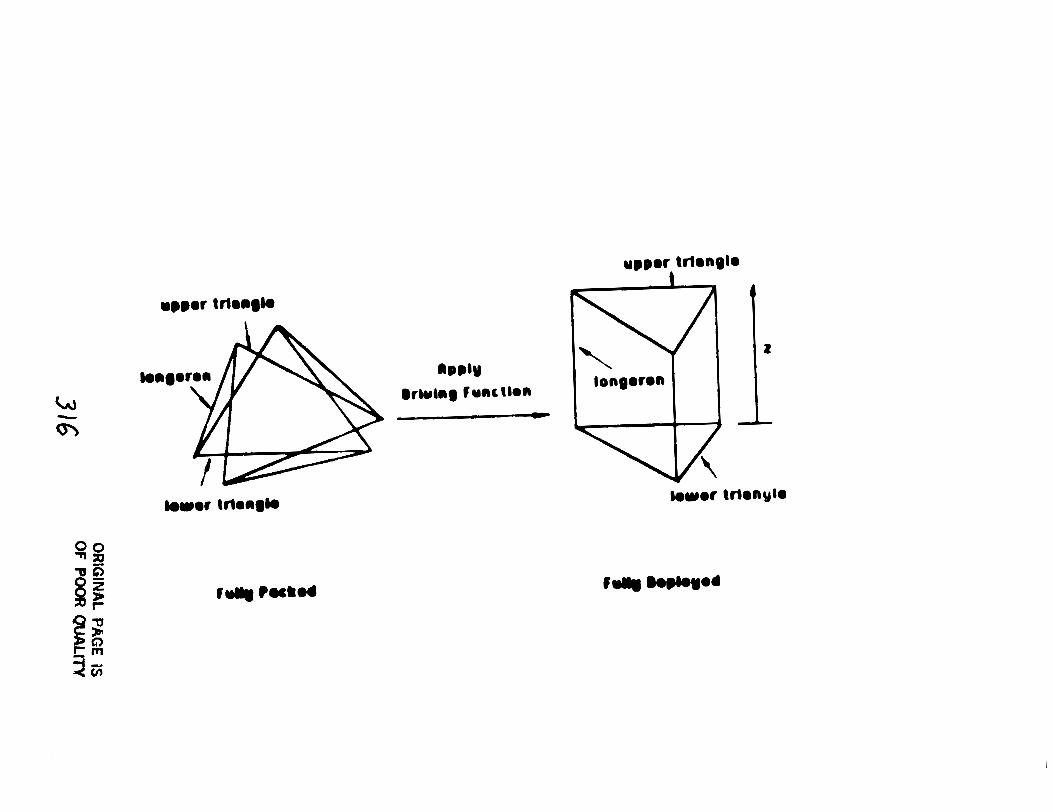
OR
IGIN
AL P
A6E
1s O
F POO
R QU
ALtTy

0.5
0.0
-0.5
- 1 .Od
- Uppor Joint
- DESIRED - ------ UNCONS' - - L
L
C
- - D
L
C
m
- C
D
C
- I L I I I I I I I I I I I 1 I I 1 I 1 I I 1 I I
-1.0 -0.5 0.0 0.5 1 .O
X COORDINATE

F O U R E ------ TWO EL --- ONE EL - A S T R O
LONGERON ANGLE

AT UPPER JOINT
LONGERON ANGLE

* various elements * various joint connections * various integrations
(parallel version)
* control and structure interactions

* A finite-element-based
research code is developed.
* It provides a modelling, calculrtion, and analysis
tool for researcher C E n g t .
* T o analyze complex apace
structures and/or mechanisms.
* In the simulation of
C o n t t o l dasign as well as
structural dynamics.

ENHANCED ELEMENT-SPECIFIC MODAL FORMUIATIONS FOR FLEXIELE MULTIBODY DYNAMIC8
Robert R Ryan University of Michigan Ann Arbor. Michigan
ABSTRACT
The accuracy of current flexible multibody formalisms based on assumed modes is examined In the context of standard spacecrait motlons involving structural components undergoing both slow and fast overall translational and rotational motions as well as small deformations. Limitations of current techniques in treat- (1) element-speclfic coupling behavior of large motion and small deformation, and (2) motion-induced structural stlITness variations. are noted.
The roles of nonlinear and linear elastic structural theories in accurately predicting lransient large-displacement dynamic behavior of flexible multlbody systems are examined In detail. Coupling effects between deformation and overall motion are carefully scrutinized in the context of assumed-mode discretization techniques. Consistently linearized beam. plate. and shell formulations involving in-plane stretch variables are proposed and shown to yield very accurate simulation results and exlremely fast modal convergence for most motions involving small strains. In some particular cases. however. In whic~membrane'stiITness dominates bending stiffness. a nonlinear strain formulation is requhed in order to capture proper coupling between tieformalion and overall motion. Unfortunately, with standard component modes. algorithmic formalisms involving nonlinear strain-displacement expressions show very slow modal convergence. A procedure involving use of constraint modes is proposed to alleviate thls problem.
PREC6jDING PAGE B U N K NOT FlLMED
t &TENT-# BUM


W I N A L PAGE IS OP KW)R QUALITY

I. Limitations of Existing Flexible Multibody
Formalisms
Examples a Verification
11. Linear and Nonlinear Element-Specific Formulations
Consistently-Linearized Beam, Plate, Shell Multibody Models
a Second-Order Beam, Plate Models
111. Simulation Results
a MembraneIBending Problems
Convergence

Current Flexible Multibody Formalisms - Modal Approach "Limit at ions"
Do Not Account For Large-Displacement Element-S pecific Behavior
Inadequate Account of Motion-Induced Stiffness Variations
I Finite Element I Component Model I
* -
Structural Model s \ BEAMS, PLATES, SHELLS,
AXISYMMETRIC SOLIDS, 3-D SOLIDS, PLANE STRESS, PLANE STRAIN, etc.
I Flexible Multibody 1
3-D CONTINUA u
Eigensolut ion Modal Integ
Processor \ r ( (.onlinear )I
PRECEDING PAGE B U N K NOT FlLMED
u s r 3 3 0 m w w

Slow Re~ositional Maneuver of Channel Beam
Repositional, Maneuver Angle
@(t)
15.0 30.0
Time (sec)

n - - Awn& 2 w V 2s so
Multibody Formalisms -----
I I I I I I I
Time (sec) 335

~ [ A / I h//7# oFFSf7 7 i P MASS
CTt4 1
I
P 1
'Sp.
71 ~e
P 1 F
337 PRECEDlNG PAGE BLANK NOT FWED
an TP
BSP
1
h e n
u3'3 .#,EN-

nstant Speed Spin - Buckling Analysis. Conventional Vs. Enhanced Modal Theory
Time (seconds)
- BEAM-SPECIFIC FORMULATION L/R = 0.5
Enhanced Modal Formulation[l21 / Ryan - 1985. - Agrees with Kammer, schlack[171 - 1984.
-
-
-
-
-
-
- Agrea with Peters, ~ o d ~ e s [ l ~ ] - 1980. - Out-of-Plane Buckling Eqs. eame as
White, Kvaternik. K u a [19] - 1979
u ~ ~ ~ ~ ~ ~ ~ ~ ~ ~ ~ ~ n MULTIBODY FORMULATION[^-111 Generic-Body Assumed Mode Formulation


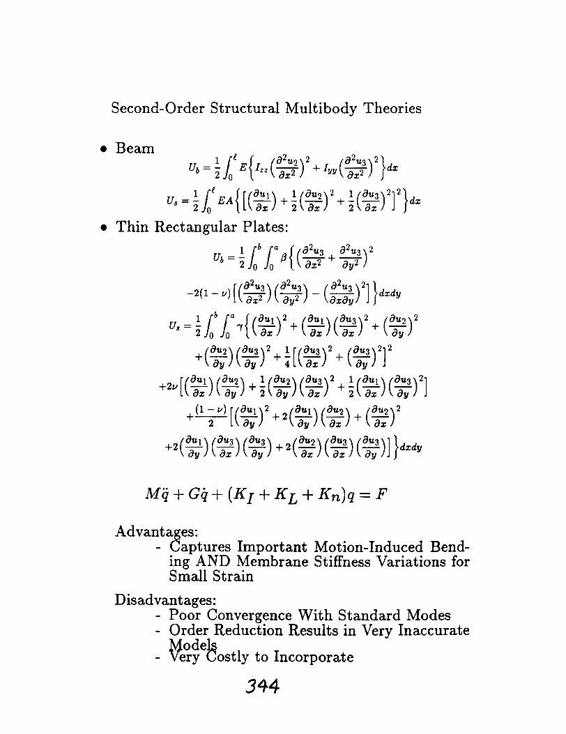
Second-Order Structural Multibody Theories
Beam
Thin Rectangular Plates:
Advant?!ztures Important Motion-Induced Bend- ing AND Membrane Stiffness Variations for Small Strain
Disadvantages: - Poor Convergence With Standard Modes - Order Reduction Results in Very Inaccurate
ode - Very kostly to Incorporate

Transverse Tip
Displacement (meters)
SMOOTH SPIN-UP MOTION (0 - 6 rad/sec in 15 seconds)
SMOOTH SPIN-UP MOTION (0 - 6 revlrnin in 30 seconds)
Midpoint Transverse
Displacement (inches)
-I - - -5 .E- l
El 28 Time (seconds) 4a 60
I I I I I I I I I I I I

SIMPLY SUPPORTED RECTANGULAR PLATE SPIN-UP MOTION Assumed Mode Approach with Nonlinear Strain Expression
Tramverse Deflection of Center of Plate - Smooth Spin-up From 0 - 6 rad/sec in 15 seconds
I -- -
1
sec
m
a
m
- -
m
0 10 20 3
Time
Raulta obtained with 3 Assumed Stretch Modes and 3 Assumed Bending Modes
I I I I I I I I 1

Static Analvsis of a Sauare Plate with
Uniform Pressure Distribution Considering v Membrane Stiffneu
Uniform Pressure p
Simply Supported
Maximum inertia force per area in the middle of the plate during the spin-up motion is used as uniform pressure distribution.
Fig. 19 - Static Deflections under High Pred8ure Loads
347
Static
YS 0.18"
IC 0.32"
Dynamic
Present
0.21"
0.37"
Conventional
2.1"
Divergence #


EFFICIENCY AND CAPABILITIES OF HULTI-BODY SIHULATIONS
R.J. VanderVoort DYNACS Engineering Co., Inc.
Clearwater, F1
ABSTRACT
Simulation efficiency and capability go hand in hand. The more capability you have the lower the efficiency will be. -s
fficiency and --th capabilities. The lesson -bout generic simulation is: Don't rule out any ~apabilities at the beginning but keep each one on a switch so it can be 4ypassed when warranted by a specific application,
--.
Efficiency means different things to different people. For the person running simulations interactively on a terminal quick turn around time is efficiency. For the person making 10,000 Honte-Carlo runs low cost is ef- ficiency. For the person running real time simulations minimum CPU time is efficiency.
Three aspects of a simulation should be considered when dealing with efficiency; hardware, software and modeling.
Eardwarg A fast processor will reduce CPU time for a given simulation but this doesn ' t necessarily equate to improved efficiency . For example, the Monte-Carlo simulation may take 10 minutes on a super computer and 2 weeks on a PC but if time is free on the PC then that may be an efficient solu- tion. We will not discuss hardware related issues except for two points. 1 .) Past hardware is of primary importance to the real time simulation because it means higher fidelity models can be incorporated 2.) Vector processors and parallel processors should use custom algorithms that take full ad- vantage of the special machine architecture.
Software A fast algorithm will also reduce CPU time but again this doesn't necessarily equate to improved efficiency. For example, i t is generally accepted that an ad-hoc simulation is much faster than a generic simulation. The cost of developing and testing the ad-hoc simulation may exceed the run time saving thereby reducing overall efficiency.

Recent work in the area of symbolic programming has shown that sig- nificant savings can be achieved by symbolicaly forming the equation of motion and numerically solving them. Other algorithms have been proposed that promise similar savings, There is one point that software developers should keep in mind. With generic simulations the user muat have complete flexibility in retaining or deleting different parts of his model. This is because generic simulations are often used for model development and valida- tion. In that environment an analyst vill add or delete certain features to determine the effect on performance and vhether or not the feature should be retained in the model.
Hore on this subject in section 2.
Hodelin& This is the domain of the simulation user and the area in which many improvements in efficiency can be made. For exaaple, deleting a high order mode in a flexible body model has a compound effect. It reduces the model complexity and at the same time allovs a bigger integration step size both of which reduce run time. Often times the reduced fidelity is justified by the savings in run time.
The point to be d d e is that the analyst la the end authority on the Wcorrectu model for a given application. The more flexibility he has in changing his model the easier it is for him to select the best model for the job.
2. CAPABILITIES
Capability in our context is synonymous vith f l e x i b i i ~ and not vith complexity. A simulation may be very detailed and complex but if it can't be changed then it's only useful in a narrow range of applications and has limited capability.
In our experience with TRBBTOPS and DCAP we have found that it is much easier to generate a model and obtain a reeponse than it is to predict the correct response. In other words, when we donp t get the expected response the simulation is usually correct and our expectation is wrong. This is not entirely unexpected because it is very difficult, even for an expert, to solve the equations of anything but the simplest dynamical systems. The solution to this dilefna~a is flexibility. Start vith simple models that have known analytic solutions, Then add complexity one step at a time while gaining confidence in your model and insii!ht into the behavior of your sys tea,

For multibody systems with flexible bodies the same arguments apply but the complexity of the model increases more rapidly than for rigid bodies. The person doing software development makes assumptions that simplify the resulting equations of motion. If this is done carelessly then terms are dropped that may prove essential in specific applications. On the other hand, if simplifications are not made then the computation burden becomes too great.
The lesson we learned is that you must retain as many terms as possible in the kinematics but they must have associated switches so you can easily add or delete them from a specific application. This is done for two reasons. 1 .) to give you insight into the effect of various model elements on system response and 2.) to allow the selection of the most efficient model for a given application.

f i SIMULATION EFFICIENCY
HARDWARE n BYPASS TERMS BYPASS TERMS MULTI-RATE ALGORITHMS INTEGRATION TYPE & STEP SIZE SYMBOLIC PROGRAMMING REDUCED ORDER ADHOC SIMULATION
4

SPEED-UP OPTIONS
COORDINATE TRANSFORMATIONS
/ PERFORM ALL I COMPUTATIONS
COMPUTE ONLY ON
FIRST PASS OF A-K
INTEGRATION COMPUTE ONLY ON FIRST PASS OF NTH
A-K STEP BYPASS
COMPUTATIONS
MASS MATRIX FORMULATION
(MI
NON-LINEAR I CONSTRAINT I TERMS
( ~ 3 x 1 - w ) I FORMULATION I

TREETOPS SOFTWARE IMPROVEMENTS
QBG EQUATION FORMULATION
EQUATION SOLUTION
PROCESSING HARDWARE
CURRENT STATUS tt -h FIRST STEP
SECOND STEP
NUMERIC v
SYMBOLIC
SYMBOLIC
NUMERIC
NUMERIC
NUMERIC
SERIAL
SERIAL v
PARALLEL

SIMULATION CAPABILITY-MENUS
E%G BODIES SENSORS ACTUATORS CONSTRAINTS DEVICES CONTROLLERS
1. RIGID 1. RATE GYRO 2. FLEXIBLE 2. RESOLVER
3. ANGULAR ACCELEROMETER
4. VELOCITY bl 5. POSITION
6. ACCELEROMETER 7. TACHOMETER
8. INTEGRATING RATE GYRO
9. SUN SENSOR 10. STAR SENSOR 11. IMU 12. POSITION VECTOR 13. VELOCITY VECTOR
1. REACTION JET 1. CLOSED LOOP 1. SPRINGS 1. CONTINUOUS 2. HYDRAULIC 2. VELOCITY-TIME 2. DAMPERS 2. DISCRETE
CYLINDER 3. VELOCITY 3. COULOMB 3. BLOCK DIAGRAM 3. REACTION -UIRECTION DAWER (FREQUENCY
WHEEL 4. RATE-TIME 4. QUADRATIC DOMAIN) 4. TORQUE 5. RATE-DIRECTION SPRING/DAMPER 4. MATRIX
MOTOR 6. CUT JPINT 5. SOLID DAMPER (STATE SPACa 5. MOMENT 6. HARDSTOP 5. USER 6. BRAKE 7. CONTACT 7. LOCK SPRINGS
8. SINGLE 6IMBAL CM6
9. DOUBLE 6IMBAL CM6
10. MAGNETIC
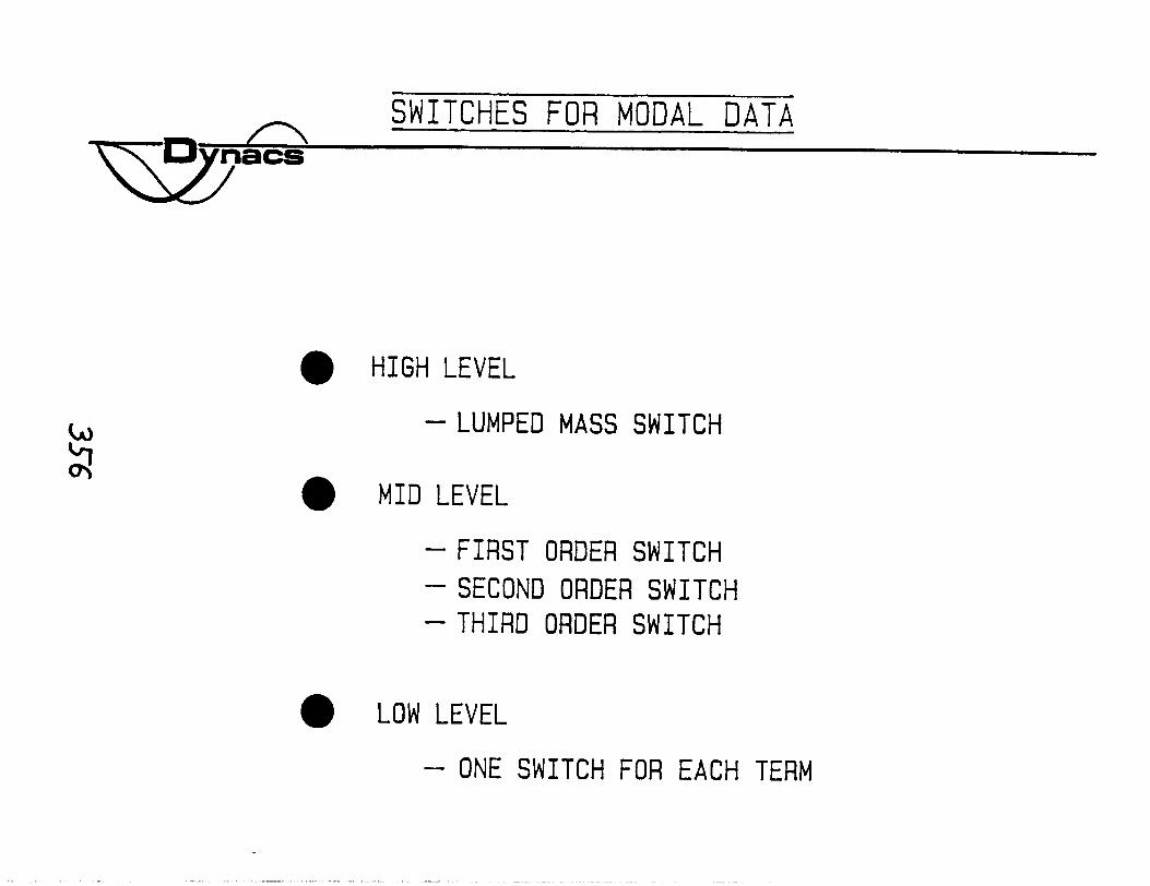
=I--U
+
HI--
HZ
H

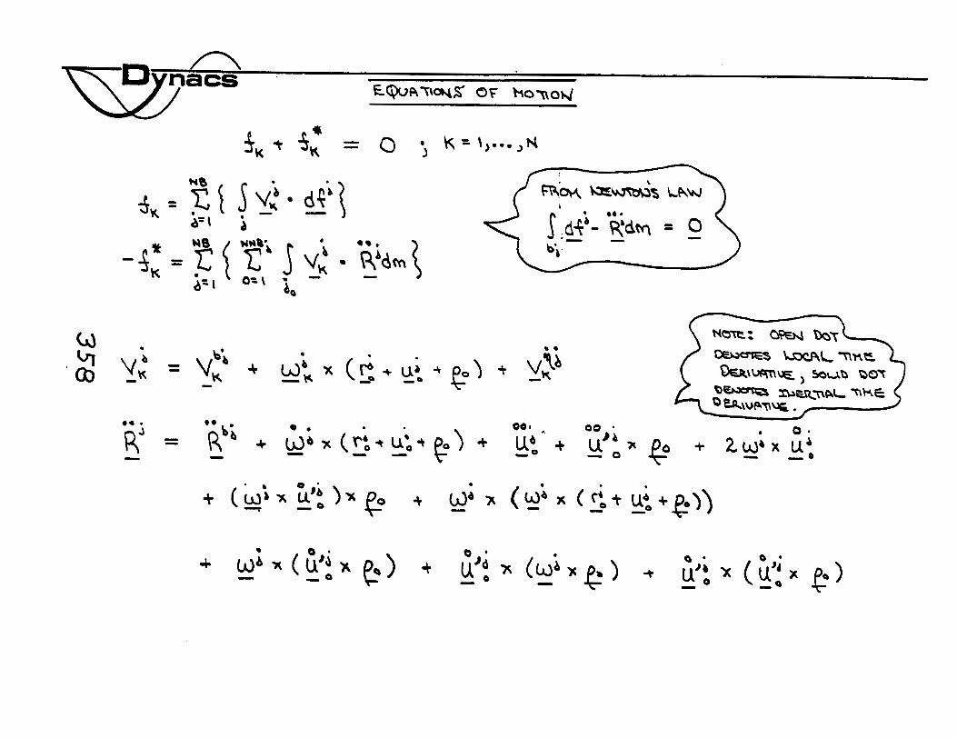


e_
362
v


EXPLICIT MODELING AND COMPUTATIONAL IDAD DISTRIBUTION FOR CONCURRENT PROCESSING SIMULATION OF TEE SPACE STATION
R Gluck TRW Space and Technology Group
Redondo Beach. California
ABSTRACT
Analytical slrnulatlon of the dynarnlcs/control Interaction of large space structures is essential during the design process as full-scale tests of these vehicles in the laboratory are impractical. Furthermore. the ope~xtlonal manifests of large space systems on-orbit may call for slgnlncant changes In their mass and stiliness distributions a s well a s for substantlal growth during the vehicles' Metlmes. and these can be stu fed only by analytical simulation. i 9
/' C~lrrent methodologies for simulating large space structures hpolve implicit mathematical models and solutions on serial digital computsrs. These methodologies requlre unacceptably long computer processing time and 'rbitant costs a s the models become larger and more complex. Potential orders-of-mztude reductions in slrnulatlon Ume and cost of multibody dynamic syste >can be attained using: (11 enhanced analytical models for simulation. and (2) sFcial-purpose. concurrent computational hardware apd system software.
6 (&:- ,Y , , : . cL:- I.WO Important aspects of concurrent processlng under development 0 thecderivaUon of explicit mathematical models of multibody
dynamic systems. and (21 a balanced computational load distribution (BCLD) among loosely coupled computational units (processors) of a concurrent processlng system. The developed methodologies w&&+demonstrated by way of an application to the Phase 1 of the Space Station - a task being performed by TRW under NASA/JSC contract NAS9- 17778. ,' ,,>
The malhemallcal model of the Space Station consists of three interconnected flexible bodies capable of undergoing large, rlgld-body motion with respect to each other. Body 1 is the main central body and contains the p r e ~ s u ~ e d modules inboard of the two Alpha
I gimbals. Bodles 2 and 3 are the starboard and port bodies connected to Body 1 at the Alpha , gimbals and include all components on the transverse booms outboard or the Alpha
gimbals (Including the solar arrays). The control systems in the model maintain Body 1 in a prescribed 3-axis attitude control mode, whlle producing large-angle rotations of the flexible solar arrays to position them normal to the sun-lint.
PREC6iDIffi PAGE BUNK NOT FLMED 371

The BCLD methodology for concurrent processing developed by TRW enploys a static allocation strategy in which a separate software package is used off-line and at leisure prior to the execution of the simulation program. The load distribution, in this methodology, is carried out in a manner transparent to the user who, nevertheless, exercises control over the procedure with pre-selected constraint conditions.
The distributed model of the Space Station is now complete and ready to undergo benchmark tests on TRW's Custom Architectured Parallel System during the June-July 1988 timeframe.


Introduction
This paper presents the application of concurrent processing technology developed at TRW Space & Technology Group over the past several years to the simulation of the Space Station. The effort is funded by NASA Johnson Space Center under Contract NAS9-17778 and monitored by Mr. John W. Sunkel. The period of performance extends from April 1987 to November 1988

OBJECTIVE
This project was established to provide NASA with quantitative data to determine the
cost effectiveness of utilizing a specialized processing system such as the Custom
Architectured Parallel Processing System (CAPPS) for development and verification of the
operational Space Station flight control system. The CAPPS is a concurrent processor
consisting of loosely coupled, high speed array processors [computational units (CUs)] - each containing its own input/output capability and memory banks. The specially designed
CUs are capable oE concurrent computation and communication, thereby placing a very low
overhead on the latter operation. Furthermore, the system's architecture provides for
direct communication between each CU and any other CU, facilitating considerable
flexibility in adapting the CAPPS architecture to a specific simulation problem.

Objective
The objective of this project is to develop, verify and demonstrate the simulation of an explicit model of the controls/structure interaction of the Space Station on CAPPS
Enghming & list Division T R W Spxr! & kchnolrwly G r w p
PROJECT WORK BREnKDOWN STRUCTURE
Applying previously developed application and system software at TRW to the
concurrent processing of an explicit model of the control/structure interaction of the
Space Station on CAPPS, the project described herein consists of three sequential tasks
as stated in the figure. This paper focuses on the completed Tasks (a) and ( b ) . Task
(c), at the time of this writing, is in progress.

Project Work Breakdown Structure
Enginaring & kt Division TRW Space & Wy Gra41
b. t 3. A Balanced Computational
Pmject r Load Distribution of Management the Space Station Model
for the CAPPS
c. v 4.
Simulation of ths Spm Station Model on the CAPPS


ADVANTAGES OF EXPLICIT EQUATIONS OF MOTION
The derivation of the equations of motion by symbol manipulation has several
important attributes compared to the conventional (implicit) methodology. Symbol
manipulation, i.e., the nonnumerical computation with a digital computer, yields scalar
equations of motion specifically tailored to complex dynamical systems, where the analyst
has the freedom and insight to incorporate any required fidelity in the model. Further-
more, the output of symbol manipulation is a completely portable FORTRAN code in the
format of A(x,t)G = b(x,tl, which can be delivered via file to either serial or concurrent
processors without requiring any programming. This reduces development cost by at least
one order-of-magnitude or more compared to that of a special-purpose implicit code.
Finally, symbolically derived scalar equations of motion require a substantially reduced
simulation time compared to those of conventional codes. Benchmark tests conducted at TRW
yielded improvements in run times by factors of approximately 4 and 3 for rigid-body and
LJ flexible-body systems, respectively.

Advantages of Explicit Equations of Motion
Engineering & k t Division TRW Space & Techrolny Gmlp
Useful engineering insights into the dynamic characteristics of the system
No major programming effort required to perform simulation
Large reduction of time required for simulation as compared to that required
I\, for implicit formulation a? - - Implicit formulation requires the derivation of the equations of
motion to be performed numerically at each integration step
- Explicit formulation requires the derivation to be performed only once

ADVANTAGES OF USING PROGRAM SMP TO DERIVE EXPLICIT EQUATIONS OF MOTION
Program SMP was selected for the TRW symbol manipulation methodology following a
thorough analysis which proved it superior in both versatility and speed to other
available symbol manipulation codes such as MACSYMA, Reduce and FORMAC. The SMP program
is implemented in the C language and is available on a variety of mainframes and work-
stations. Its capability of handling very large amounts of data is ideally suited for the
derivation of explicit equations of motion of muitibody spacecraft. The program's other
attributes are listed in the accompanying figure.


PROGRAM SYMBOD
Program SYMBOD for the derivation of the explicit equations of motion of multibody
flexible dynamical systems was developed within the general framework of SMP. A menu is
provided to the analyst for introducing the system's topology and appropriate logic is
available for the definition/computation of the essential elements of Kane's Dynarnical
Equations as shown ln the figure; however, the analyst can, at his discretion, override
the logic imbedded in each of the program's modules. The procedure is considered to be
optimal in the sense that it leaves with the analyst the tasks he is best trained to
perform, while transferring to the computer the manually prohibitive algebraic manipula-
tion and long derivation operations.
Two methodologies were incorporated in Program SYMBOD for dealing with the presence
of m geometrical and velocity constraints in a multibody dynamic system. In the first
Q methodology (by Wampler et al, Reference 1 1 , the dynamic equations governing a constraincd
system are generated symbolically directly from expressions comprising the equations
governing the system without constraints. This methodology for constraint elimination
(which requires a symbolic inversion of a matrix of order m) is applied when the number of
constraint equations in the system is small (m<6) and no working constraints are involved;
otherwise, the Lagrange multiplier methodology is used, where the stabilized penalty
procedure of Reference 2 offers an attractive way for stabilizing the constraint equations
now retained in the mathematical model.

-
€ .g
ms
L
cn =-
mu
m
.II -0
Ern
s
e-
= g*
- E*
go
E
fu Q
)W
L
&b
$
E =
0 fuc
F=
u
ATTRIBUTES OF P H O G W SYMBOD
Program SYMBOD contains several innovations which combine to produce an eEficient
mathematical model. These are listed in the figure and explained briefly below.
The generation of equations of motion by symbol manipulation requires a systematic
method of reducing the number of algebraic operations in the formation of Kane's
equations. Frequently, the intermediate computations of expressions, such as the velocity
terms, produce a multitude of expressions so large that their storaqe requirements exceed
the computer's capacity. A procedure for systematically introducing new intermediate
symbols to replace recurring combinations of algebraic subexpressions was developed. This
procedure eliminates repetitious calculations and results in efficient computational
algorithms requiring fewer arithmetic operations.
The formulation of Kane's dynamical equations associated with the flexible-body
degrees-of-freedom (dof) of a body are iterative in the number of assumed admissible
functions required to represent the flexibility. The totality of the flexible-body dof
for each body was, therefore, represented in Program SYMBOD by a single dof of that body.
This allows postponement of the final selection of the required number of assumed
admissible functions until after the development of the explicit mathematical model
(including the control system) is completed, i.e., the assumed admissible functions in
this formulation need not be selected prematurely.
Program SYMBOD provides for direct elimination (by command) of superfluous higher
order terms in the explicit equations of motion when these terms are inconsistent with
basic assumptions made in the formulation or with the variance of input parameters.


ElqifdaJ&bstOivisiarr I-FW Space Techdorly G ~ N Q
The Space Station Model Contents (A joint effort of NASA & TRW)


a C a
4
4
0
3 u
a, E
u
iu
0
a
&
a 0
n C
-4
m a, 4 3
a
0
E
a
a, N
-4
L 3
ffl rn a, &
a
a, x
u
m C -4
n; u
C
0
U
a
C
([I
X
a
0 n
4
a
k
u
C 0
U
C
.4
5
E
a, .c u
m
. rl
al L: u
u
([I
7
X
m
0
m
0 u
a
aJ u
U
a, C c 0
U
m a, - 4
a
0
n u
&
0 a
a
C
a a
k
m 0 a
&
([I u
ffl
a, C
u
a, k
n3
m
a C a
N
m
aJ .4
a 0
m m
rl
a
P
E
.4
CT
X
a
0
n I
'U
. rl u' -4
k
* C
0
.rl
u
0
f a' D'
k
([I 4
0)
- L, E u' .d
a,
ffl C
-4
a
u
C
0
U
.-I a,
0
E
C
0
.4
u
a
u
cn aJ U
a a
V]
X
a 0 P I
a! aJ L
z
4J
aJ L: b
tr, C
.4
rl 0. 3
0
U
4
4
3
G4
X
a 0
n
4
a
k
u
C
a, U
a, L
u
0
u
a, > . 4
u
ffi rl aJ k
rn '3 .4
a 0 P
m 3 0
aJ C
a h 3
X
C)
aJ s
C1
cu 0
E
U
a
C)
k 0
rr
4
a
C
0
.4
u
a
u
0
k

FREQUENCY SPECTRA OF THE SPACE STATION MODEL
The assumed admissible functions in the Space Station model were obtained from finite
element models developed for each of the bodies. These included an unconstrained (free-
free) model for the central body and two constrained (fixed-free) models for the starboard
and port bodies, cantilevered at the Alpha gimbals. A MSC/NASTRAN code was used to obtain
the natural modes of vibration within a 10 Hz frequency bandwidth. The spectrum of
natural frequencies for each of the three finite element models is shown in the figure.
Note that these are characterized by a number of low frequency modes (below 1 l l z ) spaced
closely together.


ATTIel'UDE CONTROL S Y S T E n FOR S P A C E S T A T I O N MODEL
The attitude control system of the Space Station was designed to regulate its
orientation and keep its longitudinal axis aligned with the local vertical vector while
maintaining its plane perpendicular to the velocity vector. The control system consists
of attitude sensing instrumentation, control moment gyros, and electronics to cause
corrective control moments to be applied to the Space Station's central body whenever it
moves away from the commanded attitude. The attitude and rate sensors and the control
moment gyros (CMG'sl are co-located at the origin of the coordinate system of the central
body placed at its undeformed center of mass.
A block diagram of the control law for the X2 axis is shown in the fiqure. Similar
control laws were designed for the remaining two axes (the three control laws are un-
coupled from each other). Attitude sensing instrumentation provides electronic represen-
tations of the attitude angle 82 and its time rate of change. The sensed attitude angle
is subtracted from the commanded attitude angle 102c) to form the attitude error signal
a (82e). The electronic controller mechanizes a control law, specified in the form of a
transfer function, to produce a commanded control moment (MzCI based on the error signal.
The CMG generates control moments (M2) according to the commanded moments to drive the
attitude error towards zero. External disturbances are not considered in this simulation
and the commanded attitude is set nominally to zero.


ART ICUIATED- BODY CONTROL FOR SPACE STATION MODEL
In addition to the attitude control system, the Space Station model includes a second
control system to maintain the solar arrays pointing in a direction perpendicular to the
sun line. The control law is based on an angular position and rate feedback scheme with
options provided to rewind the solar arrays during eclipse. The commanded angular
position of the Alpha gimbal is utilized in a second order transfer function to calculntc
the controller's motor torque. Input and output parameters for the articulated body
control system are shown in the figure.

Articulated-Body Control for Space Station Model
Enginariq&'T;cstDivisiorr TRW Space & l ihrdnqy Gmp
- Joint Angles & Rates - I I Joint Drive Torques -
- Joint Rate Commands - I I-- - Unit Sun Vector I
Position, Velocity, Body Rates - & Body to Inertial Frame
Transformation --I Articulated Body Control Subsystem
- Time 1
Joint Angle Status Flags, - Joint Angles, Rates & -
Accelerations
- Measured Joint Angles & Rates -r-
Source: Mr. J. Mapor, LEMSCO; Houston, Texas


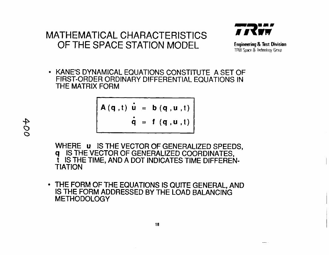
MATHEMATICAL CHARACTERISTICS OF THE SPACE STATION MODEL Engineering & Test Division
TRW Spac~! & Techbqy Grrn~p
KANES DYNAMICAL EQUATIONS CONSTITUTE A SET OF FIRST-ORDER ORDINARY DIFFERENTIAL EQUATIONS IN THE MATRIX FORM
WHERE u IS THE VECTOR OF GENERALIZED SPEEDS, q IS THE VECTOR OF GENERALIZED COORDINATES, t IS THE TIME, AND A DOT INDICATES TIME DIFFEREN- TIATION
THE FORM OF THE EQUATIONS IS QUITE GENERAL, AND IS THE FORM ADDRESSED BY THE LOAD BALANCING METHODOLOGY
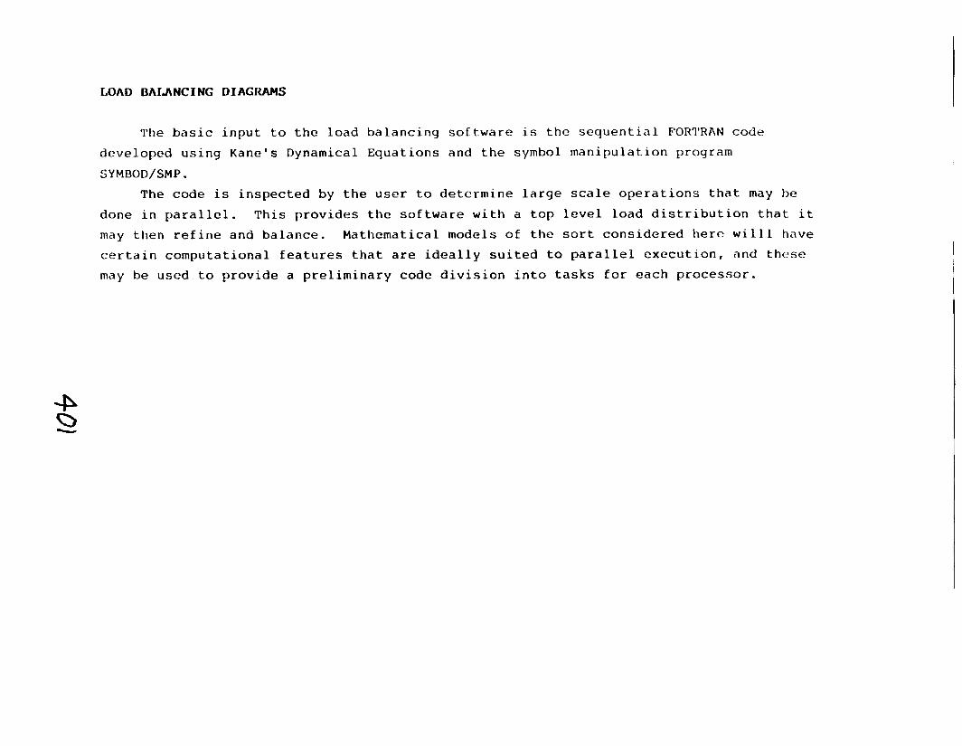
LOAD BAIANCING D I A G I W S
The basic input to the load balancing software is the sequential FORTRAN code
developed using Kane's Dynamical Equations and the symbol manipulation program
SYMBOD/SMP.
The code is inspected by the user to determine large scale operations that may he
done in parallel. This provides the software with a top level load distribution that it
may then refine and balance. Mathematical models of the sort considered here will1 have
certain computational features that are ideally suited to parallel execution, and these
may be used to provide a preliminary code division into tasks for each processor.

LOAD BALANCING DIAGRAMS
I CODE I A I APPLY TOP LEVEL
LOAD DlSTRlBUTtON I
TO PROCESSORS
Engineering & %st Division TIW $act & Technnlrqy Gram

LOAD DALANCING DIAGRAMS (CONT'D)
The code is then divided into smaller tasks using the program TASK. This parti-
tioning incorporates the divisions already given in the top level distribution, and
results in tasks which are no smaller in size than some predetermined "grain" size. The
user chooses whether or not the code division is to be fine-grained or coarse-grained.
Different choices will be a result of, e.g., a different number of available processors,
the need to examine values for intermediate variables in a convenient way, etc.
Once tasks are obtained, TASK checks to see that the size and execution time for
tasks that are to be executed in parallel are approximately the same (according to
criteria determined, in part, by the user), in order to have a balanced computational
load. Those tasks found to be too large are divided while those that are too small are
merged with tasks to be executed before or afterwards. This division and merging
continues until the criteria mentioned above are satisfied.

LOAD BALANCING DIAGRAMS
(CONTINUED)
( DETERMINE GRAM SlZE 1
DIVIDE CODE INTO SEGMENTS (TASKS) NO SMALLER THAN ( THE GRAIN SIZE (SUBJECT TO TOP LEVEL LOAD DISTRIBUTION)
I I OBTAIN SIZING AND TIMING INFORMATION I I I
RETURN P,
TASKS TO BE A PA. - -,
HAVE APPROXIMATE1 THE SAME SlZE AND
EXECUTION .
MERGE CONSECUTIVE TASKS THAT ARE TOO SMALL; DIVIDE TASKS THAT ARE TOO LARGE

LOAD BATANCING DIAGRAMS (CONT'D)
At the conclusion of the code division, the tasks are evaluated in terms of how much
communication they require with other tasks, and how many variables and parameters they
share with other tasks. The program ASSIGN takes the results of the first of these
evaluations and constructs what is called the connectivity matrix, with each entry
indicating how much communication from task S, say, to task T is required, where S and T
range over all tasks. ASSIGN uses the second evaluation to produce the parametcr overlap
matrix, where each entry indicates the number of parameters shared by the two tasks.
Tasks to be executed in parallel are now assigned to processors by ASSIGN. The
connectivity and parameter overlap of each task with tasks already assigned to the
processors is examined and a task is assigned to a particular processor according to a
set of previously specified constraints.
At the end of the assignments, ASSIGN checks the computational load for balance among
the processors. If the result is acceptable, then the software is finished. If not, then
the constraints may be relaxed (in a way predefined by the user) and task assignment may
0 be attempted again. If the constraints have been relaxed as far as possible, and the load
is still not acceptably balanced, then TASK will attempt a different code division (and
subsequent task assignment using ASSIGN) where the grain size may be different than
be fore.
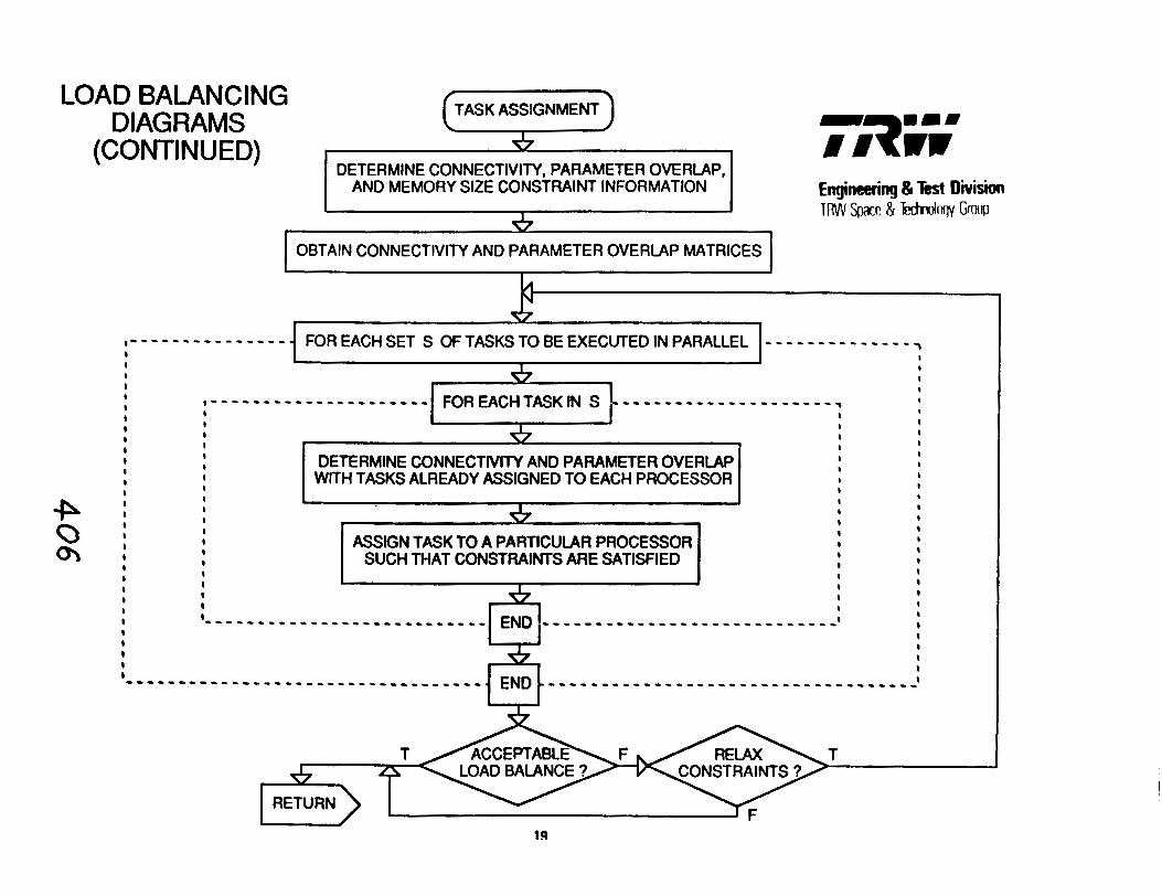
LOAD BALANCING DIAGRAMS
(CONTINUED) \ J -
DETERMINE CONNECTIVITY, PARAMETER OVERLAP, 1 I?;;
AND MEMORY SIZE CONSTRAINT INFORMATION Engineering & k t Diivi~i~n Tn\FJ Space! & Tedmlrr~y Graq
OBTAIN CONNECTIVITY AND PARAMETER OVERLAP MATRICES .
. DETERMINE CONNECTIVITY AND PARAMETER OVERIAP WITH TASKS ALREADY ASSIGNED TO EACH PROCESSOR
I - - - - - - - - - - - - - - - -
I
I 8
.P j I I
1 I I
I I I
I t
o b I I I ASSIGN TASK TO A PARTICULAR PROCESSOR I I
I I
I
OI 8 I I
I SUCH THAT CONSTRAINTS ARE SATISFIED I
I I I
I
I I I
I
I I t
I
I I
I I
I
I I I
I - - - - - - - - - - - - - - - - - - - - - - - - - - - END - - - - - - - - - - - - - - - - - - - - - - - - - - - - I I I
I I
I I
I I I '_ - - - - - -_- - - - - - - -_- - - - - - - - - - - - - - - - - . . . . . . . . . . . . . . . . . . . . . . . . . . . . . . . . . . . I
FOREACHSET S OFTASKSTOBEEXECUTEDINPARALLEL - - - - - - - - - - - - - -
T T
RETURN
I
7
I
I
I
I
I
I I
I I - - - - - - - - - - - - - - - - - - - - - FOREACHTASKlN S ---------------------,
I I
I
I I I
I
I

DATA FIaOW GRAPH
The data dependencies in the Space Station model are shown in the figure. The graph
depicts the functional form of the model's equations.
The state vector, En, at a given time tn is composed of the generalized speeds (!,I,
the generalized coordinates (qn) and the control variables ( ~ ~ 1 .
The generalized coordinates are used in calculating time derivatives for all the
state variables, as are the generalized speeds (though these are not used in the computa-
tion of the matrix fin). The control variables affect only the control torques and thus
influence only the vector bn and the derivative of LIn. Time derivatives of CJn and cn are found directly from the generalized coordinates and
speeds. Gaussian elimination is used to solve the matrix equation fin Gn = En giving the derivative of En.
The time derivatives of each of the components of the state vector are collected to
give the derivative of xn. This is then integrated using the Adams-Bashforth algorithm to
give the state vector at time tn+l:~+l.
P 0 -4

DATA FLOW GRAPH
\ / ALGORITHM
ADAMS-BASHFORTH ALGORITHM

TOP LEVEL LOAD BALANCING (SPACE STATION MODEL)
Some opportunities for parallel execution of the Space Station model code are
immediately apparent from even a casual inspection of the model, as shown in the figure.
The coordinate transformation matrices between frames in the three bodies, and
between the body frames and an inertial frame are used frequently and must be calculated
first. Each matrix, however, is calculated by a processor only if that processor will
subsequently use it.
The outputs of the control subroutine are used only in the computation of the vector
b. Thus, this subroutine may be executed in parallel with sections of code computing -
general intermediate variables used by both fi and b (such as partial angular velocities, partial velocities, etc.).
The calculation of elements of - A and b may also be done in parallel, as may be the computation of the time derivative of q.
A general division of the code may also be made according to whether computations
involving Body 2 or Body 3 are needed. When possible, therefore, a given processor will
compute quantities related only to Body 2 or only to Body 3, thus reducing interprocessor
communication.

TOP LEVEL LOAD BALANCING (SPACE STATION MODEL) Engineering 81 Test O~sion
TRW Space & Tednoloqy Gro~ lp
COORDINATE TRANSFORMATIONS
CONTROL GENERAL SUBROUTINE
INTERMEDIATE VARIABLES
FORCES, TORQUES
INTERMEDIATE INTERMEDIATE VARIABLES FOR VARIABLES FOR
A b
A b
2 1

AN OVERVIEW OF TIIE CAPPS SIMULATION METHODOLOGY
An overview of the CAPPS simulation methodology is shown in the figure. The
methodology is divided into four phases. The analysis phase constitutes the development
of the mathematical model and requires an intensive interaction between the analyst and
the previously described Program SYMBOD/SMp. The derivation phase follows, in which
Program SMP carries out the instructions imbedded in SYMBOD to yield a matrix of ordinary
differential equations in FORTRAN format. In addition to providing an accurate reflection
of the analyst's intentions in the derivation of the equations of motion, this procedure
also leads to equations which are virtually free of wasteful operations (such as additions
of zeros, multiplications by unity and taking dot products of orthogonal vectors), as well
as superfluous high order terms. The FORTRAN equations are delivered via file to the
CAPPS computational load distribution software to begin the processing phase which is
described in more detail below. It should be noted that the procedure completely
eliminates the costly and time consuming programming effort which is normally required at
4 this stage. The CAPPS system software transforms the derived equations from their - - original FORTRAN format to a binary format executable in concurrent operations by the CAPPS's CUs.
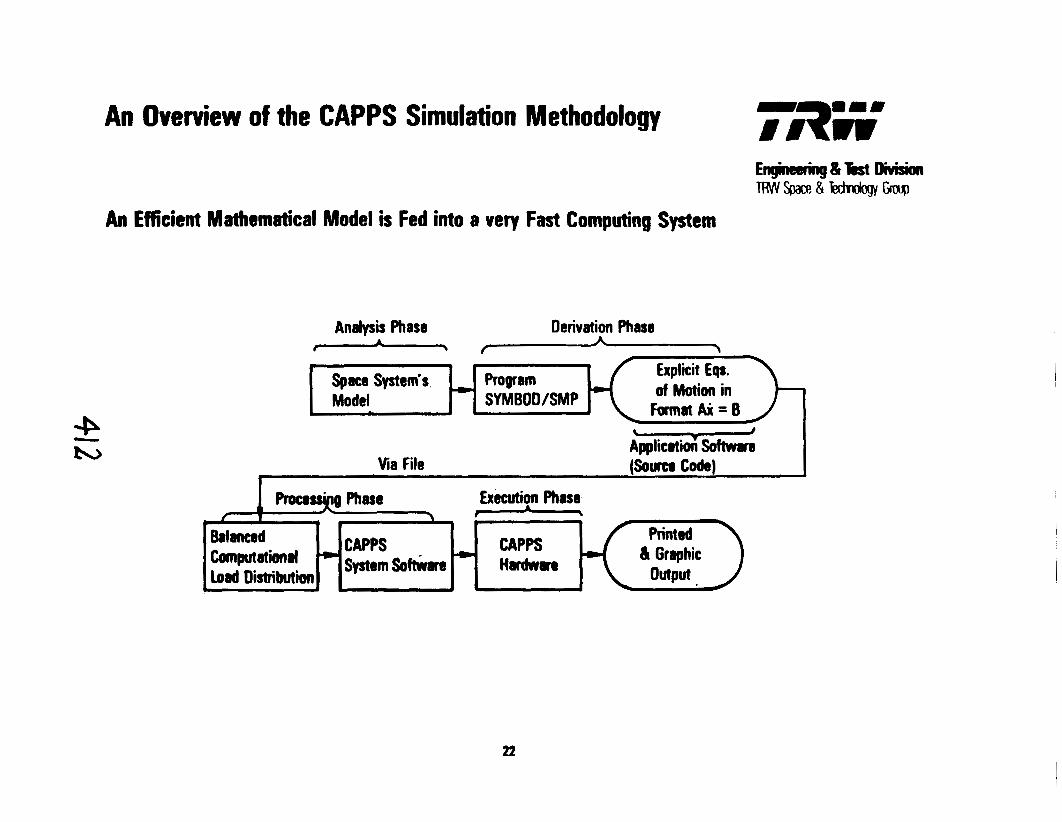
An Overview of the CAPPS Simulation Methodology
Engineering & kt Divisian TwSpace&mGrcrrp
An Efficient Msthernatical Model is Fed into a very Fast Computing System
Analysis Phase Derivation Phase
Via File ($w Code) r I
- s 1
Program Explicit Eqt,
SYMBOD/SMP of Motion in
J
Prowssg Phase Execution Phase 1 \ -
FmnaAi=B
Space System's, Model
A
Balanced Com~u'"'m" Load Distribution
-
.r
8
CAPPS swem s o h . .
- CAPPS Hadwat41

REFERENCES
( 1 ) C. Wampler, K. Buffinton, and J. Shu-hui, "Formulation of Equations of Motion for
Systems Subject to Constraints"; ASME Journal of Applied Mechanics, Vol. 52, June
1985.
( 2 ) K. C. Park and J. C. Chiou, "Stabilization of Computational Procedures for
Constrained Dynamical Systemsw; University of Colorado, College of Engineering,
Report No. Cu-CSSC-87-05, June 1987.

SIMULATION OF FLEXIBLE STRUCTURES WITH IMPACT: EXPERIMENTAL VALIDATION
A. Calip Ulsoy University of Michigan Ann Arbor. Michigan
ABSTRACT
The dynamics of flexlble systems, such as mechanisms and robotic manipulators, b becoming Increasingly important due to high-speed operation, high accuracy requirements, and Ilghtwelght designs. Such flexible devlces can undergo impact during operation, and this may lead to: (1) component faflure due to high stresses. and (2) excitation of higher structural modes due to impulsive forces. The latter issue. the slrnulatlon of the dynarnlc behavior of flexible structures with impact. is cxperlmentally and numerically investigated.
A radially rotating flexible beam attached to a rlgld shaft is considered. Both experimental and numerical studies are undertaken. Experlrnental studies show excellent agreement with simulation studles uslng both the momentum balance [ct~fllclent of friction). and spring-dashpot (impact pair) models. The simulation sl~rdies are even capable of predicting Ule hlgh-speed multiple impacts which occur due lo structural flexiblllty and which were experlrnentally observed using huh-speed video photography. The results of the studies show that a simple momentum balance (coclTlclent of restitution) method for simulating the Impact I s sufficiently accurate in predlctlng the dynamic behavior of the system for most engineerlng applications. The momentum balance method cannot simulate the impact force whlch develops during the conlact duration. but is compulationally very emclent. The spring-dashpot model I s more dimcult to develop and requires slgnlficantly larger computation tlrne, but can slnlulate lrnpact forces and stresses due to Lmpact.
The momentum balance (coefficient of restitution) method, although strlctly not applicable to flexlble bodles, has been shown to provide an accurate and computationally emclent method for simulating the dynamic behavior of flexible slruclures with impact when contacl stresses are not needed.
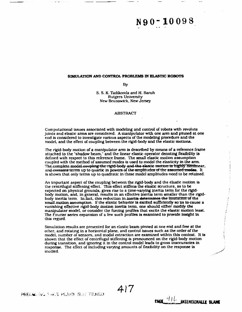
SIMULATION AM) CONTROL PROBLEMS M ELASTIC R O m
BY
S. S. K. Tadtkonda and H. Baruh Rutgers University
New Brunswick. New Jersey
ABSTRACT
Computational issues associated wlth modeling and control of robots wlth revolute joints and elastic arms are consldered, A manipulator wlth one arm and pinned at one end is consldered to InvestJgate various aspects of the modellng procedure and the model. and the eITect of coupling between the rigid-body and the elastic motlons.
'fie %id-body motion of a manipulator arm is described by means of' a reference frame attached to the "shadow beam." and the linear elastic operator denoting flexibility Is defined wlth respect to this reference frame. The small elastic motlon assumption coupled wlth the method of assumed modes Is used to model the elasticity in the arm.
t d - b o d y m & h e . ~ l e amthn-ear. *powers of' t t x a m p i i t a . It Is shown that only terms up to quadratic in these model amplitudes need to be retained.
I An Important aspect of the coupling between the rigid-body and the elastic motion is I
the centrifugal stiffening efrect. This efTect stlITens the elastlc structure. a s to be I
expected on physical grounds, ghres rise to a time-varying @ertia term for the a i d - /
body motion. and. in general, results in an eITectlve inertia term smaller than the rigid- body inertia term. In Zart. thls reduction frrlnerusl.&- +he-tfie (
sm;rllmoUoa ~ssurnptlon. If the elastic behavfor is excited 8dllclently so-as tocause a vanishing enective rigld-body mollon inertia tern, one should either modlfL the I manipulator model, or consider the forcing profiles that excite the elastic motion least. I I 'The Fourler series expansion of a few such profiles I s acamfned to prwide lnsfght ln thLs regard.
1
Simulation results are presented for an elastic beam plnned at one end and free at the 01 her. and rotating in a horizontal plane. and control Issues such as the order of the model, number of sensors. and modal extraction are examined wlthin this context. It is shown that the effect of centrifugal stlllenlng is pronounced on the rlgld-body motion I
durlng transltion. and ignoring it In the control model leads to gross inaccuracies in response. The effect of including varying amounts of flexlbllity on the response is sludled. + ,. A

SIMULATION AND CONTROL PROBLEMS
IN ELASTIC ROBOTS
Mechanical & Aerospace Engineering Dept., Rutgers University, New Brunswick, NJ.
* Graduate Assistant
** Assistant Professor

OBJECTIVE
To investigate modeling, control, and computational issues associ- ated with elastic manipulators
SCOPE
Revolute joints
Actuators at joints only
Shadow beam approach
Small elastic motion, and limit of such an assumption
Nonlinear model
Control issues
Illustrative example

Pinned - free link
Reference frame located at the pin joint; describes rigid-body motion. Elastic motion is defined with respect to this frame
Notes: x is the position of the point in the undeformed configuration The beam rotates in a horizontal plane

u(x,t) is obtained by integrating
where q(x,t) = x + s(x,t)
<(x,t) = x - u(x,t)
On integration,
s(x, t) : axial vibration term
Integral : results in centrifugal stiffening term
Neglect axial vibration

- 5 -
Elas tic Displacement
Position
Velocity
Kinetic Energy
Potential Energy
Lagrangian
Notes : ( ) corresponds to partial derivative with respect to time. ( )' corresponds to spatial derivative, p is the mass per unit length. and EI(x) is the
flexural rigidity

Assumed Modes
Q i ( ~ ) : Admissible functions

Define
L kij = Jo EI(X) q f (x) $;(x) dx
Then,

Substituting in the Lagrangian,
Example : Beam parameters
Cross-section : 6 in x 31 8 in Length = 3.6576 m (12 ft) p = 4.015kg/m EI = 756.65 N . m
Admissible functions : Normalized eigenfunctions of a pinned-free beam
where 6 i is the Kronecker delta Notes : The surkrnarion convention, C Z m i j ai aj = mij ai aj, etc., will be em- ployed for conciseness - i.e., repeated indices in an expresslon indicate summa-
tion over appropriate range.

- 9 - Natural frequencies and Centrifugal stiffening coefficients
Coriolis terms, qijk
Other coupling terms sijkl
Note: Sijkl = Sj&l = Sijlk = Sjilk
i oi
+
Pij
1 j = 3
-0.366 6.195 35.999
. 1 2 3
j = 1 I j = 2
15.82 51.282 106.983
6.397 1.861
-0.366 .'
1.861 17.905 6.195

Notes : The magnitudes of the terms qijk and s,jkl are sma!l. In addition, they are multiplied by the cubic and quartic powers o f modal amplitudes. Hence they will be dropped from further development.

Retaining terms only up to quadratic in modal amplitudes,
' 2 . . L= 112 [I,- (pij - mij) ai aj] 8 + 112 mij ai aj
- 112 kij ai aj
The equation for rigid-body motion is
And the elastic motion is described by
' 2 mij aj + [kij + (pij - mij) 8 1 aj - - T @i'(o),
i = 1, 2, ....., N1
Measurements at x = 0
= 8 + ~ ' ( 0 , t )
. I
el = 8 + v(O,t)

- 12 -
Choices for the control model
1 . Ignore elastic effects completely . .
Control model : I, 8 = T . 8 = el 8 = 8,
2. Rigid-body model, with the sha- dow frame angle properly extracted
Control model : I, 0 = T 0 = 8, - ~'(0,t) 8 = 8, - C'(0,t)
3. A few elastic modes are included, and the modal coordi- nates are approximated
Control model:
Notes : N1 is the number of modeled modes. N2 is the number of modes used for controller design. NI = 3 for the following simulation results.

4. A ~ ~ r o ~ r i a t e number of sensors uskd io obtain accurate modal coordinates.
Control synthesis
Computed torque method
Pointwise-optim a1 control method

- 14 - Open-loop Maneuver
100.0-
75.0-
50.0-
T' 25.0. I z - 0.04 U 3
F s -25.0-
-50.0.
- n . o .
-1oo.oC ? 0.0 0.1 0 2 0.3 0.4 0.5 0.0 0.7 0.8 0.9 1.0
rime (s)
Fig. 1 : Torque Profile for Open-Loop Maneuver
0.10-
- Flexibility included
- - - , , Flexibility neglected 0.08.
0.00.
: a a 0.04.
0.02.
0.0 0.1 0.2 0 . 3 0.4 0.5 0.6 0.7 0.8 0.0 1.0 time (s)
Fig. 2 : Position Response of the Beam for the Torque Above
432

Feedback Control
Fig. 3 : Rigid Model, Velocity response
A - Actual velocity
1 , , , , , Desired velocity I
Time (s)
Fig. 4 : One Flexible Mode Included in the Model
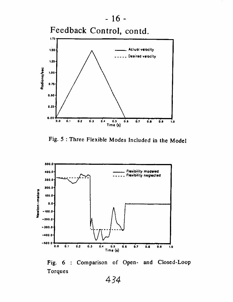
- 16 - Feedback Control, con td.
- Aclual velocity h - - ! - - A . -.--.A
Fig. 5 : Three Flexible Modes Included in the Model
Fig. 6 : Comparison of Open- and Closed-Loop
bOO.0
400.0-
100.0-
aoo.0-
t r 100.0.
i I C
0.0- 0 -
-100.0-
: -100.0-
-100.0.
400.0-
-500.01;
Torques
0.0 0.1 02 0.3 0.4 0.5 0.1 0.7 0.a 0.a 1.0 Time (s)
- Flexibility modeled - - , , , Flexibility neglected
i

Effects of centrifugal stiffening
1. Provides a strong coupling between the rigid-body and elastic motion
2. Increases the stiffness of the struc- ture
3. Reduces the effective rigid-body inertia term. Can cause it to vanish if the elastic motion is large. May have to modify the model, or vary the torque profiles.

Torque profiles and their Fourier coefficients
coefficienfs of

Computational Issues for Control of multi-link flexible robot arm
1. The dynamic model can be arrived at by modeling each link indepen- dently and imposing constraints at the joints
2. The link geometry may not be sim- ple
Sijkly qijky may not be negligible, and the control model may include all the terms
4. The choice of admissible functions for each of the links may be different
5. Sampling rates - should not excite elastic motion
6. Control input computation may pose form idable burden.

The above issues can be adequately addressed by selecting pointwise- optimal control law for control input computations, where, the inputs can be computed at least one time step ahead.

Conclusions
1. A complete model for control of a flexible link is developed
2. Modeling issues are examined within the context of an example
3. Several control issues are investi- gated
4. It is shown that centrifugal stiffening effect on rigid-body motion is significant
5. There is a strong coupling between rigid-body and elastic motions; ignoring this coupling results in gross inaccuracies in response.

LPlEARIZED MODEL8 IN MULTXBODY DYNAMICS AND CONTItOL
Wllliam W. Clmino Boelng Aerospace
Seattle. Washington
ABSTRACT
w s slrnulation of structural response of m~lti-flacible~body systems by llnearked flexibre motlon comblned with nonlinear rigld motion/ Advantages and appllcabllity of such an approach for accurate simulation with greatly rcduced computational costs and turnaround times arc described. restricting attention , lo the control deslgn environment. Requirements for updating the I lnearhd flexlbillty model Lo track large angular motions arc discussed. Validation of such an approach by comparbon with other existing codes !s included. Applkatlon to a flexible
t robot manipulator system 1s described.
PR1EGPDCNG PAGE BUNK NOT FILMED
441

Linearized Flexibility Models in Multibody Dynamics and Control
12 July 1988
William W. Cimino
Boeing Aerospace Seattle, Washington

Some controls requirements of multibody codes
Introduction to SADACS
-b Validation P bJ Applications
Spacecraft
Robot manipulators

Some Controls Requirements
1) General purpose dynamic module
2) Models can be merged in any configuration without creating new structural models
3) Very fast (computationally inexpensive) Short simulation turnover time
- Time domain analysis with nonlinear controllers Sensitivity studies Stability analysis
Control design iteration

c 0
'LI
C,
a
d
B 'LI cn

SADACS is designed for controls environment
Used as general purpose dynamics module in a control simulation environment
Allows multibody systems to be merged in any desired configuration without creating new structural models
Very fast (computationally inexpensive) for system design and sensitivity/stability analysis
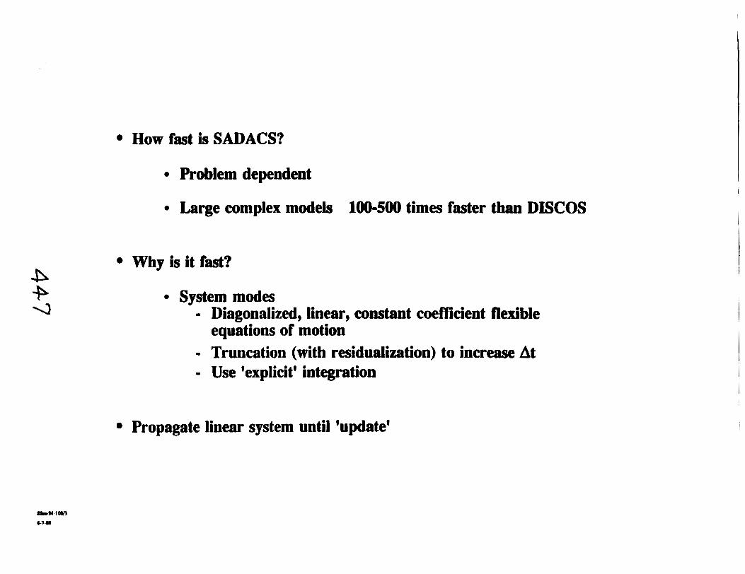

CPU Time Comparisons for 3-Body Problem
Other Test Problems : High Speed Simulation of Flexible Mulitbody Dynamics
Presented at MSFC, April 22-24, 1986
REMARKS
No component modal truncation
With component modal truncation
With system modal truncation
I
CODE
DISCOS
IIISCOS
SADACS
RUN TIMES
> 26 hours
5 hours 9 minutes
10 minutes
CODE
DISCOS
SADACS
RUN TIMES
OL SO Hours - 15 minutes
REMARKS
With component modal truncation
With system modal truncation

Multi-Flexible-Body Run- Times 3-Body simulation CPU (se6onds) I Real-Time (seconds)
DISCOS 0 TREETOPS
SADACS 0 Real-lime 1:l ----
Date of availability within Boeing Company

SADACS Structure
1) Nonlinear rigid body code (SDIEXACT, TREETOPS, MBDYN, etc.)
2) Linear flexible dpamics
System mode formulation
Retain truncated modes quasi-statically
3) System mode updatdrestart

Simplified Diagram of the SADACS Code
Inputs to the system (generalized forces and torques) are applied to both the rigid and flex motion solvers. The rigid motion solver computes the nonlinear rigid body response. The flex motion solver uses a "system mode" formulation to compute the linearized flexible response. The outputs are combined in the motion summer and tested for an "update condition". If an update is not required the outputs are passed out to the simulation. If an update is required, a new eigensolution is performed on the new configuration and the mode shapes, frequencies, and system mode state vector are adjusted.


Updating Time-Line Overview
A fixed modal set is maintained during a given epoch (time between updates). At the end of the current epoch the pre-update states are known. Following the eigensolution on the new system matrices, the new modes shapes and frequencies are known. The difficult part of the update is then to assign new values to the post-update states.

THIS PAGE INTENTIONALLY LEFT BLANK


Why is updating a problem?
When gimbal rotations and rates (which include structural deformations) developed in one configuration are imposed on a new configuration, they excite the structure in shapes (modes) that would not have occurred in a 'continuous' solution, and in addition fail to preserve energy.
The problem is nonlinearity-induced trading of excitation, or coupling, between the modes.

Example problem: chosen to emphasize 'trade' in modal participation
Want update that
1) Doesn't ring
2) Maintains energy
3) Tracks frequencies
4) Correct shapes
Coupling of flex into rigid neglected
- SADACS not intended for problems where flex nonlinearities drive rigid motion
Address update entirely with component modal variables

Example Problem
T h i s f i g u r e shows t h e sys tem used t o examine t h e upda t e . The sys tem h a s two f l e x i b l e modes w i t h c o o r d i n a t e s ql ( s o f t mode) and q2 ( s t i f f mode) .


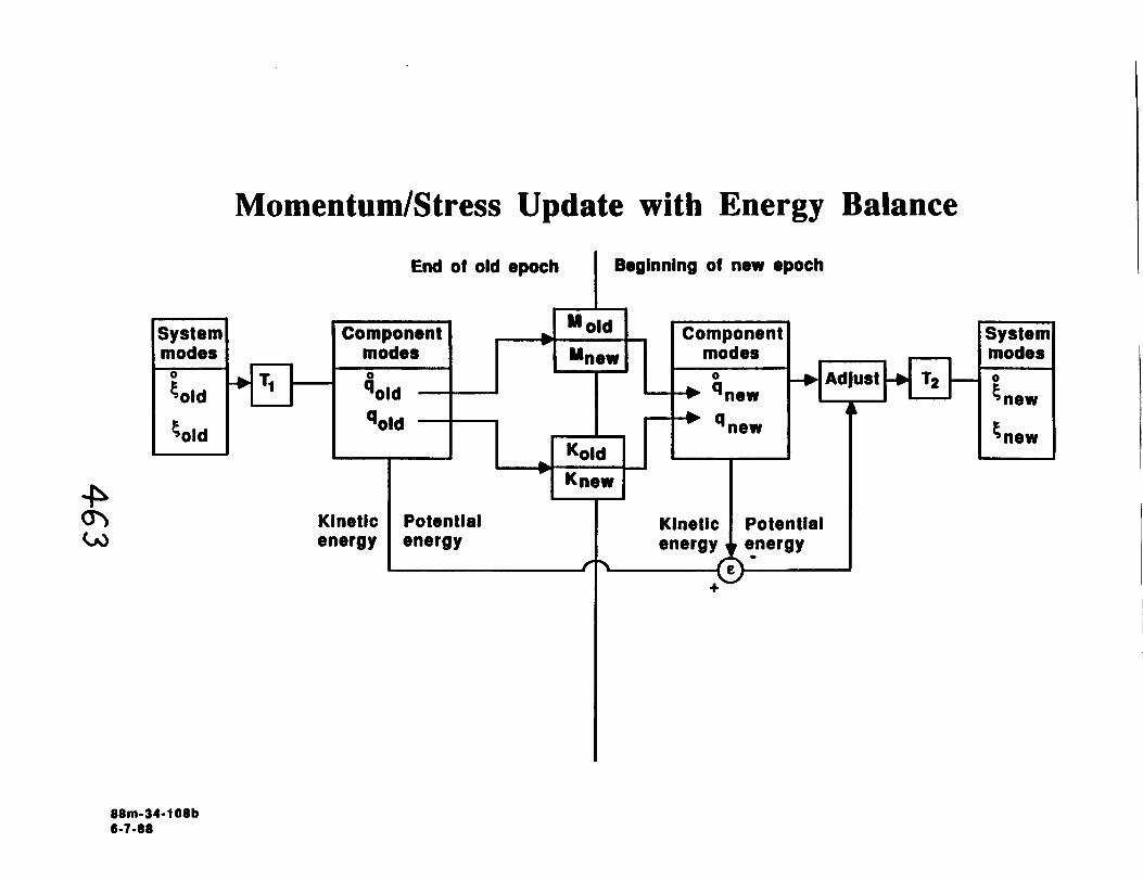
Momentum/Stress Update with Energy Balance
End of old epoch I Boglnnlng of new epoch
- 1
- System modes
0
cold
told
P Knew
rn Klnetlc Potential Klnetic Potentlal bd energy energy
f\
System modes 0
cnew
h e w
Component v old Component modes h e w modes .
TI T2 - . 0 + Adjust + - -b i(o~d b qnew
A qo~d qnew
Kold


SADACS program capabilities Summary
Rigid body analyser based upon the code used ( MBDYN, TREETOPS, SDIEXACT etc )
p. Flex body analyser ( FB2 )
Number of bodies no limit Number of flexural modeslbody no limit Number of gimbals no limit
Configurations : cluster linked tree closed loop manipulator multiple closed loop multiply grounded manipulator
Degrees of freedom at gimbals 0 - 6 ( totally locked to totally free )
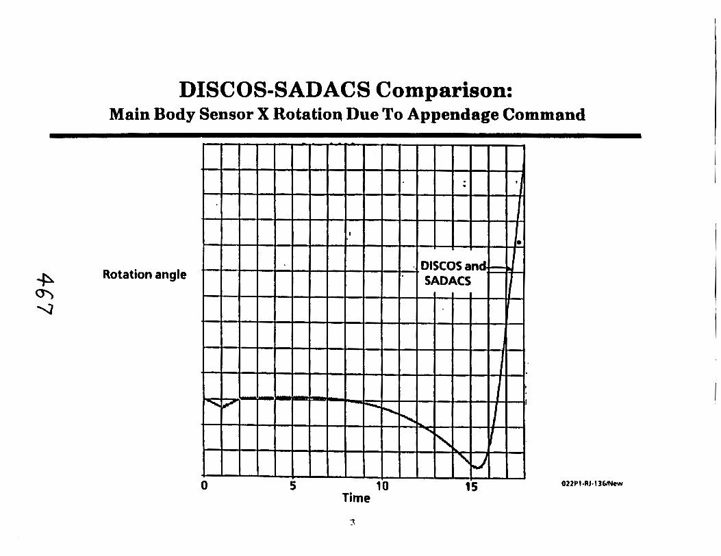

DISCOS-SADACS Comparison: Main Body Sensor X Rotation Due To Appendage Command

Controller Comparison - Closed Loop
The figure below shows the closed-loop response of a flexible model of the SPAR robot manipulator with three different controllers. The top plot is the first joint angle (waist) and the bottom plot is the z motion of the end-effector (up and down). The three different controllers are feedforward, semi-adaptive gain, and fixed gain.


Applicability
Large body of common problems
Problems not dominated by nonlinear flexible response
Each new problem should be validated against 'full code' (TREETOPS/DISCOS)

Conclusions
SADACS fast, ef'ficient multi-flexible-body simulation code
Designed for use in contrds environment
New 'update' procedure improves accuracy, efficiency, works better
Numerical example compared well with 'truth code' dution (DISCOS)

SIMULATION OF SHUTTLE FLIGHT CONTROL SYSTEM BTRUCIVRAL INTERATION WITS3 RMS DEPLOYED PAYLOAD8
Joe Tumball C. S. Draper Laboratories
Cambrldge. MA
ABSTRACT
In support of NASA/JSC, the C. S. Draper Laboratory (CSDL) has implemented a simulatlon of the system made up of the Orbiter. Remote Manipulator System (RMS). and payload grappled by the RMS. CSDL has used the simulatlon to study the stability of thls overall system when Its attltude I s under control of the Orblter's On-orbU Flight Control System (FCS). CSDL has also used the simulation to study the dynarnlcs of the system when the RMS and its associated command software are In active control of the relative Orblter to payload position and orlentation.
The slmulatlon models all of the following elements:
- RMS boom bendlng (represented by two cublc bending models)
- RMS boom Torsion
- RMS jolnt gearbox compliance (represented by a non-linear wind-up model)
Flexlblllty at the RMS to Orblter Interface
Flexlblllty at the RMS to payload Interface
.- Joint motor dynarnlcs
JoInt servo-loop dynamlcs
L'RMS on-board computer command loglc .
3 Data transfer delays between the RMS sensor and the RMS on-board computer and between the RMS on-board computer and RMS joint senros
2 On-orblt fllght control nonlinear control logic - -.- - 9 Reaction Control System (both Primary and Vernler) jet forces and moments. -
/
The Draper RMS SLmulatIon (DRS) has close to a decad f development effort behind It. During that tlme. it has been used to analyze a wide d e of RMS questions. Payload welghts have run from zero (1.e.. an unloaded am) td welghts In excess of the origlnal deslgn Ilmlt of lhe arm (65.000 lbs.). Types of Interactions studled have ranged from lnteractlons between fallure detection algorithms In the RMS command software and high frequency motor transients to Interactions between the On-orbit FCS and the
rundamental bendlng mode ol the composite system with a 20.000 to 20.000 Ib payload (.0.05 to 0.2 hz).
For ail Its compludly the DRS Is reasonably economical. A run simulating one minute of real time cosls on the order of $10 when run as a low priority over night batch job. Nevertheless, increases In economy can be of benefit for flight control/structural Interaction studies which will Involve increasing numbers d simulations with longer and longer simulation dumtlons. Consequently, an effort has been under way for the last several years at CSDL on a so called Limlted Singing and Dancing (LSAD) simulation that would sacrfnce high frequency motor dynamics but retain good representation of bendlng modes pertinent to the interaction of the On-orbit FCS with the Orbiter/RMS/Payload structural system. LSAD shows appmxlmately a ten-fold Increase In economy as compared to similar DRS simulattons

Simulation of Shuttle Flight Control System
Interaction with RMS Deployed Payloads
A Presentation by Joseph Turnbull to the P 4 Crl WORKSHOP ON COMPUTATIONAL ASPECTS IN THE
CONTROL OF FLEXlBLE SYSTEMS
July 12-14, 1988


DRS Model Elements (cont)
RMS joint non-linear gearbox compliance
Joint servo and motor dynamics
-b @Data transfer delays between the RMS sensors and the
4 on-board computer and between the RMS on-board computer rn and the RMS joint servos
RMS on-board computer command logic
On-orbit flight control non-linear control logic
Reaction Control System (both Primary and Vernier) jet forces and moments
JFT 7/12/88

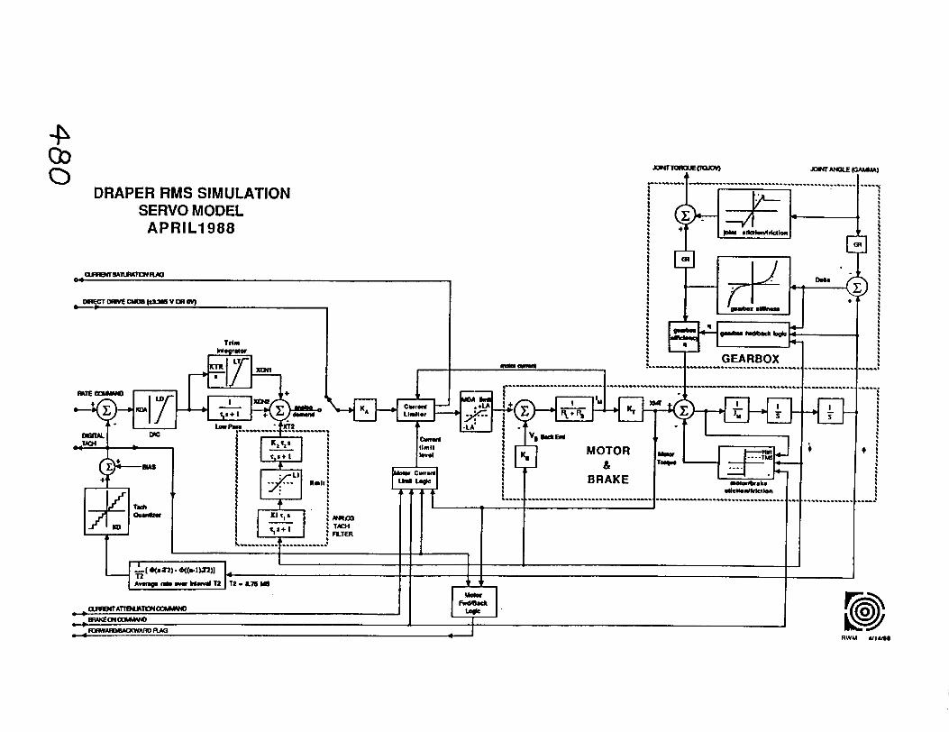


Simulation to Flight Overplot Cross-axis Bending Excited by PRCS Jet Firing
8000 lb PFTA Grappled by RMS

Simulation to Flight Overplot
In-plane Bending Excited by PRCS Jet Firing 8000 lb PFTA Grappled by RMS
- FLIOHT X ORS
TIME (SECI c. 3. ~ W L R w

Simulation to Flight Overplot Joint Angle & Motor Rate for
Shoulder Pitch Single Mode Drive 8000 lb PFTA Grappled by RMS
ENCODER ANGLE SHOULDER PITCH
0 ORS + FLIGHT
0.0 10.0 a0.0 30.0 co.0 sj.0 d . 0 TIHE 1SECOH)SI . 0 . s . m -
TRCHOMETER R A T E SHOULDER P ITCH

Simulation to Flight Overplot Motor Rate Start and Stop Transients for
Shoulder Pitch Single Mode Drive 8000 lb PFTA Grappled by RMS
.TACHOMETER RRTE SHOULDER PITCH
0 ORS FLIGHT
TRCHOMETER RRTE SHOULOER P ITCH


Simulation Applications of the DRS (cont)
FCS interaction
Stability analyses - Self sustaining limit cycles are possible -because of the relative values of FCS bandwidth, phase lag and fundamental bending frequency
Estimation of accelerations at the arm to payload interface due to PRCS jet activity
- JFT 7/12/88

FCS Stability Analyses
Stability is dependent on payload position and attitude relative to the Orbiter
For a candidate position and attitude:
.Apply open-loop PRCS pulses to excite the funamental flex modes of the system and then activate the FCS closed loop attitude hold, o r . Simulate three axis attitude maneuvers,
= Observe whether a self-sustained limit cycle results.
JFT 7 /12/88
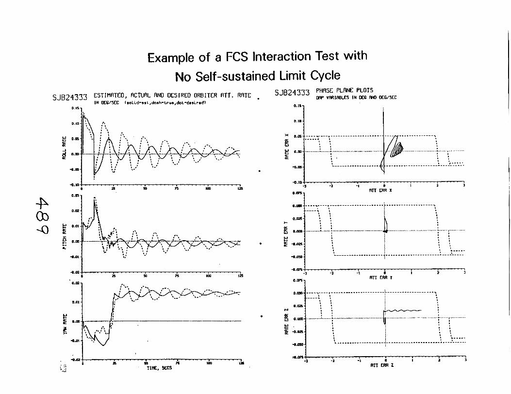
Example of a FCS Interaction Test with
No Self-sustained Limit Cycle cj ~ ~ 2 4 3 3 3 EST1 HATED, ACTUAL AND DESIRED ORBITER ATT . RATE
IN DE6/5EC (solid-yst,&sh-true,do~-desired) 0.15,
~824333 PHASE PLANE PLOTS DRP VfIRlABLCS IN OE6 AH) OCG/SEC
AT1 ERR Y

Example of a FCS Interaction Test with
-0.10 -3 -2 -1 0 1
F m 2 3
0.017 RTT ERR X
A Self-sustained Limit Cycle ~ 0 ~ 5 0 $ 3 0 ESTIMRATD, ACTUAL AND DESIRE0 ORBITER ATT. RATE ~ 0~50$30 P H ~ L A N E PLOTS
IN LEG/S&C (eolid-eeL,dosh-trua,dot-desiredl ORP VRRIABLES I N DEG RM) MO/YC 0.15 -
0. I0 -
0.m- a (L W
g a.m......
= . :
I ,
3.m - " I
- m m N U1
. - - - - - ? 9 -----i---'----------------- - - - - - _ _ _ - - - _ _ _ _ _ 3 O ?
........ ..... ............................... , I
....... ............ I *
I ! .......I , I z
I I 2
- - - - - - - - - - - - - - - - -__*--- - - - - - - - ' ;-----.


Draper's LSAD Simulation
*All flexibility between the orbiter and the payload is lumped into six relative degrees of freedom. The a rm is assumed to be massless. LSAD state vector has dimension six.
A simplified algorithm ,is used to model the response of the joint servos. This algorithm can operate at an 80 ms time step as opposed to the 1ms DRS time step.
Fidelity in the low frequency modes has been retained.
Features have been added:
Ability to submit sets of position and attitude variation cases in a single batch,
.Ability to start a simulation with the a rm in an excited state.
Cost of an LSAD run is about a factor of 10 less than the cost of a DRS run.
JFT 7/12/88

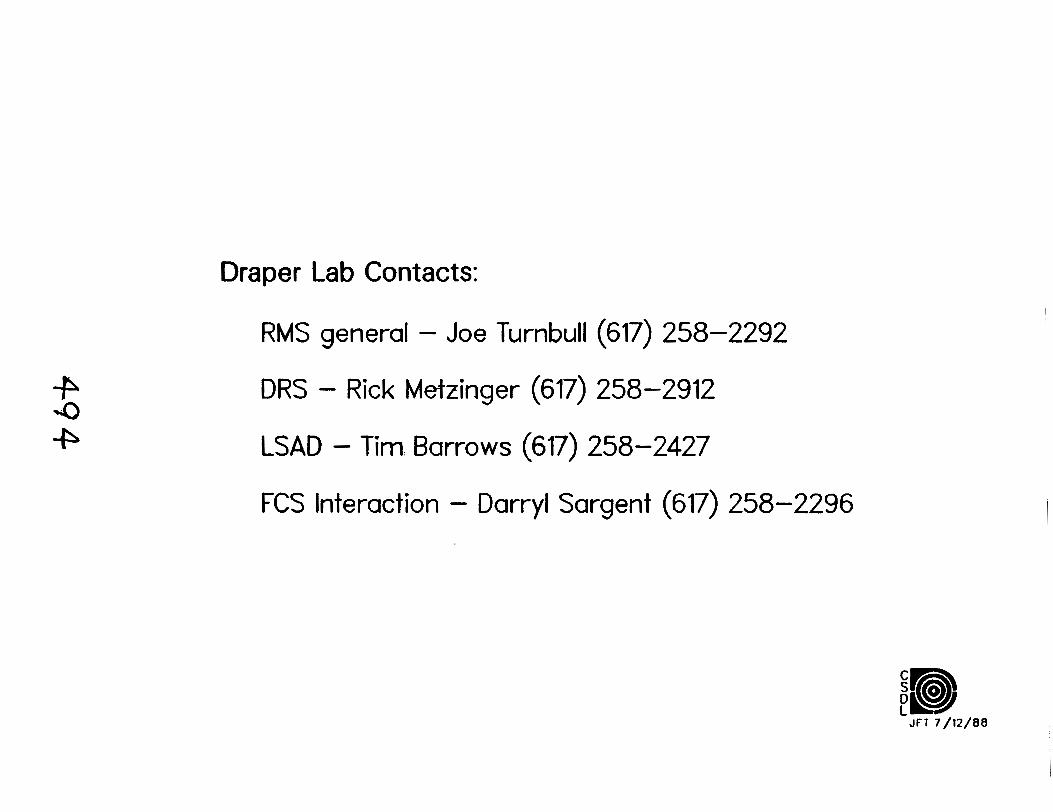
Draper Lab Contacts:
RMS general - Joe Turnbull (617) 258-2292
DRS - Rick Metzinger (617) 258-2912
LSAD - Tim. Barrows (617) 258-2427
FCS Interaction - Darryl Sargent (617) 258-2296
OR~GMAL FASE es OF WKR QUALITY
A PERFORMANCE COMPARISON OF INTEGRATION AULORITHMS IN SIMULATING FLEXIBLE STRUCTURES
R M. Howe The University of Michigan
Applied Dynamics International Ann Arbor. Michigan
ABSTRACT
Modeling of the dynamic vlbratlon modes of a flexible structure can be achieved either by uslng a generalized coordinate for each mode considered in the simulation, or by discretlzing the structure into a sufficiently large number of segments to provide the necessary modal accuracy. The accuracy and stability considerations in choosing appropriate numerical integration algorithms are dllrerent. depending on which modeling approach is utilized. In the generalized coordinate approach the frequency and shape of each mode is assumed to be known. The integratlon method should provide an accurate match to the modal frequency and damplng. and sh'ould also exhiblt sinusoidal transfer functlon errors whlch are acceptably small, especially for frequencies in the vicinity of the modal resonance. Since only those modes considered necessary for the required slmulation ndellty are included a s generalized coordinates. integrator stabillly for modes of higher frequency does not become in an issue.
On the other hand. when the dkcreiized structure approach is used, hfRh frequency modes not of interest to the simulation wlll nevertheless be present. In this case it is Important that the lntegratlon method not only provlde satisfactory characteristic root and transfer functlon accuracy for the lower modes of interest, but also provlde stable solutions with satisfactory damping for the higher modes which are not of interest.
~ ~ s y m p t o t i c formulas for the characteristic root errors a s well a s transfer functlon gainand phase errors are presented for a number of traditional integration methods and for several new lntegratlon methods. Normalized stablllty regions in the Ah plane are compared for the various methods. In particular. it is shown that a modined foml of Euler integration with root matching is an especially efficient method for slrnulatlng lightly-damped structural modes. The method has been used successfully for structural bending modes in the real-time simulation of missiles. Performance of this algorithm Is compared wlth other special algorithms. includlng the state-transition method. A predlctor-corrector version of the modifled Euler algorithm permlts it to be extended to the simulation of nonlinear models of the type likely to be obtained when using the dlscretlzd structure approach.
Performance of the different integration methods is also compared for integration step shes larger than those for whlch the asymptotic formulas are valid. It is concluded that many lradltional integratlon methods, such a s RD-4, are not competitive in the slmulation of llghtly damped structures.

.I * A Performance Comparison of Integration ~ l ~ o r i t h m ; in Simulating Flexible
Structures
R. M. Howe
The University of Michigan, Ann Arbor, Michigan
and
Applied Dynamics International, AM Arbor, Michigan
ABSTRACT
In this paper a number of integration algorithms, including several new methods, are considered for the simulation of flexible structures. The effectiveness of the different algorithms is assessed by considering the characteristic root errors which they produce, the sinusoidal transfer function gain and phase errors, the stability regions, and the execution times. The suitability of the various algorithms for simulations with real-time inputs is also noted. When the structural modes in a simulation are represented by generalized (normal) coordinates, the selection criteria for integration methods are somewhat different than the criteria when the structure is discretized into a sufficiently large number of segments to provide the necessary modal accuracy. In this paper asymptotic formulas for the characteristic root errors as well as transfer function gain and phase errors are presented for a number of traditional integration methods and for several new integration methods. Normalized stability regions in the hh plane are compared for the various methods. In particular, it is shown that a modified form of Euler integration with root matching is an especially efficient method for simulating structural modes. The method has been used successfully for structural bending modes in the real-time simulation of missiles. A predictor version of the modified Euler algorithm pennits it to be extended to the simulation of nonlinear models of the type likely to be obtained when using the discretized structure approach.
1. Introduction
Modeling of the dynamic vibration modes of a flexible structure can be achieved either by using a generalized coordinate for each mode considered in the simulation, or by discretizing the structure into a sufficiently large number of segments to provide the necessary modal accuracy. In this latter case the mathematical model for a flexible structure with N degrees of freedom has the following general form:
where q is an N-component position state vector, M(q) is the mass matrix, C(q,q) is the coriolis and centrifugal acceleration vector, K(q) is the elastic and gravity force vector, and F(t ) is the external force vector. When the vibration modes of the structure are represented by normal

(generalized) coordinates, a coordinate x representing the time-varying amplitude of a given mode with undamped natural frequency a+, and damping ratio [obeys the equation
H e n &t) is the generalized force associated with the coordinate x. When a number of modes are present, there will in general also be terms in Eq. (2) which couple the mode of amplitude x with other structural modes.
The accuracy and stability considerations in choosing appropriate numerical integration algorithms for solving differential equations of the type shown in (1) or (2) will be different. In the generalized coordinate approach of Eq. (2) the frequency and shape of each mode is assumed to be known. The integration method should provide an accurate match to the modal frequency and damping, and should also exhibit sinusoidal transfer function errors which are acceptably small, especially for frequencies in the vicinity of the modal resonance. Since only those modes considered necessary for the required simulation fidelity are included as generalized coordinates, integrator stability for higher frequency modes which are not of interest does not become an issue.
On the other hand, when the discretized structure approach represented by Eq. (1) is used, high frequency modes which are unimportant in the simulation will nevertheless be present. In this case it is important that the integration method not only provide satisfactory characteristic root and transfer function accuracy for the lower modes of interest, but also provide stable solutions with satisfactory damping for the higher modes which are not of interest.
In this paper asymptotic formulas for the characteristic root errors as well as transfer function gain and phase errors are presented for a number of traditional integration methods and for several new integration methods. Normalized stability regions in the Ah plane are compared for the various methods, where A is an eigenvalue asociated with the linearized perturbation equations of the structure and h is the integration step size. . In particular, it is shown that a modified form of Euler integration with root matching is an especially efficient method for simulating lightly-damped structural modes. The method has been used successfully for structural bending modes in the real-time simulation of missiles. Predictor versions of the modified Euler algorithm permit it to be extended to the simulation of nonlinear models of the type likely to be obtained when structures are represented by means of discretization. The stability regions in the Ah plane for the modified Euler methods are especially well suited to the requirements when using the discretized structure approach.
2. Dynamic Error Measures for Integration Algorithms
In comparing different integration methods for the simulation of flexible structures it is important to utilize meaningful performance measures which permit general conclusions to be drawn regarding the expected dynamic errors associated with each method. Our dynamic error analysis will be based on linearized perturbation equations derived from the original nonlinear differential equations used to model the structure. Thus we will assume that the system

eigenvalues ate known, as well as the transfer functions relating specific input-output pairs. We will further assume that the simulation uses a fixed integration step size h. This is necessary in the case of a real-time simulation. It is likely to be true over a large number of steps even when a variable-step integration method is used in simulating a flexible structure. For linearized equations and a fixed integration step size we can apply the method of z transforms to anayze the dynamic errors resulting from specific integration algorithms [1,2]. There are two error measures which quite useful in predicting overall dynamic accuracy in the simulation. The frst is the fractional error in each characteristic root (eigenvalue) of the digital simulation, defined as
a* - a Fractional error in characteristic root = eh = - A
where h is the characteristic root of the continuous system being simulated and A* is the equivalent characteristic root for the digital simulation. For the case of complex roots (of which there will be many conjugate pairs in the simulation of a flexible structure) it is more appropriate to determine the fractional error, ew, in root frequency and the damping ratio error, ey. Thus we define
Here 6): and ad represent the frequencies of the digital and continuous system roots, respectively, while c* and Crepresent the damping ratios for the digital and continuous system roots, respectively .
The second dynamic error measure of significance is the fractional error in digital system transfer function for sinusoidal inputs of frequency o. For any input-output pair let H(s) be the transfer function of the continuous system and H*(z) be the z transform of the digital system that results when a particular integration algorithm is used. Then the fractional error in sinusoidal transfer function is given by [3]
For simulations of any reasonable accuracy the magnitude of this fractional error will be small compared with unity, in which case it is easily shown that the real part, eM, is equal approximately to rfie fractional error in gain and the imaginary part, eA, is equal to the phase error of the transfer function [3].
For any numerical integration algorithm the integrator transfer function for sinusoidal inputs of frequency o can be written approximately as 131

where h is the integration step size. Since l l ( j ~ h ) is the ideal integrator transfer function, it is apparent that the term eI(joh).c represents the integrator error. For Adams-Bashforth predictor and Adams-Moulton two-pass predictor-corrector algorithms of order 2, 3, and 4, integration methods that are candidates for simulation of flexible structures, the error coefficient el and algorithm order k are listed in Table 1.
Table 1. Integrator Transfer Function Error Parameters for AB Predictor and AM Predictor Corrector Algorithms
Method Frror Coefficient, el m Or&, k
In terms of el and k the following formula for ea, the fractional error in characteristic root as defined earlier in Eq. (3). can be derived [3]:
It is apparent that ea is directly proportional to the integrator error coefficient, el. For complex characteristic roots equivalent asymptotic formulas for the root frequency and damping errors, ew and eG as &fined in Eq. (4), can be derived [3]. As in Eq. (7). the errors are proportional to e~ lUlk.
For digital simulation of a fist order system with transfer function H(s) = l/(s-A) the fractional error in the transfer function for sinusoidal inputs, as defined in Eq. (5). can also be derived in terms of the integrator error parameters el and k [3]. From this result the following asymptotic formulas are obtained for eM, the fractional error in transfer function gain, and eA, the transfer function phase error:

+ w2e, 9 w ~ e , Fork even, eM s - ( - I ) , (oh)k , eA z ( - 1 ) ( oh )k , wh cc 1 (9)
0 2 + n w2 + a2 Here the errors are proportional to el (oh)k. Comparable asymptotic formulas for eM and eA can be derived for digital simulation of a second-order system with transfer function H ( s ) = lI(s2 + 2Cw,s + o$) [3]. Again, the gain and phase errors are proportional to e,(oh)k.
The transfer function H(s) for any order linear system with both real and complex roots can be represented as the product of first and second-order transfer functions. In this case it can be shown that the asymptotic formulas for the digital system transfer function gain and phase errors is simply the sum of the individual first and second-order subsystem gain and phase errors, respectively, for predictor and predictor-corrector methods of the type shown in Table 1 . If we simulate a flexible structure with a given integration method, this permits us to compute the linearized system gain and phase errors at the frequency o for any input-output pair as a function of integration step size h. In view of the reemerging popularity of frequency-domain methods for designing multiple input/multiple output control systems, this is a quite useful result. It pennits us to estimate ahead of time for a given step size and integration method whether the simulation errors will be satisfactorily small. Conversely, for a given transfer function accuracy requirement, it allows us to compute the maximum allowable step size h for the simulation.
It should be noted that the methodology outlined above for determining characteristic root and transfer function errors for any order of linearized system from the simple integrator model given by Eq. (6) does not work in the case of multiple-pass, single step methods such as Runge-Kutta. This is because the results of individual passes within a single step in such methods depend on the particular form of the system transfer function. Asymptotic formulas for the root error parameters e2, eu and ey can, of course, be derived separately for RK-2, RK- 3, RK-4, and variations of these methods [3].
3. Modified Euler Integration Algorithms
In this section we describe some modifications of simple Euler integration which have potentid advantages over conventional integration methods such as those listed in Table 1. First we introduce the concept of state variables defined at both integer and half integer sample times. Assume that the simulation of a mechanical degree of freedom with position state x, velocity state y, and acceleration a involves integrating the following simple state equations:

Next assume that successive data points are defined at integer time samples in representing the acceleration a and position x, and at half-integer sample times in representing the velocity y. The following modified Euler algorithms can then be used for integration:
The basic concept behind this m&ication of standard Euler integration is very simple; instead of the using the state variable derivative defined at the beginning of the integration step, the method uses a state variable derivative defined halfway through the step. For this algorithm it is easy to show that the integrator error coefficient defined in Eq. (6) is given by el = 1/24 and the order of the method is k = 2. Thus the accuracy of this single-pass algorithm is twice that of the two-pass AM-2 predictor-corrector. However, the algorithm does require that the velocity states be defined at half-integer sample times.
Let us apply this modified Euler method to the second-order system represented by Eq. (2) for the generalized coordinate x. We can replace Eq. (2) by the following two state equations:
By analogy with Eq. (1 1) the modified Euler difference equations become:
Since yn is not explicitly computed, it is necessary to substitute an estimate y; in the damping term on the right side of the yn+ln equation. There are many ways in which they; estimate can be computed In Table 2 we list four candidate methods.
Table 2. Methods for Estimating the Velocity y, in Modified Euler Integration
Method for the Est ima, yj,
2. Extrapolation using yn- and yn -YZ
3. Integration using yn., and yn-2
4. Estimate based on yn- I
Yn=Yn-vz

The estimate for y, in the first method is simply based on averaging Yn+ln and This is equivalent to utiliiing trapezoidal integration for the damping term. Although this means that y,+,n now appears on both sides of the difference equation in (13), for the linear system considered here it is possible to solve explicitly for yn+ln, as we will see in the next section. In the second method the estimate for y, is based on a linear extrapolation from y,-ln and Yn-sn. This is equivalent to using trapezoidal integration for the damping term. Since yn+112 now appears only on the left side of the difference equation in (13), this method can be used in the simulation of equations where dyldt is a nonlinear function of y. This is also true for the third and fourth methods. The third is based on a second-order predictor integration over the interval h/2, starting with yn.l12 and using dyldt at the n-1 and n-2 intervals. This is equivalent to estimating y, with quadratic extrapolation based on yn.i/z, yn-312 and Yn-sn. In the fourth method we simply use Yn-ln as our estimate for y,. This is equivalent to Euler integration for the damping term.
4. Modified Euler Integration with Trapezoidal Damping
We have seen in Table 2 that the velocity estimate yh for the modified Euler difference equations in (13) can be based on the average of yn+lD and Yn-ln. Thus
As noted earlier, this is equivalent to utilizing trapezoidal integration for the damping term. Although this means that yn+ln now appears on both sides of the difference equation, for the linear system considered here it is possible to solve explicitly for y,+ln. In this way we obtain the following equations:
where
From the method of z transforms applied to Eqs. (15) and (16) we obtain the following asymptotic formulas for the frequency and damping ratio errors of the digital simulation 141:
The transfer function gain and phase errors are given approximately by

Fractional - w*l --- - gain cmr 1~ l = e M = (Oh), Oh<< 1
The characteristic root errors in Eq. (17) and the transfer function gain and phase errors in Eqs. (18) and (19) art comparable with those for AM-2 integration for the same step size h [3]. Yet AM-2 is a two-pass method whereas the modified Euler with trapezoidal damping, as used here, is a single-pass method. Thus it will take only half as long to execute as AM-2 while producing comparable accuracy. Its accuracy is approximately 5 times better than the accuracy of AB-2 integration when applied to the same second-order system.
Tht accuracy of modified Euler integration when applied to a linear second-order system can be further improved by the technique of root matching, which was originally employed by Fowler to improve the performance of conventional Euler integration [5]. By taking the z transform of Eqs. (15) and (16) we can obtain exact analytic formulas for the undamped natural frequency cq,* and damping ratio C[* in terms of On and C. From these formulas we can solve for a and C in terms of oh* and p. If in these formulas we then replace cq, and C by on' and C, respectively, and q,* and C* by On and C, respectively, we obtain the following [4]:
If on' and from these formulas are used instead of on and in Eqs. (15) and (16), the resulting digital simulation will exhibit q,* and C* values which exactly match the w, and C[of the continuous system being simulated. For a given step size h the on', c, C1 and C2 can be precomputed, so that each integration step in simulating the second-order system only requires 3 multiplies and 2 adds, as before. Now the charcteristic roots of the digital simulation will be exactly equal to those of the continuous system, regardless of the integration step size h. The approximate formulas for the transfer function gain and phase errors are given by [4]:

Note that the fractional error in gain, eM, is completely independent of the damping ratio c, and the phase error eA approaches zero as C approaches zero. Thus our modified Euler algorithm with root matching will be especially effective in simulating lightly-damped second-order systems, as will be the case in structural modes. This is illustrated in Figure 1, where gain and phase versus frequency for a second-order system with C = 0.01 are plotted. Because of the sharp resonant peak in gain and the extremely rapid change in phase as u passes through on, it is very critical that both the natural frequency and damping ratio of the digital simulation match that of the continuous system. The table at the bottom of the figure shows the transfer function errors for input frequencies in the vicinity of an for the specific case of onh = 0.5, which corresponds to only 2 integration steps per radian or 12.57 steps per cycle. Shown in the table are the gain and phase errors based on both an exact calculation from the system z transform, H*(dd), as well as the approximate formulas of Eq. (31). Note how closely the approximate caculations agree with the exact, even for the example here for which wh = 0.5.
Until now we have only analyzed the dynamic performance of the modified Euler method in the frequency domain. This has been accomplished by examining the gain and phase errors of the transfer function for sinusoidal inputswe now consider the errors in computed response of the second-order system to a unit-step input. Figure 2 shows the errors which result when using RK-2 integration (Heun's method); modified Euler with trapezoidal integration for the damping term, i.e., Eqs. (15) and (16); and modified Euler with root matching, i-e., a+,' and from Eqs. (20) and (21) substituted for a+, and in Eqs. (15) and (16). For the example in the figure the damping ratio t = 0.707 and the integration step size is given by o,h = 0.5. The results show that the RK-2 errors are 4 to 10 times larger than the modified Euler errors. It should also be noted that RK-2 is a two-pass method, that is, it requires two evaluations of the state-variable derivatives per integration step. It follows that RK-2 will take approximately twice as long to execute per integration step as the single-pass modified Euler methods. To provide the same output integration frame rate in real time the RK-2 method will therefore require twice the mathematical step size h in comparison with the modified Euler methods considered here. This will further increase by a factor of 4 the RK-2 errors relative to the modified Euler errors in Figure 2.
The modified Euler results shown in Figure 2 were obtained using an initial step of W2 in integrating dydt to obtain y. After one integration step this provides the calculation of y l n starting with the initial condition yo. The step size is taken as h for all subsequent dyjdr integration steps. This results in successive velocity values representing y at half-integer step times, consistant with the concept introduced in the beginning of this section.

Fractional Gain Error Phase Error (radians)
do, Exact Eq. (3 1) Exact Eq. (3 1)
onh = 0.5 0.7 0.01040 0.01021 -0.000296 -0.000292 0.9 0.01727 0.01888 -0.000381 -0.000375
12.57 steps 1 .O 0.021 37 0.02083 -0.000424 -0.0003 17 per cycle) 1.1 0.02592 0.02521 -0.000467 -0.00045 8
1.4 0.04240 0.04083 -0.000595 -0.000583
Figure 1. Frequency response of lightly-damped second-order system using modified Euler integration with root matching, o ,h = 0.5.

m I RK-2 I 0.03 0 Modified Euler
Error 4 Modified Euler
Figure 2. Unit step response errors in simulating a second-order system with damping ratio C = 0.707, integration step size given by a h = 0.5.
5. Performance of Other Versions of Modified Euler Integration
In this section we present the asymptotic formulas for characteristic root and transfer function emrs when modified Euler integration is used to simulate a second-order system with methods 2, 3, or 4 in Table 2 utilized to calculate the velocity estimate yh in Eq. (13). For method 2, which is equivalent to AB-2 integration for the damping term, the following results are obtained for em the fractional error in root frequency, and eG the damping ratio error 161:
These errors are significantly less than the errors when AB-2 is used for all integrations. For method 3 in Table 2, which uses a second-order predictor integration algorithm to compute y;, the following asymptotic formulas are obtained for the root frequency and damping errors:
The transfer function gain and phase errors are given by

In both Eqs. (24) and (25) the errors are a factor of two smaller than the comsponding errors when AM-2 is used for all integrations. In addition, the AM-2 algorithm is a two-pass method which will therefore take twice as long to execute on a given computer. For method 4 in Table 2, which is equivalent to using Euler integration for the damping term, the following formulas are obtained for the characteristic root and transfer function e m [4]:
Note that the errors are all proportional to the first power of the step size h. This is because of the first-order Euler algorithm used for integration of the damping term. For 5. = 0, however, the first-order errors in Eqs. 25) and (26) vanish, meaning that the errors become second-order in h. This is to be expected, since the conventional Euler integration plays no role when C = 0. In fact it can be shown that when c= 0, the digital solution will have zero damping regardless of the step size h.
When method 2,3, or 4 in Table 1 (or any other explicit method) is used to provide the estimate yh for the velocity state, the modified Euler method can be used as the algorithm for integrating the nonlinear state equations represented by (1). The vector difference equations become the following:
We now turn to a consideration of integration algorithm stability.

6. Stability of Integration Methods
It has already been pointed out that the stability of numerical integration algorithms becomes an important consideration when the flexible structure is modeled by discretization. This is because the dismtized model will contain high frequency modes which arc unimportant in the simulation but can cause numerical instabilities for reasonable integration step sizes. For a given integration method the stability boundary in the Ah plane can be obtained by considering a simulation of the linear system with transfer function H(s) = l/(s-A). From the difference equation the z transform, H*(z), is obtained. The stability boundary is defined by the Ah values for which the denominator of H*(z) vanishes when Izl = 1. These Ah values can be obtained by letting z = doin the denominator of H*(z) and solving for Ah for 8 values ranging between 0 and n. When this is done for the AB predictor methods, the stability regions plotted in Figure 3 an obtained. The regions are symmetric with respect to the rtal axis so that only the upper half plane is shown. For any values of Ah lying outside the boundaries the digital simulation will be unstable. In the case of both AB-3 and AB-4 the boundary crosses over into the right half plane. This means that a continuous system with roots on the imaginary axis which correspond to undamped transients can exhibit stable transients in the digital solution. Put another way, it means that AB-3 and AB-4 solutions will exhibit more damping than the continuous system being simulated. This is actually desirable in the case of the high frequency modes which are not of interest in a given simulation. On the other hand the AB predictor methods do not have particularly large stability regions and therefore do not permit very large integration step sizes h compared with the reciprocal magnitude, 1/12, of the largtst eigenvalues in the simulation.
Figure 3. Stability boundaries for AB predictor integration.
In Figure 4 the stability boundaries are shown for the the two-pass AM predictor-corrector methods. Although the boundaries are considerably larger than those for the AB methods, it must be remembered that the AM algorithms will take twice as long to execute. Thus the boundaries should be reduced by a factor of two for a valid comparison with AB-2. When this

is done, the AM-2 and 3 boundaries actually fall inside the AB-2 and 3 boundaries, dthough me AM-4 boundary still Lies outside the AB-4 boundary. In all cases the higher-order algorithms exhibit less stability end are thexeforc unlikely to k candidates for simulating flexible s-s.
Figure 4. Stability boundaries for two-pass AM predictor-corrector integration.
For comparison purposes the stability boundaries for RK-2, 3 and 4 are shown in Figure 5. We recall that these algorithms require 2, 3 and 4 passes, respectively, through the state equations per integration step. Thus for proper comparison with single-pass methods the boundaries shown should be reduced by factors of 2.3 and 4, respectively. When this is done. the RK-2 boundary roughly matches the AB-2 boundary, while the RK-3 and RK-4 boundaries still fall outside the AB-3 and 4 boundaries, respectively.
-3 -2 -1 0 +1
Figure 5. Stability boundaries for Runge-Kutta integration methods.

Finally, in F i g ~ 6 arc shown the stability boundaries far various modifled Euler mthods, as described in Sections 4 and 5. The trapezoidal damping case Consponds method 1 in Table 2, the Euler damping case to method 4, the AB-2 damping case to method 2, and the predictor damping case to method 3. Also shown for comparison purposes in figurc 6 are the stability boundaries for AB-2, AM-2 and RK-2, as presented earlier in Figuns 3,4 and 5, respectively. The AM-2 and RK-2 stability boundaries have been reduced by a factor of two to reflect the two passes per integration step required in the implementation of these metho&. Note that all four of the Modified Euler methods in Figure 6 have stability regions which pmnit values of I U l up to 2 for lightly damped transients, e.g., eigenvalues near the imaginary axis. In this regard the methods an considerably superior to the AB-2, AM-2 and RK-2 algorithms and should perform especially well in the simulation of flexible seucnncs.
It should also be noted that the modified Euler methods an ideally suited for real-time simulation in that they do not require inputs prior to their occurence in real time. For example, if F(t) in Eq. ( 1 ) is a real time input, then the single-pass modified Euler algorithm of Eq. (28) only requires Fn at the beginning of the nth integration step. On the other hand, the AM prcdictorcomctor algorithms require F H 1 at the start of the second pass for the nth integratim step, and F,,+l is not yet available in real time. Then is, however, a modified version of the AM-2 predictor method which is compatible with real-time inputs [6]. The AB predictor methods are also compatible with real time inputs, and there are versions of RK-2 and RK-3 which permit real-time inputs [3]. RK-4 is not compatible with real-time inputs, since it rtquires Fn+1n at the beginning of the seco~~d pass and Fn+l at the start of the fourth pass, in both cases prior to their availability in real time.
j l . 0
Figure 6. Stability boundaries for modified Euler integration methods.

7. Conclusions
In this paper we have considered the dynamic performance of integration methods in the context of simulating flexible structures. In terms of both characteristic root errors and transfer function errors, both important in such simulations, we have compared the performance of traditional integration methods with various versions of modified Euler integration . We have shown that modified Euler integration is especially effective in simulating lightly-damped structural modes. We have also shown that the modified Euler methods have very favorable stabilty boundaries in the Ah plane with respect to requirements in the simulation of lightly- damped modes. This is especially significant when a flexible structure is modeled by discretization as opposed to normal coordinates, since it will allow larger integration step sizes before the solution goes unstable due to the presence of higher modes which are unimportant to the simulation.
References
1. Gilbert, E.G., "Dynamic Error Analysis of Digital and Combined Digital-Analog Systems," Simulation, vol. 6, no. 4, April 1966, pp 241-257.
2. Benyon, P.K., "A Review of Numerical Methods for Digital Simulation," Simulation, vol. 1 1, no. 4, Nov. 1968.
3. Howe, R.M., "Transfer Function and Characteristic Root Errors for Fixed-Step Integration Algorithms," Transactions of the Society for Computer Simulation, vol. 2, no. 4, Dec. 1985, pp 293-320.
4. Howe, R.M., "Simulation of Linear Systems Using Modified Euler Integration Methods," to appear in Tranractioru of the Society for Computer Simulation.
5 . Fowler, M.E., "A New Numerical Method for Simulation," Simulation, vol. 4, no. 5, May 1965, pp 324-330.
6. Howe, R.M., "The Role of Modified Euler Integration in Real-Time Simulation," Proceedings of the Conference on Aerospace Simulation II , San Diego, 1986; pp 263-275. The Society for Computer Simulation, P.O. Box 17900, San Diego, CA 921 17.

THIS PAGE INTENTIONALLY LEFT BLANK

OPTICAL PROCESSING FOR DISTRIBUTED SENSORS IN CONTROL OF FLEXIBLE SPACECRAFT
NASA LANGLEY RESEARCH CENTER SPACECRAFT CONTROL BRANCH
HAMPTON, VA 23665-5225

OPTIC= PROCESSING FOR DISTRIBUTH) SENSORS I N CONTROL OF FLEXIBLE SPACECRAFI'
Raymond C . Montgomery, Sharon S. Welch Michael F. Barsky, and I a n T. G a l l i m r e
NASA Langley Research Cen te r Hampton, VA 23665-5225
i
ABSTRACT
'rhia-psee*a&L~~--- a r e c e n t p o t e n t i a l of d i s t r i b u t e d image p r o c e s s i n g / Appl ica t ions i n t h e cont r%l of f l e x i b l e s p a c e c r a f t wi-Ef be ' . ' emphasized. Devices a r e c u r r e n t l y be ing developed a t NASA and i n u n i v e r s i t i e s and i n d u s t r i e s t h a t a l l ow t h e r ea l - t ime process ing of holographic images. With in 5 y e a r s , it is expected t h a t , i n rea l - t ime, one may add o r s u b t r a c t ho log raph ic images a t o p t i c a l accuracy . Images a r e s t o r e d and processed i n c r y s t a l mediums. The accuracy of t h e i r s t o r a g e and p rocess ing is d i c t a t e d by t h e g r a t i n g l e v e l of l a s e r holograms. ~t is f a r g r e a t e r t h a n t h a t ach ievab le u s i n g c u r r e n t ana log - to -d ig i t a l , pixel o r i e n t e d , image d i g i t i z i n g and canpu t ing techniques .
P rocesso r s us ing image p r o c e s s i n g a l g e b r a can concep tua l ly be des igned t o mechanize F o u r i e r t ransforms, l e a s t square latt ice f i l t e r s , and o t h e r complex c o n t r 01 system ope ra t ions . Thus, a c t u a t o r command i n p u t s de r ived f r a n conplex c o n t r o l l a w s i nvo lv ing d i s t r i b u t e d holographic images can be genera ted by such a n image p rocesso r . T w - m a l p l ans f o r t h e development of a Conjugate O p t i c s Processor f o r c o n t r o l of a f l e x i b l e o b j e c t .
/ C t
, f s * P


PRESENTATION OUTLINE
Th i s t a l k d e a l s wi th p l a n s t o develop o p t i c a l d i s t r i b u t e d s e n s o r s and c a n p u t a t i o n t echn iques f o r t h e c o n t r o l of f l e x i b l e s t r u c t u r e s . The p l a n i s t o develop t h e technology r e l a t i v e t o a c t i v e v i b r a t i o n damping of s t r u c t u r a l dynamics sys tems and, t hen , t o demonst ra te it w i t h a closed-loop c o n t r o l system experiment i n t h e l a b o r a t o r y . F i r s t , o b j e c t i v e s of t h e r e s e a r c h w i l l b e p r e s e n t e d . Next, fundamentals of o p t i c a l canputing w i l l be b r i e f l y over- viewed and new c a p a b i l i t i e s i n r ea l - t ime holography and holographic informa- t i o n s t o r a g e w i l l be d i scussed . An experiment being developed a t Langley w i l l be p r e s e n t e d wi th emphasis on t h e senso r concept and t h e o p e r a t i o n s unique t o o p t i c a l d i s t r i b u t e d process ing . The t a l k concludes w i t h a s t a t u s summary of both t h e a n a l y t i c a l and l a b o r a t o r y work i n t h i s a r ea .

OBJECTIVES OF RESEARCH
CONTROL OF FLEXIBLE STRUCTURES
DEVELOP DISTRIBUTED SENSORS DEVELOP DISTRIBUTED COMPUTATION TECHNIQUES USE NEW TECHNOLOGY FOR OPTICAL PROCESSING

OBJECTIVES OF RESEARCH
Object ives of t h i s research c e n t e r around t h e i n t e r e s t i n a c t i v e c o n t r o l of f l e x i b l e spacecra f t s t r u c t u r e s . The i n t e n t i o n is t o develop d i s t r i b u t e d sensors f o r t h i s app l i ca t ion and complimentary d i s t r i b u t e d cauputing tech- n iques . This has been enabled by recen t advances i n rea l - t ime holography using pho to re f rac t ive c r y s t a l s . Hence, some research o b j e c t i v e s w i l l be d i r e c t e d t o laboratory development of o p t i c a l processing using t h e new rea l - t ime holography techniques.


ADVANTAGES OF OPTICAL COMPUTING
Here we list some advantages of optical canputing. Paral le l mult ipl icat ion and addition are possible via optical canputing but, more importantly, the potential of distributed sensing and s ignal processing e x i s t s .
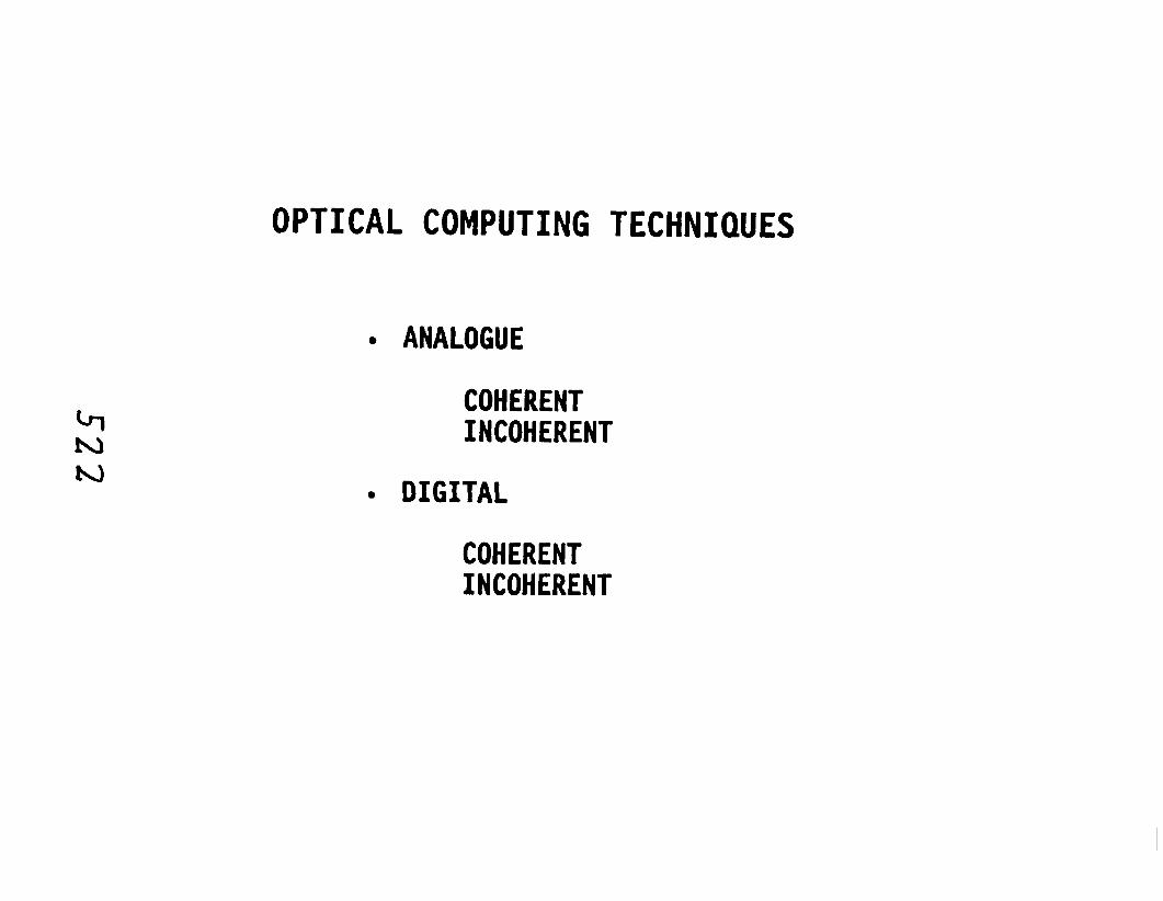

OPTICAL COMPUTING TE(NN IQUES
Both analogue and dig i ta l computing are possible via optics . These can be accanplished via both coherent a d inccherent l i gh t . Our work w i l l , however, be directed at analogue and coherent processing.

COHERENT ANALOGUE OPTICAL COMPUTING Plane wave
Fourier transform
Output image
plane
\
Input Input Output image mask image uperal
g H g*h convolution g H* gob correlation

COHERENT ANALOGUE OPTICAL COMPUTING
An example of a coherent ana logue o p t i c a l p rocesso r , a p l ane wave c o r r e l a t o r , i s i l l u s t r a t e d i n t h i s s l i d e . The p l a n e wave c o r r e l a t o r performs two-dimensional c o r r e l a t i o n o r convo lu t ion ope ra t ions on two i n p u t f u n c t i o n s g ( x , y ) , and h ( x , y ) . The o p e r a t i o n s of c o r r e l a t i o n and convolu t ion a r e performed i n t h e fo l lowing way. An image t r anspa rency (mask) with t r ansmi t - t a n c e g ( x ,y ) , shown h e r e a s a n image of t h e l e t t e r "T", is placed i n t h e f r o n t f o c a l p l a n e of l e n s L1 ( I n p u t Image P l a n e ) . An u n d i s t o r t e d p l ane wave of cohe ren t l i g h t i s passed through t h e image mask which in t roduces phase and ampl i tude changes i n t h e l i g h t . I n t h e back f o c a l p l ane of l e n s L1 t h e l i g h t ampl i tude d i s t r i b u t i o n is p r o p o r t i o n a l t o t h e F o u r i e r Transform of t h e trans- m i t t a n c e of t h e inpu t mask, g ( x , y ) . Thus, t h e back f o c a l p l a n e of L1, t h e F o u r i e r Trans form Plane , has c o o r d i n a t e s which coorespond t o spatial frequen- c i e s , h e r e denoted by k and k . I f a second mask is i n s e r t e d i n t h e
X Y F o u r i e r Transform Plane with t r a n s m i t t a n c e H(kx,k ) , t h e n t h e l i g h t propagated
Y through t h i s mask i s GH, where G is t h e Four ier t ransform of g. The second lens L2 per forms a F o u r i e r t r ans fo rm of t h e product G H , and thus , t h e image which i s formed i n t h e Output Image Plane i s t h e i n t e n s i t y of t h e convo lu t ion of g w i t h h , where h is t h e i n v e r s e F o u r i e r t ransform of t h e second mask H. S i m i l a r l y , i f t h e mask i n s e r t e d i n t h e Four i e r t ransform p lane i s H*, t h e image formed i n t h e Output Image P l a n e i s t h e c o r r e l a t i o n of g w i t h h.
I n t h e example shown i n t h i s s l i d e , t h e input f u n c t i o n i s a n image of t h e letter "T", and H(kx,k ) is a c i r c u l a r ape ra tu re . The image formed i n t h e
Y Output Image Plane is t h e convo lu t ion of t h e image "T" with t h e i n v e r s e F o u r i e r t r a n s form of t h e c i r c u l a r a p e r a t u r e func t ion H( k ,ky) . The image
X
which appears i n t h e Output Image P l a n e i s a n image of t h e l e t t e r "T" w i t h t h e h igh s p a t i a l f r equenc ie s removed.
Although a simple f u n c t i o n was used i n t h i s example f o r H, i n gene ra l t h e mask o r f i l t e r may be canplex and c o n t a i n both ampli tude and phase va r i a - t i o n s . To c o n s t r u c t a mask ( f i l t e r ) which c o n t a i n s both ampl i tude and phase i n f o r m a t i o n , i n t e r f e r a n e t r i c t echn iques a r e used. The mask t h u s formed i s a ho log raph ic f i l t e r .

CONSTRUCTION OF A HOLOGRAPHIC FILTER Coherent
Recording media
4- Interference pattern

CONSTRUCTION OF A HOLOGRAPHIC Ff LTER
Now consider t h e cons t ruc t ion of a holographic f i l t e r (mask). A holographic f i l t e r ( o r hologram) is simply t h e recorded in te rmi ty d i s t r i b u t i o n corresponding t o t h e i n t e r f e r e n c e of two ( o r more) l i g h t waves. The b a s i c geometry f o r const ruct ing a hologram of a t h r e e dimensional d i f f u s e l y r e f l e c t i n g o b j e c t is shown i n t h i s s l i d e . An i n c i d e n t coherent plane wave is divided i n t o two p lane waves. One, t h e reference beam, t r a v e l s d i r e c t l y toward t h e recording media ( A ) . The second, t r a v e l s toward t h e ob jec t . The p o r t i o n of t h e wave r e f l e c t e d f r a n t h e ob jec t (B) i s charrged i n both amplitude and phase. This r e f l e c t e d o b j e c t beam i n t e r f e r e s with t h e reference beam a t t h e p l a n e of t h e recording media. The recotding media ( u s u a l l y f i l m ) records t h e l i g h t i n t e n s i t y d i s t r i b u t i o n of t h e i n t e r f e r e n c e of A with B.
The i n t e r f e r e n c e pa t t e rn need not be const ructed as described above, bu t may be generated a r t i f i c i a l l y using a canputer . Canputer generatad holograms can be recorded on f i lm o r on a s p a t i a l l i g h t modulator. The recorded hologram p r w i d e s a means of nwdulatirq ( i .e . , f i l t e r i n g ) a l i g h t beam.


HOLOGRAPHIC FILTER TRANSMITTANCE
I n t h i s s l i d e is t h e mathematical expression which desc r ibes t h e l i g h t i n t e m i t y d i s t r i b u t i o n a t t h e recording media (previous s l i d e ) . The expres- s i o n f o r t h e i n t e n s i t y I ( x , y ) is composed of t h r e e terms. The f i r s t two terms a r e p ropor t iona l to t h e i n t e n s i t i e s of t h e reference wave and object wave r e s p e c t i v e l y . The t h i r d term is t h e i n t e r f e r e n c e term and depends upon t h e r e l a t i v e phases of the reference and ob jec t beams.
The seconi expression i s t h e t ransmit tance of t h e developed fi lm. The f i r s t term i n t h i s expression is a constant which r e s u l t s from uniform
2 exposure over t h e recording media, t h a t is, t h e A term i n t h e expression f o r t h e i n t e n s i t y . The remaining t h r e e terms a r e , r espec t ive ly , t h e in terrs i ty of t h e o b j e c t beam, t h e product of t h e complex conjugate of t h e f i e l d amplitude of t h e re fe rence and t h e f i e l d amplitude of t h e ob jec t and t h e product of t h e f i e l d amplitude of t h e reference and t h e complex conjugate of t h e o b j e c t .
When t h e recorded hologram is i l luminated with a beam which is t h e exac t d u p l i c a t e o f the reference wave, t h e f i l t e r r econs t ruc t s t h e o r i g i n a l ob jec t wave, B. I f t h e hologram is i l lumina ted with a beam which is t h e conjugate of t h e re fe rence wave, the f i l t e r r e c o n s t r u c t s the conjugate of t h e ob jec t beam, o r B*.

REAL-TIME HOLOGRAPHY WITH A VARIABLE MASK
REQUIRED FOR MANY OPTICAL COMPUTING APPLICATIONS
TWO TECHNIQUES AVAILABLE
cl-r - S P A T I A L L I G H T MODULATORS Crr) 0 - DFWM I N PHOTOREFRACTIVE CRYSTALS

REAL-TIME HOLOGRAPHY WITH A VARIABLE MASK
For many o p t i c a l processing a p p l i c a t i o n s it is necessary t o change o r update t h e holographic f i l t e r rea l - t ime. Two methods e x i s t f o r recording a holographic f i l t e r real- t ime, us ing devices known a s s p a t i a l l i g h t modulators, o r using a nonl inear o p t i c a l technique known a s degenerate four wave mixing (DFWM) i n a pho to re f rac t ive c r y s t a l .
A s p a t i a l l i g h t modulator i s a device composed of a matrix of i n d i v i d u a l p i x e l s of va r i ab le o p t i c a l t r a m m i t t a n c e . The t r ansmi t t ance of an ind iv idua l p i x e l is ad jus ted by varying a vo l t age t o t h e p ixe l . The p i x e l vo l t ages a r e addressable i n x and y. One example of a s p a t i d . l i g h t modulator i s a l i q u i d c r y s t a l d i sp lay .

SPATIAL L IGHT MODULATORS
ADVANTAGES
PROVEN TECHNOLOGY
INTERFACE WITH DIGITAL SYSTEMS
DISADVANTAGES
LOW RESOLUTION

SPATIAL LIGHT MODULATORS
Advantages of spat ia l l i g h t modulators is that they are a proven technology. They can a l s o be driven conveniently with s i g n a l s fram d i g i t a l computers. Also, the ir outputs can be conveniently interfaced v ia photodiodes t o d i g i t a l canputers.
The disadvantages of these devices is that they have r e l a t i v e l y low s p a t i a l reso lut ion .

DFWM I N PHOTOREFRACTIVE CRYSTALS
ADVANTAGES
HIGH RESOLUTION
ALL OPTICAL
SIGNAL AMPLIFICATION POSSIBLE
DISADVANTAGES
DIFFICULT TO WORK WITH (MANY VARIABLES)

DFWM I N PHOTOREFRACTIVE CRYSTALS
Advantages of DFWM are: extremely high s p a t i a l resolut ion ( a t t he l eve l of atomic p a r t i c l e s ) , a l l op t i ca l systems, and the po ten t ia l f o r op t i ca l s i gna l amplification. Signal amplif icat ion is perhaps one of t he most impor- t a n t advantages. Typically, i n an op t i ca l system about 4% of t he l i g h t i s l o s t a s the beam passes through each opt ica l element due t o sca t te r ing , i n t e rna l r e f l ec t i ons , and so on. This can be reduced somewhat with op t i ca l coatings, but even with op t i ca l coatings some l i g h t is l o s t . The r e s u l t is t h a t t h e l i g h t beam w i l l be s i g n i f i c a n t l y attenuated a f t e r passing through a r e l a t i v e l y few number of components ( i . e . , lenses, masks, e t c . ). With DFWM, s igna l amplification on the order of 1 0 0 is possible , and thus, the problem of s igna l a t tenuat ion can be overcome.
The grea tes t disadvantage of DFWM is tha t the devices a r e s t i l l i n t h e development stage. There a r e many var iables such a s beam alignment, tempera- t u r e , l i g h t in tens i ty , e tc . t h a t must be careful ly adjusted, and a s a r e s u l t , t h i s t echniqw of doing real-time holography is d i f f i c u l t t o implement.

Write
Object
DFWM IN PHOTOREFRACTIVE MEDIA
C axis
r u Crystal (BSO, BaTi03, LiN03) Phase conjugate beam

DFWM I N PHOTOREFRACTIVE MEDIA
I n t h i s s l i d e is a diagram i l l u s t r a t i n g t h e t y p i c a l geometry f o r performing degenerate four wave mixing (DFWM) i n a p h o t o r e f r a c t i v e c r y s t a l . Some examples of pho to re f rac t ive c r y s t a l s a r e Bismuth S i l i c o n Oxide (BSO) , Barium T i t a n a t e (BaTiOj), and Li th ium Niobate (LiN03). DFWM is a non l inea r
o p t i c a l p rocess whereby a phase con juga te beam is produced by mixing ( o r causing t o i n t e r f e r e ) t h r e e coherent beams of l i g h t of t h e same wavelength w i t h i n a medium.
The medium i n t h i s case is a pho to re f rac t ive c r y s t a l . The p h o t o r e f r a c t i v e c r y s t a l provides a unique way of recording l i g h t i n t e n s i t y which a1 lows mul t ip le beams t o be mixed. Light i n c i d e n t upon a photorefrac- t i v e c r y s t a l causes trapped charges wi thin t h e c r y s t a l t o migrate. The charges migrate t o regions of low l i g h t i n t e n s i t y and becane re t rapped. I f t h e l i g h t i n t e n s i t y d i s t r i b u t i o n over t h e c r y s t a l i s no t uniform, then a non- uniform d i s t r i b u t i o n of charge w i l l be e s tab l i shed wi th in t h e c r y s t a l . This d i s t r i b u t i o n of charge w i l l i n t u r n give r i s e t o a s p a t i a l l y varying e l e c t r i c f i e l d . The induced e l e c t r i c f i e l d causes a change i n t h e index of r e f r a c t i o n through t h e e lec t ro -op t i c e f f e c t . I n t h i s way, t h e d i s t r i b u t i o n of l i g h t i n t e n s i t y wer t h e volume of t h e c r y s t a l is recorded a s a change i n index of r e f r a c t i o n .
I n t h e diagram, t h r e e coherent beams of l i g h t , t h e w r i t e beam, t h e o b j e c t beam, a rd t h e read beam a r e i n c i d e n t upon a pho to re f rac t ive c r y s t a l simultane- ously . The i n t e r f e r e n c e p a t t e r n generated by t h e i n t e r f e r e n c e of t h e s e t h r e e beams, produces ( a s described a b w e ) a s p a t i a l l y varying index of r e f r a c t i o n wi th in t h e c r y s t a l . The v a r i a t i o n i n index of r e f r a c t i o n wi thin t h e c r y s t a l i s s i m i l a r t o a recorded hologram, and causes d i f f r a c t i o n of t h e beams. I f t h e read beam is i d e n t i c a l t o t h e w r i t e beam and counterpropagat ing with r e s p e c t t o t h e w r i t e beam, t h e d i f f r a c t e d beam is t h e phase conjugate of t h e o b j e c t beam.
DFWM i n a pho to re f rac t ive c r y s t a l is s i m i l a r t o convent ional holography where t h e hologram is i l luminated wi th t h e phase conjugate of t h e re fe rence , producing a phase conjugate of t h e o b j e c t . The d i f fe rence between DFWM and convent ion& holography is t h a t i n t h e DFWM process, t h e hologram i s w r i t t e n and read simultaneously. Because of t h e f a s t response t imes of many photo- r e f r a c t i v e c r y s t a l s , holography may be performed real- t ime using DFWM i n a p h o t o r e f r a c t i v e c r y s t a l .

co TWO-CRYSTAL OSCILLATOR FOR STORAGE AND COMPUTING
Write beam Read beam 1 Object beam 1 --\ crystal
Object beam --/& Photorefractive Write beam 2 crystal Read beam 2
TWO-CRYSTAL OSCILLATOR FOR STORAGE AND COMPUTING
I l l u s t r a t e d i n t h i s s l i d e is a schematic diagram of a new o p t i c a l memory being developed a t NASA Langley. The memory w i l l a l low more e f f i c i e n t computational use of t h e c r y s t a l s used i n real- t ime holography. The memory c o n s i s t s of a two c r y s t a l o s c i l l a t o r . Each c r y s t a l has independent w r i t e , o b j e c t , and read beams. Here, t h e top c r y s t a l may be used t o w r i t e a hologram and (s imul taneously) produce a phase conjugate beam. The phase conjugate ou tpu t of t h i s c r y s t a l is routed a s t h e o b j e c t beam t o t h e bottam c r y s t a l . The phase conjugate output of t h e lower beam i s t h u s t h e o r i g i n a l ob jec t beam. The inpu t t o t h e top c r y s t a l may be switched t o t h e phase conjugate output of t h e bottom c r y s t a l . The images w i l l then o s c i l l a t e i n t h e o p t i c a l path between t h e c r y s t a l s and, with proper gain s t a b i l i z a t i o n , r e t a i n t h e o r i g i n a l o b j e c t image opera t ing l i k e a conventional MOS dynamic RAM.

SENSOR SYSTEM
Our i n t e n t i o n is t o d e v e l o p a o p t i c a l c o n t r o l sys tem, based on t h e c o n c e p t s p r e s e n t e d , and t o d e m o n s t r a t e it i n a c l o s e d - l o o p l a b o r a t o r y test. The test s t r u c t u r e w i l l most p r o b a b l y be a beam because of t h e s i m p l i c i t y i n r e p r e s e n t i * t h e dynamics a s a p a r t i a l d f f f e r e n t i a l e q u a t i o n . T h i s s l i d e i l l u s t r a t e s t h e s e n s o r c o n c e p t f o r t h e exper iment . A Q Switched L a s e r s o u r c e th rough a beam expander is used t o i l l u m i n a t e t h e F l e x i b l e S t r u c t u r e . The o b j e c t beam from t h e s t r u c t u r e f s focused t o a s m a l l beam and is t h e n d e f o c u s e d t o a s t r a i g h t beam. T h i s beam c o n t a i n s i n phase i n f o r m a t i o n t h e image of t h e o b j e c t . It is passed th rough a beam s p l i t t e r t o two h o l o g r a p h i c memory d e v i c e s where t h e images a r e r e t a i n e d . These a r e l a t c h e d a t d i f f e r e n t times and t h e i n t e f e r e n c e between t h e s e images is used t o o b t a i n a r a t e image. One image is phase s h i f t e d by one q u a r t e r wave l e n g t h t o p roduce t h e c o r r e c t i n t e n s i t y v a r i a t i o n i n t h e i n t e r f e r e n c e beam.


CONTROLLER STRUCTURE
The c o n t r o l l e r w i l l p roces s s t a t e type s t o r e d images. I n t h i s c a s e t h e s t a t e images a r e p o s i t i o n and v e l o c i t y images. A conven t iona l e s t i m a t o r s t r u c t u r e w i l l be f i r s t a t tempted. I n t h i s c a s e the a p r i o r i model i s obta ined from t h e p a r t i a l d i f f e r e n t i a l e q u a t i o n model of t he system by a n E u l e r i n t e g r a t i o n scheme. Hence, t h e a p r i o r i e s t i m a t e of t h e s t a t e a t sample k i s obta ined from t h e p o s i t i o n a d v e l w i t y i n f o r m a t i o n a t sample k-1. The t r u e v a l u e of t he scheme is the f a c t t h a t t h e F o u r i e r t ransform o p e r a t i o n shown on t h e s l i d e c a n be accomplished u s i m F o u r i e r o p t i c s a s p r e v i o u s l y desc r ibed . T h i s type of d i s t r i b u t e d model of t h e system comple te ly e l imina t ed s p i l l o v e r caused by modal r e p r e s e n t a t i o n s of t he system dynamics.
The e s t i m a t o r update e q u a t i o n would u s u a l l y appear as shown on t h e s l i d e . I t invo lves a n i n t e g r a l of e s t i m a t i o n e r r o r s t aken uver t he space of t h e s t a t e image. I f t he g a i n o p e r a t o r i s s h i f t i n v a r i a n t , depending only on x-z , t hen t h e i n t e g r a l i n t h e update e q u a t i o n c a n be accomplished a l s o v i a F o u r i e r o p t i c s . f i n a l l y , t h e c o n t r o l law t akes t h e form of t h e i n t e g r a l shown. Again, i f t h e g a i n ope ra to r is s h i f t i n v a r i a n t , t h e i n t e g r a l c a n be accomplished v i a F o u r i e r o p t i c s . I t t h e g a i n o p e r a t o r is not s h i f t i n v a r i a n t a more gene ra l ho lographic technique would have t o be developed. The ou tpu t of t h e c o n t r o l law t o d r i v e a n a c t u a t o r w i l l probably be accomplished us ing a photodiode. The s i g n a l would be ampl i f i ed a p p r o p r i a t e l y and used t o d r i v e a n a c t u a t o r such a s a to rque wheel a t t a c h e d t o t h e beam.

CONCLUDING REMARKS
EXPERIMENT PROPOSED FOR DEVELOPMENT AND DEMONSTRATION OF DISTRIBUTED SENSING
POTENTIAL TO ELIMINATE SPILLOVER CAUSED BY MODAL MODELLING
% -P P STATUS OF HARDWARE DEVELOPMENT
- HOLOGRAPHY WITH PHOTOGRAPHIC PLATES DONE - CRYSTALS HAVE BEEN DELIVERED TO LARC - REAL-TIME HOLOGRAPHY DEMONSTRATION I S
I N PROGRESS
STATUS OF DISTRIBUTED SENSING RESEARCH
- SYSTEM HAS BEEN CONCEPTUALLY DESIGNED - SIMULATION OF OPTICAL COMPONENTS I N PROGRESS

CONCLUDING REMARKS
An experiment has been proposed t o f a c i l i t a t e development of an o p t i c a l processor t h a t processes d i s t r i b u t e d s igna l s . The inpu t t o the processor is a d i s t r i b u t e d image of a s t r u c t u r e and the output of the o p t i c a l processor w i l l probably be used t o d r i v e a torque wheel. Processing using d i s t r i b u t e d images w i l l e l imina te s p i l l o v e r caused by modal r e p r e s e n t a t i o n s of c o n t r o l l e r s .
To t h i s time we have accomplished conventional holography v i a photographic p l a t e s i n our laboratory . Th i s was done t o c r e a t e holograms of s t r u c t u r e s which a r e d i g i t i z e d and input t o a Sun worksta t ion computer system thus enabl ing s imulat ion developement t o proceed i n pace with simultaneous l a b o r a t o r y development. Pho to re f rac t ive c r y s t a l s have been de l ive red t o Langley and we a r e now i n the process of developing an in-house rea l - t ime holography c a p a b i l i t y .
A t t h i s time the c o n t r o l system has ben conceptual ly designed. D e t a i l des ign awai ts the real- t ime holographic a d dynamic memory developments and demonstrat ions. Analyt ica l s imulat ions of the o p t i c a l components involved a r e c u r r e n t l y being programmed fo r the Sun workstat ion.

Report Documentation Page
1 I 4. Title and Subtttle 1 5. Report Date
1. Report No.
NASA TM-101578, Part 1
Proceedings of the Workshop on Computational Aspects in the Control of Flexible Systems
2. Government Accession No. 3. Recipient's Catalog No.
I
9. Performing Organization Name and Address
7. Authorlsl
Lawrence W. Taylor, Jr. (Compiler)
NASA Langley Research Center Hampton, VA 23665-5225
8. Performing Organization Report No.
10. Work Unit No.
12. Sponsoring Agency Name and Address
National Aeronautics and Space Administration Washington, DC 20546-0001
506-46-11-01 11. Contract or Grant No.
13. Type of Report and Period Covered w Technical Memorandum
14. Sponsoring Agency Code
15. Supplementary Notes
This report is part 1 of two parts published as NASA TM-101578.
16. Abstract 1 This publication is a collection of papers presented at the Workshop on Computational Aspects in the Control of Flexible Systems held at the Royce
I Hotel, Williamsburg, Virginia, July 12-14, 1988. The papers address the formulation, modeling, computation, software and control for flexible spacecraft, aircraft and robotic manipulators.
17. Key Words (Suggested by Author(s1l
Large Flexible Spacecraft Control, Strucutal Dynamics
- p p
NASA FORM 1626 OCT 86 *U.S.--m:19Sg - ( 2 9 - 2 S v # a 0 2 6
18. Distribution Statement
Unclassified-Unlimited Subject Category - 18
I
22. Price
A2 4
21. No. of paws
55 3
19. Security Clasuf. (of this report)
Unclassifed
20. Security Classif. (of this pagel
Unclassified