Als Manuskript gedruckt

Technische Universitat DresdenHerausgeber: Der Rektor

On a Railway Maintenance Scheduling Problem withCustomer Costs and Multi-Depots

F. Heinicke (1), A. Simroth (1), G. Scheithauer (2) and A. Fischer (2)

(1) Fraunhofer IVI, Zeunerstrae 38, 01069 Dresden, Germany.

(2) TU Dresden, 01069 Dresden, Germany.

MATH-NM-01-2014

Januar 2014

Contents

1 Introduction 31.1 Background . . . . . . . . . . . . . . . . . . . . . . . . . . . . . . 31.2 Modelling as Vehicle Routing Problem . . . . . . . . . . . . . . . 4

2 The Routine Maintenance Scheduling Problem 5

3 Mathematical Modelling of the VRP-CC 63.1 The Basic Three-Index Model . . . . . . . . . . . . . . . . . . . . 63.2 Alternative Linearisations of the Time Constraints . . . . . . . . 8

3.2.1 The big-M linearisation . . . . . . . . . . . . . . . . . . . 83.2.2 Time flow model . . . . . . . . . . . . . . . . . . . . . . . 93.2.3 Another Splitting of the Execution Time . . . . . . . . . . 11

3.3 Alternative Route Formulations: Two-Index Models . . . . . . . 123.3.1 MTZ constraints . . . . . . . . . . . . . . . . . . . . . . . 133.3.2 Flow formulation of the MTZ constraints . . . . . . . . . 143.3.3 Binary machine allocation . . . . . . . . . . . . . . . . . . 153.3.4 Integer machine allocation . . . . . . . . . . . . . . . . . . 16

4 Benchmarks 17

5 Solving Method 17

6 Results 206.1 Time Formulations . . . . . . . . . . . . . . . . . . . . . . . . . . 206.2 Route Models . . . . . . . . . . . . . . . . . . . . . . . . . . . . . 216.3 Benchmark characteristics . . . . . . . . . . . . . . . . . . . . . . 23

7 Conclusion 24

On a Railway Maintenance Scheduling Problem

with Customer Costs and Multi-Depots

Franziska Heinicke, Axel Simroth, Guntram Scheithauer andAndreas Fischer

Abstract

An important aspect of infrastructure management is the schedulingof maintenance tasks. That implies the allocation of tasks to differentcrews or machines and the determination of an execution order. To thisend, different aspects have to be considered. On the one hand, the main-tenance operator is interested in reducing the direct maintenance costs.On the other hand, priorities must be considered by scheduling mainte-nance tasks. Often, this is done by urgency rules, an inflexible methodthat resolves prioritised tasks first. In this paper, another approach isdiscussed. Instead of urgency rules, the maintenance tasks are afflictedwith penalty costs that have to be paid for every day until the task isresolved. Then, the later the resolving time of such a job, the higher arethe penalty costs. By minimising penalty costs and travel costs in one ob-jective function, a solution with small travel costs and also small penaltycosts can be found. For the resulting scheduling problem, a multi-depotvehicle routing problem with customer costs, different mixed-integer lin-ear programming models are developed and compared in respect of theirruntime in a solving method using CPLEX.

Keyword: Integer Programming, Railway Infrastructure Maintenance Schedul-ing, VRP, Mathematical Modelling

1 Introduction

1.1 Background

An important issue of railway infrastructure maintenance is ballast tampingbecause a good tamped track bed stabilises the whole track line. Dependenton geometry and traffic volume, the tamping period differs from track sectionto track section. So, it is impractical to have one big plan that is repeatedevery tamping-period because then some sections are tamped too late and othersections are tamped not necessarily. Instead, the tamping machines have to berouted regarding actual requirements. If the track bed is in a bad condition,the train speed has to be decreased or the axle load has to be reduced in orderto prevent damage and accidents. These limitations in railway service lead topenalty costs for the maintenance operator that have to be paid until the track ismaintained so that the limitations can be removed. By scheduling the tampingtasks, these penalty costs can be reduced by resolving the corresponding tasksearlier. However, this may lead to increased travel costs. In order to reduce the

3

overall maintenance costs, the aim of ballast tamping scheduling is to computeof a maintenance plan that minimises the sum of travel and penalty costs.

In (Miwa, 2002; Oyama and Miwa, 2006), an integer programming modelfor scheduling a multiple tie tamper is shown. The objective is to maximisethe improvement of track condition subject to bounded maintenance costs. Theresulting schedule defines for each 10 day term where to locate the tamper andwhich lots have to be maintained.

An integer programming model to minimise the tamping effort is presentedby Vale et al. (2012). The optimal time allocation for 90 day terms is determinedsuch that the track quality does not fall below a given level. The authors takeinto account four aspects of tamping: the time dependent deterioration process,the track layout, the imperfect track quality after maintenance, and the trackquality limits that depend on the maximal permissible train speed.

In (Quiroga and Schnieder, 2010), a heuristic approach for the tampingscheduling problem is presented. The aim is to find a set of N interventions,one per night, which maximise a defined objective function, e.g., the expectedtrack condition one year later. An intervention is defined by a start depot, thetamping works, and an end depot.

The model presented here is different. On the one hand, the planning horizonis short-termed – a few weeks or months – and the schedule defines explicitlythe execution time of small tamping works. On the other hand, time-dependentcustomer costs – penalty costs for restrictions in railway services caused by theuntamped track – are considered in the decision process and will be minimisedtogether with the costs for travelling between the tamping works.

For the case of tamping with a single maintenance machine, we already de-veloped a greedy heuristic (Heinicke et al., 2013) and an application of simulatedannealing (Heinicke and Simroth, 2013).

1.2 Modelling as Vehicle Routing Problem

The scheduling of railway tamping tasks to different machines is modelled as avehicle routing problem (VRP) with time constraints and multi-depots. But theproblem differs from common VRPs. Usually, the aim of VRPs is to minimisethe travel costs or the waiting times of the customers. In our VRP model, bothare considered. The classical travel costs have to be minimised, and also thetime-dependent customer costs are part of the objective function. Minimisingcustomer costs is equivalent to minimising the waiting time of the correspondingcustomers. Due to the different customer costs, the waiting times of somecustomers are more weighted and they should be allocated to the beginning ofthe order. But the detours that may occur should be as small as possible. Allin all, this leads to a new objective function with contrary aims. Also the timeconstraints are different. In a common VRP with time windows, every customerhas one time window for delivery or execution. In our case, execution is possiblein a daily time window and travelling is possible always. This is covered throughsplitting the execution time in an execution day and an execution minute. Thelast one is limited by the time window. The multi-depot feature is rarely part

4

of VRP models. Usually, all machines start and end in the same depot. In ourcase, for each machine an own start and end depot is given. Since the maindifference to a common VRP are the customer costs, we call the problem VRPwith customer costs, shortly VRP-CC.

The presented model can be adapted to similar problems with direct andindirect costs. The direct costs are the costs occurring for execution (in ourcase the travel costs). The indirect costs occur for “do nothing” and dependon the execution time (these are the penalty costs that have to be paid untilthe track is tamped). Both kind of costs are summed and minimised together.Problems similar to VRP-CC are routing and scheduling problems with penaltycosts for delays, and maintenance planning problems with maintenance costsincreasing over time.

Recent research on VRPs is reviewed by Eksioglu et al. (2009). In (Laporte,2007) and (Kumar and Panneerselvam, 2012), different models, methods andvariants are presented. In the literature, many heuristics and meta-heuristicsto solve VRPs are introduced, for example, the well-known saving algorithmfrom Clarke and Wright (1964), the sweep algorithm from Gillett and Miller(1974), and more complex approaches as presented by Tan et al. (2001). Alsomethods to solve smaller VRPs exactly exists, e.g., the methods proposed byMacedo (2011) and Baldacci (2007). Both are based on a set partition model.Thereby, from a set of predefined routes one route is selected for each machinesuch that each job is contained in exactly one route. The crux of this model isthe large number of routes that have to be created and evaluated in advance.Because of the multi-depots and the time-dependent customer costs, there areless dominance criteria for a sequential composition of routes and the evaluationis more time-consuming in VRP-CC than in common VRPs. Hence, we decideagainst set partition models.

The paper is organised as follows: At first the VRP-CC is described and dif-ferent mixed-integer linear programs (MILPs) are derived. Then, the solutionmethod to solve the different MILP formulations by the help of the commer-cial solver CPLEX of IBM is explained. Finally, the performance of all MILPformulations is compared by means of 100 randomly generated benchmarks.

2 The Routine Maintenance Scheduling Prob-lem

Given is a set of jobs N = {1, 2, . . . , n}. The jobs have to be scheduled to a setof machines M = {1, 2, . . . ,m}. Each machine k ∈M has a start depot sk andan end depot zk modelled as artificial jobs. Hence, Nc := N ∪ {sk, zk : k ∈M}contains all jobs and the jobs representing the depots, and nc := |Nc| = n+ 2mdenotes its cardinality. Each job i ∈ Nc is characterised by• its customer costs ci,• its working duration ai,

5

• the travel costs dij from job i ∈ Nc to job j ∈ Nc, j 6= i, and• the travel time rij from job i ∈ Nc to job j ∈ Nc, j 6= i.

For the depots, we have csk = czk = 0 and ask = azk = 0, for all k ∈ M . Allvalues are assumed to be non-negative integers. We assume that some jobs havezero customer costs and that for all jobs j ∈ N is aj > 0.

A solution of the VRP-CC is a set of m routes describing the execution orderof the jobs. The route of machine k ∈M starts in the depot sk and ends in thedepot zk. Each job has to be contained exactly once in exactly one of the mroutes.

Based on these routes, the execution times of the jobs are calculated startingin the start depots at time t0. The execution of job i cannot start before theprevious job is finished and the machine has travelled to the location of i. Aspecial feature of tamping scheduling is that job resolving is only possible duringan eight hour working shift in the night, but travelling is possible all the day.Each day, the working shift starts at minute 0 and ends at minute u = 480.So, the execution of job i cannot start if the machine reaches the location afterminute ui = 480 − ai of any day. In this case, the job has to be postponedto the next day. To model that condition and determine the execution timecorrectly, the execution time is split into two components: ti = (tdi , t

mi ). The

first component represents the execution day and is the base for calculating thecustomer costs. The second component is the execution minute on day tdi thatis restricted through the working shift, thus it is 0 ≤ tmi ≤ ui. Naturally, itis essential that the working duration of job i holds ai ≤ 480, for all i ∈ Nc.Since travel time and working duration are in minutes, the execution time alsohas to be converted into minutes to calculate the correct time allocation. Theexecution time in minutes is tei := h tdi + tmi , with h = 1440, the minutes perday.

The costs of the so defined schedule are the sum of the travel costs plus thesum of the customer costs paid for every day until the job is resolved.

3 Mathematical Modelling of the VRP-CC

In this section, different MILP formulation of the VRP-CC are presented. Atfirst, the VRP-CC is introduced by a non-linear mixed-integer problem with athree-index route model. Then, three linearisations of the time constraints aregiven. At last, models using two-index binary variables to define the routes ofthe machines are presented.

3.1 The Basic Three-Index Model

The basic three-index model of the VRP-CC is a non-linear mixed-integer pro-gram. The decision variables are the binary three-index variables xkij and the

variables tdi and tmi for the execution time. The variable xkij is 1 if and only ifmachine k ∈M travels from job i ∈ Nc to job j ∈ Nc, i 6= j, and resolves bothjobs.

6

(NLP) min∑k∈M

∑i∈Nc

∑j∈Nc\{i}

dij xkij +

∑i∈N

ci tdi (1)

s.t.∑k∈M

∑j∈Nc\{i}

xkij = 1 ∀i ∈ N (2)∑j∈Nc\{i}

xkji −∑

j∈Nc\{i}

xkij = 0 ∀i ∈ N, ∀k ∈M (3)∑i∈N

xkski = 1 ∀k ∈M (4)

xlski = 0 ∀k, l ∈M : k 6= l, ∀i ∈ Nc (5)

xlisk = 0 ∀k, l ∈M, ∀i ∈ Nc (6)∑i∈N

xkizk = 1 ∀k ∈M (7)

xlizk = 0 ∀k, l ∈M : k 6= l, ∀i ∈ Nc (8)

xlzki = 0 ∀k, l ∈M, ∀i ∈ Nc (9)

xkij ∈ {0, 1} ∀i, j ∈ Nc, ∀k ∈M (10)

tsk = t0 ∀k ∈M (11)

h tdj + tmj ≥ h tdi + tmi + ai + rij

∀i, j ∈ Nc : ∃k ∈M : xkij = 1 (12)

td0 ≤ tdi ≤ dmax , tdi ∈ N ∀i ∈ Nc (13)

0 ≤ tmi ≤ ui , tmi ∈ R+ ∀i ∈ Nc (14)

Equation (1) is the objective function, the sum of the travel costs and thecustomer costs that have to be minimised. The travel costs depend on the orderof the jobs and the customer costs depend on the execution time.

By means of conditions (2)–(10) is ensured that with the binary variablesxkij for each machine a route is defined. Equations (2) and (3) control that eachjob i ∈ N is covered by one machine and that the same machine enters andleaves job i. Constraints (4)–(9) define that machine k starts in the depot sk,visits at least one job, and ends in the depot zk.

The definition of the execution times of the jobs is regulated by constraints(11)–(14). Equation (11) defines the start times of the machines through thedefinition of the execution time of the start depot as t0 = (td0, t

m0 ). Condition

7

(12) is non-linear and ensures that job j does not start before the previous jobi is finished and the machine has travelled to j. It is not a linear conditionbecause it only occurs for i, j ∈ Nc with xkij = 1 for any k ∈ M . By (13), theexecution day is required to be an integer not larger than dmax. We assume thatthe bound dmax is chosen high enough to allow a correct time schedule for eachroute feasible in respect of (2)–(10). Thus, it is not forbidden that one machineserves n−m+ 1 jobs and each other machine resolves only one job. Finally, theexecution minute is bounded by ui (14) to ensure that the execution of job i iscompleted during the working shift.

Additional subtour elimination constraints are not necessary since the ex-ecution times do not allow the occurrence of cycles. The reason is that it isimpossible to assign time variables that fulfil (12) if by means of the routevariables xkij a subtour is defined, as the following lemma shows.

Lemma 1. All solutions feasible to (2)–(14) cannot contain subtours.

Proof. Assuming, C = (i1, i2, . . . , il) is a cycle defined by (2)–(10). Then, forsome k ∈ M , we have xkipip+1

= 1, for all p = 1, 2 . . . , l − 1, and xkili1 =

1. According to (6) and (9), C cannot contain a depot. From (12) resultsthat teip+1

≥ teip + αipip+1, for all j = 1, 2 . . . , l − 1, and tei1 ≥ teil + αili1 , with

αij := ai + rij > 0, for all i, j ∈ N . This leads to the contradiction

tei1 < tei2 < . . . < teil < tei1 .

Thus, a cycle cannot exist.

3.2 Alternative Linearisations of the Time Constraints

To use a MILP solver, it is necessary to linearise the model by reformulatingthe time constraints (11)–(14). This will be done in different ways.

3.2.1 The big-M linearisation

A common way to linearise if-conditions is the big-M linearisation. Given aconstraint x = 1 ⇒ f(y) ≤ b for a decision variable y ∈ Y ⊆ Rr, a boundedlinear function f : Y → R, b ∈ R, and a binary variable x. By linearising thiscondition with the big-M method, a sufficient high value M is added if x = 0through f(y) ≤ b + (1 − x)M. Then, if x is 1, M is multiplied with zero andthe constraint has to be hold. Contrariwise, if x = 0, the big-M term leads tothe trivial compliance if M≥ supy∈Y f(y)− b.

Using the big-M linearisation leads to our first linear model for VRP-CC.It equates to (NLP) but the non-linear condition (12) is replaced by its big-Mlinearisation.

8

(LP1) min∑k∈M

∑i∈Nc

∑j∈Nc\{i}

dij xkij +

∑i∈N

ci tdi

s.t. (2)–(11), (13), (14)

h tdi + tmi − h tdj − tmj + (M+ ai + rij) ·∑k∈M

xkij ≤M

∀i, j ∈ Nc, i 6= j (15)

Constraint (15) is the big-M linearisation of (12). If∑k∈M xij = 1, it is

ensured that j not starts before the previous job i is finished and the machinehas travelled to j. Contrariwise,

∑k∈M xij = 0 leads to h tdi +tmi −h tdj−tmj ≤M

that does not restrict the execution times. So, it is ensured that each job j ∈ Nchas the correct allocation time.

The advantage of this method is that the number of variables does notincrease. But the big-M linearisation is known to lead to weak LP relaxationsand also to be able to cause numerical problems if M is chosen too large. Sowe setM := (dmax + 1) · h that is close to the greatest possible execution time.

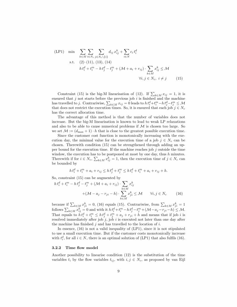
Since the customer cost function is monotonically increasing with the exe-cution day, the minimal value for the execution time of a job j ∈ Nc can bechosen. Therewith condition (15) can be strengthened through adding an up-per bound for the execution time. If the machine reaches job j outside the timewindow, the execution has to be postponed at most by one day, thus h minutes.Therewith if for i ∈ Nc,

∑k∈M xkij = 1, then the execution time of j ∈ Nc can

be bounded by

h tdi + tmi + ai + rij ≤ h tdj + tmj ≤ h tdi + tmi + ai + rij + h.

So, constraint (15) can be augmented by

h tdi + tmi − h tdj − tmj + (M+ ai + rij) ·∑k∈M

xkij

+(M− aj − rji − h) ·∑k∈M

xkji ≤M ∀i, j ∈ Nc (16)

because if∑k∈M xkji = 0, (16) equals (15). Contrariwise, from

∑k∈M xkji = 1

follows∑k∈M xkij = 0 and with it h tdi +tmi −h tdj −tmj +(M−aj−rji−h) ≤M.

That equals to h tdi + tmi ≤ h tdj + tmj + aj + rji + h and means that if job i isresolved immediately after job j, job i is executed not later than one day afterthe machine has finished j and has travelled to the location of i.

In essence, (16) is not a valid inequality of (LP1), since it is not stipulatedto use a small execution time. But if the customer costs monotonically increasewith tdi , for all i ∈ N , there is an optimal solution of (LP1) that also fulfils (16).

3.2.2 Time flow model

Another possibility to linearise condition (12) is the substitution of the timevariables ti by the flow variables tij , with i, j ∈ Nc, as proposed by van Eijl

9

(1995). These variables are always zero if xkij = 0, for all k ∈M . Contrariwise,

if any machine travels from job i to j, the pair tij := (tdij , tmij ) is the execution

time of job i. The corresponding linear model is

(LP2) min∑k∈M

∑i∈Nc

∑j∈Nc\{i}

dij xkij +

∑i∈N

ci ·∑j∈Nc

tdij (17)

s.t. (2)–(10)

td0 ·∑k∈M

xkij ≤ tdij ≤ dmax ·∑k∈M

xkij ∀i, j ∈ Nc (18)

0 ≤ tmij ≤ ui ·∑k∈M

xkij ∀i, j ∈ Nc (19)∑i∈Nc

tski = t0 ∀k ∈M (20)∑j∈Nc\{i}

(h tdij + tmij ) ≥∑

j∈Nc\{i}

(h tdji + tmji + (aj + rji) ·∑k∈M

xkji)

∀i ∈ N (21)

tdij ∈ N , tmij ∈ R+ ∀i, j ∈ Nc (22)

In the objective function, tdi is replaced by∑j∈Nc

tdij that represents theexecution day of job i. The route conditions are the same as in the basic three-index model (NLP), see constraints (2)–(10).

By means of conditions (18) and (19), it is ensured that tdij = tmij = 0 if j is

not the successor of i, thus if∑k∈M xkij = 0 with i, j ∈ Nc. Contrariwise, the

execution day is bounded by the start day td0 and the maximally allowed daydmax, and the execution minute is bounded by 0 and ui. Equation (20) definesthe execution time of the start depots. By condition (21), the correctness ofthe execution times is guaranteed. The left side is the execution time of jobi. The right side gives the execution time of the job resolved before i, becausethis is the only one where a k ∈ M exists such that xkji = 1 and, hence, the

only one with time variables tdji and tmji representing the execution time of thepredecessor of i. Condition (21) cannot be required for the depots, because astart depot has no predecessor and its execution time is fixed, and an end depothas no successor so that tzki = (0, 0), for all i ∈ Nc and k ∈M , as follows from(18) and (19). Since the customer costs of the depots are zero, the executiontime of the end depot must not be determined. If necessary, the definition ofan execution time for the end depots can be realised through small changes inthe route definition, e.g., adding an artificial travel from the end depot back tothe start depot.

The advantage of formulation (LP2) is that no big-M term is needed. But thenumber of time variables increases drastically. Instead of 2nc time variables, thismodel requires 2n2c . Also the number of constraints is increased, even though

10

the most of them are less complex.

3.2.3 Another Splitting of the Execution Time

To reduce the number of variables of the time flow model, the execution time inminutes tei = h tdi + tmi can be used instead of calculating it from the executionday and minute. With it, one flow variable teij is sufficient to determine the

execution time. The execution day tdi , necessary to calculate the customercosts, is the integer between 1

h

∑j∈N t

eij−1 and 1

h

∑j∈N t

eij . Since the execution

minute is bounded, the remainder of the division 1h

∑j∈N t

eij has to be at most

ui, for all i ∈ Nc.Therewith, the number of time variables is n2c +nc, a reduction compared to

(LP2), but some additional constraints are necessary to calculate the executionday.

(LP3) min∑k∈M

∑i∈Nc

∑j∈Nc\{i}

dij xkij +

∑i∈N

ci tdi

s.t. (2)–(10)

(h td0 + tm0 ) ·∑k∈M

xkij ≤ teij ≤ (h dmax + ui) ·∑k∈M

xkij

∀i, j ∈ Nc (23)∑i∈Nc

teski = h td0 + tm0 ∀k ∈M (24)∑j∈Nc\{i}

teij ≥∑

j∈Nc\{i}

(teji + (aj + rji) ·∑k∈M

xkji)

∀i ∈ N (25)

1h · (

∑j∈Nc

teij − ui) ≤ tdi ≤ 1h ·

∑j∈Nc

teij ∀i ∈ Nc (26)

teij ∈ R+ ∀i, j ∈ Nc (27)

tdi ∈ N ∀i ∈ Nc (28)

The objective function is equal to the objective function of (LP1). The exe-cution time in minutes teij is bounded by the start time in minutes h td0 + tm0 andh dmax + ui if any machine travels from job i to j, with i, j ∈ Nc. Contrariwise,teij = 0. These bounds are given by (23). By means of equation (24), the execu-tion times of the start depots are defined. Constraint (25) represents the timecondition (12) of the non-linear model (NLP). The execution of job i ∈ N can-not start before the execution of the previous job is finished and the machine hastravelled to the location of i. The execution day is defined by (26). Also the com-

11

pliance of the working shift is ensure. If the remainder of 1h ·

∑j∈Nc

teij is greater

than ui, there is no integer in the interval [ 1h · (∑j∈Nc

teij − ui), 1h ·∑j∈Nc

teij ].At last, the execution time in minutes teij are real numbers and the execution

days tdi are integers as defined by (27) and (28).Further formulations of the execution time are possible. For example the

second kind of splitting the execution time can also be used for the big-Mmodel of the time constraint. Another possibility to model the execution dayis the usage of binary variables dip that define that job i ∈ Nc is resolved onday p ∈ {td0, td0 +1, . . . , dmax}. That allows some additional constraints to theexecution times, e.g., if ai + min{rij , rji} + aj > 480, then the jobs i and jcannot be executed at the same day by the same machine. That can be definedby dip + djp ≤ 2 −

∑k∈M (xkij + xkji), for all p ∈ {td0, td0 + 1, . . . , dmax}. But for

the defined benchmarks, the working durations and travel times are too smallto formulate such constraints.

3.3 Alternative Route Formulations: Two-Index Models

To reduce the number of variables, the m routes of the m machines can be for-mulated as one large route through all depots with two-index binary variables.The variables xij code whether a machine travels from job i to job j. Addi-tionally, there are artificial travels from end depot zk to start depot sk+1, forall k = 1, 2, . . . ,m− 1, and from zm to s1. Then the routing constraints can bewritten as follows:

(LP4) min∑i∈Nc

∑j∈Nc\{i}

dij xij +∑i∈N

ci tdi (29)

s.t.∑

j∈Nc\{i}

xij = 1 ∀i ∈ Nc (30)∑j∈Nc\{i}

xji = 1 ∀i ∈ Nc (31)

xzms1 = 1 (32)

xzksk+1= 1 ∀k ∈M \ {m} (33)

xskzl = 0 ∀k, l ∈M (34)

xij ∈ {0, 1} ∀i, j ∈ Nc, ∀k ∈M (35)

12

vi ≤ nc − 1 ∀i ∈ Nc (36)

vs1 = 0 (37)

vi − vj + (nc − 1)xij ≤ nc − 2 ∀i, j ∈ Nc \ {s1} (38)

vsk ≥ vsk−1+ 3 ∀k ∈M \ {1} (39)

vi ∈ N ∀i ∈ Nc (40)

h tdj + tmj ≥ h tdi + tmi + ai + rij

∀i ∈ Nc, ∀j ∈ N \ {sk : k ∈M} : xij = 1 (41)

(11),(13),(14)

The equations (30) and (31) ensure that each job is visited and leaved ex-actly once. The artificial travellings between the depots are defined with (32)and (33). Empty routes are forbidden through (34). In the two-index routeformulation, the start depots have a predecessor in the route. Therewith thestart depots have to be excluded from the time constraints, see (41).

But constraints (30)–(35) are not sufficient to define a correct route throughall the depots in the correct order. Two problems occur: The first problem isthe order of the depots. It is possible to start in depot s1, visit some jobs and goto zk, k 6= 1, without visiting z1 or sk. Then the first machine starts in s1 butdoes not end in z1. And it is no problem to close the cycle, e.g. the depot orders1 . . . z2 s3 . . . z1 s2 . . . z3 fulfils all constraints but is not allowed. The secondproblem is that subtours are not avoided. In difference to the three-index models(LP1)–(LP3), the cycle C = {i1, i2, . . . , il} can contain depots. In the three-index models, this is impossible because start depots are only leaved and enddepots are only arrived. But in the two-index formulation, also the depots arearrived and leaved exactly once and therewith a subtour with depots is possible.Since the execution time of the start depots is fixed, the time constraint (41)must not be met and the contradiction tei1 < . . . < teil < tei1 of Lemma 1 isresolved in the start depot

tei1 < . . . < tezk 6< tesk+1< . . . < teil < tei1 .

So, additional constraints are necessary to exclude subtours and guarantee thecorrect order of the depots in the large route generated by the two-index vari-ables.

3.3.1 MTZ constraints

One possibility for a well-defined large route with two-index variables is theusage of the subtour elimination constraints from Miller, Tucker and Zemlin

13

(1960), see constraints (36)–(38), (40). The additional decision variable vi isthe position of job i ∈ Nc in the large route with s1 in position 0. By means ofcondition (38) is ensured that job j has a larger position than job i if xij = 1.If the route contains subtours, this condition leads to a contradiction and thesolution is infeasible. The chosen linearisation equals to a big-M formulationwith M = nc − 1. With the position variables vi can also be ensured that thestart depots are visited in the correct order, see constraint (39). Then the firstdepot reached after sk is the corresponding end depot zk and all jobs betweensk and zk are executed with machine k.

This route model can be combined with the time constraints of the threemodels (LP1)–(LP3) by replacing

∑k∈M xkij with xij and excluding the start

depots from constraint (15) when using (LP1).In Desrochers (1991), an improved formulation of the MTZ constraint is

given:

vi − vj + (nc − 1)xij + (nc − 3)xji ≤ nc − 2 ∀i, j ∈ Nc \ {s1} (42)

With it, two inequalities have to be considered if xij = 1, and it is vi ≤ vj − 1and vj ≤ vi + 1, thus vj = vi + 1.

3.3.2 Flow formulation of the MTZ constraints

Also the formulation of the MTZ constraints can be transformed in a flow modelto avoid the big-M term. Therefore the variables vi are replaced by the flowvariables vij with vij = 0 if xij = 0, and vij is the position of i (equals vi) ifxij = 1.

(LP5) min∑i∈Nc

∑j∈Nc\{i}

dij xij +∑i∈N

ci tdi

s.t. (30)–(35)

vs1i = 0 ∀i ∈ Nc (43)

vij ≤ (nc − 1)xij ∀i, j ∈ Nc \ {s1} (44)∑j∈Nc\{i}

vij =∑

j∈Nc\{i}

(vji + xji) ∀i ∈ Nc \ {s1} (45)∑i∈Nc

vski ≥∑i∈Nc

vsk−1i + 3 ∀k ∈M \ {1} (46)

vij ∈ N ∀i, j ∈ Nc (47)

(11), (41), (13), (14)

Equation (43) sets s1 as start of the job sequence. By means of constraint(44) is ensured that the position variable vij is zero if xij = 0. Otherwise, vij is

14

bounded by nc− 1. Equation (45) sets the position of job i by one greater thanthe position of the previous job. And (46) ensures the correct order of the startdepots.

As stated previously, the advantage of the flow formulation is that the big-M term is avoided at the expense of an increased number of variables andconstraints.

3.3.3 Binary machine allocation

Another possibility to avoid subtours and to guarantee the correct order of thedepots is the allocation of jobs to machines. The binary variable yik is 1 if job iis resolved by machine k, and 0 otherwise. Then, the problem can be modelledas

(LP6) min∑i∈Nc

∑j∈Nc\{i}

dij xij +∑i∈N

ci tdi

s.t. (30)–(35)∑k∈M

yik = 1 ∀i ∈ Nc (48)

yskk = 1 ∀k ∈M (49)

yzkk = 1 ∀k ∈M (50)

yik − yjk ≤ 1− xij∀k ∈M, i ∈ N ∪ {sk}, j ∈ N ∪ {zk} (51)

yik ∈ {0, 1} ∀i ∈ Nc, ∀k ∈M (52)

(11), (41), (13), (14)

Condition (48) ensures that each job is resolved by exactly one machine.The start and end depot of machine k are allocated to machine k, as definedwith (49) and (50). By constraint (51) is ensured that two successive resolvedjobs are resolved with the same machine. Therewith is guaranteed that alljobs allocated between the start depot sk and the end depot zk are resolvedwith machine k. Thus it is excluded to visit another depot before reachingzk. Also the occurrence of subtours is avoided: Assuming C := {i1, i2, . . . , il}is a cycle defined by the route variables. Because of the time constraints, Cmust contain depots (compare Lemma 1). Let iq−1 := zk−1 and iq := sk bethe depots. Then follows from (49), yskk := yiqk = 1 and from (51) thatyiqk = yiq+1k = . . . = yilk = yi1k = . . . = yiq−1k =: yzk−1k = 1. But (50) definesyzk−1k−1 = 1. Together with (48), this leads to a contradiction.

15

Condition (51) can also be formulated in a stronger way by

yik − yjk ≤ 1− xij − xji ∀k ∈M, i ∈ N ∪ {sk}, j ∈ N ∪ {zk}. (53)

3.3.4 Integer machine allocation

Instead of binary variables, also integer variables yi can be used to representthe machine allocation of job i ∈ Nc.

(LP7) min∑i∈Nc

∑j∈Nc\{i}

dij xij +∑i∈N

ci tdi

s.t. (30)–(35)

ysk = k ∀k ∈M (54)

yzk = k ∀k ∈M (55)

yi − yj ≤ (1− xij)m∀i ∈ N ∪ {sk : k ∈M}, ∀j ∈ N ∪ {zk : k ∈M} (56)

yi ∈ {1, 2, . . . ,m} ∀i ∈ Nc (57)

(11), (41), (13), (14)

Similar to (LP6), the depots sk and zk are resolved by machine k, definedwith constraints (54) and (55). Through (56) is ensured that each job is re-solved with a machine that has the same or a larger value than its predecessor.Therewith all jobs between sk and zk are resolved with the same machine k.Constraint (57) defines that yi is an integer with 1 ≤ yi ≤ m, for all i ∈ Nc. Asproposed in the binary machine allocation formulation, constraint (56) can bestrengthened by

yi − yj ≤ (1− xij − xji)m∀i ∈ N ∪ {sk : k ∈M}, ∀j ∈ N ∪ {zk : k ∈M} (58)

.Then, it is necessary to allocate each job to the same machine as the prede-

cessor since if xij = 1 two inequalities are considered and it follows yi − yj ≤ 0and yj − yi ≤ 0, i.e. yj = yi.

Compared to (LP6), the number of variables and constraints is reduced, butinteger variables are a bit more difficult because they can produce probablymore branching nodes.

16

4 Benchmarks

To test the performance of the different MILP formulations, 100 random bench-marks are created and solved. On request, these benchmark can be provided.Each benchmark contains 20 jobs randomly and non-clustered allocated in asquare of 100x100 points. The coordinates are given by uniformly distributedintegers in the interval [0, 100].The number of machines is selected from {2, 3, 4}and the execution starts with the working shift on the next day, so t0 := (1, 0).The x- and y-coordinates of the depots are chosen randomly in [25, 75]. There-with, the depots are allocated in an inner square of the map. All coordinatesare integers. The travel costs are the Euclidean distance multiplied with 10 androunded. The number of jobs afflicted with non-zero customer costs is brn ncfor a given random value rn ∈ [0.25, 0.75]. The amount of customer costs is alsochosen by random for each job that has non-zero customer costs, regulated bya given random value rc. Therewith the map contains jobs with high customercosts, but also jobs with low (and non-zero) customer costs. Thus, by means ofrn and rc very different benchmarks can be created. It is not possible, to knowin advance how big the influence of the customer costs is, but in general, a highvalue for rn leads to more jobs with non-zero customer costs and a high value forrc results in higher customer costs of the jobs. But the hardness of a benchmarkdoes not only depend on the number of jobs afflicted with customer costs andtheir values, but also on the allocation of the jobs and the depots on the map.If the jobs with high customer costs are far away from the start depots, thempreference leads to a long detour and the optimal solution differs more from theoptimal solution of the problem without customer costs. Contrariwise, if thejobs close to the start depots are afflicted with non-zero customer costs, the in-fluence of the customer costs on the solution is small. The reason is that also inthe problem without customer costs, these jobs are scheduled at the beginningof the planning process.

5 Solving Method

In order to tight the MILP formulations of the VRP-CC, we use an approachknown from solving the Travelling Salesmen Problem (TSP), which is very closeto VRPs. It has been shown, that the subtour elimination constraints fromDantzig, Fulkerson and Johnson (1954), in the following called DFJ constraints,are better than the subtour elimination constraints from Miller, Tucker andZemlin (1960) used in (LP4) and similar to the time constraints. The DFJconstraints are formulated as follows:∑

i,j∈Sxij ≤ |S| − 1 ∀S ⊂ Nc, |S| > 1 (59)

Constraint (59) guarantees that S is not a subtour, since, if S is a subtour, thenfor all i ∈ S, and q ∈ Nc \ S is xiq = 0. Consequentially

∑j∈S xij = 1, for all

i ∈ S, and therewith∑i,j∈S xij = |S|. The DFJ constraints lead to a stronger

17

formulation than the MTZ constraints; they are even facets of the polytope ofthe TSP (Nemhauser, 1988). The disadvantage of the DFJ constraints is thehigh number of subsets S that have to be probed. Even it is sufficient to test allsubsets with 2 ≤ |S| ≤ nc

2 , since if S is a subtour, then also Nc \ S, the numberof subsets is exponentially in the number of jobs.

An elementary approach to tighten the TSP formulation with MTZ con-straints is the step-by-step inclusion of DFJ constraints for occurring subsets(Pataki, 2003). At first, the TSP is solved without any subtour eliminationconstraints. The obtained solution normally contains subtours (if not, it is anoptimal solution and the solving process can be stopped). Based on these sub-tours, DFJ constraints are generated in order to avoid their occurrence in furthersolving steps. With this small selection of DFJ constraints, the integer problemis solved again. The steps “solving” and “adding DFJ constraints” are repeatedβ-times (or until the obtained solution does not contain subtours). If in the βruns no solution without subtours was found, the MTZ constraints are added.The problem containing the MTZ constraints and also the generated set of DFJconstraints is solved to obtain an optimal solution. As computational tests haveshown, using such a small set of DFJ constraints leads to better running timesthan solving the problem without any DFJ constraints.

To use this approach, the time constraints have to be relaxed because theywork as MTZ constraints and does not allow any subtours (see Lemma 1).Therefore, the time constraints are only added for a small subset of jobs withhigh customer costs NT ⊂ N with ci ≥ cj , ∀i ∈ NT , j ∈ Nc \ NT and|NT | = (n+m)α with α ∈ [0, 1] a chosen value. So, in (LP1) the time con-straints (15) are limited to

h tdj + tmj ≥ h tdi + tmi + (M+ ai + rij) ·∑k∈M

xkij −M ∀i ∈ Nc, j ∈ NT .

The other time formulation variants are relaxed in the same way, only for thejobs j ∈ NT is stipulated that its execution starts not before the previous jobis finished and the machine reaches j. In the two-index route formulation, theadditional part to avoid subtours and to guarantee the correct depot order isalso omitted, thus the variables v respectively y do not occur. The relaxedproblem is solved β-times. The occurring subtours are the base of the DFJconstraints. The DFJ constraints are generated for the union of at most γsubtours of the current solution and added before the relaxed problem is solvedagain. Therewith, in every run new subtours occur and new DFJ constraintsare formulated. After at most β runs or if the solution of the relaxed problemdo not contain further subtours, the VRP-CC formulation is augmented by thegenerated DFJ constraints and solved. The solution method is shown as pseudocode in Algorithm 1. The procedure of generating DFJ constraints is calledpreprocess.

Different tests were necessary to get suitable values for α, β and γ. Clear isthat the higher α, the smaller is the number of occurring subtours since eachsubtour must contain at least one job without time constraints. If β and γ are

18

Algorithm 1: Base solving framework

Input: MILP formulation of VRP-CC# Define NTNT ⊂ Nc with ci ≥ cj , ∀i ∈ NT , j ∈ Nc \NT and |NT | = nα# Store the subsets for DFJ constraintsS := ∅Do β-times

Solve relaxed problemwith DFJ constraints

∑i,j∈S xij ≤ |S| − 1 ∀S ∈ S

Let S1, S2, . . . , Sl be the subtours of the solutionif l=1 then

returnelse

forall the P ∈ P({1, 2, . . . , l}) with 1 ≤ |P | ≤ min{γ, l − 1} doS := S ∪ {

⋃p∈P Sp}

end

end

endSolve the MILP formulation of the VRP-CC

with the additional DFJ constraints∑i,j∈S xij ≤ |S| − 1 ∀S ∈ S

chosen small, only less runs are made to generate DFJ constraints, and basedon a given set of subtours only less DFJ constraints are included. Therewiththe final problem contains only less additional DFJ constraints that leads toa smaller improvement in the running time. Contrariwise, if β is chosen high,only less DFJ constraints are generated in the last runs since only less subtoursoccur and mostly subtours similar to the previous runs. Therewith similar DFJconstraints are generated that could not further tight the LP relaxation butincreases the number of constraints. Also a high value for γ leads to an increasein the calculation effort. DFJ constraints of large subsets S seem to have aworse performance.

To show the advantage of adding DFJ constraints, the average results ofsolving the 100 random benchmarks are presented in Table 1 for different valuesof α. For the calculation we used β = γ = 3 and (LP1). Shown is the averagerunning time for the whole solving process, the preprocessing time that is thetime to generate the DFJ constraints, the number of obtained DFJ constraintsand the number of runs therefore, and at last the number of optimal solvedproblems during the time limit of 15 minutes. In the case α = 1, no runs togenerate DFJ constraints are necessary since the time constraints prohibit theoccurrence of subtours. Thus β = 0.

The results show the high profit of adding DFJ constraints. Comparing therunning time of α = 0.75, where only less DFJ constraints are generated, andα = 1, a small improvement in the running time and a significant increasing

19

α 0.0 0.25 0.5 0.75 1.0Solving Time (sec) 130 131 138 195 220Preprocessing Time (sec) 0.19 0.25 0.47 9.71 -DFJ Constraints 86 74 42 6 -Solved problems 92 93 91 89 59

Table 1: Average results of 100 random benchmarks for different α.

in the number of solved problems can be seen. So, even this very small set ofDFJ constraints strengthened the formulation to improve the performance inCPLEX. The performance can be further improved by decreasing α because oftwo reasons: On the one hand, a smaller α leads to a smaller preprocessingtime, thus less time is necessary to solve the relaxed problems to create DFJconstraints. And on the other hand, a small α leads to more subtours andwith it more DFJ-constraints are generated. And the more DFJ constraints,the stronger is the LP relaxation. But more constraints can also lead to morecalculation effort. With α = 0 and α = 0.25, the performance is similar, even thenumber of DFJ constraints differs. Since with α = 0.25, one more benchmarkwas solved, we decide to use this value in further calculations.

6 Results

The tests were executed on a PC with an Intel 2.8Ghz Quad-Core, 8GB RAMand Windows 7 (64-bit). The 64-bit version of CPLEX 12.5 was used as MILPsolver with its default settings. The solving time was limited to 15 minutes inall benchmarks.

6.1 Time Formulations

At first, the different formulations of the time constraints are compared:• the big-M formulation (LP1)• the big-M formulation with strengthened constraints, see (LP1) and (16)• the flow model (LP2) with execution day and execution minute• the flow model (LP3) with execution time in minutes and resultant exe-

cution dayTable 2 shows the average solving time, the average number of CPLEX nodesand iterations, the number of optimal solved problems, and the quality of theLP bound that is the average distance of the LP bound to the optimal valuein per cent. For the test, we used the preprocessing parameters α = 0.25 andβ = γ = 3.

The results show that the big-M formulation with 2nc time variables has thebest performance in CPLEX. The average solving time is significant smaller thanthe average solving times of the other variants to formulate the time conditions,and 92 of the 100 benchmarks are solved optimally during the time limit of 15minutes.

20

(LP1) (LP1) (LP2) (LP3)strength.

Solving Time (sec) 136 150 287 223Nodes (in th.) 386 378 192 242Iterations (in th.) 4480 4801 10074 10929Solved problems 92 88 81 88Quality of LP bound 20 12 19 20

Table 2: Average results of 100 random benchmarks for the three-index modelwith different time formulations.

The strengthened variant of (LP1), with a more limited execution time,leads to a better LP bound and to a small reduction in the number of analysedbranching nodes. But in each branching node, the linear relaxation has moreconstraints that leads to a higher solving effort. This can be seen in the highernumber of iterations and the greater average solving time.

The both variants (LP2) and (LP3) with the flow formulation of the timeconstraints are also less successful than (LP1). The advantage was to avoid thebig-M formulation because it leads to weak LP relaxations. But the increase invariables and constraints leads to greater problem sizes in the LP relaxation andtherewith to more calculation effort. That can be seen in the high numbers ofiterations compared to the smallish number of branching nodes. The reductionof branching nodes is an indicator for better LP bounds, even if the initialbound is similar to the bound from (LP1). The high increasing in iterationsshow the high computational effort to solve the LP relaxations. All in all, theperformance in CPLEX of the flow formulations is worse than the performanceof (LP1).

To ensure that (LP1) has the best performance not only because the pre-processing parameters were obtained with this formulation, we made some testswith other preprocessing parameters; all showed similar results.

6.2 Route Models

After the best formulation for the time constraint was found, the different routeformulations were compared against each other. Based on the high differencein the route definition, the two-index route formulation leads to more subtoursusing the parameters obtained with (LP1). But different tests have shown thatα = 0.25 and β = γ = 3 are also suitable for the two-index route formula-tions (LP4)–(LP7). The two-index formulations are completed with the timeformulation of (LP1).

In Table 3, the route formulations (LP4)–(LP7) are compared with the three-index model (LP1). Table 4 contains the results of the strengthened variants ifexist. Thus in (LP4), constraint (38) is replaced by (42), and in (LP6) and (LP7)the constraints (53) and (58) are used instead of (51) and (56). Shown are theaverage solving time in seconds, the number of analysed branching nodes and

21

the number of iterations in thousands, the number of optimal solved problemsduring 15 minutes, and the quality of the LP bound that is the average distanceof the LP bound and the optimal value in per cent.

(LP1) (LP4) (LP5) (LP6) (LP7)Solving Time (sec) 136 118 136 103 100Nodes (in th.) 386 298 238 225 313Iterations (in th.) 4480 4017 6110 3486 4082Solved problems 92 93 94 95 95Quality of LP Bound 20 22 21 21 22

Table 3: Average results of 100 random benchmarks for different route formu-lations with the big-M time formulation.

The results show that the performance of the two-index formulations heavilydepends on the selected variant to avoid subtours and to ensure the correct orderof the depots even all of them have nearly the same LP bound quality.

Comparing the average values of two variants of the MTZ constraints, itcan be seen that the flow formulation of (LP5) is not better than the commonvariant (LP4) with the big-M formulation. The results are similar to the caseof the time constraint as big-M formulation and flow formulation. In both, withthe flow formulation less branching nodes are analysed, but the effort to solvethe problem of a branching node is higher. Overall, the solution effort is higherand the big-M formulation should be preferred.

The machine allocation variants (LP6) and (LP7) have nearly the samerunning time. Using binary machine allocation variables results in a highernumber of variables and constraints; and therewith in more rows and columnsof the LP relaxation. Using integer variables reduces the problem size, but oftenmore branchings are necessary to define an integer variable and therefore thenumber of branching nodes increases. These effects can be seen when comparingthe number of nodes and iterations. By solving the problem with the (LP7)formulation, more branching nodes are analysed. But the LP relaxations aresolved faster. So, (LP7) with integer variables has a better performance than(LP6) with binary variables.

(LP1) (LP4) (LP5) (LP6) (LP7)strength. strength. strength.

Solving Time (sec) 136 120 136 100 85Nodes (in th.) 386 303 238 247 242Iterations (in th.) 4480 4444 6110 3582 3347Solved problems 92 95 94 95 94Quality of LP Bound 20 14 21 21 13

Table 4: Average results of 100 random benchmarks for different strengthenedroute formulations with the big-M time formulation.

The results presented in Table 4 show the benefit from strengthen the addi-

22

tional constraints of the two-index formulations.Looking to (LP4) and its strengthened variant shows that the solving time,

number of analysed branching nodes and number of iterations are increasedalthough the LP bound of the root problem is much better. But with thestrengthened variant, two more benchmarks are solved during the 15 minutetime limit. Overall, both seem to have a similar performance.

The machine allocation variants show very different impacts of strengthenconstraint (53) or (58), although the strengthening is very similar. Strengthen(LP6) does not improve the LP bound and the time required for solving. Incontrast, (LP7) is much improved through strengthening. The solving timeis reduced significantly, less branching nodes are analysed, less iterations werenecessary to solve the relaxed problems and the LP bound of the root is better.With it, the integer variant of the machine allocation formulation is much betterthan the variant with binary variables.

All in all, the best results are obtained with the integer machine allocationformulation (LP7). In general, the two-index formulations are better than thethree-index formulation.

6.3 Benchmark characteristics

At last, we want to show the influence of benchmark characteristics to theperformance. Therefore, the 100 random benchmarks were clustered dependenton the ratio of customer costs in the optimal solution value and dependent on thedetour length that is the increase in travel costs of the optimal value comparedto the optimal value of the same benchmark without customer costs. The resultsare shown in Figure 1 for the three MILP formulations (LP1), (LP4) and thestrengthened variant of (LP7). On the left side, the average solving time of thebenchmarks that belong to the different customer cost groups are pictured, andthe right side shows the average running times of the benchmarks that belongto different groups of the detour length. To get the groups for the ratio ofcustomer costs, the benchmarks were sorted by the ratio of customer costs inthe optimal solution. Then, the benchmarks of the first group are the first fifthof the sorted benchmarks, the benchmarks of the second group are the secondfifth, and so on. In the same way, with a sorting based on the length of thedetour, the groups that belongs to the detour length are generated. The barsrepresent the average running time of the MILP formulation. They are plottedon the x-coordinate that is the average ratio of costumer costs or the averagedetour length of the group.

It can be seen that with increasing ratio of customer costs the benchmarksare harder to solve. All three MILP formulations requires more time to solvethe benchmarks of the last two customer cost groups. The results of (LP4) inFigure 1 show that (LP4) is worse than (LP1) in the benchmarks with a lowratio of customer costs. In contrast, (LP1) needs more time than (LP4) to solvebenchmarks with a high ratio of customer costs. In each group, the strengthenedvariant of (LP7) has the smallest average running time.

Grouping the benchmarks by the detour length leads to similar results,

23

Figure 1: Dependence of solving time on benchmark characteristics.

benchmarks with small length of detour are solved faster than benchmarkswhere a long detour was necessary to reduce customer costs. It seems that(LP1) works worse for benchmarks with very short or very long detours, andthat (LP4) is worse by medium length of detour. Again, in each group (LP7)in its strengthened variant has the best performance.

Overall, the solution quality depends on both, the ratio of customer costsand the detour length. The group allocation of the benchmarks is different inthe both criteria. The reason is that there are benchmarks with a small ratioof customer costs where a long detour is necessary to get this small value. Andthere are also benchmarks, where the jobs are afflicted with high customer costsbut this has hardly influence in the route of the optimal solution. Then thedetour length is small, but the ratio of costumer costs in the optimal value canbe high.

7 Conclusion

Our research has shown that the new kind of cost function in the VRP leadsto problems harder to solve. The higher the customer costs, the more time isrequired to solve the problem with CPLEX even when only a small ratio of jobsis afflicted with non-zero customer costs. So, the VRP-CC is a new challengein VRP.

The results also show the influence of the problem formulation to the perfor-mance in CPLEX. In practise, different MILP formulations should be developedand compared to solve a problem as efficiently as possible with a MILP solver.

In real applications, different additional restrictions can occur. One exampleis a limited capacity of the machines. In the presented models is only stipulatedthat each machine serves at least one job. But in reality, it will be betterto split the jobs evenly over all machines. This can be realised by choosingdmax smaller, but it will be hard to find a suitable value to ensure that theproblem is not infeasible and to restrict the machine capacity. Better ways arerestrictions in the number of jobs served by a machine or the pure working timeof the machines. It is easy to include such constraints in the three-index modelsince the three-index binary variables are a good link between a machine and

24

the jobs allocated to it. But for some two-index models, regarding capacityconstraints can be difficult. For example, the condition “each machine canresolve at most K jobs” can be ensured very simple with the MTZ constraints(vzk − vsk ≤ K + 1). But a condition “the pure working time of a machine isat most T hours” requires binary variables for the machine allocation becausethe working times of the jobs allocated to a machine must be summed. Besidethe three-index formulation, (LP6) is able to handle such constraints withoutadditional variables.

In practise, the number of jobs is much higher than 20. To solve biggerproblems, heuristics and meta-heuristics are necessary because MILP solverrequires too much time for solving. But they can be used as part of a meta-heuristic, e.g., in a multi-level approach. There, jobs are merged to a small setof superjobs. A solution of the resulting VRP-CC for the superjobs can be foundwith a MILP solver. Also the order of resolving the jobs merged to a superjobcan be obtained by means of a MILP solver.

References

Clarke G, Wright JW (1964) Scheduling of vehicles from a central depot to anumber of delivery points. Operations Res, 12(4), 568-581.

Dantzig GB, Fulkerson DR, Johnson SM (1959) Solution of a large-scaletraveling-salesman problem. J of the Operations Res Society of Am, 393-410.

Desrochers M, Laporte G (1991). Improvements and extensions to the Miller-Tucker-Zemlin subtour elimination constraints. Operations Res Letters, 10(1),27-36.

Baldacci R, Christofides N, Mingozzi A (2007) An exact algorithm for the vehiclerouting problem based on the set partitioning formulation with additionalcuts. Mathematical Programming, 115(2), 351-385.

Eksioglu B, Vural AV, Reisman A (2009) The vehicle routing problem: Ataxonomic review. Computers and Industrial Engineering, 57(4), 1472-1483.doi:10.1016/j.cie.2009.05.009

Gillett BE, Miller LR (1974) A heuristic algorithm for the vehicle-dispatch prob-lem. Operations Res, 22(2), 340-349.

Heinicke F, Simroth A, Tadei R, Baldi MM (2013) Job order assignment atoptimal costs in railway maintenance. Proc of the 2nd Int Conf on OperationsRes and Enterpr Syst (ICORES2013).

Heinicke F, Simroth A (2013) Application of Simulated Annealing to RailwayRoutine Maintenance Scheduling. 14th Int Conf on Civ, Struct and EnvironEng Comp.

25

Kumar SN, Panneerselvam R (2012) A Survey on the Vehicle Routing Problemand Its Variants. Intelligent Information Management, 4(3), 66-74.

Laporte G (2007) What you should know about the vehicle routing problem.Naval Research Logistics (NRL), 54(8), 811-819.

Macedo R, Alves C, Valerio de Carvalho JM, Clautiaux F, Hanafi S.(2011)Solving the vehicle routing problem with time windows and multiple routesexactly using a pseudo-polynomial model. EJOR, 214(3), 536-545.

Miller, C. E., Tucker, A. W., Zemlin, R. A. (1960). Integer programming for-mulation of traveling salesman problems. JACM, 7(4), 326-329.

Miwa M (2002) Mathematical programming model analysis for the optimaltrack maintenance schedule. Quarterly Report of RTRI, 43(3), 131-136.doi:10.2219/rtriqr.43.131

Nemhauser GL, Wolsey LA (1988) Integer and combinatorial optimization. NewYork: Wiley.

Oyama T, Miwa M (2006) Mathematical modeling analyses for obtaining anoptimal railway track maintenance schedule. Jpn J of ind and appl math,23(2), 207-224. doi:10.1007/BF03167551

Pataki G (2003) Teaching integer programming formulations using the travelingsalesman problem. SIAM review, 45(1), 116-123.

Quiroga LM, Schnieder E (2010) A heuristic approach to railway track mainte-nance scheduling. Proc of 12th Int Conf on Computer Syst Des and Operationin Railw and Other Transit Systems, 687699, China.

Tan KC, Lee LH, Zhu QL, Ou K (2001) Heuristic methods for vehicle routingproblem with time windows. Artif Intell in Eng, 15(3), 281-295.

Vale C, Ribeiro I, Calcada R (2012) Integer Programming to Optimize Tampingin Railway Tracks as Preventive Maintenance. J Transp Eng, 138(1), 123-131.doi:10.1061/(ASCE)TE.1943-5436.0000296

Van Eijl CA (1995) A polyhedral approach to the delivery man problem. Techni-cal Report 95-19, Department of Mathematics and Computing Science, Eind-hoven University of Technology.

26