On a family of finite moving-average trend filters for the ...

Journal of ForecastingJ. Forecast. 21, 125–149 (2002)Published online 17 January 2002 in Wiley InterScience (www.interscience.wiley.com). DOI: 10.1002/for.817

On a Family of Finite Moving-averageTrend Filters for the Ends of Series

ALISTAIR G. GRAY1 AND PETER J. THOMSON2*1 Statistics New Zealand, Wellington, New Zealand2 Statistics Research Associates Ltd, Wellington, New Zealand

ABSTRACTA family of finite end filters is constructed using a minimum revisions cri-terion and based on a local dynamic model operating within the span of agiven finite central filter. These end filters are equivalent to evaluating thecentral filter with unavailable future observations replaced by constrainedoptimal linear predictions. Two prediction methods are considered: best lin-ear unbiased prediction and best linear biased prediction where the bias istime invariant. The properties of these end filters are determined. In partic-ular, they are compared to X-11 end filters and to the case where the centralfilter is evaluated with unavailable future observations predicted by globalARIMA models as in X-11-ARIMA or X-12-ARIMA. Copyright 2002John Wiley & Sons, Ltd.

KEY WORDS local dynamic model; minimum revisions; best linear unbiasedprediction; best linear biased prediction

INTRODUCTION

Many seasonal adjustment procedures decompose time series into trend, seasonal, irregular andother components using non-seasonal finite moving-average trend filters. This paper is concernedwith the extension of the finite central moving-average trend filter used in the body of the series tothe ends where there are missing observations.

For any given finite central moving-average trend filter, a family of end filters is constructedusing a minimum revisions criterion and a local dynamic model operating within the span ofthe central filter. These end filters are equivalent to evaluating the central filter with unavailablefuture observations replaced by constrained optimal linear predictors. Two prediction methods areconsidered: best linear unbiased prediction (BLUP) and best linear biased prediction, where the biasis time invariant (BLIP). The BLIP end filters are shown to be a generalization of those developedby Musgrave (1964) for the central X-11 Henderson filters and include the BLUP end filters as aspecial case.

* Correspondence to: Peter Thomson, Statistics Research Associates Ltd, PO Box 12649, Thorndon, Wellington, NewZealand. E-mail: [email protected]/grant sponsor: ASA/NSF/Census.

Received February 1999Revised March 2000

Copyright 2002 John Wiley & Sons, Ltd. Accepted June 2001

126 A. G. Gray and P. J. Thomson

The theoretical properties of BLUPs and BLIPs are examined. In particular, it is establishedthat the BLIP end filters generally have smaller mean squared revisions than the BLUP end filters.However, unlike the BLUP filters, the BLIP filters are no longer independent of the parametersin the local dynamic model and so, in practice, it is possible that a mis-specification of theseparameters will lead to BLIP end filters with greater mean squared revisions than BLUP end filters.The effects of such mis-specification are discussed. Comparisons are also made between these endfilters and the Musgrave end filters used by X-11, and the end filters obtained when the centralfilter is evaluated with unavailable future observations predicted by global ARIMA models. Thelatter parallels the ARIMA forecast extension method used in X-11-ARIMA (Dagum, 1980) andX-12-ARIMA (Findley et al, 1998). Finally these filters are evaluated on some New Zealand timeseries.

LOCAL DYNAMIC MODEL

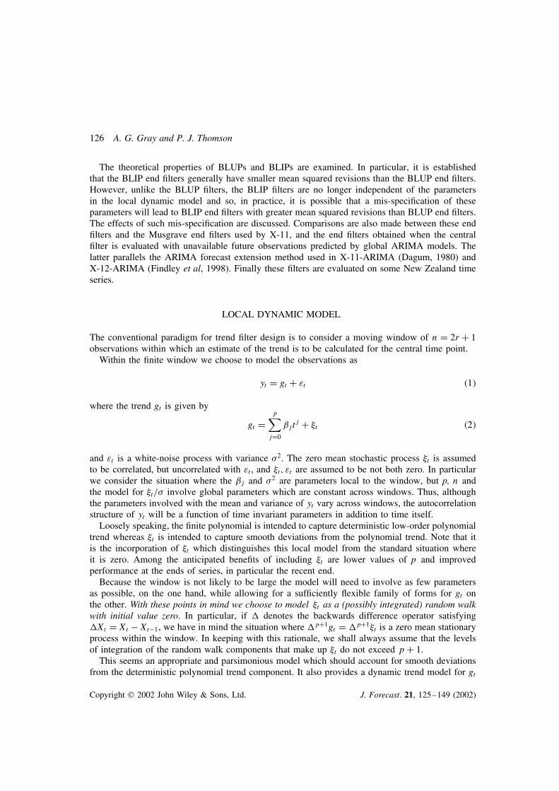
The conventional paradigm for trend filter design is to consider a moving window of n D 2r C 1observations within which an estimate of the trend is to be calculated for the central time point.

Within the finite window we choose to model the observations as

yt D gt C εt �1�

where the trend gt is given by

gt Dp∑jD0

ˇjtj C �t �2�

and εt is a white-noise process with variance 2. The zero mean stochastic process �t is assumedto be correlated, but uncorrelated with εt, and �t, εt are assumed to be not both zero. In particularwe consider the situation where the ˇj and 2 are parameters local to the window, but p, n andthe model for �t/ involve global parameters which are constant across windows. Thus, althoughthe parameters involved with the mean and variance of yt vary across windows, the autocorrelationstructure of yt will be a function of time invariant parameters in addition to time itself.

Loosely speaking, the finite polynomial is intended to capture deterministic low-order polynomialtrend whereas �t is intended to capture smooth deviations from the polynomial trend. Note that itis the incorporation of �t which distinguishes this local model from the standard situation whereit is zero. Among the anticipated benefits of including �t are lower values of p and improvedperformance at the ends of series, in particular the recent end.

Because the window is not likely to be large the model will need to involve as few parametersas possible, on the one hand, while allowing for a sufficiently flexible family of forms for gt onthe other. With these points in mind we choose to model �t as a (possibly integrated) random walkwith initial value zero. In particular, if denotes the backwards difference operator satisfyingXt D Xt � Xt�1, we have in mind the situation where pC1gt D pC1�t is a zero mean stationaryprocess within the window. In keeping with this rationale, we shall always assume that the levelsof integration of the random walk components that make up �t do not exceed pC 1.

This seems an appropriate and parsimonious model which should account for smooth deviationsfrom the deterministic polynomial trend component. It also provides a dynamic trend model for gt

Copyright 2002 John Wiley & Sons, Ltd. J. Forecast. 21, 125–149 (2002)

Finite Moving-average Trend Filters 127

which is essentially of the same form as that used in the global structural models that have beensuccessfully applied to economic and official data. See Akaike (1980), Schlicht (1981), Hillmerand Tiao (1982), Gersch and Kitagawa (1983), Bell and Hillmer (1984), Harvey (1989), Maravall(1993), and Young et al. (1999) for example. For these global models there is no need for specialend filters since they are automatically provided using the global model and, in most cases, recursivealgorithms such as the Kalman filter and smoother. The final trend filters implied by these globalprocedures are infinite central moving-average filters. By contrast, here we consider local models andthe situation where the central moving-average trend filters are finite as is the case in X11-ARIMA,X-12-ARIMA, SABL (Cleveland et al, 1978) and STL (Cleveland et al, 1990).

In the local linear case p D 1 a simple dynamic model for gt is given by

yt D gt C εt D ˇ0 C ˇ1t C �t C εt �3�

where ˇ0, ˇ1 are constants and �t is a simple random walk satisfying

�t D �t�1 C �twith �0 D 0. Here gt D ˇ1 C �t and εt, �t are mutually uncorrelated white-noise processes withvariances 2 and 2

� D � 2 respectively. In the local quadratic case p D 2 a simple dynamic modelfor gt is given by

yt D gt C εt D ˇ0 C ˇ1t C ˇ2t2 C �t C εt �4�

where ˇ0, ˇ1, ˇ2 are constants and �t is a simple random walk satisfying the same conditions as inthe local linear model. Preliminary analysis indicates that these models have properties that can beregarded as representative of other more general models of the type discussed above.

TREND FILTER DESIGN AT THE ENDS

Now consider a finite window of width n D 2r C 1 points centred at time point t and within whichthe observations follow the local dynamic model given in the previous section. We consider thecase where the trend gt is to be estimated by a given finite central moving-average trend filter

Ogt Dr∑

sD�rwsytCs �5�

In keeping with standard practice, we assume that the ws are constrained by the requirement that

EfOgt � gtg D 0 �6�

so that Ogt is an unbiased estimator of gt. Note that this condition is equivalent to the requirementthat the ws satisfy

r∑sD�r

ws D 1r∑

sD�rsjws D 0 �0 < j � p� �7�

so that the moving-average filter passes polynomials of degree p.



At the ends of series the central moving-average filter (5) will involve unavailable futureobservations. How these missing observations should be treated is open to question.

A common and natural approach involves forecasting the missing values, either implicitly orexplicitly, and then applying the desired central filter. The forecasting methods used range fromsimple extrapolation to model-based methods, some based on the local trend model adopted, otherson global models for the series as a whole. The latter include the fitting of ARIMA models toproduce forecasts (see Dagum, 1980 in particular). The principle of using prediction at the ends ofseries seems a key one which goes back to DeForest (1877). See also the discussion in Cleveland(1983), Greville (1979) and Wallis (1983).

Yet another way to handle the missing values in the window is to employ additional criteriaspecific to the ends of the series. An important requirement, especially among official statisticians,is to keep seasonal adjustment revisions and therefore trend revisions to a minimum as more datacomes to hand. Thus, at the ends of series, a natural criterion to consider is

Rq D E

(

r∑sD�r

wsytCs � Qgt)2 �8�

where Qgt is a predictor of Ogt D ∑rsD�r wsytCs based on the data available. In general, given a history

of observations y1, . . . , yT, it is evident that Rq is minimized when

Qgt Dr∑

sD�rws OytCs �9�

where OytCs D E�ytCsjy1, . . . , yT� denotes the best predictor of ytCs in the usual mean squared errorsense. Thus there is a close relationship between the minimum revisions approach and that offorecasting the missing values in the window.

The minimum revisions strategy appears to have been originally proposed by Musgrave (1964)for the case where Qgt is restricted to be linear in the observations within the window. (See thediscussion in Doherty, 1991.) This approach has also been used by Lane (1972), Laniel (1986)and will also be adopted here. Geweke (1978) and Pierce (1980) established the result (9) forthe case where Qgt is linear in past values of the time series (not just those within the win-dow) and where the time series follows an appropriate global model. However the argumentleading to (9) shows that in general OytCs, and hence Qgt, need not necessarily be linear in theobservations.

In this paper we adopt the minimum revisions strategy based on the moving window paradigmand the local dynamic trend model of the previous section. At the ends of the series we choose topredict Ogt D ∑r

sD�r wsytCs by a linear predictor of the form

Qgt Dq∑

sD�rusytCs �10�

where q D T� t with 0 � q < r, T denotes the time point of the last observation and the us aredependent on q. We shall consider two cases. The first imposes the condition that Qgt be an unbiasedpredictor of

∑rsD�r wsytCs. The second weakens this requirement by considering biased predictors

such as those developed by Musgrave (1964) for X-11 (see in particular Doherty, 1991).



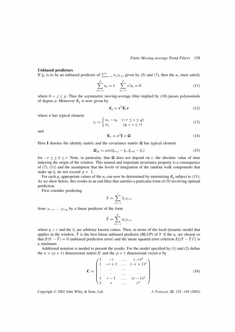
Unbiased predictorsIf Qgt is to be an unbiased predictor of

∑rsD�r wsytCs given by (5) and (7), then the us must satisfy

q∑sD�r

us D 1q∑

sD�rsjus D 0 �11�

where 0 < j � p. Thus the asymmetric moving-average filter implied by (10) passes polynomialsof degree p. Moreover Rq is now given by

Rq D vTE1v �12�

where v has typical element

vs D{ws � us ��r � s � q�ws �q < s � r� �13�

andE1 D 2I CZ �14�

Here I denotes the identity matrix and the covariance matrix Z has typical element

Zjk D cov��tCj � �t, �tCk � �t� �15�

for �r � j, k � r. Note, in particular, that Z does not depend on t , the absolute value of timeindexing the origin of the window. This natural and important invariance property is a consequenceof (7), (11) and the assumption that the levels of integration of the random walk components thatmake up �t do not exceed pC 1.

For each q , appropriate values of the us can now be determined by minimizing Rq subject to (11).As we show below, this results in an end filter that satisfies a particular form of (9) involving optimalprediction.

First consider predicting

Y Dr∑

sD�rυsytCs

from yt�r, . . . ytCq by a linear predictor of the form

OY Dq∑

sD�rusytCs

where q < r and the υs are arbitrary known values. Then, in terms of the local dynamic model thatapplies in the window, OY is the best linear unbiased predictor (BLUP) of Y if the us are chosen sothat E�Y� OY� D 0 (unbiased prediction error) and the mean squared error criterion Ef�Y� OY�2g isa minimum.

Additional notation is needed to present the results. For the model specified by (1) and (2) definethe nð �pC 1� dimensional matrix C and the pC 1 dimensional vector c by

C D

1 �r . . . ��r�p1 �r C 1 . . . ��r C 1�p

Ð Ð . . . ÐÐ Ð . . . Ð1 r � 1 . . . �r � 1�p

1 r . . . rp

�16�



and c D �1, 0, . . . , 0�T. Also, define the nð �q C r C 1� matrix L1 and the nð �r � q� matrix L2

by the relationI D [L1,L2] �17�

We now establish the following result.

Theorem 1 Let yt follow the local dynamic model specified by (1) and (2). Given υ D�υ�r, . . . , υr�T and observations yt�r, . . . , ytCq for 0 � q < r, the BLUP of

∑rsD�r υsytCs is∑q

sD�r usytCs where u D �u�r, . . . , uq�T is given by

u D LT1 �I � GL2�LT2 GL2��1LT2 �υ

HereG D E�1

1 � E�11 C�CTE�1

1 C��1CTE�11

E1 is given by (14) and C is given by (16).In particular the BLUP of

∑rsD�r υsytCs is given by

∑rsD�r υs OytCs where OytCs is the BLUP of ytCs

for q < s � r and ytCs otherwise.

Proof For OY D ∑qsD�r usytCs to be an unbiased predictor of Y D ∑r

sD�r υsytCs the us must satisfy

q∑�rsjus D

r∑�rsjυs �0 � j � p�. �18�

Given (18)

Y� OY Dr∑

sD�rvs��tCs � �t C εtCs�

where

vs D{υs � us ��r � s � q�υs �q < s � r� �19�

andr∑

�rsjvs D 0 �0 � j � p� �20�

In terms of the vs these conditions can be written as

LT2 v D LT2 υ CTv D 0 �21�

where v D �v�r, . . . , vr�T and C is given by (16). We now need to minimize

Ef�Y� OY�2g D vT� 2I C �v D vTE1v �22�

subject to (21).



Using Lagrange multipliers, optimizing with respect to the vs, and incorporating the constraints(21) yields the equations

v D E�11 C!C E�1

1 L2"

LT2 E�11 C!C LT2 E�1

1 L2" D LT2 υ

CTE�11 C!C CTE�1

1 L2" D 0

where !, " are the vectors of Lagrange multipliers. These together with (19) yield

u D LT1 �I � GL2�LT2 GL2��1LT2 �υ

as stated.Now the BLUP of ytCs is obtained by setting υ D 0 with the exception of the sth element which

is set to unity. Then the BLUP of ytCs is given by

OytCs D{ytCs ��r � s � q�hTs y �q < s � r�

where hs is the sth column of �LT1 GL2�LT2 GL2��1LT2 and y D �yt�r, . . . , ytCq�T. Thus, for arbitrarychoice of υ,

q∑sD�r

usytCs D υT�I � GL2�LT2 GL2��1LT2 �

TL1y

Dr∑

sD�rυs OytCs

as required.Replacing the arbitrary υs by the weights ws of the central moving-average trend filter yields the

following result.

Corollary 1 Let yt follow the local dynamic model specified by (1), (2) and let w denote thevector of weights ws for the central filter used in the body of the series with the ws satisfying(7). Furthermore let Qgt D ∑q

sD�r usytCs be a linear unbiased predictor of∑rsD�r wsytCs with the us

satisfying (11). Then, for 0 � q < r, the values of us that minimize Rq subject to (11) are given byTheorem 1 with υ D w and

q∑sD�r

usytCs Dr∑

sD�rws OytCs

Here OytCs is the BLUP of ytCs for q < s � r and ytCs otherwise.

Proof When υ D w the conditions (11) and (18) are equivalent since the ws satisfy (7). FromTheorem 1, the BLUP predictor of

∑qsD�r wsytCs is given by

∑rsD�r ws OytCs and this minimizes

Ef�∑rsD�r wsytCs � Qgt�2g D Rq as required.



Because of their dependence on BLUP predictors we shall henceforth refer to the end filtersspecified by Corollary 1 as BLUP end filters. The properties of these end filters are investigated inthe next section.

Biased predictorsAgain consider the situation where Qgt is a linear predictor of the form (10), but is now no longerrequired to be unbiased. Instead we require the bias to be time invariant in the sense that it doesnot depend on the absolute time t indexing the origin of the window, whatever the parametersof the local dynamic model adopted. Unlike the end filters based on BLUP predictors, the endfilters we construct will no longer be independent of these parameters. The requirement that thebias be time invariant does, however, lead to relatively straightforward procedures for estimatingthe parametric quantities involved. By virtue of the local dynamic models adopted, the end filtersderived generalise and extend the current X-11 end filters which were developed by Musgrave(1964) and placed in a prediction context by Doherty (1991).

Following the development in the previous subsection we first consider predicting Y D∑rsD�r υsytCs using a linear predictor of the form OY D ∑q

sD�r usytCs where q < r is given andthe υs are arbitrary known values. In general, the mean squared error criterion Ef�Y� OY�2g isgiven by

E{�Y� OY�2

}D(

r∑sD�r

vsEytCs

)2

C Var

{r∑

sD�rvsytCs

}�23�

where v is given by (19) with typical element vs D υs � us when �r � s � q and υs otherwise. Thebias term in (23) can be written as

r∑sD�r

vsEytCs Dr∑

sD�rvs

p∑jD0

ˇj�t C s�j Dp∑kD0

p�k∑jD0

ˇjCkjCkCkr∑

sD�rvss

j

tk �24�

and this will be invariant to the location of the window’s time origin t when p D 0 or if and only if

r∑sD�r

sjvs D 0 �0 � j < p� �25�

when p > 0. Note that (25) is equivalent to

q∑sD�r

sjus Dr∑

sD�rsjυs �0 � j < p� �26�

If p > 0 and the us satisfy (26) then

Var

{r∑

sD�rvsytCs

}D E

(

r∑sD�r

vs��tCs � �t C εtCs�)2

and (23) becomes

Ef�Y� OY�2g D ˇ2p

(r∑

sD�rspvs

)2

C vTE1v �27�



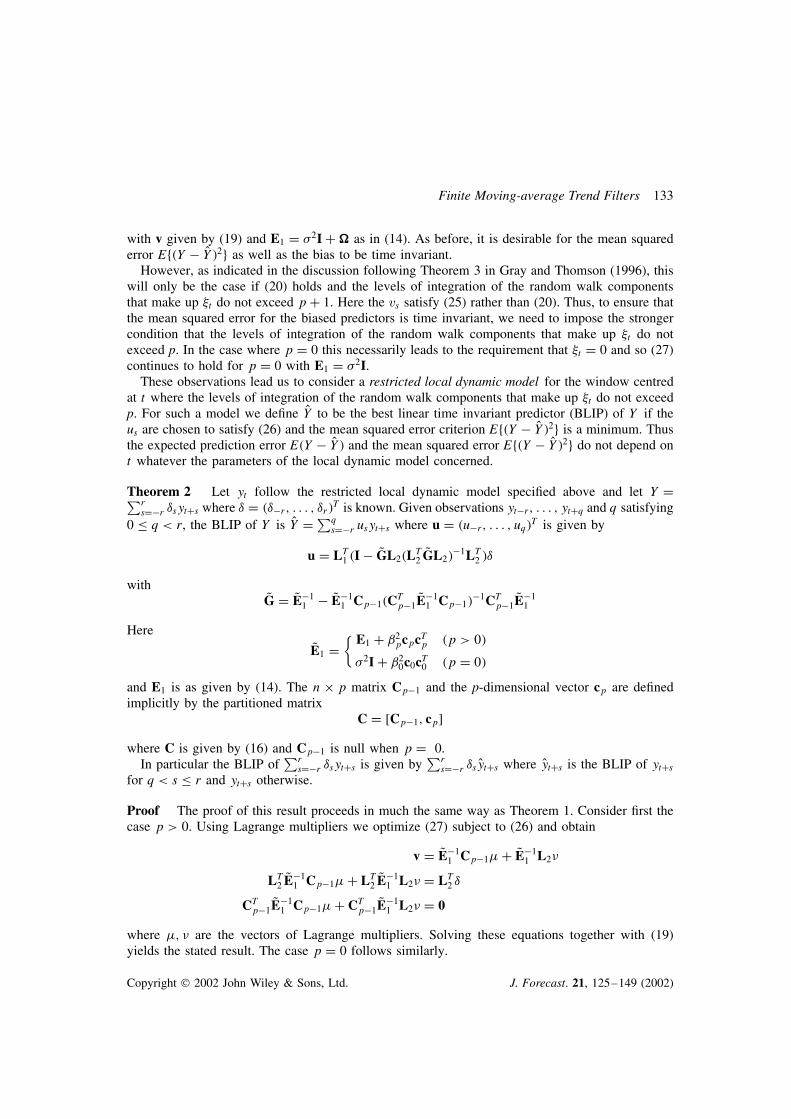
with v given by (19) and E1 D 2I CZ as in (14). As before, it is desirable for the mean squarederror Ef�Y� OY�2g as well as the bias to be time invariant.

However, as indicated in the discussion following Theorem 3 in Gray and Thomson (1996), thiswill only be the case if (20) holds and the levels of integration of the random walk componentsthat make up �t do not exceed pC 1. Here the vs satisfy (25) rather than (20). Thus, to ensure thatthe mean squared error for the biased predictors is time invariant, we need to impose the strongercondition that the levels of integration of the random walk components that make up �t do notexceed p. In the case where p D 0 this necessarily leads to the requirement that �t D 0 and so (27)continues to hold for p D 0 with E1 D 2I.

These observations lead us to consider a restricted local dynamic model for the window centredat t where the levels of integration of the random walk components that make up �t do not exceedp. For such a model we define OY to be the best linear time invariant predictor (BLIP) of Y if theus are chosen to satisfy (26) and the mean squared error criterion Ef�Y� OY�2g is a minimum. Thusthe expected prediction error E�Y� OY� and the mean squared error Ef�Y� OY�2g do not depend ont whatever the parameters of the local dynamic model concerned.

Theorem 2 Let yt follow the restricted local dynamic model specified above and let Y D∑rsD�r υsytCs where υ D �υ�r, . . . , υr�T is known. Given observations yt�r, . . . , ytCq and q satisfying

0 � q < r, the BLIP of Y is OY D ∑qsD�r usytCs where u D �u�r, . . . , uq�T is given by

u D LT1 �I � QGL2�LT2 QGL2��1LT2 �υ

withQG D QE�1

1 � QE�11 Cp�1�CTp�1

QE�11 Cp�1�

�1CTp�1QE�1

1

HereQE1 D

{ E1 C ˇ2pcpcTp �p > 0�

2I C ˇ20c0cT0 �p D 0�

and E1 is as given by (14). The nð p matrix Cp�1 and the p-dimensional vector cp are definedimplicitly by the partitioned matrix

C D [Cp�1, cp]

where C is given by (16) and Cp�1 is null when p D 0.In particular the BLIP of

∑rsD�r υsytCs is given by

∑rsD�r υs OytCs where OytCs is the BLIP of ytCs

for q < s � r and ytCs otherwise.

Proof The proof of this result proceeds in much the same way as Theorem 1. Consider first thecase p > 0. Using Lagrange multipliers we optimize (27) subject to (26) and obtain

v D QE�11 Cp�1!C QE�1

1 L2"

LT2 QE�11 Cp�1!C LT2 QE�1

1 L2" D LT2 υ

CTp�1QE�1

1 Cp�1!C CTp�1QE�1

1 L2" D 0

where !, " are the vectors of Lagrange multipliers. Solving these equations together with (19)yields the stated result. The case p D 0 follows similarly.



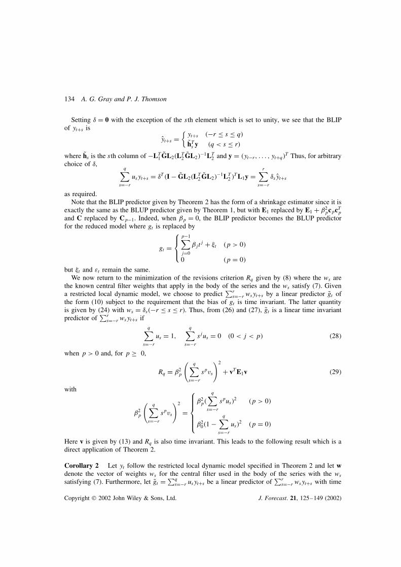
Setting υ D 0 with the exception of the sth element which is set to unity, we see that the BLIPof ytCs is

OytCs D{ytCs ��r � s � q�QhTs y �q < s � r�

where Qhs is the sth column of �LT1 QGL2�LT2 QGL2��1LT2 and y D �yt�r, . . . , ytCq�T Thus, for arbitrarychoice of υ,

q∑sD�r

usytCs D υT�I � QGL2�LT2 QGL2��1LT2 �

TL1y Dr∑

sD�rυs OytCs

as required.Note that the BLIP predictor given by Theorem 2 has the form of a shrinkage estimator since it is

exactly the same as the BLUP predictor given by Theorem 1, but with E1 replaced by E1 C ˇ2pcpcTp

and C replaced by Cp�1. Indeed, when ˇp D 0, the BLIP predictor becomes the BLUP predictorfor the reduced model where gt is replaced by

gt D

p�1∑jD0

ˇjtj C �t �p > 0�

0 �p D 0�

but �t and εt remain the same.We now return to the minimization of the revisions criterion Rq given by (8) where the ws are

the known central filter weights that apply in the body of the series and the ws satisfy (7). Givena restricted local dynamic model, we choose to predict

∑rsD�r wsytCs by a linear predictor Qgt of

the form (10) subject to the requirement that the bias of gt is time invariant. The latter quantityis given by (24) with ws D υs��r � s � r�. Thus, from (26) and (27), Qgt is a linear time invariantpredictor of

∑rsD�r wsytCs if

q∑sD�r

us D 1,q∑

sD�rsjus D 0 �0 < j < p� �28�

when p > 0 and, for p ½ 0,

Rq D ˇ2p

(q∑

sD�rspvs

)2

C vTE1v �29�

with

ˇ2p

(q∑

sD�rspvs

)2

D

ˇ2p�

q∑sD�r

spus�2 �p > 0�

ˇ20�1 �

q∑sD�r

us�2 �p D 0�

Here v is given by (13) and Rq is also time invariant. This leads to the following result which is adirect application of Theorem 2.

Corollary 2 Let yt follow the restricted local dynamic model specified in Theorem 2 and let wdenote the vector of weights ws for the central filter used in the body of the series with the wssatisfying (7). Furthermore, let Qgt D ∑q

sD�r usytCs be a linear predictor of∑rsD�r wsytCs with time



invariant bias so that the us satisfy (28). Then, for 0 � q < r, the values of us that minimize Rqsubject to (28) are given by Theorem 2 with υ D w and

q∑sD�r

usytCs Dr∑

sD�rws OytCs

Here OytCs is the BLIP of ytCs for q < s � r and ytCs otherwise.Because of their dependence on BLIP predictors we shall henceforth refer to the end filters

specified by Corollary 2 as BLIP end filters. Their properties are investigated in the next section.Now E1/ 2 does not depend on 2 and QE1 need only be known up to a constant of proportionality.

Thus, unlike the BLUP end filters specified by Corollary 1, the BLIP end filters specified byCorollary 2 can only be made operational when ˇ2

p/ 2 is known. Since this will rarely, if ever, be

the case, estimates of ˇ2p/

2 of one form or another need to be determined from the data. Suchestimates will, necessarily, differ from their true values and it is therefore important to determinethe effects of mis-specification of ˇ2

p/ 2. This issue is addressed below in Theorem 3 and also

in the following section where the properties of these end filters and the estimation of ˇ2p/

2 arediscussed.

Note that Corollary 2 yields the X-11 end filters derived by Musgrave (1964) and Doherty (1991)when �t D 0, p D 1, ˇ2

p/ 2 D 4/�%�3.5�2� and w contains the Henderson central filter weights. (See,

for example Henderson, 1924 and the alternative derivations given in e.g. Kenny and Durbin, 1982;Gray and Thomson, 1996.) Thus Corollary 2 provides a generalization and extension of the currentX-11 end filters.

The following result considers an alternative form of the BLIP end filters given by Corollary 2which explicitly builds on the corresponding BLUP end filters given by Corollary 1. In additionthe result provides a means of exploring the effects of mis-specification of ˇ2

p/ 2.

Theorem 3 Let yt follow the restricted local dynamic model specified in Theorem 2 and let wdenote the vector of weights ws for the central filter used in the body of the series with the ws satis-fying (7). Given observations yt�r, . . . , ytCq and q satisfying 0 � q < r, let Qgt D ∑q

sD�r us�&�ytCsbe a linear predictor of

∑rsD�r wsytCs where u�&� D �u�r�&�, . . . , uq�&��T is defined for every scalar

& byu�&� D LT1 �I − GL2�LT2 GL2�

�1LT2 ��w C &'�and

' D E�11 C�CTE�1

1 C��1d

Here L1,L2,G, E1 and C are as given in (17), Theorem 1, (14) and (16) respectively, and thepC 1-dimensional vector d is zero save for the last element which is unity. Then

(a) Qgt�&� is a linear time invariant predictor of∑rsD�r wsytCs with squared bias ˇ2

p&2 and the us�&�

satisfy (28) when p > 0;(b) The revisions criterion Rq is given in this case by

Rq�&� D wTHw C 2&'THw C &2�ˇ2p C dT�CTE�1

1 C��1d C 'TH'�

whereH D L2�LT2 GL2�

�1LT2



(c) The optimal end filters of Corollary 1 and Corollary 2 are given by u(0) and u�&0� respectivelywhere

&0 D � 'THw

ˇ2p C dT�CTE�1

1 C��1d C 'TH'

minimizes Rq�&�.

Proof First observe from Theorem 1 that Qgt�&� is the BLUP of∑rsD�r�ws C &'s�ytCs and CT' D

d so thatq∑

sD�rsp's D 1,

q∑sD�r

sj's D 0 �0 � j < p�

Thus, from (18),q∑

sD�rsjus�&� D

r∑sD�r

sj�ws C &'s� D{ 1 �j D 0�

0 �0 < j < p�& �j D p�

when p > 0 and∑qsD�r us�&� D 1 C & when p D 0. Moreover

E

{r∑

sD�rwsytCs � Qgt�&�

}D �&

r∑sD�r

'sE�ytCs� D �&ˇp

since CT' D d. This establishes (a).Now, from (29) and (13),

Rq�&� D ˇ2p&

2 C vTE1v

wherev D w � L1u�&�

Noting that LT2 �I � GH� D 0 we can write v as

v D w � �I � GH��w C &'�D GHw � &�I � GH�' �30�

and Rq�&� becomes

Rq�&� D wTHGE1GHw � 2&'T�I � HG�E1GHw

C &2�ˇ2p C 'T�I � HG�E1�I � GH�'T� �31�

Since GE1G D G, HGH D H and 'TE1G D 0, the above now reduces to the expression for Rq�&�given by (b).

From the form of u�&� it follows directly that u(0) is the optimal end filter given by Corollary 1.All that remains to prove is that u�&0� is the optimal end filter given by Corollary 2. Consideragain minimizing (29) with respect to the us where now v is defined by (13) and the us satisfy (28)if p > 0. This is equivalent to optimizing

QRq D ˇ2p&

2 C vTE1v � 2!T�CTv C &d�� 2"TLT2 �v � w�



with respect to v, & and the Lagrange multipliers !, ". Here & is a function of v defined by

& D �r∑

sD�rspvs D

q∑sD�r

spus �p > 0�

q∑sD�r

us � 1 �p D 0�

�32�

where the latter equality follows from (7) and (13). Optimizing QRq first with respect to v, µ and "we obtain the equations

v D E�11 C!C E�1

1 L2"

LT2 E�11 C!C LT2 E�1

1 L2" D LT2 w

CTE�11 C!C CTE�1

1 L2" D �&d

and these, together with (13), yield u D u�&�. Substituting this solution back into QRq gives Rq�&�which must now be optimized with respect to &. Since Rq�&� is a quadratic in & and takes itsminimum value when & D &0 result (c) follows.

An immediate consequence of Theorem 3 is that end filters based on BLIP predictors will gener-ally have smaller mean squared revisions than those based on the corresponding BLUP predictorssince Rq�&0� � Rq�0�. Moreover

Rq�&0� D wTHw � �'THw�2

ˇ2p C dT�CTE�1

1 C��1d C 'TH'

D Rq�0�� j&0jj'THwjso that Rq�&0� is a monotonically increasing function of ˇ2

p/ 2 and a linearly decreasing function

in j&0j. In particularlim

ˇ2p/

2!1Rq�&0� D Rq�0�, lim

ˇ2p/

2!1&0 D 0

so that BLIP end filters converge to their corresponding BLUP end filters as ˇ2p/

2 increases. Thebest possible mean squared revisions are achieved when ˇ2

p/ 2 D 0. Then Rq�&0� is least and, as

noted following Theorem 2, the BLIP end filters become BLUP end filters for the local dynamicmodel with order p� 1, but the same stochastic structure.

From the representation (30) and the properties of G and H , observe in passing that

cov

{r∑

sD�rwsytCs � Qgt�0�,

r∑sD�r

wsytCs � Qgt�&0�

}D wTHw C &0'

THw D Rq�&0�

so that the normalized quantity

Rq�&0�

Rq�0�D 1 � j&0j j'

THwjwTHw

represents the regression coefficient of the BLIP revisions∑rsD�r wsytCs � Qgt�&0� on the BLUP

revisions∑rsD�r wsytCs � Qgt�0�. Moreover, as noted in the proof to Theorem 3, Qgt�&� is the BLUP



of∑rsD�r wsytCs C &∑r

sD�r 'sytCs. Here∑rsD�r 'sytCs is the best linear unbiased estimator (BLUE)

of ˇp given yt�r, . . . , ytCr .Both the BLIP and BLUP end filters are dependent on the global parameters specified by p, n

and the model for �t/ . Although these global parameters are sufficient to determine the BLUPend filters, the BLIP end filters further require knowledge of ˇ2

p/ 2. The latter is a function of

local parameters whose values will not normally be known in practice and which will need to beestimated from the data. In this case it is possible that a mis-specified value of ˇ2

p/ 2 could result

in a BLIP end filter which has greater mean squared revisions than its corresponding BLUP endfilter.

Now Qgt�&0� depends only on ˇ2p/

2 through &0 which is a one-to-one function of ˇ2p/

2. ThusTheorem 3 enables us to consider the effects of mis-specification of ˇ2

p/ 2. Let O&0 denote &0

evaluated at O 2p/ O 2, some estimated or target value of ˇ2

p/ 2. Then, since Rq�&� is a quadratic in

&, it is evident that Rq� O&0� � Rq�0� if and only if O&0 lies between 0 and 2&0. The BLIP end filterswill therefore have better mean squared revisions than their corresponding BLUP end filters when

ˇ2p

2< 2

O 2p

O 2C �dT�CTE�1

1 C��1d C 'TH'�/ 2 �33�

In particular, since Rq�&0 C &� D Rq�&0 � &�, it is sufficient to select O 2p/ O 2 so that O&0 is between

0 and &0 or, equivalently, O 2p/ O 2 ½ ˇ2

p/ 2. In practice this choice should lead to values for O 2

p/ O 2

that, if anything, over-estimate ˇ2p/

2 thus controlling the mis-specification error by shrinking theBLIP end filter towards its BLUP counterpart. Note that if O 2

p/ O 2 ½ ˇ2p/

2 then

Qgt� O&0� D(

1 �O&0

&0

)Qgt�0�C

O&0

&0Qgt�&0�

(0 �

O&0

&0� 1

)

so that Qgt� O&0� is a convex combination of the two optimal end filters.The properties of these end filters are investigated in the following section.

PROPERTIES OF THE FILTERS

This section considers the properties of the end filters specified by Corollary 1 and Corollary 2which are designed to minimize the expected mean squared revisions between the output of thesefilters and that of the central filters on which they are based. These end filters deal with a transitionproblem that ultimately disappears as the current time points are subsumed into the body of theseries. The minimum revisions criterion therefore provides a measure of the total cost of thistransition.

We restrict attention to the important case where the window is of length 13 with r D 6 and thecentral filter used in the body of the series is the central Henderson filter. This case is the defaultused in the X-11 or X-12-ARIMA seasonal adjustment programs. Furthermore, we focus on twoparticular local dynamic models likely to be used in practice. These are the local linear model�p D 1� given by (3) and the local quadratic model �p D 2� given by (4).

Three end filters are considered: the BLUP end filter (or BLIP end filter with O 2p/ O 2 D 1),

the BLIP end filter with O 2p/ O 2 D 4/�%�3.5�2� (this gives the X-11 end filter in the case where



p D 1 and � D 0), and the BLIP end filter with O 2p/ O 2 D 0. As noted in the discussion following

Theorem 3, the smallest value of Rq�&� is achieved when & D &0 and ˇ2p/

2 D O 2p/ O 2 D 0. Also,

if O 2p/ O 2 is chosen so that (33) is satisfied or O 2

p/ O 2 ½ ˇ2p/

2, then the largest value of Rq�&0� isRq�0� which is the minimum revisions value for the BLUP end filter. These values serve as usefulbounds for Rq� O&0�.

To provide a range of possible values of ˇ2p/

2 we briefly consider the so-called I/C ratio usedby X-11 to specify the length of the trend moving-average adopted. Here I and C are the respectiveaverages of the absolute values of the month to month changes in the (estimated) irregular εt andtrend gt. Thus the I/C ratio measures the importance of month-to-month changes in εt relativeto those in the trend gt. X-11 recommends that the central 9-point Henderson filter be used whenI/C < 1, the central 13-point Henderson trend filter when 1 � I/C < 3.5, and the central 23-point Henderson trend filter when I/C ½ 3.5. Following Musgrave (1964) and Doherty (1991) weconsider the local linear model and

I

CD EjεtjEjgtj �34�

which can be thought of as the population parameter that I/C is estimating. Under Gaussianassumptions

I

CD 2√

% Q 21

(8

(j Q 1jp�

)�8

(�j Q 1jp

�

)C√

2�

% Q 21

exp

(�

Q 21

2�

))�1

where Q 1 D ˇ1/ and 8�x� is the standard normal cumulative distribution function. Simple evalu-ations show that the values of ˇ2

p/ 2 for which 1 � I/C < 3.5 lie in [0, 4/%]. This is the interval

of values for ˇ2p/

2 that we choose to adopt.We now examine the mean squared revisions of the given end filters for ˇ2

p/ 2 in [0, 4/%]. Note

that it is sufficient to consider the extremes of this interval since, from Theorem 3, Rq�&� is linearlyincreasing in ˇ2

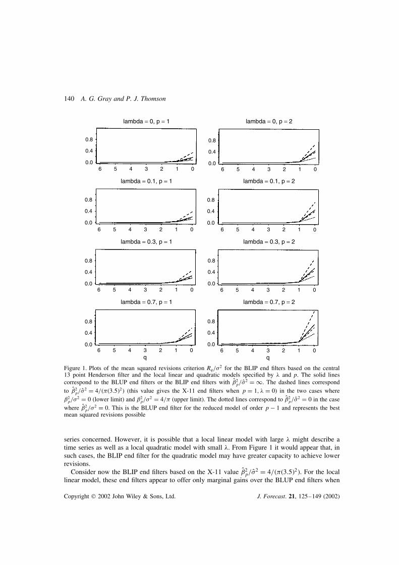
p over the interval for given &. The mean squared revisions criterion Rq� O&0�/ 2 isplotted in Figure 1 as a function of q for a selection of models and for the particular end filtersconsidered.

As expected, the mean squared revisions are greatest when q is least with q D 0 yielding thegreatest revisions followed by q D 1. The mean squared revisions for the other values of q arenegligible by comparison. Although not apparent on this scale, Rq� O&0�/ 2 is not necessarily amonotonic function of q. For example, the local quadratic model yields mean squared revisionswhen q D 2 that are typically smaller than those for q D 3. This is a consequence of the shape ofthe central Henderson filter adopted.

If O 2p/ O 2 has been selected appropriately, Rq� O&0�/ 2 will be bounded above by the mean squared

revisions for the BLUP end filter and below by the mean squared revisions for the BLIP end filterwith ˇ2

p/ 2 D O 2

p/ O 2 D 0. These bounds are plotted in Figure 1 and show that there are gains tobe had using BLIP end filters, although these are likely to be modest in the case of the local linearmodel. As evident from the form of Rq� O&0�/ 2 given by Theorem 3, the gains are greatest whenˇ2p/

2 is least.Note that the mean squared revisions generally increase as � and p increase. This is of marginal

utility in practice, since the local dynamic model chosen is determined from the particular time



6 5 4 3 2 1 0

6 5 4 3 2 1 0

6 5 4 3 2 1 0

6 5 4 3 2 1 0

0.0

0.4

0.8

0.0

0.4

0.8

0.0

0.4

0.8

0.0

0.4

0.8

lambda = 0.1, p = 1

lambda = 0.3, p = 1

lambda = 0.7, p = 1

q

lambda = 0, p = 1

6 5 4 3 2 1 0

6 5 4 3 2 1 0

6 5 4 3 2 1 0

6 5 4 3 2 1 0

0.0

0.4

0.8

0.0

0.4

0.8

0.0

0.4

0.8

0.0

0.4

0.8

lambda = 0.1, p = 2

lambda = 0.3, p = 2

lambda = 0.7, p = 2

q

lambda = 0, p = 2

Figure 1. Plots of the mean squared revisions criterion Rq/ 2 for the BLIP end filters based on the central13 point Henderson filter and the local linear and quadratic models specified by � and p. The solid linescorrespond to the BLUP end filters or the BLIP end filters with O 2

p/ O 2 D 1. The dashed lines correspondto O 2

p/ O 2 D 4/�%�3.5�2� (this value gives the X-11 end filters when p D 1, � D 0) in the two cases whereˇ2p/

2 D 0 (lower limit) and ˇ2p/

2 D 4/% (upper limit). The dotted lines correspond to O 2p/ O 2 D 0 in the case

where O 2p/

2 D 0. This is the BLUP end filter for the reduced model of order p� 1 and represents the bestmean squared revisions possible

series concerned. However, it is possible that a local linear model with large � might describe atime series as well as a local quadratic model with small �. From Figure 1 it would appear that, insuch cases, the BLIP end filter for the quadratic model may have greater capacity to achieve lowerrevisions.

Consider now the BLIP end filters based on the X-11 value O 2p/ O 2 D 4/�%�3.5�2�. For the local

linear model, these end filters appear to offer only marginal gains over the BLUP end filters when



ˇ2p/

2 satisfies (33). In the local quadratic case, they are clearly too conservative and a lower valueof O 2

p/ O 2 might more profitably be considered. For both models, the upper limit of ˇ2p/

2 D 4/%for these particular end filters lead to end filters with unacceptably high revisions. This may explain,in part, the reason why forecast extension using ARIMA models has largely superseded the useof the X-11 end filters in practice. The former yield (global) BLUP end filters with properties thatone might expect are close to the (local) BLUP end filters considered here. On the other hand,for the local linear model, the I/C guidelines imply that the X-11 end filters are inflexibly appliedwhenever ˇ2

p/ 2 satisfies ˇ2

p/ 2 � 4/% rather than (33).

It is of interest to consider the ranges of values of �j Opj/ O , jˇpj/ � that satisfy (33) and to ascertainthe general shape of Rq� O&0�/ 2 as a function of �jˇpj/ O , jˇpj/ � or, equivalently, � O 2

p/ O 2, ˇ2p/

2�.Plots of the lines

jˇpj

D√

2O 2p

O C �dT�CTE�11 C��1d C 'TH'�/ 2

are given in Figure 2 for q D 3, q D 0 and the local dynamic models (3) and (4) based on thecentral Henderson filter and selected values of �. From (33) the BLIP end filters have better meansquared revisions when �j Opj/ O , jˇpj/ � lies below the lines. For large values of j Opj/ O the BLIPend filters approach the BLUP end filters and the boundary becomes jˇpj/ D p

2j Opj/ O . However,for smaller values of j Opj/ O a somewhat greater range of possibilities is evident, especially for thelarger values of �. There is less latitude when p D 2 as might be expected. Given a range of (time-varying) values of jˇpj/ one would wish to select j Opj/ O as low as possible in order to maximizethe gains in terms of expected revisions.

Now consider Figure 3 which plots Rq� O&0�/Rq�0�, the mean squared revisions of the BLIPend filters normalized by the mean squared revisions of the BLUP end filters, as a function of�j Opj/ O , jˇpj/ �. Here only q D 0 is shown and the BLIP end filters are based on the local dynamicmodels (3) and (4), the central Henderson filter and selected values of �, jˇpj/ . Given j Opj/ O ,it follows from Theorem 3 that the normalized revisions Rq� O&0�/Rq�0� increase quadratically withincreasing jˇpj/ . From the plots and Theorem 3 a three-dimensional picture of Rq� O&0�/Rq�0� cannow be visualized. Looking out from the origin along the line jˇpj/ D j Opj/ O , Rq� O&0�/Rq�0� hasthe appearance of a rising valley with a sharply increasing left-hand side (representing the unac-ceptably high mean squared revisions incurred when �j Opj/ O , jˇpj/ � does not satisfy (33)) and aright-hand side that levels out at the BLUP limit Rq�0�/Rq�0� D 1. Note that the optimum meansquared revisions Rq�&0�/Rq�0� occur when jˇpj/ D j Opj/ O and, as noted in the discussion fol-lowing Theorem 3, Rq�&0� is a monotonically increasing function of jˇpj/ . Clearly the greatestgains are to be had when ˇ2

p/ 2 and hence O 2

p/ O 2 are small.If the BLUP end filters yield results that are comparable to ARIMA forecast extension, then it

would appear that judiciously selected BLIP end filters may offer modest performance gains interms of improved revisions. However the price of this improvement is a better understanding ofthe time varying values of ˇ2

p/ 2.

PRACTICAL STUDY

The outcomes of a preliminary study on selected official time series where the end filters given byCorollary 1 and Corollary 2 were compared with X-11 end filters and ARIMA forecast extension



0.0 0.2 0.4 0.6 0.8 1.00.0

0.5

1.0

1.5

0.0 0.2 0.4 0.6 0.8 1.00.0

0.5

1.0

1.5

lambda = 0, p = 1

lambda = 0.1, p = 1

lambda = 0.3, p = 1

lambda = 0.7, p = 1

|bet

a|/s

igm

a|b

eta|

/sig

ma

|bet

a|/s

igm

a|b

eta|

/sig

ma

|betahat|/sigmahat

0.0 0.2 0.4 0.6 0.8 1.00.0

0.5

1.0

1.5

0.0 0.2 0.4 0.6 0.8 1.00.0

0.5

1.0

1.5

0.0 0.2 0.4 0.6 0.8 1.00.0

0.5

1.0

1.5

0.0 0.2 0.4 0.6 0.8 1.00.0

0.5

1.0

1.5

lambda = 0, p = 2

lambda = 0.1, p = 2

lambda = 0.3, p = 2

lambda = 0.7, p = 2

|betahat|/sigmahat

0.0 0.2 0.4 0.6 0.8 1.00.0

0.5

1.0

1.5

0.0 0.2 0.4 0.6 0.8 1.00.0

0.5

1.0

1.5

Figure 2. Plots of the lines in the �j Opj/ O , jˇpj/ � plane below which BLIP end filters have better mean squaredrevisions than BLUP end filters. Here the BLIP end filters are based on the central 13-point Henderson filter,and the local linear and quadratic models are specified by p and �. The solid lines correspond to q D 0,the dotted lines to q D 3 and the dashed line to the case jˇpj/ D j Opj/ O when the optimum revisions areachieved for a given value of jˇpj/ . The vertical dotted line is j Opj/ O D √

4/�%�3.5�2�, a value derived fromrecommendations made by X-11 concerning I/C ratios

were reported in Gray and Thomson (1996). In this section we shall discuss salient features fromthat study and illustrate how the theoretical properties mentioned in the previous section are realizedin practice.

Description of the time seriesAll the time series we examined were seasonal and some of them had large outliers. Since thetrend filters under study are for non-seasonal time series and have not yet been modified tohandle outliers, the first task in this analysis was to remove the seasonal component and large



0.0 0.2 0.4 0.6 0.8 1.00.4

0.8

1.2

0.0 0.2 0.4 0.6 0.8 1.00.4

0.8

1.2

0.0 0.2 0.4 0.6 0.8 1.00.4

0.8

1.2

0.0 0.2 0.4 0.6 0.8 1.00.4

0.8

1.2

0.0 0.2 0.4 0.6 0.8 1.00.4

0.8

1.2

0.0 0.2 0.4 0.6 0.8 1.00.4

0.8

1.2

0.0 0.2 0.4 0.6 0.8 1.00.4

0.8

1.2

0.0 0.2 0.4 0.6 0.8 1.00.4

0.8

1.2

lambda = 0, p = 1 lambda = 0, p = 2

lambda = 0.1, p = 2

lambda = 0.3, p = 2

lambda = 0.7, p = 2

lambda = 0.1, p = 1

lambda = 0.3, p = 1

lambda = 0.7, p = 1

|betahat|/sigmahat |betahat|/sigmahat

Figure 3. Plots of Rq� O&0�/Rq�0�, the mean squared revisions of the BLIP end filters normalized by the meansquared revisions of the BLUP end filters, as a function of �j Opj/ O , jˇpj/ �. Here q D 0 and the BLIP endfilters are based on the local linear �p D 1� and quadratic �p D 2� models, the central 13 point Hendersonfilter and selected values of �, jˇpj/ . For given j Opj/ O the normalized revisions Rq� O&0�/Rq�0� increasequadratically with increasing jˇpj/ . The solid lines correspond to ˇ2

p/ 2 D 0 (this yields the best mean

squared revisions possible for any given value of ˇ2p/ O 2), the dotted lines to ˇ2

p/ 2 D 4/�%�3.5�2�, the dashed

lines to ˇ2p/

2 D 4/% and the vertical dotted line to j Opj/ O D √4/�%�3.5�2�. These values are derived from

recommendations made by X-11 concerning I/C ratios

outliers from the time series so that we could examine the relative performance of these filters.For simplicity we used the modified seasonally adjusted series from the X-11 seasonal adjust-ment method as the data for this study. We chose a window of the series which we believedwould give a good X-11 decomposition. Other than choosing the commonly used limits of 1.8and 2.8 for treating outliers we used the default options of X-11 to produce the seasonallyadjusted data.



The resulting non-seasonal times series presented different types of short- and long-term trendsand their local dynamic models included random walk components with a range of variances. Inthis section we shall discuss three monthly series representing this range of trend behaviour. Theseare as follows.

ž Building Permits New Zealand data from January 1985 to December 1992 on the number ofBuilding Permits issued by Local Authorities for the construction of private houses and flats.This subset of the data was chosen in order to get a consistent series where, for example, therewas no Government intervention in Housing Policy.

ž Merchandise Exports New Zealand data from January 1986 to December 1992 on the valueof Merchandise Exports. This subset of the data was chosen in order to get a consistent serieswhere the economy had adjusted to the impact of deregulation in the mid-1980s.

ž Permanent Migration New Zealand data on the Net Permanent and Long Term Migration fromJanuary 1982 to December 1992.

Fitting the local dynamic modelRecall that the parameters of the local dynamic model are the window length n D 2r C 1, the orderof the polynomial p, and a value of �. To study the filters based on the local dynamic model allthese parameters must be determined from the data, although to some extent the choice of n willbe be influenced by the overall objectives of the smoothing.

Typically n and p are identified from a simple graphical analysis of the data although more formalmethods could be used. Given n and p, there are a variety of methods for determining �. Theserange from trial and error and simple variational arguments based on quantities like X-11’s I/Cratio through to likelihood analysis based on fitting the local dynamic model within non-overlappingwindows, etc. Which approach turns out to be most useful is still very much an open question andthe subject of further research. Here we adopted a simple and direct method of estimating � thattook advantage of the unbiased BLUP predictors.

Consider the family of BLUP end filters based on Corollary 1 for a given central filter and givenvalues of n and p. Note that since these end filters are unbiased they depend only on q and �.Applying the end filters to the data yields the revisions

rt�q, �� Dr∑

�rwsytCs �

q∑�rus��ytCs

where the ws are the given central filter weights and the us�� are the BLUP end filter weightsgiven by Corollary 1. An appropriate cost function such as

P Dr�1∑qD0

˛qr2t �q, �� 35�

can now be constructed with the given positive weights ˛q reflecting the relative costs of therespective revisions. Finally � is determined by minimizing P with respect to �.

For our study n D 13, p D 1 and the central filter chosen was the central Henderson filter.Moreover we chose ˛0 D 1 and ˛q D 0 for q 6D 0 yielding a cost function which focused on thecase of worst revisions. However, other central filters and other values for the ˛q could have beenchosen and would lead to different results. Again, more research is needed, but it is believed that the



results presented here are indicative of what might be achieved more generally. With these caveats,this procedure was applied to Building Permits, Exports and Permanent Migration, yielding valuesfor � of 0.046, 0.52, and 3.8 respectively.

Finally we consider the estimation of the ratio jˇpj/ which involves the local parameters ˇpand . Although local estimates of jˇpj/ should be explored in order to minimize revisions fromBLIP end filters, this option was left for further study. Instead we adopted the more conservativestrategy of estimating a common value for jˇpj/ for each of the series considered.

To determine a global value for j Opj/ O from the data we adopted a similar approach to thatused for determining �, but now focused on the BLIP end filters given by Corollary 2. Here wedetermined the revisions

Qrt�q, j Opj/ O � Dr∑

�rwsytCs �

q∑�rus�j Opj/ O �ytCs

where the ws are the known central filter weights, the us�j Opj/ O � are the BLIP end filter weightsgiven by Corollary 2 and n, p are given. The value of � is set at its previously estimated value.Now the cost function QP given by (35) with rt replaced by Qrt can be evaluated and minimized withrespect to j Opj/ O .

As before, we chose ˛0 D 1, ˛q D 0 for q 6D 0 and set n D 13, p D 1 with the central filterchosen to be the central Henderson filter. Minimizing QP in this way for Building Permits, Exportsand Permanent Migration, yielded global values for j Opj/ O of 0.22, 0.3, and 0.32 respectively. Bycontrast, the X-11 value for j Opj/ O is 0.322. As was noted before in relation to the estimation of �,different central filters and different values of ˛q could have been chosen and would give differentresults.

Comparative performanceIn this subsection we consider the comparative performance of the BLIP, BLUP, X-11 and ARIMAforecast extension filters on the data sets under study. Here, as before, the window length isn D 13 and only the local linear model �p D 1� is considered with � and a global value for j Opj/ O determined by the methods described in the previous subsection. As mentioned in that section, amore appropriate procedure would have been to determine local values for j Opj/ O and use these inthe BLIP end filters. However this was not done and remains a topic for further research. It mightbe expected that the use of local values for j Opj/ O would lead to BLIP end filters with improvedperformance over those using a global value for j Opj/ O .

The following empirical comparison of the competing end filters was undertaken. First, for eachlocal window we calculated the trend for the central point of that window using the central filter(5). Next, for each q and for each local window, we calculated the trend using the appropriateend filter. For the BLUP and BLIP cases, this meant predicting the trend as in (10), where theys are the weights of the end filter determined by Corollaries 1 and 2 respectively. For the X-11case the standard X-11 end filters were applied. Recall that these are given by Corollary 2 usingthe central Henderson filter, O 2

p/ O 2 D 4/�%�3.5�2� and the local linear model with � D 0. For theARIMA forecast extension case this meant predicting the trend as in (9) with ytCs now predictedusing a global ARIMA model fitted to all the data available up to and within the local window.Finally, for each of these methods, the differences between the central filter trend estimates andthe end filter trend estimates were calculated to give the revisions which occur as predictions of



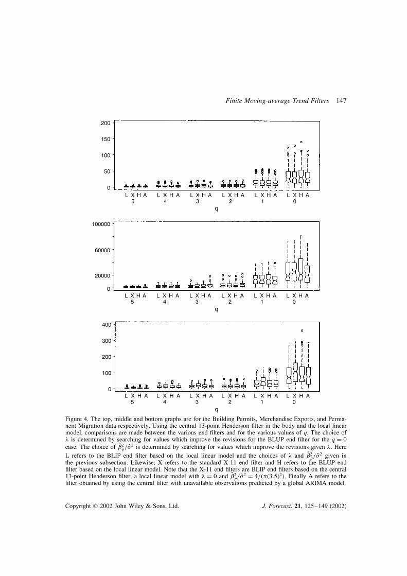
missing data are replaced by their actual values. Boxplots of the absolute value of the revisions aregiven in Figure 4.

Further comments about the ARIMA forecast extension case are in order. We note that theresulting end filter is essentially that proposed in Dagum (1996) and, by contrast to the BLIPand BLUP end filters which use only observations within the local window, the ARIMA forecastextension end filter involves the available observations within the window and, in principle, allprevious observations as well. To obtain appropriate ARIMA model parameters we fitted globalARIMA models to all the data. This was done for reasons of simplicity and to provide stableestimates. However, it puts our procedure at a disadvantage since the ARIMA global models aretaking advantage of future values, which is not possible in practice. Using the AIC criterion andother standard diagnostics we selected ARIMA (0,1,1) models for Building Permits and PermanentMigration, and an ARIMA (2,1,0) model for Exports. Other global predictive models could havebeen chosen instead of ARIMA models including structural unobserved component models suchas those given in Harvey (1989). However, this has not been investigated, in part because theseparticular models are a subset of the more general ARIMA model class considered here.

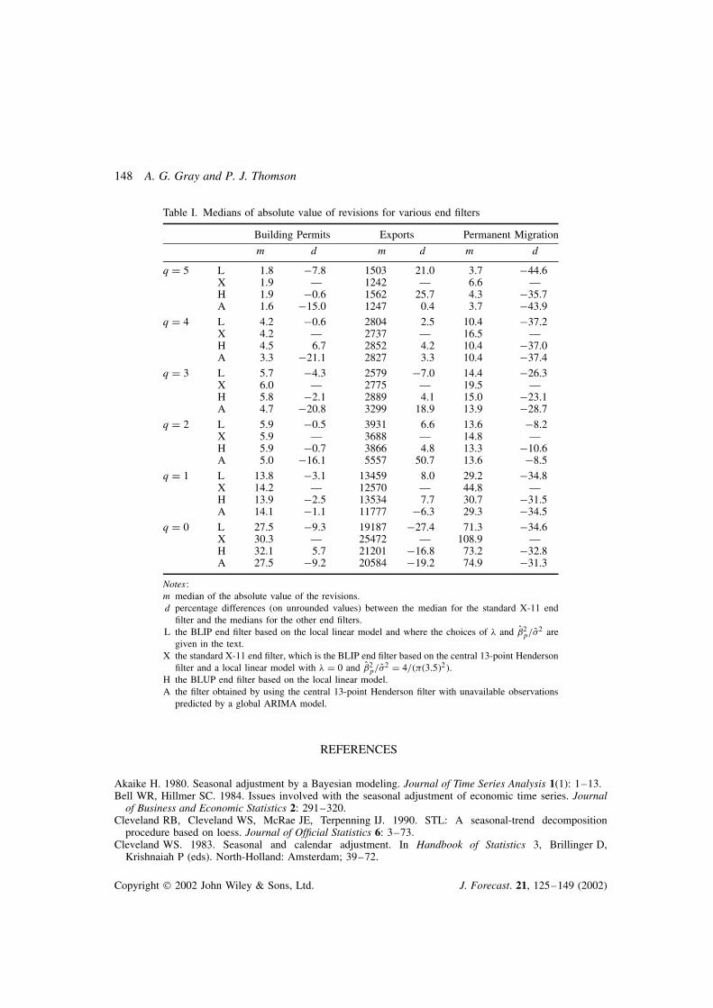
In accord with the discussion of the theoretical properties of these filters, Figure 4 shows thatthe greatest revisions and spread of revisions occurred when q D 0 followed by q D 1. It is notclear in making comparisons whether one should focus on the median or the lower quartile of thedistribution of the revisions, or the upper quartile or the interquartile range, or even the outliers.Depending on the cost function associated with revisions, a case can be made for each of these.Here we focus on the median because that provides a robust estimate of the square root of the meansquared revisions (up to a scale factor). The mean squared revisions criterion was used to evaluatethe theoretical performance of the filters in the previous section. To further assist comparison,Table I provides the values of the medians for each of the series for the various values of q.

As expected from Theorem 3, the BLIP end filters where j Opj/ O is determined from the datagenerally have smaller revisions than BLUP end filters and smaller revisions than the Musgraveend filters used in X-11. (These are BLIP end filters based on the central Henderson filter, a locallinear model with � D 0 and O 2

p/ O 2 set to 4/�%�3.5�2�.) For the Exports and Permanent Migrationseries, although the choice of j Opj/ O is similar to the X-11 value, the value of � used in the X-11end filters is inappropriate and so here, in the main, the X-11 end filters have larger revisions thanthe BLUP end filters. For all cases when q D 0 and for Building permits and Permanent Migrationwhen q D 1, the BLIP end filter with j Opj/ O determined from the data performed at least as wellas if not better than ARIMA forecast extension.

The results presented in this section are indicative and promising. A larger study is being plannedto validate these results more generally. In particular the study will also check whether furtherimprovement can be achieved by using local (adaptive) estimates of j Opj/ O .

ACKNOWLEDGEMENTS

The second author gratefully acknowledges support provided by an ASA/NSF/Census ResearchFellowship which he held at the US Bureau of the Census. In particular, both authors wish to recordtheir gratitude to Dr David Findley of that organization for the helpful advice and encouragementhe has provided throughout the project. The data was kindly provided by Statistics New Zealandand the authors are grateful to the referees and the editor for suggesting a number of improvements.



L X H A L X H A L X H A L X H A L X H A L X H A5 4 3 2 1 0

q


q


q

0

50

100

150

200

0

0

100

200

300

400

20000

60000

100000

Figure 4. The top, middle and bottom graphs are for the Building Permits, Merchandise Exports, and Perma-nent Migration data respectively. Using the central 13-point Henderson filter in the body and the local linearmodel, comparisons are made between the various end filters and for the various values of q. The choice of� is determined by searching for values which improve the revisions for the BLUP end filter for the q D 0case. The choice of O 2

p/ O 2 is determined by searching for values which improve the revisions given �. HereL refers to the BLIP end filter based on the local linear model and the choices of � and O 2

p/ O 2 given inthe previous subsection. Likewise, X refers to the standard X-11 end filter and H refers to the BLUP endfilter based on the local linear model. Note that the X-11 end filters are BLIP end filters based on the central13-point Henderson filter, a local linear model with � D 0 and O 2

p/ O 2 D 4/�%�3.5�2�. Finally A refers to thefilter obtained by using the central filter with unavailable observations predicted by a global ARIMA model



Table I. Medians of absolute value of revisions for various end filters

Building Permits Exports Permanent Migration

m d m d m d

q D 5 L 1.8 �7.8 1503 21.0 3.7 �44.6X 1.9 — 1242 — 6.6 —H 1.9 �0.6 1562 25.7 4.3 �35.7A 1.6 �15.0 1247 0.4 3.7 �43.9

q D 4 L 4.2 �0.6 2804 2.5 10.4 �37.2X 4.2 — 2737 — 16.5 —H 4.5 6.7 2852 4.2 10.4 �37.0A 3.3 �21.1 2827 3.3 10.4 �37.4

q D 3 L 5.7 �4.3 2579 �7.0 14.4 �26.3X 6.0 — 2775 — 19.5 —H 5.8 �2.1 2889 4.1 15.0 �23.1A 4.7 �20.8 3299 18.9 13.9 �28.7

q D 2 L 5.9 �0.5 3931 6.6 13.6 �8.2X 5.9 — 3688 — 14.8 —H 5.9 �0.7 3866 4.8 13.3 �10.6A 5.0 �16.1 5557 50.7 13.6 �8.5

q D 1 L 13.8 �3.1 13459 8.0 29.2 �34.8X 14.2 — 12570 — 44.8 —H 13.9 �2.5 13534 7.7 30.7 �31.5A 14.1 �1.1 11777 �6.3 29.3 �34.5

q D 0 L 27.5 �9.3 19187 �27.4 71.3 �34.6X 30.3 — 25472 — 108.9 —H 32.1 5.7 21201 �16.8 73.2 �32.8A 27.5 �9.2 20584 �19.2 74.9 �31.3

Notes:m median of the absolute value of the revisions.d percentage differences (on unrounded values) between the median for the standard X-11 end

filter and the medians for the other end filters.L the BLIP end filter based on the local linear model and where the choices of � and O 2

p/ O 2 aregiven in the text.

X the standard X-11 end filter, which is the BLIP end filter based on the central 13-point Hendersonfilter and a local linear model with � D 0 and O 2

p/ O 2 D 4/�%�3.5�2�.H the BLUP end filter based on the local linear model.A the filter obtained by using the central 13-point Henderson filter with unavailable observations

predicted by a global ARIMA model.

REFERENCES

Akaike H. 1980. Seasonal adjustment by a Bayesian modeling. Journal of Time Series Analysis 1(1): 1–13.Bell WR, Hillmer SC. 1984. Issues involved with the seasonal adjustment of economic time series. Journal

of Business and Economic Statistics 2: 291–320.Cleveland RB, Cleveland WS, McRae JE, Terpenning IJ. 1990. STL: A seasonal-trend decomposition

procedure based on loess. Journal of Official Statistics 6: 3–73.Cleveland WS. 1983. Seasonal and calendar adjustment. In Handbook of Statistics 3, Brillinger D,

Krishnaiah P (eds). North-Holland: Amsterdam; 39–72.



Cleveland WS, Dunn DM, Terpenning IJ. 1978. SABL—A resistant seasonal adjustment procedure withgraphical methods for interpretation and diagnosis. In Seasonal Analysis of Economic Time Series, Zellner A(ed). U S Department of Commerce, US Bureau of the Census: Washington, DC; 201–231.

Dagum EB. 1980. The X-11-ARIMA seasonal adjustment method. Research paper, Statistics Canada, OttawaK1A 0T6.

Dagum EB. 1996. A new method to reduce unwanted ripples and revisions in trend-cycle estimates fromX11ARIMA. Survey Methodology 22(1): 77–83.

DeForest EL. 1877. On adjustment formulas. The Analyst 4: 79–86, 107–113.Doherty M. 1991. Surrogate Henderson filters in X-11. Technical report, NZ Department of Statistics,

Wellington, New Zealand.Findley DF, Monsell BC, Bell WR, Otto MC, Chen B-C. 1998. New capabilities and methods of the X-12-

ARIMA seasonal-adjustment program. Journal of Business and Economic Statistics 16(2): 27–177.Gersch W, Kitagawa G. 1983. The prediction of time series with trends and seasonalities. Journal of Business

and Economic Statistics 1: 253–264.Geweke J. 1978. The revision of seasonally adjusted time series. In Proceedings of the Business and Economic

Statistics Section, American Statistical Association, 320–325.Gray AG Thomson P. 1996. Design of moving-average trend filters using fidelity, smoothness and minimum

revisions criteria. Research Report CENSUS/SRD/RR-96/1, Statistical Research Division, Bureau of theCensus, Washington, DC 20233–4200.

Greville TNE. 1979. Moving-weighted-average smoothing extended to the extremities of the data. TechnicalSummary Report #2025, Mathematics Research Center, University of Wisconsin, Madison, Wisconsin.

Harvey AC. 1989. Forecasting, Structural Time Series Models and the Kalman Filter. Cambridge UniversityPress: Cambridge.

Henderson R. 1924. A new method of graduation. Transactions of the Actuarial Society of America 25: 29–40.Hillmer SC, Tiao GC. 1982. An ARIMA model based approach to seasonal adjustment. Journal of the

American Statistical Association 77: 63–70.Kenny PB, Durbin J. 1982. Local trend estimation and seasonal adjustment of economic and social time series.

Journal of the Royal Statistical Society, Series A 145: 1–41.Lane ROD. 1972. Minimal revision trend estimates. Technical Report Research Exercise Note 8/72, Central

Statistical Office, London.Laniel N. 1986. Design criteria for 13 term Henderson end-weights. Technical Report Working Paper TSRA-

86-011, Statistics Canada, Ottawa K1A 0T6.Maravall A. 1993. Stochastic linear trends, models and estimators. Journal of Econometrics 56: 5–37.Musgrave J-C. 1964. A set of end weights to end all end weights. Working paper, Bureau of the Census, US

Department of Commerce, Washington, DC.Pierce DA. 1980. Data revisions with moving average seasonal adjustment procedures. Journal of

Econometrics 14: 95–114.Schlicht E. 1981. A seasonal adjustment principle and a seasonal adjustment method derived from this

principle. Journal of the American Statistical Association 76: 374–378.Wallis KF. 1983. Models for X-11 and X-11-FORECAST procedures for preliminary and revised seasonal

adjustments. In Applied Time Series Analysis of Economic Data, Zellner A (ed.). US Bureau of the Census:Washington, DC; 3–11.

Young PC, Pedregal D, Tych W. 1999. Dynamic harmonic regression (DHR). Journal of Forecasting 18:369–394.

Authors’ addresses:Alistair G. Gray, Statistics New Zealand, PO Box 2922, Wellington, New Zealand.

Peter J. Thomson, Statistics Research Associates Ltd, PO Box 12649, Thorndon, Wellington, New Zealand.


On a family of finite moving-average trend filters for the ...

Documents

Transcript of On a family of finite moving-average trend filters for the ...