OMPUT c - Massachusetts Institute of Technology

Copyright © by SIAM. Unauthorized reproduction of this article is prohibited.

SIAM J. SCI. COMPUT. c© 2009 Society for Industrial and Applied MathematicsVol. 31, No. 4, pp. 2549–2567

MINIMAL REPETITION DYNAMIC CHECKPOINTINGALGORITHM FOR UNSTEADY ADJOINT CALCULATION∗

QIQI WANG† , PARVIZ MOIN† , AND GIANLUCA IACCARINO†

Abstract. Adjoint equations of differential equations have seen widespread applications inoptimization, inverse problems, and uncertainty quantification. A major challenge in solving adjointequations for time dependent systems has been the need to use the solution of the original systemin the adjoint calculation and the associated memory requirement. In applications where storing theentire solution history is impractical, checkpointing methods have frequently been used. However,traditional checkpointing algorithms such as revolve require a priori knowledge of the number oftime steps, making these methods incompatible with adaptive time stepping. We propose a dynamiccheckpointing algorithm applicable when the number of time steps is a priori unknown. Our algorithmmaintains a specified number of checkpoints on the fly as time integration proceeds for an arbitrarynumber of time steps. The resulting checkpoints at any snapshot during the time integration havethe optimal repetition number. The efficiency of our algorithm is demonstrated both analyticallyand experimentally in solving adjoint equations. This algorithm also has significant advantage inautomatic differentiation when the length of execution is variable.

Key words. adjoint equation, dynamic checkpointing, automatic differentiation, checkpointingscheme, optimal checkpointing, online checkpointing, revolve

AMS subject classifications. 68W05, 49J20, 65D25

DOI. 10.1137/080727890

1. Introduction. In numerical simulation of dynamical systems, the adjointequation is commonly used to obtain the derivative of a predefined objective functionwith respect to many independent variables that control the dynamical system. Thisapproach, known as the adjoint method, has many uses in scientific and engineeringsimulations. In control theory-based optimization problems and inverse problems,the derivative obtained via the adjoint method is used to drive a gradient-based op-timization iteration procedure [1], [10]. In posterior error estimation and uncertaintyquantification, this derivative is used to analyze the sensitivity of an objective func-tion to various uncertain parameters and conditions of the system [12], [3], [4]. Anefficient numerical solution of the adjoint equation is essential to these adjoint-basedapplications.

The main challenge in solving the adjoint equations for time dependent systemsresults from their time-reversal characteristic. Although a forward-time Monte Carloalgorithm [14] has been proposed for solving the adjoint equations, checkpointingschemes remain the dominant method to address this challenge. For a general non-linear dynamical system (referred to here as the original system as opposed to theadjoint system)

u̇ = G(u, t), u(0) = u0, 0 ≤ t ≤ T,

its adjoint equation is a linear dynamical system with a structure similar to theoriginal system, except that the adjoint equation is initialized at time T . It then

∗Received by the editors June 19, 2008; accepted for publication (in revised form) February 26,2009; published electronically June 19, 2009. This work supported by the United States Departmentof Energy’s ASC and PSAAP programs at Stanford University.

http://www.siam.org/journals/sisc/31-4/72789.html†Center for Turbulence Research, Stanford University, Stanford, CA 94305 ([email protected],

[email protected], [email protected]).

2549


2550 QIQI WANG, PARVIZ MOIN, AND GIANLUCA IACCARINO

evolves backward in time such that

q̇ = A(u, t)q + b(u, t), q(T ) = q0(u(T )), 0 ≤ t ≤ T.

While the specific forms of q0, A, and b depend on the predefined objective function,the required procedure to solve the adjoint equation is the same: To initialize theadjoint equation, u(T ) must first be obtained; as the time integration proceeds back-ward in time, the solution of the original system u is needed from t = T backward tot = 0. At each time step of the adjoint time integration, the solution of the originalsystem at that time step must be either already stored in memory or recalculatedfrom the solution at the last stored time step. If we have sufficient memory to storethe original system at all the time steps, the adjoint equation can be solved withoutrecalculating the original system. High fidelity scientific and engineering simulations,however, require both many time steps and large memory to store the solution ateach time step, making the storage of the solution at all the time steps impractical.Checkpointing schemes, in which only a small number of time steps is stored, applynaturally in this situation. Surprisingly, checkpointing does not necessarily take morecomputing time than storing all time steps, since the modified memory hierarchy maycompensate for the required recalculations [11].

Checkpointing schemes can significantly reduce the memory requirement but mayincrease the computation time [2], [7]. In the first solution of the original system, thesolutions at a small set of carefully chosen time steps called checkpoints are stored.During the following adjoint calculation, the discarded intermediate solutions arethen recalculated by solving the original system restarting from the checkpoints. Oldcheckpoints are discarded once they are no longer useful, while new checkpoints arecreated in the recalculation process and replace the old ones. Griewank [5] proposed abinomial checkpointing algorithm for certain values of the number of time steps. Thisrecursive algorithm, known as revolve, has been proven to minimize the number ofrecalculations for any given number of allowed checkpoints and all possible numberof time steps [6]. With s number of allowed checkpoints and t recalculations,

(s+t

t

)time steps can be integrated. The revolve algorithm achieves logarithmic growth ofspatial and temporal complexity with respect to the number of time steps, acceptablefor the majority of scientific and engineering simulations.

Griewank’s revolve algorithm assumes a priori knowledge of the number of timesteps, which represents an inconvenience, perhaps even a major obstacle in certain ap-plications. In solving hyperbolic partial differential equations, for example, the size ofeach time step Δt can be constrained by the maximum wavespeed in the solution field.As a result, the number of time steps taken for a specified period of time is not knownuntil the time integration is completed. A simple but inefficient workaround is to solvethe original system once for the sole purpose of determining the number of time steps,before applying the revolve algorithm. Two algorithms have been developed to gen-erate checkpoints with unknown number of time steps a priori. The first is a-revolve

[9]. For a fixed number of allowed checkpoints, the a-revolve algorithm maintainsa cost function that approximates the total computation time of recalculating allintermediate solutions based on current checkpoint allocation. As time integrationproceeds, the heuristic cost function is minimized by reallocating the checkpoints.Although a priori knowledge of the number of time steps is not required, the a-

revolve algorithm is shown to be only slightly more costly than Griewank’s revolve

algorithm. However, it is difficult to prove a theoretical bound with this algorithm,making its superiority to the simple workaround questionable. The other algorithm is


DYNAMIC CHECKPOINTING FOR UNSTEADY ADJOINT 2551

the online checkpointing algorithm [8]. This algorithm theoretically proves to beoptimal; however, it explicitly assumes that the number of time steps is no more than(s+2

s

)and produces an error when this assumption is violated. This upper bound in the

number of time steps is extended to(s+3

s

)in a recent work [13]. This limitation makes

their algorithm unsuitable for large number of time steps when the memory is limited.We propose a dynamic checkpointing algorithm for solving adjoint equations.

This algorithm, compared to previous ones, has three main advantages: First, unlikeGriewank’s revolve, it requires no a priori knowledge of the number of time steps andis applicable to both static and adaptive time stepping. Second, in contrast to Hinzeand Sternberg’s a-revolve, our algorithm is theoretically optimal in that it minimizesthe repetition number t, defined as the maximum number of times a specific time stepis evaluated during the adjoint computation. As a result, the computational cost hasa theoretical upper bound. Third, our algorithm works for an arbitrary number oftime steps, unlike previous online checkpointing algorithms which limit the length ofthe time integration. When the number of time steps is less than

(s+2

s

), our algorithm

produces the same set of checkpoints as Heuveline and Walther’s result; as the numberof time steps exceeds this limit, our algorithm continues to update the checkpoints andensures their optimality in the repetition number t. We prove that for arbitrarily largenumber of time steps, the maximum number of recalculations for a specific time stepin our algorithm is as small as possible. This new checkpointing algorithm combinesthe advantages of previous algorithms without having the drawbacks of them.

As with revolve, our dynamic checkpointing algorithm is applicable both insolving adjoint equations and in reverse mode automatic differentiation (AD). re-

volve and other static checkpointing algorithms can be inefficient in differentiatingcertain types of source code whose length of execution is a priori uncertain. Exam-ples include “while” statements where the number of loops to be executed is onlydetermined during execution and procedures with large chunks of code in “if” state-ments. These cases may seriously degrade the performance of static checkpointingAD schemes. Our dynamic checkpointing algorithm can solve this issue by achievingclose to optimal efficiency regardless of the length of execution. Since most sourcecodes to which automatic differentiation is applied are complex, our algorithm cansignificantly increase the overall performance of AD software.

This paper is organized as follows. In section 2 we first demonstrate our check-point generation algorithm. We prove the optimality of the algorithm, based on anassumption about the adjoint calculation procedure. Section 3 proves this assump-tion by introducing and analyzing our full algorithm for solving adjoint equations,including checkpoint-generation and checkpoint-based recalculations in backward ad-joint calculation. The performance of the algorithm is theoretically analyzed andexperimentally demonstrated in section 4. Conclusions are provided in section 5.

2. Dynamic checkpointing algorithm. The key concepts of time step index,level, and dispensability of a checkpoint must be defined before introducing our algo-rithm. The time step index is used to label the intermediate solutions of both theoriginal equation and the adjoint equation at each time step. It is 0 for the initialcondition of the original equation, 1 for the solution after the first time step, andincrements as the original equation proceeds forward. For the adjoint solution, thetime step index decrements and reaches 0 for the last time step of the adjoint timeintegration. The checkpoint with time step index i, or equivalently, the checkpointat time step i, is defined as the checkpoint that stores the intermediate solution withtime step index i.



Algorithm 1 Dynamic allocation of checkpoints.Require: s > 0 given.

Save time step 0 as a checkpoint of level ∞;for i = 0, 1, . . . do

if the number of checkpoints <= s thenSave time step i + 1 as a checkpoint of level 0;

else if at least one checkpoint is dispensable thenRemove the dispensable checkpoint with the largest time step index;Save time step i + 1 as a checkpoint of level 0;

elsel ⇐ the level of checkpoint at time step i;Remove the checkpoint at time step i;Save time step i + 1 as a checkpoint of level l + 1;

end ifCalculate time step i + 1 of the original system;

end for.

We define the concept of level and dispensability of checkpoints in our dynamiccheckpointing algorithm. As each checkpoint is created, a fixed level is assigned to it.We will prove in section 3 that this level indicates how many recalculations are neededto reconstruct all intermediate solutions between the checkpoint and the previouscheckpoint of the same level or higher. We define a checkpoint as dispensable if its timestep index is smaller than another checkpoint of a higher level. When a checkpoint iscreated, it has the highest time step index and is therefore not dispensable. As newcheckpoints are added, existing checkpoints become dispensable if a new checkpointhas a higher level. Our algorithm allocates and maintains s checkpoints and oneplaceholder based on the level of the checkpoints and whether they are dispensable.During each time step, a new checkpoint is allocated. If the number of checkpointsexceeds s, an existing dispensable checkpoint is removed to maintain the specifiednumber of checkpoints.

Two simplifications have been made in Algorithm 1. First, the algorithm main-tains s + 1 checkpoints, one more than what is specified. This is because the lastcheckpoint is always at time step i + 1, where the solution has yet to be calculated.As a result, the last checkpoint stores no solution and takes little memory space (re-ferred to here as a placeholder checkpoint), making the number of real checkpoints s.The other simplification is the absence of the adjoint calculation procedures, which isaddressed in section 3.

In the remainder of this section, we calculate the growth rate of the checkpointlevels as the time step i increases. This analysis is important because the maximumcheckpoint level determines the maximum number of times of recalculation in theadjoint calculation t, as proven in section 3. Through this analysis, we show thatour algorithm achieves the same number of time steps as Griewank and Walther’srevolve for any given s and t. Since revolve is known to maximize the numberof time steps for a fixed number of checkpoints s and times of calculations t, ouralgorithm is thus optimal in the same sense.

Algorithm 1 starts by saving time step 0 as a level infinity checkpoint,1 and timesteps 1 through time step s as level 0 checkpoints. When i = s, there are already s+1

1The checkpoint at time step 0 is set to level infinity so that it is always indispensable andtherefore never deleted.



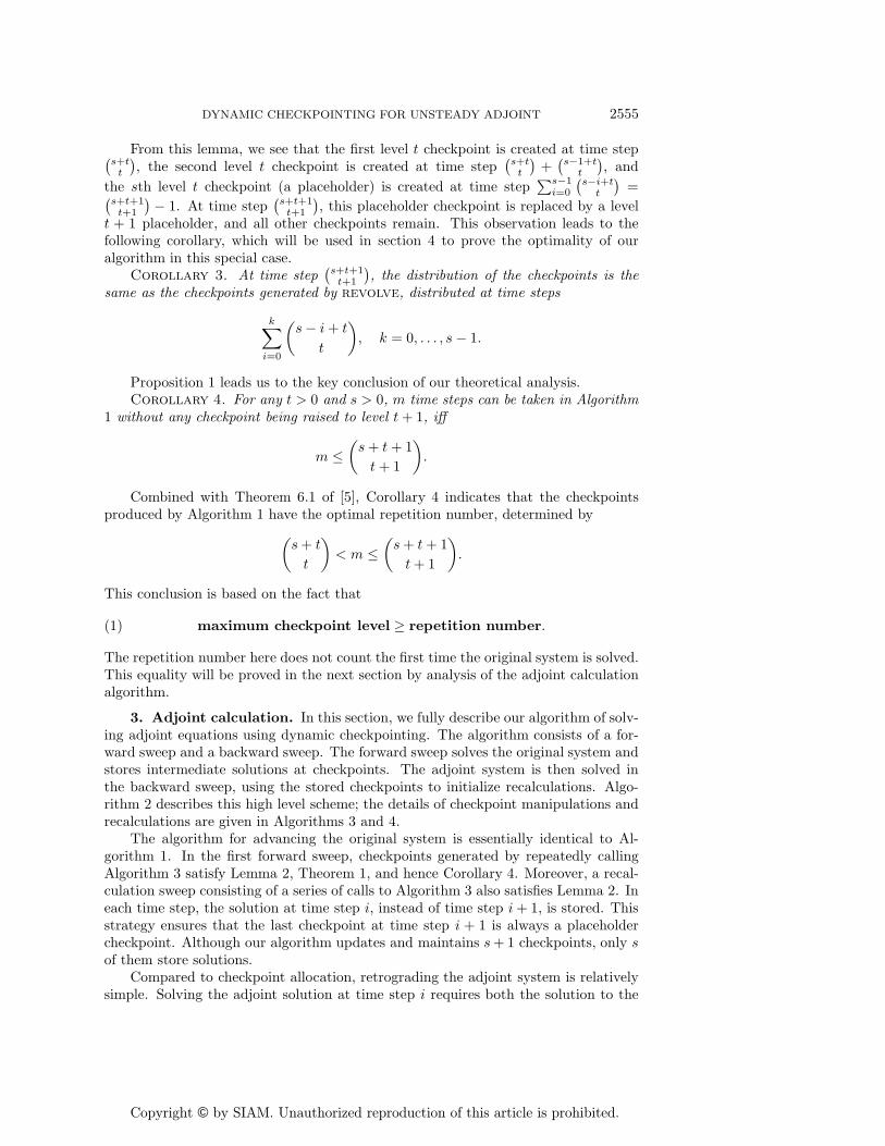
Fig. 1. Dynamic allocation of checkpoints for s = 3. The plot shows the checkpoints distributionduring 25 time steps of time integration. Each vertical cross-section on the plot represents a snapshotof the time integration history, from time step 0 to time step 25, indicated by the vertical axis.Different symbols represent different levels of checkpoints: Circles are level ∞ checkpoint at timestep 0. Thin dots, “+”, “×”, and star symbols correspond to level 0, 1, 2, and 3 checkpoints,respectively. The thick dots connected by a line indicate the time step index of the current solution,which is also the position of the placeholder checkpoint.

checkpoints, none of which are dispensable. The algorithm enters the “else” clausewith l = 0. In this clause, the checkpoint at time step s is removed, and time step s+1is saved as a level 1 checkpoint, making all checkpoints except for the first and last onesdispensable. As the time integration continues, these s − 1 dispensable checkpointsare then recycled, while time steps s + 2 to 2s take their place as level 0 checkpoints.A third checkpoint of level 1 is created for time step 2s+1, while the remaining s− 2level 0 checkpoints become dispensable. Each time a level 1 checkpoint is made, oneless level 0 checkpoint is dispensable, resulting in one less space between the currentand the next level 1 checkpoints. The s+1st level 1 checkpoint is created for time step(s+1)+ s+(s− 1)+ · · ·+2 =

(s+22

)− 1. At this point, all s+1 checkpoints are level

1, while the space between them is an arithmetic sequence. All checkpoints createdthus far are exactly the same as the online checkpointing algorithm [8], although theiralgorithm breaks down and produces an error at the very next time step.

Our algorithm continues by allocating a level 2 checkpoint for time step(s+22

). At

the same time, the level 1 checkpoint at time step(s+22

)−1 is deleted, and all other level

1 checkpoints become dispensable. A similar process of creating level 2 checkpointsensues. The third level 2 checkpoint is created for time step

(s+22

)+

(s+12

), after the

same evolution described in the previous paragraph with only s− 1 free checkpoints.The creation of level 2 checkpoints continues until the s + 1st level 2 checkpoint iscreated with time step index

(s+22

)+

(s+12

)+ · · ·+

(32

)=

(s+33

)−1. The creation of the

first level 3 checkpoint follows at time step(s+33

). Figure 1 illustrates an example of

this process where s = 3. Until now, we found that the time steps of the first level 0,1, 2, and 3 checkpoints are, respectively, 1, s + 1,

(s+22

), and

(s+33

). This interesting

pattern leads to our first proposition.Proposition 1. In Algorithm 1, the first checkpoint of level t is always created

for time step(s+t

t

).



To prove this proposition, we note that it is a special case of the following lemmawhen i = 0, making it only necessary to prove the lemma.

Lemma 2. In Algorithm 1, let i be the time step of a level t − 1 or highercheckpoint. The next checkpoint with level t or higher is at time step i +

(s−ni+t

t

)and is level t iff ni < s, where ni is the number of indispensable checkpoints allocatedbefore time step i.

Proof. We use induction here. When t = 0,(s−ni+t

t

)= 1. The next checkpoint

is allocated at time step i + 1, and its level is nonnegative; therefore, it is level 0 orhigher. If there is a dispensable checkpoint at time step i, the new checkpoint is level0; otherwise, it is level 1.

Assuming that the lemma holds true for any 0 ≤ t < t0, we now prove it fort = t0. Suppose ni = s. Then, no dispensable checkpoint exists. Therefore, at stepi +

(s−ni+t

t

)= i + 1, the (second) “else” clause is executed, creating a higher level

checkpoint at time step i + 1. The lemma holds in this case. Suppose ni < s, we usethe induction hypothesis. The next level t − 1 checkpoint is created at time step

i1 = i +(

t − ni + t − 1t − 1

),

incrementing the number of indispensable checkpoints

ni1 = ni + 1.

As a result, the following level t − 1 checkpoints are created at time steps

i2 = i1 +(

s − ni1 + t − 1t − 1

),

i3 = i2 +(

s − ni2 + t − 1t − 1

),

. . .

ik+1 = ik +(

s − nik+ t − 1

t − 1

),

. . . .

This creation of level t−1 checkpoints continues until nik= ni +k = s. At this point,

all existing checkpoints are level t − 1. Consequently, the “else” clause is executedwith l = t − 1 and creates the first level t checkpoint at time step

is−ni+1 = i +(

s − ni + t − 1t − 1

)+

(s − ni − 1 + t − 1

t − 1

)+ · · · +

(t − 1t − 1

).

Using Pascal’s rule

(m

k

)=

(m − 1

k

)+

(m − 1k − 1

)=

k∑i=0

(m − 1 − i

k − i

)

with m = s − ni + t and k = s − ni, this equation simplifies to

is−ni+1 = i +(

s − ni + t

t

),

which completes the induction.



From this lemma, we see that the first level t checkpoint is created at time step(s+t

t

), the second level t checkpoint is created at time step

(s+t

t

)+

(s−1+t

t

), and

the sth level t checkpoint (a placeholder) is created at time step∑s−1

i=0

(s−i+t

t

)=(

s+t+1t+1

)− 1. At time step

(s+t+1

t+1

), this placeholder checkpoint is replaced by a level

t + 1 placeholder, and all other checkpoints remain. This observation leads to thefollowing corollary, which will be used in section 4 to prove the optimality of ouralgorithm in this special case.

Corollary 3. At time step(s+t+1

t+1

), the distribution of the checkpoints is the

same as the checkpoints generated by revolve, distributed at time steps

k∑i=0

(s − i + t

t

), k = 0, . . . , s − 1.

Proposition 1 leads us to the key conclusion of our theoretical analysis.Corollary 4. For any t > 0 and s > 0, m time steps can be taken in Algorithm

1 without any checkpoint being raised to level t + 1, iff

m ≤(

s + t + 1t + 1

).

Combined with Theorem 6.1 of [5], Corollary 4 indicates that the checkpointsproduced by Algorithm 1 have the optimal repetition number, determined by

(s + t

t

)< m ≤

(s + t + 1

t + 1

).

This conclusion is based on the fact that

(1) maximum checkpoint level ≥ repetition number.

The repetition number here does not count the first time the original system is solved.This equality will be proved in the next section by analysis of the adjoint calculationalgorithm.

3. Adjoint calculation. In this section, we fully describe our algorithm of solv-ing adjoint equations using dynamic checkpointing. The algorithm consists of a for-ward sweep and a backward sweep. The forward sweep solves the original system andstores intermediate solutions at checkpoints. The adjoint system is then solved inthe backward sweep, using the stored checkpoints to initialize recalculations. Algo-rithm 2 describes this high level scheme; the details of checkpoint manipulations andrecalculations are given in Algorithms 3 and 4.

The algorithm for advancing the original system is essentially identical to Al-gorithm 1. In the first forward sweep, checkpoints generated by repeatedly callingAlgorithm 3 satisfy Lemma 2, Theorem 1, and hence Corollary 4. Moreover, a recal-culation sweep consisting of a series of calls to Algorithm 3 also satisfies Lemma 2. Ineach time step, the solution at time step i, instead of time step i + 1, is stored. Thisstrategy ensures that the last checkpoint at time step i + 1 is always a placeholdercheckpoint. Although our algorithm updates and maintains s + 1 checkpoints, only sof them store solutions.

Compared to checkpoint allocation, retrograding the adjoint system is relativelysimple. Solving the adjoint solution at time step i requires both the solution to the



Algorithm 2 High level scheme to solve the adjoint equation.Initialize the original system;i ⇐ 0;Save time step 0 as a placeholder checkpoint of level ∞;while the termination criteria of the original system is not met do

Solve the original system from time step i to i + 1 using Algorithm 3;i ⇐ i + 1;

end whileInitialize the adjoint system;while i >= 0 do

i ⇐ i − 1;Solve the adjoint system from time step i + 1 to i using Algorithm 4;

end while.

Algorithm 3 Solving the original system from time step i to i + 1.Require: s > 0 given; solution at time step i has been calculated.

if the number of checkpoints <= s thenSave time step i + 1 as a checkpoint of level 0;

else if at least one checkpoint is dispensable thenRemove the dispensable checkpoint with the largest time step index;Save time step i + 1 as a checkpoint of level 0;

elsel ⇐ the level of checkpoint at time step i;Remove the checkpoint at time step i;Save time step i + 1 as a checkpoint of level l + 1;

end ifif time step i is in the current set of checkpoints then

Store the solution at time step i to the checkpoint;end ifCalculate time step i + 1 of the original system.

Algorithm 4 Solving the adjoint system from time step i + 1 to i.Require: s > 0 given; adjoint solution at time step i + 1 has been calculated.

Remove the placeholder checkpoint at time step i + 1;if the last checkpoint is at time step i then

Retrieve the solution at time step i, making it a placeholder checkpoint;else

Retrieve the solution at the last checkpoint, making it a placeholder check-point;Initialize the original system with the retrieved solution;Solve the original system to time step i by calling Algorithm 3;

end ifCalculate time step i of the adjoint system.

adjoint system at time step i+1 and the solution to the original system at time step i.The latter can be directly retrieved if there is a checkpoint for time step i; otherwise,it must be recalculated from the last saved checkpoint. Note that this algorithm callsAlgorithm 3 to recalculate the solution of the original system at time step i from



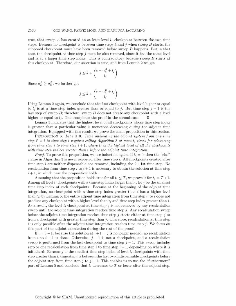
Fig. 2. Distribution of checkpoints during the process of Algorithm 2 for s ≥ 25. Each verticalcross-section on the plot represents a snapshot of the algorithm execution history, from the beginningof the forward sweep to the end of the adjoint sweep, indicated by the horizontal axis. Differentsymbols represent different levels of checkpoints: Circles are level ∞ checkpoint at time step 0. Thindots, “+”, “×”, and star symbols correspond to level 0, 1, 2, and 3 checkpoints, respectively. Theround, thick dots indicate the time step index of the current original solution, which is also theposition of the placeholder checkpoint; the lines connecting these round dots indicate where andwhen the original equation is solved. The thick dots with a small vertical bar indicate the time stepindex of the current adjoint solution, while the lines connecting them indicate where and when theadjoint equation is solved.

Fig. 3. Distribution of checkpoints during Algorithm 2 for s = 5. Refer to Figure 2 forexplanation of symbols.

the last saved checkpoint, during which more checkpoints are created between thelast saved checkpoint and time step i. These new checkpoints reduce the number ofrecalculations using memory space freed by removing checkpoints after time step i.

Figures 2–5 show examples of the entire process of Algorithm 2 with four differentvalues of s. As can be seen, the fewer the specified number of checkpoints s, the morerecalculations of the original equation are performed, and the longer it takes to solvethe adjoint equation. When s ≥ 25, there is enough memory to store every timestep, so no recalculation is done. The maximum finite checkpoint level is 0 in thiscase. When s = 6, the maximum finite checkpoint level becomes 1, and at most 1recalculation is done for each time step. When s decreases to 5 and 3, the maximumfinite checkpoint level increases to 2 and 3, respectively, and the maximum number





of recalculations also increases to 2 and 3, respectively. From these examples, we seethat the number of recalculations at each time step is bounded by the level of thecheckpoints after that time step. In the remaining part of this section, we focus onproving this fact, starting with Lemma 5.

Lemma 5. Denote ti as the highest level of all checkpoints whose time steps aregreater than i. For any i, ti does not increase for each adjoint step. Furthermore, ifi is between the time steps of the last two indispensable checkpoints before an adjointstep, ti decreases after this adjoint step.

Proof. Fix i, consider an adjoint step from time step j to j−1, where j > i. Notethat before this adjoint step, time step j is a placeholder checkpoint. Denote the levelof this checkpoint as lj . If time step j − 1 is stored in a checkpoint before this adjointstep, then checkpoint j is removed and all other checkpoints remain, making Lemma5 trivially true. If time step j − 1 is not stored before this adjoint step, the originalsystem is recalculated from the last checkpoint to time step j−1. We now prove thatthis recalculation sweep does not produce any checkpoints with level higher or equalto lj . As a result, ti does not increase; furthermore, if no other level ti checkpoint hasa time step greater than i, ti decreases.



Denote the time step of the last checkpoint as k and its level as lk. We use capitalletter B to denote the recalculation sweep in the current adjoint step. Note thatsweep B starts from time step k and ends at time step j − 1. On the other hand, thecheckpoint at time step j is created either during the first forward sweep or duringa recalculation sweep in a previous adjoint step. We use capital letter A to denote apart of this sweep from time step k to when the checkpoint at time step j is created.To compare the sweeps A and B, note the following two facts: First, the checkpointat time step k exists before sweep A. This is because sweep A created the checkpointat time step j, making all subsequent recalculations before sweep B start from eitherthis checkpoint or a checkpoint whose time step is greater than j. Consequently, thecheckpoint at time step k is not created after sweep A; it is created either by sweep Aor exists before sweep A. Secondly, because any sweep between A and B starts at timestep j or greater, it does not create any checkpoint with a time step index smallerthan k. On the other hand, any checkpoint removed during or after sweep A andbefore B is always the lowest level at that time, and thus, does not cause the increaseof the number of dispensable checkpoints. As a result, the number of dispensablecheckpoints with time step indices smaller than k is no less at the beginning of sweepA than at the beginning of sweep B. This is identical to stating

nAk ≥ nB

k ,

where nk is the number of indispensable checkpoints with time step indices less thank; the superscript identifies the sweep in which the indispensable checkpoints arecounted.

Now, we complete the proof by comparing sweeps A and B in the following twocases: If lk < lj, we assert that sweep A does not create any higher level checkpointthan lk at time steps between k and j. Suppose the contrary is true, that sweep Ahas created an at least level lk + 1 checkpoint between the two time steps. Becauseno checkpoint is between time steps k and j when sweep B starts, the supposedcheckpoint must have been removed before sweep B happens. But in that case, thecheckpoint at time step k must be also removed because its level is lower. Thiscannot happen because sweep B starts at this checkpoint. This contradiction provesour assertion. Because time step j is the first higher level checkpoint than lk createdby sweep A with larger time step index than k, its time step index, based on Lemma2, is

j = k +(

s − nAk + lk + 1lk + 1

).

Since nAk ≥ nB

k , we further get

j ≤ k +(

s − nBk + lk + 1lk + 1

).

Using Lemma 2 again, we conclude that the first checkpoint with level higher than lkis at a time step index greater than or equal to j. But time step j − 1 is the last stepof sweep B; therefore, sweep B does not create any checkpoint with a level higherthan lk. Since lk < lj , no level lj or higher checkpoint is created by sweep B. Thiscompletes the proof in the first case.

In the second case, lk ≥ lj, we assert that the checkpoint at time step j is thefirst one created by sweep A with level higher or equal to lj . Suppose the contrary is



true, that sweep A has created an at least level lj checkpoint between the two timesteps. Because no checkpoint is between time steps k and j when sweep B starts, thesupposed checkpoint must have been removed before sweep B happens. But in thatcase, the checkpoint at time step j must be also removed, since it has the same leveland is at a larger time step index. This is contradictory because sweep B starts atthis checkpoint. Therefore, our assertion is true, and from Lemma 2 we get

j ≤ k +(

s − nAk + ljlj

).

Since nAk ≥ nB

k , we further get

j ≤ k +(

s − nBk + ljlj

).

Using Lemma 2 again, we conclude that the first checkpoint with level higher or equalto lj is at a time step index greater than or equal to j. But time step j − 1 is thelast step of sweep B; therefore, sweep B does not create any checkpoint with a levelhigher or equal to lj . This completes the proof in the second case.

Lemma 5 indicates that the highest level of all checkpoints whose time step indexis greater than a particular value is monotone decreasing during the adjoint timeintegration. Equipped with this result, we prove the main proposition in this section.

Proposition 6. Let i ≥ 0. Time integrating the adjoint system from any timestep i′ > i to time step i requires calling Algorithm 3 at most ti times for advancingfrom time step i to time step i + 1, where ti is the highest level of all the checkpointswith time step indices greater than i before the adjoint time integration.

Proof. To prove this proposition, we use induction again. If ti = 0, then the “else”clause in Algorithm 3 is never executed after time step i. All checkpoints created aftertime step i are neither dispensable nor removed, including the i + 1st time step. Norecalculation from time step i to i + 1 is necessary to obtain the solution at time stepi + 1, in which case the proposition holds.

Assuming that the proposition holds true for all ti ≤ T , we prove it for ti = T +1.Among all level ti checkpoints with a time step index larger than i, let j be the smallesttime step index of such checkpoints. Because at the beginning of the adjoint timeintegration, no checkpoint with a time step index greater than i has a higher levelthan ti; by Lemma 5, the entire adjoint time integration from time step i′ to i does notproduce any checkpoint with a higher level than ti and time step index greater than i.As a result, the level ti checkpoint at time step j is not removed by any recalculationsweep until the adjoint time integration reaches time step j. Any recalculation sweepbefore the adjoint time integration reaches time step j starts either at time step j orfrom a checkpoint with greater time step than j. Therefore, recalculation at time stepi is only possible after the adjoint time integration reaches time step j. We focus onthis part of the adjoint calculation during the rest of the proof.

If i = j−1, because the solution at i+1 = j is no longer needed, no recalculationfrom i to i + 1 is done. Otherwise, j − 1 is not a checkpoint, and a recalculationsweep is performed from the last checkpoint to time step j − 1. This sweep includeszero or one recalculation from time step i to time step i + 1, depending on where it isinitialized. Because j is the smallest time step index of level ti checkpoints with timestep greater than i, time step i is between the last two indispensable checkpoints beforethe adjoint step from time step j to j − 1. This enables us to use the “furthermore”part of Lemma 5 and conclude that ti decreases to T or lower after this adjoint step.



Therefore, from our induction hypothesis, the number of recalculations at time stepi after this adjoint step is at most ti − 1. Combining this number with the possibleone recalculation during the adjoint step from j to j−1, the total recalculations fromtime step i to time step i + 1 during all the adjoint steps from time step i′ to i is atmost ti, completing our induction.

As a special case of the proposition, consider time step i′ to be the last time stepin solving the original system, and i = 0. Let t = t0 be the highest finite level of allcheckpoints when the first forward sweep is completed. According to the proposition,ti ≤ t for all i, resulting in the following corollary.

Corollary 7. In Algorithm 3, let t be the maximum finite checkpoint level afterthe original system is solved for the first time. Algorithm 4 is called at most t timesfor each time step during the backward sweep in solving the adjoint equation.

Corollary 7 effectively states (1). Combined with Corollary 4, it proves that ourdynamic checkpointing algorithm achieves a repetition number of t for

(s+t

t

)time

steps. This, as proven by [5], is the optimal repetition number for any checkpointingalgorithm.

4. Algorithm efficiency. The previous two sections presented our dynamiccheckpointing algorithm and its optimality in the repetition number. Here, we discussthe implication of this optimality on the performance of this algorithm, and demon-strate its efficiency using numerical experiments. We begin by providing a theoreticalupper bound on the total number of time step recalculations in our adjoint.

Proposition 8. The overall number of forward time step recalculations in theadjoint calculation nr is bounded by

(2) nr < t m −(

s + t

t − 1

),

where m is the number of time steps, t is the repetition number determined by(

s + t

t

)< m ≤

(s + t + 1

t + 1

),

and s is the number of allowed checkpoints.Proof. Since the repetition number is t, there is at least one checkpoint of level

t and no checkpoint of a higher level (Corollary 4). The first level t checkpoint iscreated at time step index

(s+t

t

), according to Proposition 1. Since no checkpoint of

a higher level is created, this first level t checkpoint cannot removed by Algorithm1. We split the adjoint calculation at the first level t checkpoint at time step index(s+t

t

). First, in calculating the adjoint steps of index from m to

(s+t

t

), every forward

step is recalculated at most t times by definition of the repetition number t. The totalnumber of forward time step recalculations in this part is less than or equal to

t

(m −

(s + t

t

)).

In fact it is always less than, since the very last time step is never recalculated. Second,in calculating the adjoint steps of index from

(s+t

t

)− 1 to 0, if no checkpoint exists in

this part, the total number of forward time step recalculations is

t

(s + t

t

)−

(s + t

t − 1

)



(equation (3) in [6]). The total number of recalculations in this part is less than thisnumber if there is one or more checkpoints between time step 0 and

(s+t

t

). Therefore,

the total number of forward time step recalculations in the entire adjoint calculation,which is the sum of the number of recalculations in the two parts, is less than

t m −(

s + t

t − 1

).

Having this upper bound, we compare the total number of recalculations of ouralgorithm with the optimal static checkpointing scheme. The minimum number oftotal forward time step calculations for an adjoint calculation of length m is

(t + 1)m −(

s + t + 1t

)

(equation (3) in [6]), including the m − 1 forward time step calculations before theadjoint calculation begins. Therefore, the minimum number of total recalculations is

(3) nr ≥ nr opt = t m −(

s + t + 1t

)+ 1.

Equations (2) and (3) bound the total number of forward time step recalculations ofour dynamic checkpointing scheme. They also bound the deviation from optimalityin terms of total recalculations:

nr − nr opt <

(s + t + 1

t

)−

(s + t

t − 1

)− 1 =

(s + t

t

)− 1.

This bound naturally leads to the following corollary.Corollary 9. Using our dynamic checkpointing scheme takes less total recalcu-

lations than running the simulation forward, determining the number of time steps,and then (knowing the time step count) using the proven optimal revolve algorithm.

Proof. Running the simulation forward to determine the number of time steps,then using revolve takes a total number of n′

r = m + nr opt recalculations. Sincem >

(s+t

t

), we have n′

r > nr opt +(s+t

t

)> nr.

In addition to this theoretical upper bound, the following proposition proves thatour scheme achieves an optimal number of recalculations in certain special cases.

Proposition 10. The total number of recalculations is optimal as in (3) when

m ≤(

s + 22

)or m =

(s + t

t

)for any t ≥ 2,

where m is the number of time steps.Proof. When m ≤ s, no recalculation is necessary, thus the result is trivially

true. When s < m ≤(s+22

), the repetition number t = 1. Therefore, each time step

is recalculated at most once. Furthermore, the s time steps stored as checkpointsare not recalculated, and the last time step is not recalculated. Therefore, the totalnumber of recalculations is no more than m − s − 1, which is the minimum numberof total recalculations when t = 1, according to (3). This proves the proposition form ≤

(s+22

).

We use induction to prove the proposition when m =(s+t+1

t+1

)for some t ≥ 1. We

have already proved the result when t = 1. Now assume that the proposition holds



Fig. 6. The horizontal axis is the number of time steps, and the vertical axis is the averagenumber of recalculations for each time step, defined as the total number of recalculations divided bythe number of time steps. Plus signs are the actual average number of recalculations of the dynamiccheckpointing scheme; the solid line and the dotted line are the lower and upper bound defined by(2) and (3). The upper left, upper right, lower left, and lower right plots correspond to 10, 25, 50,and 100 allowed checkpoints, respectively.

for t, i.e., the total number of recalculations is (t − 1)m −(

s+tt−1

)+ 1 when m =

(s+t

t

)for any s. Now when m =

(s+t+1

t+1

), Corollary 3 shows the checkpoints are distributed

at time step m0 = 0 and time steps mk =∑k−1

i=0

(s−i+t

t

), k = 1, . . . , s − 1. Marching

backwards from time step mk+1 to time step mk is the equivalent of marching(s−k+t

t

)time steps using s− k checkpoints, which takes

(s−k+t

t

)− 1 recalculations in the first

forward sweep, plus (t − 1)(s−k+t

t

)−

(s−k+t

t−1

)+ 1 recalculations (by the induction

hypothesis). Therefore, the total number of recalculations is

s−1∑k=0

t

(s − k + t

t

)−

(s − k + t

t − 1

)= t

(s + t + 1

t + 1

)−

(s + t + 1

t

)+ 1

by applying Pascal’s rule. Therefore, the total number of recalculations is optimal fort + 1, completing the induction.

With these theoretical results, we next study experimentally the actual numberof recalculations of our dynamic checkpointing algorithm. Figure 6 plots the actualnumber of forward time step recalculations, together with the upper and lower bounddefined by (2) and (3). The total number of recalculations is divided by the numberof time steps, and the resulting average number of recalculations for each time step isplotted. As can be seen, the actual number lies between the lower and upper bound,as predicted by the theory. Also, more points tend to be closer to the lower boundthan to the upper bound, and some points lie exactly on the lower bound. This meansthat our algorithm in most cases outperforms what Corollary 9 guarantees.

While the total number of recalculations of our dynamic checkpointing algorithmis not necessarily as small as static checkpointing schemes, the repetition numberis provably optimal in any situation. Table 1 shows the maximum number of time



Table 1

Maximum number of time steps for a fixed number of checkpoints and repetition number t.

t = 1 t = 2 t = 3 t = 4 t = 10

10 checkpoints 66 286 1001 3003 1.85 × 105

25 checkpoints 351 3276 23751 1.43 × 105 1.84 × 108

50 checkpoints 1326 23426 3.16 × 105 3.48 × 106 7.54 × 1010

100 checkpoints 5151 1.77 × 105 4.60 × 106 9.66 × 107 4.69 × 1013

steps our algorithm can proceed for a given number of checkpoints and number ofrecalculations (repetition number). The range of checkpoints are typical for most oftoday’s unsteady simulations in fluid mechanics, which range from 10 checkpointsin high fidelity multiphysics simulations where limited memory is a serious issue, to100 checkpoints in calculations where memory requirements are less stringent. Themaximum number of time steps is calculated by the formula

(s+t+1

t+1

), where s is

the number of checkpoints and t is the number of recalculations. As can be seen, thenumber of time steps grows very rapidly as either the checkpoints or the recalculationsincrease. With only 10 checkpoints, 5 to 7 recalculations should be sufficient for themajority of today’s unsteady flow simulations. With 100 checkpoints, only one or tworecalculations are needed to achieve the same number of time steps. With this manycheckpoints, our algorithm requires only three recalculations for 4.6× 106 time steps,much more than current calculations use.

To end this section, we use a numerical experiment to demonstrate that ouralgorithm is not only theoretically advantageous, but also highly efficient in practice.In this experiment, the original system is the inviscid Burgers’ equation

ut +12

(u2

)x

= 0, x ∈ [0, 1], t ∈ [0, 1];

u|t=0 = sin 2πx, u|x=0,1 = 0.

We discretize this partial differential equation with a first-order up-winding finite-volume scheme with 250 mesh volumes and use forward Euler time integration with afixed CFL number |umax|Δt

Δx . As the time integration proceeds, a shock wave forms atx = 0.5. The shock wave dissipates the solution, decreases the maximum wavespeed|u|max, and increases the size of each time step due to the fixed CFL number. As aresult, the number of time steps needed to proceed to t = 1 is not known a priori. Tovary the number of time steps, we chose five different CFL numbers ranging from 1.0to 0.002. The discrete adjoint equation of the original system is solved with initialand boundary conditions,

φ|t=1 = sin 2πx, φ|x=0,1 = 0.

Four different numbers of checkpoints, s = 10, 25, 50, and 100, were specified. Foreach s, we ran five calculations with different CFL numbers. We recorded the ratioof computation time between the backward sweep of solving adjoint system and theforward sweep of solving the original system. Because the computation time of theforward sweep is the cost of solving the original system alone, this ratio reflects theadditional cost of solving the adjoint equation. We compare the ratio with a theoreti-cal bound derived by assuming that solving an adjoint step requires the same amountof computation time as a forward step.2 Under this assumption, the computation

2This is not a valid assumption in general; therefore, the theoretical bounds are not true bounds.In our numerical experiment, an adjoint step sometimes can be cheaper than each forward step. Asa result, the computing time ratios may be out of the theoretical bounds, as can be seen in Figure 7.



Fig. 7. Comparison of theoretical bounds (dotted and solid lines) and experimental performance(plus markers) of our dynamic checkpointing adjoint solver. The top left, top right, bottom left, andbottom right plots correspond to s = 10, 25, 50, and 100, respectively.

time ratio of the backward sweep to the forward sweep is equal to the average numberof recalculations for each time step plus 1. Therefore, upper and lower bounds of thisratio can be calculated by (3) and (2).

Figure 7 plots this experimental time ratio with the theoretical bounds. The foursubplots correspond to the different number of checkpoints used. Each subplot showsthe resulting number of time steps and ratio of computation time for five different CFLnumbers. As can be seen, most of the experimental time ratios are within or close tothe theoretical bounds, indicating that our algorithm works in practice as efficientlyas theoretically proven. In this experiment, the computational cost of calculating alinear adjoint step may be smaller than solving a nonlinear Burgers’ step, which canexplain why some points lie below the theoretical lower bound.

5. Conclusion and discussion. We propose a checkpointing adjoint solver, in-cluding an algorithm for dynamically allocating checkpoints during the initial calcula-tion of the original system and subsequent recalculations. Its three main advantagesover previous algorithms are as follows: the number of time steps does not need to beknown beforehand; the number of recalculations is minimized; an arbitrary numberof time steps can be integrated. For an original system with no more than

(s+t

t

)time steps, each time step is calculated at most t times, as has been proven optimalin the previous literature on checkpointing schemes [5]. Despite the lengthy proofof this optimality, the algorithm itself is conceptually simple to implement and haswidespread applications in scientific and engineering simulations of complex systems,where adaptive time stepping is often desirable, if not necessary.

Although this paper is biased towards solving adjoint equations of time dependentdifferential equations, a more compelling application of our algorithm is in reversemode AD. Most scientific computation code contains “if” and “while” statements,making their length of execution uncertain a priori. Therefore, our dynamic check-



pointing algorithm can be more suitable than static optimal checkpointing algorithmsin these cases.

Although we proved that our dynamic checkpointing algorithm has the optimalrepetition number, it is not always optimal in terms of the total number of timestep recalculations. When the number of time steps is between

(s+22

)and

(s+33

), the

improved online checkpointing scheme [13] may outperform our algorithm. Therefore,our dynamic checkpointing algorithm can still be improved in terms of the totalnumber of recalculations by placing and replacing low level checkpoints in a moreplanned manner. Future research should be done in combining our algorithm withthe improved online checkpointing scheme. We think it is possible to use online

checkpointing until the number of time steps reaches(s+33

), then switch to our

algorithm to proceed.Our dynamic checkpointing algorithm aims only to optimize the repetition num-

ber and reduce the number of time step calculations, ignoring the computational costof writing and reading checkpoints. In many applications, such as solving incom-pressible Navier–Stokes equations where each time step involves solving a full Poissonequation, the cost of reading and writing checkpoints is negligible because calculatingeach time step takes much more computation time. In other cases, especially whenthe checkpoints are written in and read from a hard disk instead of being kept inRAM, the input/output time associated with checkpoint writing and reading cannotbe ignored. In such cases, our dynamic checkpointing algorithm may not be the bestchoice, since it requires significantly more checkpoint writing than revolve does.

An implicit assumption of our algorithm is the uniform cost of calculating eachtime step of the original system. Although this is true for the majority of simple partialdifferential equations, it is not true for some multiphysics simulations. Moreover,this assumption is false in some AD applications. While extension of this algorithmto account for the nonuniform cost of each time step should not be very difficult,maintaining a provable performance bound in the extension is subject to furtherinvestigation.

Another assumption on which we base our algorithm is that calculating the adjointsolution at time step i from time step i + 1 requires only the solution to the originalsystem at time step i. In practice, especially if advanced time integration methodsare used in solving the original equation, solving the discrete adjoint equation at timestep i may require more than one time step of the original system. Future researchplans includes investigating ways to adjust our algorithm for this case.

REFERENCES

[1] T. Bewley, P. Moin, and R. Temam, DNS-based predictive control of turbulence: An optimaltarget for feedback algorithms, J. Fluid Mech., 447 (2001), pp. 179–225.

[2] I. Charpentier, Checkpointing schemes for adjoint codes: Application to the meteorologicalmodel Meso-NH, SIAM J. Sci. Comput., 22 (2001), pp. 2135–2151.

[3] M. B. Giles and N. A. Pierce, Adjoint Error Correction for Integral Outputs, in ErrorEstimation and Adaptive Discretization Methods in Computational Fluid Dynamics, T. J.Barth and H. Deconinck, eds., Springer-Verlag, Heidelberg, 2002, pp. 47–96.

[4] M. B. Giles and E. Suli, Adjoint methods for PDEs: A posteriori error analysis and post-processing by duality, Acta Numer., 11 (2002), pp. 145–236.

[5] A. Griewank, Achieving logarithmic growth of temporal and spatial complexity in reverseautomatic differentiation, Optim. Methods Softw., 1 (1992), pp. 35–54.

[6] A. Griewank and A. Walther, Algorithm 799: Revolve: An implementation of checkpoint-ing for the reverse or adjoint mode of computational differentiation, ACM Trans. Math.Software, 26 (2000), pp. 19–45.



[7] A. Griewank and A. Walther, Evaluating Derivatives: Principles and Techniques of Algo-rithmic Differentiation, 2nd ed., SIAM, Philadelphia, PA, 2008.

[8] V. Heuveline and A. Walther, Online checkpointing for parallel adjoint computation inPDEs: Application to goal oriented adaptivity and flow control, in Proceedings of Euro-Par 2006 Parallel Processing, W. Nagel et al., ed., 2006, pp. 689–699.

[9] M. Hinze and J. Sternberg, A-Revolve: An adaptive memory- and run-time-reduced proce-dure for calculating adjoints; with an application to the instationary Navier-Stokes system,Optim. Methods Softw., 20 (2005), pp. 645–663.

[10] A. Jameson, Aerodynamic design via control theory, J. Sci. Comput., 3 (1988), pp. 233–260.[11] A. Kowarz and A. Walther, Optimal checkpointing for time-stepping procedures, in Pro-

ceedings of ICCS 2006, Lecture Notes in Comput. Sci. 3994, V. Alexandrov et al., ed.,Springer-Verlag, Berlin, 2006, pp. 541–549.

[12] N. Pierce and M. Giles, Adjoint recovery of superconvergent functionals from PDE approxi-mations, SIAM Rev., 42 (2000), pp. 247–264.

[13] P. Stumm and A. Walther, Towards the Economical Computation of Adjoints in PDEsusing Optimal Online Checkpointing, Technical report DFG-SPP 1253-15-04, DeutscheForschungsgemeinschaft Schwerpunktprogramm 1253, Bonn, Germany, 2008.

[14] Q. Wang, D. Gleich, A. Saberi, N. Etemadi, and P. Moin, A Monte Carlo method forsolving unsteady adjoint equations, J. Comp. Phys., 227 (2008), pp. 6184–6205.

OMPUT c - Massachusetts Institute of Technology

Documents

Transcript of OMPUT c - Massachusetts Institute of Technology