COMPETITIVENESS – A COMPARISON OF CHINA AND MEXICO

FELICITAS NOWAK-LEHMANN D. SEBASTIAN VOLLMER

IMMACULADA MARTÍNEZ-ZARZOSO

CESIFO WORKING PAPER NO. 2111 CATEGORY 10: EMPIRICAL AND THEORETICAL METHODS

OCTOBER 2007

PRESENTED AT CESIFO VENICE SUMMER INSTITUTE, WORKSHOP ON ‘THE MANY DIMENSIONS OF COMPETITIVENESS’, JULY 2007

An electronic version of the paper may be downloaded • from the SSRN website: www.SSRN.com • from the RePEc website: www.RePEc.org

• from the CESifo website: Twww.CESifo-group.org/wp T

brought to you by COREView metadata, citation and similar papers at core.ac.uk

provided by Research Papers in Economics

CESifo Working Paper No. 2111

COMPETITIVENESS – A COMPARISON OF CHINA AND MEXICO

Abstract Latin American countries have lost competitiveness in world markets in comparison to China over the last two decades. The main purpose of this study is to examine the causes of this development. To this end an augmented Ricardian model is estimated using panel data. The explanatory variables considered are productivity, unit labor costs, unit values, trade costs, price levels (in PPP), and real exchange rates in relative terms. Due to data restrictions, China’s relative exports (to the US, Argentina, Japan, Korea, UK, Germany, and Spain) will be compared to Mexico’s exports for a number of sectors over a period of eleven years. Panel and pooled estimation techniques (SUR-estimation, panel Feasible Generalized Least Squares (panel/pooled FGLS)) will be utilized to better control for country-specific effects (differences between American, Argentinian, Japanese, Korean, German, British, and Spanish markets), cross-section specific (sector-specific) effects, and correlation over time.

JEL Code: C23, F11, F14.

Keywords: Ricardian model of trade, panel data models, panel Feasible Generalized Least Squares, Seemingly Unrelated (SUR) estimation.

Felicitas Nowak-Lehmann D. Ibero-America Institute for Economic

Research University of Goettingen

Platz der Goettinger Sieben 3 Germany - 37073 Goettingen fnowak@uni-goettingen.de

Sebastian Vollmer Ibero-America Institute for Economic

Research & Center for Statistics University of Goettingen

Platz der Goettinger Sieben 3 Germany - 37073 Goettingen

Immaculada Martínez-Zarzoso Department of Economics and

Ibero-America Institute for Economic Research University of Goettingen

Platz der Goettinger Sieben 3 Germany - 37073 Goettingen

The authors would like to thank the participants of the CESifo Venice Summer Institute 2007 for their helpful comments. Sebastian Vollmer acknowledges financial support from the Georg Lichtenberg program “Applied Statistics & Empirical Methods”. Inmaculada Martínez-Zarzoso acknowledges financial support from Fundación Caja Castellón-Bancaja (P1-1B2005-33), Generalitat Valenciana (Grupos 03-151, INTECO and ACOMP 07/102) and the Spanish Ministry of Education (SEJ 2007-67548).

2

1. Introduction

Latin American countries have lost competitiveness in world markets in comparison to China

for the last two decades. The economic opening up of China, which was strategic and well

planned, included the attraction of foreign companies and their know-how through special

incentives such as tax exemptions, and through the creation of export-processing zones. Latin

American countries, in contrast, tried to pursue unilateral and regional trade liberalization

(creation of MERCOSUR, CAN, CACM). Their attempts to form Free Trade Agreements

(FTAs) with the European Union (EU) and the US have not yet yielded results. Overall, Latin

America’s strategic planning of exports aimed more towards signing bilateral trade

agreements (Mexico-EU, NAFTA, Chile-EU, Chile-US, etc.) with the objective to gain better

mutual market access and was less focused on foreign direct investment (FDI).

Due to China’s trade strategy, industrial development in the country has been rapid in contrast

to development in the farm sector. China’s top export sectors are automatic data-processing

machines, telecommunication equipment, baby carriages, toys, games, sporting goods,

footwear, and textiles. The best performing Chinese products in terms of export shares are

television cameras, video recording/ reproduction equipment, furniture, footwear, jerseys, and

pullovers (International Trade Center (ITC), based on COMTRADE statistics). China’s main

export markets are the US, Hong Kong, Japan, Republic of Korea, and Germany (UN

COMTRADE statistics database, 2006). In comparison with China, Latin American countries,

which are still strong in the agricultural and food-related sectors, lost influence in the

manufacturing, machinery, and transport equipment sectors between 1995 and 2000

(TradeCAN, 2002 Edition). Latin American countries export mainly to the US, Germany, the

Netherlands, France, Spain, and Portugal, according to UN COMTRADE statistics database,

2006.

3

The main purpose of this study is to examine the causes of this loss of Latin American trade

share and to measure the effects of relative productivity, changes in relative unit labor costs,

changes in relative unit values, and changes in the overall price level (in constant US dollar

terms) on relative export strength. If we find that the loss of Latin America’s competitiveness

is more the result of China’s exchange rate management, than any failure on the part of Latin

America, then Latin America would have less reason for concern. If, however, the loss of

competitiveness were more the result of China’s increase in productivity, then Latin America

should be concerned about its future standing in world markets.

There are few empirical studies attempting to disentangle the concepts of comparative and

competitive advantage when examining export success. This distinction, however, is crucial

for evaluating the development of market shares in certain sectors and certain markets, as well

as examining their determining factors. We build on a study by Golub and Hsieh (2000) who

empirically test the Ricardian model, explaining comparative advantage by differences in

productivity and labor costs. There is little empirical evidence based on the Ricardian model,

except for analyses by MacDougall (1951), Stern (1962), and Balassa (1963). Nonetheless,

the simplistic view of productivity differences as source of comparative advantage is

confirmed by international comparisons of productivity. The notion of competitive advantage,

in contrast, is the key concept of the newer trade theories and of strategic-trade policy and

continues to be a much-debated issue in developed and developing countries. After all, it is

costs (labor costs, trade costs--transport costs, tariff and non-tariff barriers, insurance costs))

and prices that matter in trade and, together, they are an important factor in determining the

success of a product even where product differentiation exists.

We try to extend the study of Golub and Hsieh (2000) by giving sectoral wages (unit labor

costs) and prices (unit export values) adequate importance and by including trade costs, price-

4

level indicators, and real exchange rates. We furthermore aim to identify sectors where

success is driven more by product quality than by product prices (in terms of export unit

values). An optimal model will therefore contain relative productivity, relative unit labor

costs, relative export unit values, differences in trade costs, a control for different price levels,

and different real exchange rates. Our study will build on a huge set of panel data and use

panel and pooled-estimation techniques (SUR-estimation, panel Feasible Generalized Least

Squares (panel/pooled FGLS)). In this panel data framework, we are able to control for

unobserved heterogeneity of various types (country-specific and sector-specific) and also for

time-driven effects.

In our analysis, we will limit ourselves to comparing China with a Latin American country

having a very strong manufacturing industry, namely Mexico, in selected single markets (US,

Japan, Korea, Germany, UK, Spain, and Argentina).1

2. Comparative and Competitive Advantage

We utilize an eclectic model that contains five components: comparative advantage, relative

trade costs, relative product prices (as measured by unit export values), relative overall price

levels at home and abroad, and relative real exchange rates. As to the first component,

comparative advantage, we build on a Ricardian model (the Scandinavian variant of the

Australian model (Salter, 1959; Swan, 1960, 1963)), in which labor is the only factor of

production and where home (nontraded) goods and traded goods are produced with constant

returns, (fixed coefficient production functions of the Leontieff-Walras type). Technology and

hence unit labor requirements differ across countries.

1 A comparison between China and Brazil was impaired by data problems (lack of comparable productivity

and labor compensation data) with respect to Brazil. Nonetheless, common to China and Mexico is the

influence of multinationals and foreign direct investment (FDI).

5

Following Dornbusch (1977, 1980), comparative advantage in the Ricardian model is

determined by unit labor requirements,

QLa /= (1)

where a is the number of units of labor required to produce a unit of value added ( Q ), and

L is labor employed when producing a product in the home country. The a , the inverse of

labor productivity, can be obtained from input-output tables.

The relative unit labor requirement A , our measure of comparative advantage, compares

technical efficiency at home and abroad2 (*) and is defined as

aaA /*≡ (2)

In a two-country, multi-good Ricardian model, comparative advantage can be determined by

ranking domestic and foreign labor productivity by sector (i =1,…, n).

nnii aaaaaaaa /.../...// **

2

*

21

*

1 >>>>> (3)

To make fair comparisons of competitiveness between the foreign and home markets, the

price of labor has to be viewed in a common currency since countries with low labor

productivity are well able to compete if their wages are sufficiently low and/or their exchange

rate is depreciated; analogously, countries with high labor productivity might be unable to

compete in international markets due to (excessively) high labor costs and/or an appreciated

exchange rate.

Relative unit labor costs ic , therefore, relate to cost/price competitiveness, our alternative first

component.

iiiii aweawc /**= (4)

2 In our empirical analysis, China stands for abroad and Mexico stands for home country.

6

where ic stands for relative labor unit costs and is a measure of competitive advantage. *

iw

and iw are labor costs (labor compensation) abroad and at home and e is the bilateral

nominal exchange rate between abroad and at home.

Sector i has a competitive advantage in the home country if

1>ic (5a)

or ii wa < ewa ii

** . (5b)

Under the assumption that the wage and price setting behavior at home and abroad is similar

(similar power of labor unions and similar profit margins, etc.), the ratio of relative unit

values )(UV3 and labor compensation

)//()*/*(

itw

itUVe

itw

itUV could serve as an indicator

of product quality, our second component. It could incorporate the aspects of differentiated

products having variable quality standards and diverse product characteristics.

Following Deardorff (2004), we extend the concept of comparative/competitive advantage

and control for trade costs itc , our third component, that arise when serving a certain market

m ( itcm ) . Taking into account trade costs, the home country will export a good to market m

if unit export values (including trade costs) are lower/less than abroad. To control for

differences in trade costs,4 we utilize the variable iii tcmetcmTCM −= )( * as an indicator for a

trade cost advantage/disadvantage. In the empirical analysis, we will use iTCM as a separate

variable and do not include it into the term ii UVUV /* .

3 sUV ' are normally in US dollars. If not, they must be converted to a common currency.

4 Trade costs can comprise tariffs, transport costs, insurance costs, and the like.

7

As to our fourth component, differing price levels at home (P) and abroad (P*), we will take a

look at the Purchasing Power Parity (PPP) theory. According to the PPP theory, prices (in a

common currency) for traded goods at home and abroad should be the same in the absence of

tariffs, transport costs, and the absence of spatial arbitrage, over the long run. In the short-to-

medium time period, however, a relatively lower price (or cost) level is expected to promote

trade.

We also accept that the market exchange rate e differs from the PPP exchange rate )( PPPe in

the short-to-medium term and that the short-to-medium term real exchange rate )(RER will

also differ from PPPRER . Thus the real exchange rate, our fifth component, can reflect the

impact of exchange-rate management over the short and medium term.

3. Empirical Implementation

3.1 Data and Variables

The main data source employed is World Bank’s database (http://www.worldbank.org/trade)

for sectoral exports in value and volume (1987-2004), export unit values (1987-2004), and

value added per employee (1980-1997).5 Sectoral data are organized according to the ISIC

classification which unites trade and production data. Macro data were taken from the World

Development Indicators of 2006. We used household final consumption expenditures per

capita (in constant 2000 US dollars) as a proxy for labor costs (1980-2004) and computed

bilateral real exchange rates (1980-2004) from WDI, 2006. The relative Chinese to Mexican

export values and unit values for the different destination markets are displayed in Figure 1 in

the example of the textiles sector.

5 Labor cost per employee (1980-1986) and unit labor costs (1980-1986) had too many missing values to

include them in the pooled analysis.

8

Figure 1 Development of relative export values (LXV) and relative unit values (LUV) for

textiles to all destination markets, in logs

0.0

0.5

1.0

1.5

2.0

2.5

87 88 89 90 91 92 93 94 95 96 97

Argentina

2.8

3.2

3.6

4.0

4.4

4.8

87 88 89 90 91 92 93 94 95 96 97

Germany

0.8

1.2

1.6

2.0

2.4

2.8

3.2

3.6

87 88 89 90 91 92 93 94 95 96 97

Spain

1.8

2.0

2.2

2.4

2.6

2.8

87 88 89 90 91 92 93 94 95 96 97

UK

5.0

5.5

6.0

6.5

7.0

7.5

8.0

87 88 89 90 91 92 93 94 95 96 97

Japan

-1

0

1

2

3

4

5

6

7

8

87 88 89 90 91 92 93 94 95 96 97

Korea

-0.8

-0.4

0.0

0.4

0.8

1.2

1.6

87 88 89 90 91 92 93 94 95 96 97

USA

LXV for Textiles

-1.4

-1.2

-1.0

-0.8

-0.6

-0.4

-0.2

0.0

0.2

87 88 89 90 91 92 93 94 95 96 97

Argentina

0.2

0.4

0.6

0.8

1.0

1.2

1.4

87 88 89 90 91 92 93 94 95 96 97

Germany

-.7

-.6

-.5

-.4

-.3

-.2

-.1

.0

.1

.2

87 88 89 90 91 92 93 94 95 96 97

Spain

-1.0

-0.5

0.0

0.5

1.0

87 88 89 90 91 92 93 94 95 96 97

UK

-1.2

-0.8

-0.4

0.0

0.4

0.8

1.2

1.6

87 88 89 90 91 92 93 94 95 96 97

Japan

-.3

-.2

-.1

.0

.1

.2

.3

.4

.5

.6

87 88 89 90 91 92 93 94 95 96 97

Korea

-1.2

-0.8

-0.4

0.0

0.4

0.8

1.2

87 88 89 90 91 92 93 94 95 96 97

USA

LUV for Textiles

Distances were taken from http://www.maritimeChain.com/ and freight costs (based on

Hufbauer, 1991, and Busse, 2003) were available from 1980 to 2004. A trade-cost variable is

computed by multiplying the freight-cost index with the difference in actual nautical miles

9

(the actual sea route that captains take) between the Chinese port and the Mexican port that is

used by ships going to a certain market, e.g., the US.

We have the unfortunate situation of having data for relative productivity (LVA) from 1980 to

1997 and having relative export values (LXV) and relative unit values (LUV) from 1987 to

2004. The relevant sample period thus shrinks to 1987 to 1997. This is not long enough to use

some specific estimation techniques examining all sectors (e.g.,system-of-equation

techniques (such as SUR) cannot be utilized in some sectors due to a lack of observations).

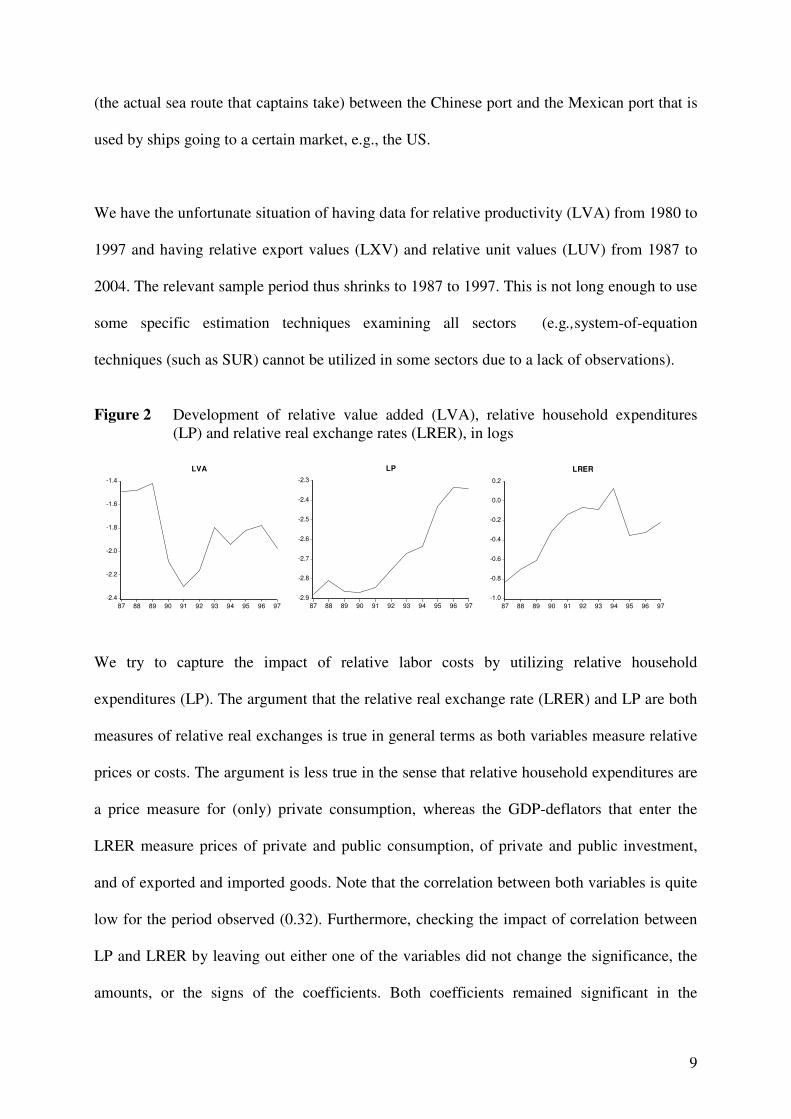
Figure 2 Development of relative value added (LVA), relative household expenditures

(LP) and relative real exchange rates (LRER), in logs

-2.4

-2.2

-2.0

-1.8

-1.6

-1.4

87 88 89 90 91 92 93 94 95 96 97

LVA

-2.9

-2.8

-2.7

-2.6

-2.5

-2.4

-2.3

87 88 89 90 91 92 93 94 95 96 97

LP

-1.0

-0.8

-0.6

-0.4

-0.2

0.0

0.2

87 88 89 90 91 92 93 94 95 96 97

LRER

We try to capture the impact of relative labor costs by utilizing relative household

expenditures (LP). The argument that the relative real exchange rate (LRER) and LP are both

measures of relative real exchanges is true in general terms as both variables measure relative

prices or costs. The argument is less true in the sense that relative household expenditures are

a price measure for (only) private consumption, whereas the GDP-deflators that enter the

LRER measure prices of private and public consumption, of private and public investment,

and of exported and imported goods. Note that the correlation between both variables is quite

low for the period observed (0.32). Furthermore, checking the impact of correlation between

LP and LRER by leaving out either one of the variables did not change the significance, the

amounts, or the signs of the coefficients. Both coefficients remained significant in the

10

regression when both variables were in the regression, and the size stayed practically

unaltered. The development of these dependent variables is displayed in Figure 2.

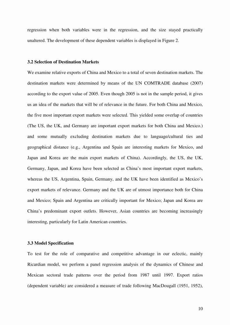
3.2 Selection of Destination Markets

We examine relative exports of China and Mexico to a total of seven destination markets. The

destination markets were determined by means of the UN COMTRADE database (2007)

according to the export value of 2005. Even though 2005 is not in the sample period, it gives

us an idea of the markets that will be of relevance in the future. For both China and Mexico,

the five most important export markets were selected. This yielded some overlap of countries

(The US, the UK, and Germany are important export markets for both China and Mexico.)

and some mutually excluding destination markets due to language/cultural ties and

geographical distance (e.g., Argentina and Spain are interesting markets for Mexico, and

Japan and Korea are the main export markets of China). Accordingly, the US, the UK,

Germany, Japan, and Korea have been selected as China’s most important export markets,

whereas the US, Argentina, Spain, Germany, and the UK have been identified as Mexico’s

export markets of relevance. Germany and the UK are of utmost importance both for China

and Mexico; Spain and Argentina are critically important for Mexico; Japan and Korea are

China’s predominant export outlets. However, Asian countries are becoming increasingly

interesting, particularly for Latin American countries.

3.3 Model Specification

To test for the role of comparative and competitive advantage in our eclectic, mainly

Ricardian model, we perform a panel regression analysis of the dynamics of Chinese and

Mexican sectoral trade patterns over the period from 1987 until 1997. Export ratios

(dependent variable) are considered a measure of trade following MacDougall (1951, 1952),

11

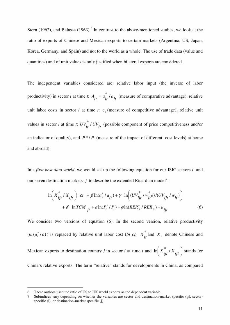
Stern (1962), and Balassa (1963).6 In contrast to the above-mentioned studies, we look at the

ratio of exports of Chinese and Mexican exports to certain markets (Argentina, US, Japan,

Korea, Germany, and Spain) and not to the world as a whole. The use of trade data (value and

quantities) and of unit values is only justified when bilateral exports are considered.

The independent variables considered are: relative labor input (the inverse of labor

productivity) in sector i at time t: it

ait

ait

A /*= (measure of comparative advantage), relative

unit labor costs in sector i at time t: itc (measure of competitive advantage), relative unit

values in sector i at time t: it

UVit

UV /* (possible component of price competitiveness and/or

an indicator of quality), and PP /* (measure of the impact of different cost levels) at home

and abroad).

In a first best data world, we would set up the following equation for our ISIC sectors i and

our seven destination markets j to describe the extended Ricardian model7:

ijtX

ijtX /*ln =

++ )//()*/*(ln)/ln( *

itw

ijtUVe

itw

ijtUV

itaait γβα

ijt

uRERRERPPjt

TCM jtjttt ++++ )/ln()/ln(ln ** φεδ (6)

We consider two versions of equation (6). In the second version, relative productivity

(ln )/( *aai ) is replaced by relative unit labor cost (ln ci).

*it

X and itX denote Chinese and

Mexican exports to destination country j in sector i at time t and

ijtX

ijtX /*ln stands for

China’s relative exports. The term “relative” stands for developments in China, as compared

6 These authors used the ratio of US to UK world exports as the dependent variable.

7 Subindices vary depending on whether the variables are sector and destination-market specific (ij), sector-

specific (i), or destination-market specific (j).

12

to Mexico. We build a system of seven equations describing China’s and Mexico’s

competitiveness in the markets of Argentina, Germany, Spain, UK, Japan, Korea, and the US.

We expect a relative increase in Chinese technical inefficiency and a relative increase in

Chinese unit labor costs to impact negatively on China’s competitiveness. Therefore, we

expect β to be negative. A bigger relative difference between unit export values and labor

compensation could have either a negative sign (when consumers predominantly consider

prices) or a positive sign (if consumers emphasize product quality). Furthermore, we think

that an increase in China’s relative trade costs will reduce China’s relative exports and that a

relative increase in China’s cost and price level (proxied by household expenditures) will

negatively impact China’s competitiveness. Accordingly, we expect a negative δ and a

negative ε . A relative increase in China’s real exchange rate (a depreciation of *RER in

relation to RER ) is supposed to promote China’s relative exports. We therefore expect a

positive φ .

Unfortunately, data restrictions concerning China, in particular, are severe (labor costs and,

consequently, unit labor costs, are available only for the short time span of 1980 through

1986, whereas export volumes and values are only available from 1987 onwards. In a second

best data world, we are therefore forced to reformulate our extended Ricardian model in the

following way:

=ijtlxv βα +j itlva ijtjttjtijt ulrerlpTCMluv +⋅+⋅+⋅++ φεδγ (7)

where =ijtlxv

ijtX

ijtX /*ln = relative exports to market j in millions of US dollars (USD)

(in logs); )/ln( *

ititit VAVAlva = = relative labor productivity (in logs) (the inverse of relative

input coefficients). We expect a positive sign; )/ln( *

ijtijtijt UVUVluv = = relative unit export

values in logs.

13

The expected sign is negative if price competitiveness prevails and positive if product quality

is emphasized; jtTCM = difference in transport costs (calculated as the difference between

China’s and Mexico’s difference in distances times a freight cost index; this variable’s impact

can be positive or negative depending on the destination market8, )/ln( *

ttt PPlp = = relative

household consumption expenditure per capita (constant 2000 USD) in logs, also an indicator

of relative costs. The expected sign is negative; )/ln( *

jtjtjt RERRERlrer = in logs with the

base year 2000. For the ratio of China’s and Mexico’s bilateral real exchange rate with respect

to the destination market j; the expected sign is positive. The World Bank’s database contains

twenty-eight ISIC sectors. A few sectors have been withdrawn from the analysis due to severe

data problems.

3.4 Estimation Procedure

The estimation procedure can be described as follows: In the first step, a pooled regression is

run to get an overview of the relevant variables in each sector. This model-setup is estimated

by Feasible Generalized Least Squares (FGLS), thus controlling for autocorrelation and non-

stationarity of the series.

In the second step, a system of equations is built around the seven destination markets

(Argentina, US, Germany, Spain, UK, Japan, and Korea). We control for correlation of the

disturbances between the cross-sections (the above-mentioned seven countries) via Seemingly

Unrelated Regression (SUR). By means of this method, correlation between the seven

destination markets is considered. The system approach adds supplementary information to

the non-system approach which was initially tested. The seven regressions (over the twenty-

eight sectors for each destination market) yielded quite poor results.

8 No logs are taken. Unfortunately, sector-specific transport costs are not available. Availability of sector-

specific transport costs would enrich the model and probably improve the explanatory power of our model.

14

In the third step, the system of equations is estimated with cross-section specific (country-

specific) coefficients. However, it is only possible to use this method when sufficient data are

available (such as in the textile sector).

4. Empirical Results: The Determinants of Competitiveness at the Sectoral Level

We present estimated results starting with a sector of utmost importance, namely textiles,

where our data on export values and unit values were relatively more complete. Equation (9)

was estimated with cross-section specific intercepts (country-fixed effects) and

autocorrelation was controlled for with an AR(1) term. Adjusted R2 was 0.92 and the Durbin-

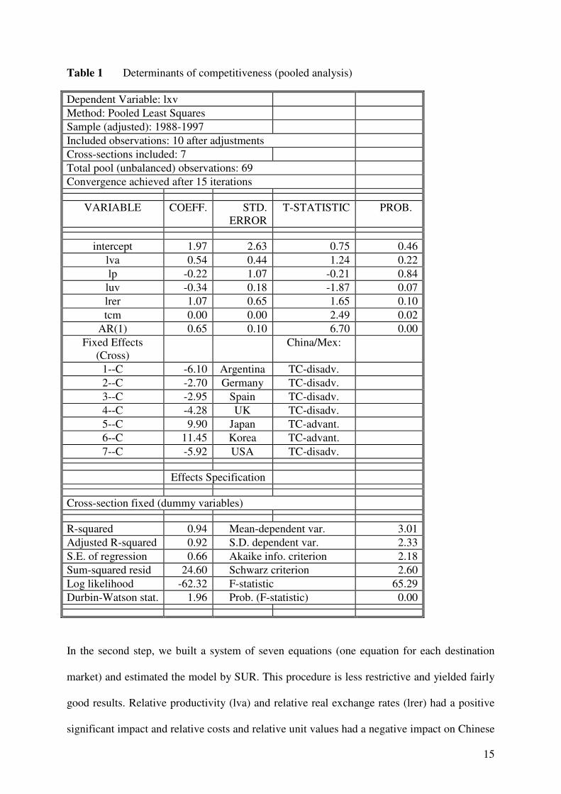
Watson statistic was 1.96 (see Table 1).

The signs of the coefficients are as expected, except for the variable TCM (transport cost

disadvantage). This coefficient was supposed to be negative but it turned out to be zero,

indicating that transport costs do not influence the Chinese-Mexican relationship in

competitiveness. 9

We observed that the transport cost effect was very well reflected in the

cross-section-specific intercepts. The intercepts were negative for the destination markets: the

US, Argentina, Germany, Spain, and UK, where China has a transport cost disadvantage, and

were positive for the destination markets Japan and Korea, where China has a transport cost

advantage. Relative productivity (lva) and our proxy for labor costs (lp) were insignificant but

show the correct sign. Relative unit values (luv) had a significant negative impact on relative

exports, implying that an increase in Chinese relative unit prices leads to a decrease in

Chinese relative exports. A depreciation of the relative real exchange rate (lrer) had a positive

impact on relative Chinese exports.

9 In fact, transport costs were zero or very close to zero for all twenty-eight ISIC sectors. Therefore,

transportation costs were removed from the regression equations. The “zero”-impact might be due to the fact

that we were forced to use to sector-unspecific transport costs due to unavailability of the data.

15

Table 1 Determinants of competitiveness (pooled analysis)

Dependent Variable: lxv

Method: Pooled Least Squares

Sample (adjusted): 1988-1997

Included observations: 10 after adjustments

Cross-sections included: 7

Total pool (unbalanced) observations: 69

Convergence achieved after 15 iterations

VARIABLE COEFF. STD.

ERROR

T-STATISTIC PROB.

intercept 1.97 2.63 0.75 0.46

lva 0.54 0.44 1.24 0.22

lp -0.22 1.07 -0.21 0.84

luv -0.34 0.18 -1.87 0.07

lrer 1.07 0.65 1.65 0.10

tcm 0.00 0.00 2.49 0.02

AR(1) 0.65 0.10 6.70 0.00

Fixed Effects

(Cross)

China/Mex:

1--C -6.10 Argentina TC-disadv.

2--C -2.70 Germany TC-disadv.

3--C -2.95 Spain TC-disadv.

4--C -4.28 UK TC-disadv.

5--C 9.90 Japan TC-advant.

6--C 11.45 Korea TC-advant.

7--C -5.92 USA TC-disadv.

Effects Specification

Cross-section fixed (dummy variables)

R-squared 0.94 Mean-dependent var. 3.01

Adjusted R-squared 0.92 S.D. dependent var. 2.33

S.E. of regression 0.66 Akaike info. criterion 2.18

Sum-squared resid 24.60 Schwarz criterion 2.60

Log likelihood -62.32 F-statistic 65.29

Durbin-Watson stat. 1.96 Prob. (F-statistic) 0.00

In the second step, we built a system of seven equations (one equation for each destination

market) and estimated the model by SUR. This procedure is less restrictive and yielded fairly

good results. Relative productivity (lva) and relative real exchange rates (lrer) had a positive

significant impact and relative costs and relative unit values had a negative impact on Chinese

16

relative exports, as expected. Table 2 shows the SUR results for all seven destination markets

together.

Table 2 Determinants of competitiveness in seven markets (dependent variable lxv)

VARIABLE COEFFICIENT T-STATISTIC P-VALUE

lva 0.52* 1.81 0.08

lp -1.20* -1.93 0.06

luv -0.14 -1.34 0.19

lrer 0.78* 1.81 0.07

Total system obs: 69 1 weight matrix R2 = 0.39

Sample: 1988-1997 21 total coef.

iterations

DW=1.54

Note: An AR(1) term was added. The coefficient was 0.78 and significant.

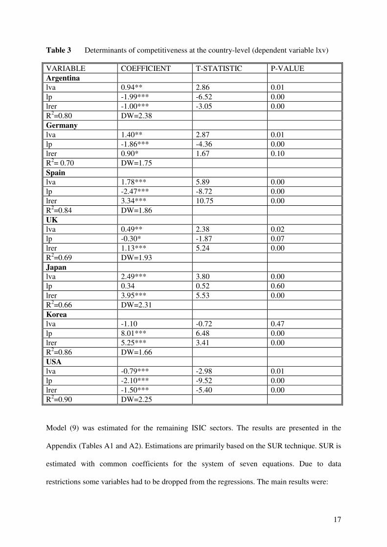
In the third step, a SUR was estimated with country-specific coefficients. luv was removed

from the variable list, since it was statistically insignificant. Table 3 shows the SUR results for

each of the seven countries.

We observe in Table 3 that almost all variables are significant (at conventional confidence

levels). Furthermore, the Durbin-Watson statistics are now closer to two and the explanatory

power of the regression equations has improved. The main message of Tables 1 to 3 is that the

impact of transport costs is captured by the intercept of the pooled regression (see Table 1,

Fixed Effects). China’s transport cost disadvantage is reflected in the negative intercept of

Argentina, Germany, Spain, UK, and the US, and China’s transport cost advantage is

reflected in the positive intercept of Japan and Korea. Low unit values (proxy for prices) of a

textile product enhance textile exports, α being twenty percent (Table 2). In summary, for

most countries, productivity, low costs, and a depreciated real exchange rate positively

influence competitiveness in the textile sector. Although, a seemingly unrelated regression

with country specific coefficients would be our model of choice, we have to admit that the

results have to be handled very carefully due to the data limitations discussed before.

17

Table 3 Determinants of competitiveness at the country-level (dependent variable lxv)

VARIABLE COEFFICIENT T-STATISTIC P-VALUE

Argentina

lva 0.94** 2.86 0.01

lp -1.99*** -6.52 0.00

lrer -1.00*** -3.05 0.00

R2=0.80 DW=2.38

Germany

lva 1.40** 2.87 0.01

lp -1.86*** -4.36 0.00

lrer 0.90* 1.67 0.10

R2= 0.70 DW=1.75

Spain

lva 1.78*** 5.89 0.00

lp -2.47*** -8.72 0.00

lrer 3.34*** 10.75 0.00

R2=0.84 DW=1.86

UK

lva 0.49** 2.38 0.02

lp -0.30* -1.87 0.07

lrer 1.13*** 5.24 0.00

R2=0.69 DW=1.93

Japan

lva 2.49*** 3.80 0.00

lp 0.34 0.52 0.60

lrer 3.95*** 5.53 0.00

R2=0.66 DW=2.31

Korea

lva -1.10 -0.72 0.47

lp 8.01*** 6.48 0.00

lrer 5.25*** 3.41 0.00

R2=0.86 DW=1.66

USA

lva -0.79*** -2.98 0.01

lp -2.10*** -9.52 0.00

lrer -1.50*** -5.40 0.00

R2=0.90 DW=2.25

Model (9) was estimated for the remaining ISIC sectors. The results are presented in the

Appendix (Tables A1 and A2). Estimations are primarily based on the SUR technique. SUR is

estimated with common coefficients for the system of seven equations. Due to data

restrictions some variables had to be dropped from the regressions. The main results were:

18

In furniture trade lower relative costs and a more depreciated real exchange rate influenced

Chinese exports positively. With respect to trade in iron and steel and non-ferrous metals,

lower unit values and a depreciated real exchange rate had a positive impact on China’s

exports. Product quality (as reflected by higher unit values) was rewarded by an increase in

Chinese fabricated metal exports as was a depreciated real exchange rate. Unit values did not

play a significant role in China’s exports of electric and non-electric machinery. A

depreciated real exchange helped to some extent. Concerning food exports, low unit values

determine export success. Consumers look for cheap nutrition. This may explain the success

of low price supermarkets. In the trade of wearing apparel, in contrast, only a depreciated

real exchange rate matters. Trade in industrial chemicals is positively determined by high

productivity, low unit prices and a favorable real exchange rate, whereas trade in beverages

profits from low costs in the production countries.

5. Conclusions

Even though the results reflect the heterogeneity of the ISIC sectors under examination, they

do show that comparative advantage of the Ricardo type is relevant in some sectors (textiles

and industrial chemicals). It also becomes evident that low cost countries do have a

competitive advantage, at least in some export sectors (textiles, furniture, beverages). Low

unit prices are important for export success in non-ferrous metals and food but they are

unimportant in the majority of the other sectors under investigation. Almost all sectors do

benefit from competitive real exchange rates what makes a prudent exchange rate

management so attractive. In this study the impact of transports costs seems to be captured in

the cross-section fixed effects (in the country fixed effects). Using a common intercept

transport costs are significant and carry the correct sign10

.

10 In preliminary estimations with a common intercept for all seven countries the transport cost coefficient was

significant, but the fixed effect model is better able to control for all sorts of country-specific characteristics.

19

Further research would be desirable on the cost side (labor costs, unit labor costs) of the

analysis. We would have especially appreciated to have longer time spans thus making our

estimation results more reliable. However, at the present time there are many data limitations

that prevent utilization of the more sophisticated model (eq. (8)).

20

References

Balassa, B. (1963) “An empirical demonstration of classical comparative cost theory”, The

Review of Economics and Statistics 4, 231-238.

Bureau of Labor Statistics (2007) “International Comparisons of Hourly Compensation Costs

for Production Workers in Manufacturing, 2005, http://www.bls.gov/fls (March 27,

2007), United States Labor Department, Washington, D.C.

Busse, M. (2003) “Tariffs, Transport Costs and the WTO Doha Round: The Case of

Developing Countries”, The Estey Centre Journal of International Law and Trade:

4:15-31.

Ceglowski, J. and S. Golub (2007) “Just How Low are China’s Labour Costs?”, The World

Economy : 597-617.

Choudri, E.U. and Schembri, L.L. (2002) “Productivity performance and international

competitiveness: Am old test reconsidered”, Canadian Journal of Economics 35(2);

341-362.

Cunat, A. (2005) “Can comparative advantage explain the growth of US trade?”, Centre for

Economic Policy Research, London.

Deardorff, A.V. (2004) “Local comparative advantage: Trade costs and the pattern of trade,

Research Seminar in International Economics, Discussion Paper No. 500, University

of Michigan.

Dornbusch, R., S. Fischer and P.A. Samuelson (1977), “Comparative Advantage, Trade, and

Payments in a Ricardian Model with a Continuum of Goods”, American Economic

Review Vol. 67: 823-839.

Dornbusch, R. (1980) Open Economy Macroeconomics, Basic Books, Inc. Publishers: New

York.

Drysdale, P. (2001) “Evidence of shifts in the determinants of Japanese manufacturing trade,

1970-1995. Australia-Japan Research Centre, Canberra.

21

Dullien; S. (2006) “China’s Changing Competitive Position: Lessons from a Unit-Labor-

Cost-Based REER, http://www.dullien.net/pdfs/ulcchina.pdf ( March 28, 2007)

Golub, S.S. (1994) “Comparative Advantage, Exchange Rates, and Sectoral Trade Balances

of Major Industrial Countries”, IMF Staff Papers Vol. 41, No. 2: 286-313.

Golub, S.S. and Hsieh, C.-T. (2000) “Classical Ricardian theory of comparative advantage

revisited” Review of International Economics 8(2), 221-234.

Hufbauer, G. (1991) “World Economic Integration: The Long View” International Economic

Insights 2(3):26-27.

Lett, E. and J. Banister (2006) “Labor costs of manufacturing employees in China: an update

to 2003-2004. Monthly Labor Review, November 2006, http://www.bls.gov/fls

(March 27, 2007), United States Labor Department, Washington, D.C.

Lewis, D. (2001) “International trade and comparative advantage in the Caribbean: an

empirical analysis, Journal of Eastern Caribbean Studies 26(1): 45-65.

Lücke, M. and J. Rothert (2006) “Central Asia’s comparative advantage in international

trade”, Kiel Economic Policy Papers. March 2006.

MacDougall, J. (1951) “British and American exports: A study suggested by the theory of

comparative costs, Part I”, The Economic Journal 61, 697-724.

MacDougall, J. (1952) “British and American exports: A study suggested by the theory of

comparative costs, Part II”, The Economic Journal 62 487-521.

Stern, D. (1962) “ British and American productivity and comparative costs in international

trade” Oxford Economic Papers 14, 275-296.

22

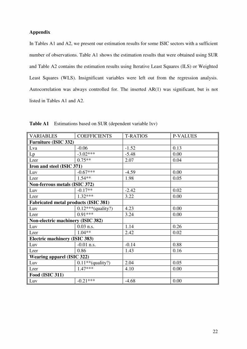
Appendix

In Tables A1 and A2, we present our estimation results for some ISIC sectors with a sufficient

number of observations. Table A1 shows the estimation results that were obtained using SUR

and Table A2 contains the estimation results using Iterative Least Squares (ILS) or Weighted

Least Squares (WLS). Insignificant variables were left out from the regression analysis.

Autocorrelation was always controlled for. The inserted AR(1) was significant, but is not

listed in Tables A1 and A2.

Table A1 Estimations based on SUR (dependent variable lxv)

VARIABLES COEFFICIENTS T-RATIOS P-VALUES

Furniture (ISIC 332)

Lva -0.06 -1.52 0.13

Lp -3.02*** -5.48 0.00

Lrer 0.75** 2.07 0.04

Iron and steel (ISIC 371)

Luv -0.67*** -4.59 0.00

Lrer 1.54** 1.98 0.05

Non-ferrous metals (ISIC 372)

Luv -0.17** -2.42 0.02

Lrer 1.32*** 3.22 0.00

Fabricated metal products (ISIC 381)

Luv 0.12***(quality?) 4.23 0.00

Lrer 0.91*** 3.24 0.00

Non-electric machinery (ISIC 382)

Luv 0.03 n.s. 1.14 0.26

Lrer 1.04** 2.42 0.02

Electric machinery (ISIC 383)

Luv -0.01 n.s. -0.14 0.88

Lrer 0.86 1.43 0.16

Wearing apparel (ISIC 322)

Luv 0.11**(quality?) 2.04 0.05

Lrer 1.47*** 4.10 0.00

Food (ISIC 311)

Luv -0.21*** -4.68 0.00

23

Table A2 Estimation results based on ILS or WLS (dependent variable lxv)

VARIABLES COEFFICIENTS T-RATIOS P-VALUES

Industrial chemicals (ISIC 351) WLS

lva 1.51*** 3.66 0.00

luv -0.18** -2.55 0.02

lrer 2.68*** 3.36 0.00

Beverages (ISIC 313) ILS

lva 0.47 0.56 0.58

lp -1.30 -1.40 0.17

CESifo Working Paper Series for full list see Twww.cesifo-group.org/wp T (address: Poschingerstr. 5, 81679 Munich, Germany, office@cesifo.de)

___________________________________________________________________________ 2048 Daniel Becker and Michael Rauscher, Fiscal Competition in Space and Time: An

Endogenous-Growth Approach, July 2007 2049 Yannis M. Ioannides, Henry G. Overman, Esteban Rossi-Hansberg and Kurt

Schmidheiny, The Effect of Information and Communication Technologies on Urban Structure, July 2007

2050 Hans-Werner Sinn, Please Bring me the New York Times – On the European Roots of

Richard Abel Musgrave, July 2007 2051 Gunther Schnabl and Christian Danne, A Role Model for China? Exchange Rate

Flexibility and Monetary Policy in Japan, July 2007 2052 Joseph Plasmans, Jorge Fornero and Tomasz Michalak, A Microfounded Sectoral

Model for Open Economies, July 2007 2053 Vesa Kanniainen and Panu Poutvaara, Imperfect Transmission of Tacit Knowledge and

other Barriers to Entrepreneurship, July 2007 2054 Marko Koethenbuerger, Federal Tax-Transfer Policy and Intergovernmental Pre-

Commitment, July 2007 2055 Hendrik Jürges and Kerstin Schneider, What Can Go Wrong Will Go Wrong: Birthday

Effects and Early Tracking in the German School System, July 2007 2056 Bahram Pesaran and M. Hashem Pesaran, Modelling Volatilities and Conditional

Correlations in Futures Markets with a Multivariate t Distribution, July 2007 2057 Walter H. Fisher and Christian Keuschnigg, Pension Reform and Labor Market

Incentives, July 2007 2058 Martin Altemeyer-Bartscher, Dirk T. G. Rübbelke and Eytan Sheshinski, Policies to

Internalize Reciprocal International Spillovers, July 2007 2059 Kurt R. Brekke, Astrid L. Grasdal and Tor Helge Holmås, Regulation and Pricing of

Pharmaceuticals: Reference Pricing or Price Cap Regulation?, July 2007 2060 Tigran Poghosyan and Jakob de Haan, Interest Rate Linkages in EMU Countries: A

Rolling Threshold Vector Error-Correction Approach, July 2007 2061 Robert Dur and Klaas Staal, Local Public Good Provision, Municipal Consolidation,

and National Transfers, July 2007 2062 Helge Berger and Anika Holler, What Determines Fiscal Policy? Evidence from

German States, July 2007

2063 Ernesto Reuben and Arno Riedl, Public Goods Provision and Sanctioning in Privileged

Groups, July 2007 2064 Jan Hanousek, Dana Hajkova and Randall K. Filer, A Rise by Any Other Name?

Sensitivity of Growth Regressions to Data Source, July 2007 2065 Yin-Wong Cheung and Xing Wang Qian, Hoarding of International Reserves: Mrs

Machlup’s Wardrobe and the Joneses, July 2007 2066 Sheilagh Ogilvie, ‘Whatever Is, Is Right’?, Economic Institutions in Pre-Industrial

Europe (Tawney Lecture 2006), August 2007 2067 Floriana Cerniglia and Laura Pagani, The European Union and the Member States:

Which Level of Government Should Do what? An Empirical Analysis of Europeans’ Preferences, August 2007

2068 Alessandro Balestrino and Cinzia Ciardi, Social Norms, Cognitive Dissonance and the

Timing of Marriage, August 2007 2069 Massimo Bordignon, Exit and Voice. Yardstick versus Fiscal Competition across

Governments, August 2007 2070 Emily Blanchard and Gerald Willmann, Political Stasis or Protectionist Rut? Policy

Mechanisms for Trade Reform in a Democracy, August 2007 2071 Maarten Bosker and Harry Garretsen, Trade Costs, Market Access and Economic

Geography: Why the Empirical Specification of Trade Costs Matters, August 2007 2072 Marco Runkel and Guttorm Schjelderup, The Choice of Apportionment Factors under

Formula Apportionment, August 2007 2073 Jay Pil Choi, Tying in Two-Sided Markets with Multi-Homing, August 2007 2074 Marcella Nicolini, Institutions and Offshoring Decision, August 2007 2075 Rainer Niemann, The Impact of Tax Uncertainty on Irreversible Investment, August

2007 2076 Nikitas Konstantinidis, Gradualism and Uncertainty in International Union Formation,

August 2007 2077 Maria Bas and Ivan Ledezma, Market Access and the Evolution of within Plant

Productivity in Chile, August 2007 2078 Friedrich Breyer and Stefan Hupfeld, On the Fairness of Early Retirement Provisions,

August 2007 2079 Scott Alan Carson, Black and White Labor Market Outcomes in the 19th Century

American South, August 2007

2080 Christian Bauer, Paul De Grauwe and Stefan Reitz, Exchange Rates Dynamics in a

Target Zone – A Heterogeneous Expectations Approach, August 2007 2081 Ana Rute Cardoso, Miguel Portela, Carla Sá and Fernando Alexandre, Demand for

Higher Education Programs: The Impact of the Bologna Process, August 2007 2082 Christian Hopp and Axel Dreher, Do Differences in Institutional and Legal

Environments Explain Cross-Country Variations in IPO Underpricing?, August 2007 2083 Hans-Werner Sinn, Pareto Optimality in the Extraction of Fossil Fuels and the

Greenhouse Effect: A Note, August 2007 2084 Robert Fenge, Maximilian von Ehrlich and Matthias Wrede, Fiscal Competition,

Convergence and Agglomeration, August 2007 2085 Volker Nitsch, Die Another Day: Duration in German Import Trade, August 2007 2086 Kam Ki Tang and Jie Zhang, Morbidity, Mortality, Health Expenditures and

Annuitization, August 2007 2087 Hans-Werner Sinn, Public Policies against Global Warming, August 2007 2088 Arti Grover, International Outsourcing and the Supply Side Productivity Determinants,

September 2007 2089 M. Alejandra Cattaneo and Stefan C. Wolter, Are the Elderly a Threat to Educational

Expenditures?, September 2007 2090 Ted Bergstrom, Rod Garratt and Damien Sheehan-Connor, One Chance in a Million:

Altruism and the Bone Marrow Registry, September 2007 2091 Geraldo Cerqueiro, Hans Degryse and Steven Ongena, Rules versus Discretion in Loan

Rate Setting, September 2007 2092 Henrik Jacobsen Kleven, Claus Thustrup Kreiner and Emmanuel Saez, The Optimal

Income Taxation of Couples as a Multi-Dimensional Screening Problem, September 2007

2093 Michael Rauber and Heinrich W. Ursprung, Life Cycle and Cohort Productivity in

Economic Research: The Case of Germany, September 2007 2094 David B. Audretsch, Oliver Falck and Stephan Heblich, It’s All in Marshall: The Impact

of External Economies on Regional Dynamics, September 2007 2095 Michael Binder and Christian J. Offermanns, International Investment Positions and

Exchange Rate Dynamics: A Dynamic Panel Analysis, September 2007 2096 Louis N. Christofides and Amy Chen Peng, Real Wage Chronologies, September 2007

2097 Martin Kolmar and Andreas Wagener, Tax Competition with Formula Apportionment:

The Interaction between Tax Base and Sharing Mechanism, September 2007 2098 Daniela Treutlein, What actually Happens to EU Directives in the Member States? – A

Cross-Country Cross-Sector View on National Transposition Instruments, September 2007

2099 Emmanuel C. Mamatzakis, An Analysis of the Impact of Public Infrastructure on

Productivity Performance of Mexican Industry, September 2007 2100 Gunther Schnabl and Andreas Hoffmann, Monetary Policy, Vagabonding Liquidity and

Bursting Bubbles in New and Emerging Markets – An Overinvestment View, September 2007

2101 Panu Poutvaara, The Expansion of Higher Education and Time-Consistent Taxation,

September 2007 2102 Marko Koethenbuerger and Ben Lockwood, Does Tax Competition Really Promote

Growth?, September 2007 2103 M. Hashem Pesaran and Elisa Tosetti, Large Panels with Common Factors and Spatial

Correlations, September 2007 2104 Laszlo Goerke and Marco Runkel, Tax Evasion and Competition, September 2007 2105 Scott Alan Carson, Slave Prices, Geography and Insolation in 19th Century African-

American Stature, September 2007 2106 Wolfram F. Richter, Efficient Tax Policy Ranks Education Higher than Saving, October

2007 2107 Jarko Fidrmuc and Roman Horváth, Volatility of Exchange Rates in Selected New EU

Members: Evidence from Daily Data, October 2007 2108 Torben M. Andersen and Michael Svarer, Flexicurity – Labour Market Performance in

Denmark, October 2007 2109 Jonathan P. Thomas and Tim Worrall, Limited Commitment Models of the Labor

Market, October 2007 2110 Carlos Pestana Barros, Guglielmo Maria Caporale and Luis A. Gil-Alana, Identification

of Segments of European Banks with a Latent Class Frontier Model, October 2007 2111 Felicitas Nowak-Lehmann D., Sebastian Vollmer and Immaculada Martínez-Zarzoso,

Competitiveness – A Comparison of China and Mexico, October 2007