523

Geo

dets

ki v

estn

ik 5

7/3

(201

3)IZ

ZN

AN

OST

I IN

STR

OK

E

COMPARISON OF SPATIAL INTERPOLATION METHODS AND MULTI-LAYER NEURAL NETWORKS

FOR DIFFERENT POINT DISTRIBUTIONS ON A DIGITAL ELEVATION MODEL

PRIMERJAVA METOD PROSTORSKE INTERPOLACIJE IN VEČSLOJNIH NEVRONSKIH MREŽ ZA RAZLIČNE GEOMETRIJSKE RAZPOREDITVE TOČK NA DIGITALNEM

MODELU VIŠIN

Kutalmis Gumus, Alper Sen

UDK: 004.032.26:528.4:711 Klasifikacija prispevka po COBISS-u: 1.01

KLJUČNE BESEDE

spatial interpolation, neural networks, point distribution

prostorska interpolacija, nevronske mreže, geometrijska razporeditev točk

KEY WORDS

IZVLEČEK

Interpolacija prostorsko zvezne spremenljivke iz točkovnih primerov je v geoznanosti pomembno področje prostorske analize in modelov površja. V opisani študiji je bila izvedena primerjava interpolacijskih metod v trirazsežnem prostoru, in sicer so to metoda z inverzno uteženo razdaljo (IDW), navadni kriging (OK), modificirana Shepardova metoda (MS), multikvadrična radialna funkcija (MRBF) in triangulacija z linearno interpolacijo (TWL) ter večslojni perceptron (MLP), ki je predstavnik umetnih nevronskih mrež (ANN). Cilj je bil napovedati višino za različne geometrijske razporeditve točk, kot so ukrivljenost, mreža, naključna in enotna porazdelitev na digitalnem modelu višin, ki je podatkovni niz digitalnega modela višin ameriške geološke službe USGS. Namen študije je količinsko opredeliti učinek topografske variabilnosti in gostote vzorčenja. Napake različnih interpolacij in napovedi z umetnimi nevronskimi mrežami so bile ovrednotene glede na različne geometrijske porazdelitve točk, izbrani in analizirani so bili tri različni prerezi značilnih delov površja. Na splošno se je izkazalo, da metode navadni kriging (OK), modificirana Shepardova metoda (MS), multikvadrična radialna funkcija (MRBF) in triangulacija z linearno interpolacijo (TWL) dajejo boljše rezultate ter so bolj učinkovite glede značilnosti površja kot večslojni perceptron (MLP) in metoda z uteženo inverzno razdaljo (IDW). Čeprav je večslojni perceptron (MLP) poenostavil obrise, pridobljene iz napovedanih višin, se je izkazal kot zadovoljiv pri napovedovanju ukrivljenosti ter določitvi celične mreže za naključne in znane geometrijske porazdelitve točk.

ABSTRACT

Interpolation of a spatially continuous variable from point samples is an important field in spatial analysis and surface models for geosciences. In this study, spatial interpolation methods which are Inverse Distance Weighted (IDW), Ordinary Kriging (OK), Modified Shepard's (MS), Multiquadric Radial Basis Function (MRBF) and Triangulation with Linear (TWL), and Multi-Layer Perceptron (MLP) which is an Artificial Neural Networks (ANN) method were compared in order to predict height for different point distributions such as curvature, grid, random and uniform on a Digital Elevation Model which is an USGS National Elevation Dataset (NED). This study also aims to quantify the effects of topographic variability and sampling density. Errors of different interpolations and ANN prediction were evaluated for different point distributions and three different cross-sections on the characteristic parts of the surface were selected and analyzed. Generally, OK, MS, MRBF and TWL gave promising results and were more effective in terms of characteristics of surface than MLP and IDW. Although MLP simplified the contours obtained from predicted heights, it was a satisfactory predictor for curvature, grid, random and uniform distributions.

Kutal

mis G

umus

, Alpe

r Sen

- CO

MPA

RISO

N OF

SPAT

IAL I

NTER

POLA

TION

MET

HODS

AND

MUL

TI-LA

YER N

EURA

L NET

WOR

KS FO

R DIFF

EREN

T POI

NT D

ISTRI

BUTIO

NS O

N A

DIGI

TAL E

LEVA

TION

MOD

EL

524

Geo

dets

ki v

estn

ik 5

7/3

(201

3)IZ

ZN

AN

OST

I IN

STR

OK

EKu

talmi

s Gum

us, A

lper S

en -

COM

PARI

SON

OF SP

ATIA

L INT

ERPO

LATIO

N M

ETHO

DS A

ND M

ULTI-

LAYE

R NEU

RAL N

ETW

ORKS

FOR D

IFFER

ENT P

OINT

DIST

RIBU

TIONS

ON

A DI

GITA

L ELE

VATIO

N M

ODEL

1 INTRODUCTION

Spatial interpolation enables the representation of a surface and predicts values of other unknown areas in an attempt to create a continuous surface (Lam, 1983). Determination of the accuracy of interpolation methods is necessary in geosciences. With developments in computer science and technology, many different spatial interpolation algorithms have been adopted in the software of surface modeling and GIS.

The accuracy of interpolation methods has been discussed in several studies. There have been several comparisons of different spatial interpolators and Artificial Neural Networks (ANN) estimation performed for different fields such as rainfall, air temperature, air pollution, electromagnetic power and so on. Myers (1994) reviewed a variety of methods for spatial interpolation. These techniques range from inverse distance weighted to spline, kriging and radial basis functions. In the study by Snell et. al (2000), the ANN method for the spatial interpolation of daily maximum surface air temperature was presented to generate temperature estimations at different locations. Erxleben et al. (2002) used different interpolation methods to estimate snow depth in datasets with different physiographic and vegetative characteristics. Chaplot et al. (2006) evaluated the effects of landform types, the density of original data and interpolation techniques for the accuracy of Digital Elevation Model (DEM) generation. Attorre et al. (2007) analyzed climatic variables and bioclimatic indexes by interpolation methods. Sen et al. (2008) performed interpolation of indoor electromagnetic field measurements and proposed three dimensional prediction by multi-layer perceptron compared with ordinary kriging which yielded more accurate results. De et. al. (2009) and Shrivastava (2012) studied the possibility of predicting rainfall through ANN models. Azpurua and Ramos (2010) reviewed the methods of interpolation with the objective of average electromagnetic field magnitude prediction. Guo et al. (2010) quantified the effects of topographic variability and density on DEM accuracy derived from several interpolation methods at different spatial resolutions. Zhang (2010) described the spatial interpolation of meteorological observations using a feed-forward back-propagation neural network based on factors affecting the environment, and the goodness of the model was very high and efficient. Deligiorgi and Philippopoulos (2011) presented the statistical spatial interpolation methods which were commonly employed in the field of air pollution modeling. The comparison of methods for interpolation in these papers is given in Table 1. The stars indicate which method is superior, if the prediction error (i.e. Mean Error, Root Mean Square Error (RMSE) and Mean Absolute Error) is the consideration.

DEM is a numerical representation of topography, usually made up of equal-sized grid cells, each with a value of elevation (Chaplot et al., 2006). DEM can be produced by using photogrammetry (aerial and satellite images), SAR interferometry, radargrammetry, airborne laser scanning (LIDAR), cartographic digitization and surveying techniques. LIDAR represents a very accurate (e.g. The RMSE of 14 cm for USGS lidar elevation data) and rapid technique for data acquisition, but it is very expensive. Therefore, it is necessary to improve the data quality of DEMs derived by means of cheaper methods. There are several methods for the assessment of the quality of DEMs in terms of Digital Terrain Models and GIS applications. The accuracy of derived

525

Geo

dets

ki v

estn

ik 5

7/3

(201

3)IZ

ZN

AN

OST

I IN

STR

OK

E

DEMs depends on various factors such as topographic variability (i.e. slope, curvature, aspect, gradient, skeleton, drainage network, catchment boundaries, etc.), sampling density, interpolation methods and spatial resolution (Hu et al., 2009; Guo et al., 2010). Besides, an initial source of errors can be attributed to the data collection. The quality of the estimation of height for each data point depends on the technology applied. Although there have been many studies on the accuracy of interpolation techniques for the generation of DEMs in relation to landform types and data quantity or density, there is still a need to evaluate the performance of these techniques on natural landscapes (Chaplot et al., 2006). What is the accuracy of interpolation methods and ANN in predicting the height of different point distributions on a DEM? It is an important question in the field of modeling surface.

Papers IDW NN S RBF K TIN C ANN

Zimmerman et al. (1999) used - - - used* - - -

Snell et. al (2000) used used - - - - - used*

Erxleben et. al (2002) used - - - used - used* -

Chaplot et al. (2006) used - used used used - - -

Attore et al. (2007) used - - - used* - - used

Sen et al. (2008) - - - - used* - - used

Azpurua and Ramos (2010) used* - used - used - - -

Guo et. al (2010) used used used - used* used - -

Deligiorgi and Philippopoulos (2011) used used used used used used - used*

(IDW: Inverse Distance Weighted; NN: Nearest Neighbor; S: Spline; RBF: Radial Basis Function; K:Kriging; TIN: Triangulated Irregular Network; C: Combined method using binary regression trees)

Table 1. Superiority of methods in the papers is shown by stars.

The purpose of this study is evaluating the performance of spatial interpolation methods which are Inverse Distance Weighted (IDW), Ordinary Kriging (OK), Modified Shepard's (MS), Multiquadric Radial Basis Function (MRBF) and Triangulation with Linear (TWL), and prediction of the Multi-Layer Perceptron (MLP) which is an ANN method consisting of neurons which are mathematical analogs of human cognition in terms of height accuracy on a DEM. This study also aims to quantify the effects of topographic variability and sampling density by comparing different point distributions such as curvature, grid, random and uniform on the DEM. RMSE values of the different interpolations and ANN prediction were evaluated from the original DEM for different point distributions. In addition to this, three different cross-sections on the characteristic parts of the surface were selected and analyzed.

MLP or feed-forward back-propagation neural networks learn with supervision (with known expected outputs). Feed forward neural networks propagate information from the input to the output without recurrence and the error flow is propagated backwards from the output to the input modifying the ANN parameters according to captured dependencies from data (Ratle et al., 2008).

In this study, prediction errors of the methods were statistically compared by several tables and graphics. Generally, OK, MS, MRBF and TWL gave promising results based on RMSE and were Ku

talmi

s Gum

us, A

lper S

en -

COM

PARI

SON

OF SP

ATIA

L INT

ERPO

LATIO

N M

ETHO

DS A

ND M

ULTI-

LAYE

R NEU

RAL N

ETW

ORKS

FOR D

IFFER

ENT P

OINT

DIST

RIBU

TIONS

ON

A DI

GITA

L ELE

VATIO

N M

ODEL

526

Geo

dets

ki v

estn

ik 5

7/3

(201

3)IZ

ZN

AN

OST

I IN

STR

OK

E

more effective in terms of reflecting the characteristics of surface than MLP and IDW. In MLP, the contours were simplified compared to the other methods. However, it was a satisfactory predictor for curvature, grid, random and uniform distributions. Besides, analysis of different cross-sections on the characteristic parts of the surface was performed in order to determine the effect of the methods.

2 METHODS

2.1 MULTI-LAYER PERCEPTRON (MLP)

An artificial neuron is capable of propagating the data and modifying itself accordingly whilst training.

i

ii bxwn   (1)

where wi are the weights of the connections coming to the neuron, x

i is the input and b is the

bias. These hyper parameters are determined through the training procedure by minimizing the error between the target variable data (y) and the perceptron prediction output (y’) using conventional optimization algorithms (e.g. gradient descent, etc.). The perceptron weights w

i

are updated through the learning procedure when the input data (x) are presented to the input and the corresponding output (y’) is compared with the expected output (y):

wi = w + α(y – y’) (2)

where α corresponds to the learning rate. MLP is an extension of the single layer perceptron based on the addition of a hidden layer of neurons between the input and the output neurons. MLP with a nonlinear element (sigmoid or of another type) in each hidden neuron is a universal predictor capable of estimating every continuous function with just one hidden layer. MLP estimation with a single hidden layer with m neurons is calculated as a weighted sum:

o

m

iiim wXvswvwxf ,,   (3)

where wi are the weights corresponding to each neuron connection and w

0 is an additive bias

corresponding to the entire hidden layer (Figure 1); s is a sigmoid activation function which represents a nonlinear element in MLP: v

i is a activation function steepness parameter (Ratle

et al., 2008). The activation functions are log-sigmoid and tan-sigmoid are respectively given in equation 4. In this study, tan-sigmoid activation function was used.

s = 1/(1 + exp((–n)) s = (1 – exp((–2n))/(1 + exp((–2n)) (4)

Error minimization between the expected output and the MLP output can be performed using a wide selection of known optimization algorithms. Gradient optimization algorithms are based on calculating the gradient of the minimized function and are very good in finding local minima. Gradient optimization algorithms vary in performance efficiency and speed. Multiple results of the gradient optimization can be considered in order to reach the global minimum (or the lower Ku

talmi

s Gum

us, A

lper S

en -

COM

PARI

SON

OF SP

ATIA

L INT

ERPO

LATIO

N M

ETHO

DS A

ND M

ULTI-

LAYE

R NEU

RAL N

ETW

ORKS

FOR D

IFFER

ENT P

OINT

DIST

RIBU

TIONS

ON

A DI

GITA

L ELE

VATIO

N M

ODEL

527

Geo

dets

ki v

estn

ik 5

7/3

(201

3)IZ

ZN

AN

OST

I IN

STR

OK

E

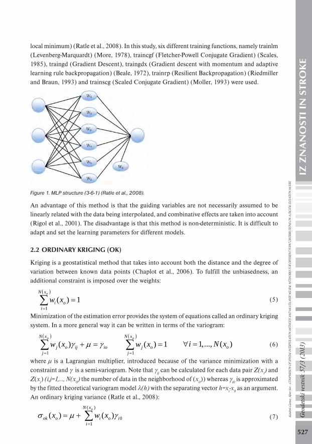
local minimum) (Ratle et al., 2008). In this study, six different training functions, namely trainlm (Levenberg-Marquardt) (More, 1978), traincgf (Fletcher-Powell Conjugate Gradient) (Scales, 1985), traingd (Gradient Descent), traingdx (Gradient descent with momentum and adaptive learning rule backpropagation) (Beale, 1972), trainrp (Resilient Backpropagation) (Riedmiller and Braun, 1993) and trainscg (Scaled Conjugate Gradient) (Moller, 1993) were used.

Figure 1. MLP structure (3-6-1) (Ratle et al., 2008).

An advantage of this method is that the guiding variables are not necessarily assumed to be linearly related with the data being interpolated, and combinative effects are taken into account (Rigol et al., 2001). The disadvantage is that this method is non-deterministic. It is difficult to adapt and set the learning parameters for different models.

2.2 ORDINARY KRIGING (OK)

Kriging is a geostatistical method that takes into account both the distance and the degree of variation between known data points (Chaplot et al., 2006). To fulfill the unbiasedness, an additional constraint is imposed over the weights:

oxN

ioi xw

11)(   (5)

Minimization of the estimation error provides the system of equations called an ordinary kriging system. In a more general way it can be written in terms of the variogram:

oxN

jioijoj xw

1)(

oxN

joj xw

11)( )(,.......,1 oxNi   1,..., ( )oi N x∀ = (6)

where µ is a Lagrangian multiplier, introduced because of the variance minimization with a constraint and γ is a semi-variogram. Note that γ

ij can be calculated for each data pair Z(x

i) and

Z(xj) (i,j=1,…, N(x

0) the number of data in the neighborhood of (x

0)) whereas γ

i0 is approximated

by the fitted theoretical variogram model λ(h) with the separating vector h=xi-x

0 as an argument.

An ordinary kriging variance (Ratle et al., 2008):

)(

10)()(

oxN

iioiook xwx   (7) Ku

talmi

s Gum

us, A

lper S

en -

COM

PARI

SON

OF SP

ATIA

L INT

ERPO

LATIO

N M

ETHO

DS A

ND M

ULTI-

LAYE

R NEU

RAL N

ETW

ORKS

FOR D

IFFER

ENT P

OINT

DIST

RIBU

TIONS

ON

A DI

GITA

L ELE

VATIO

N M

ODEL

528

Geo

dets

ki v

estn

ik 5

7/3

(201

3)IZ

ZN

AN

OST

I IN

STR

OK

E

The advantage of this method is the statistical formulation of the best linear unbiased estimate. The disadvantage is that the weights must be computed for each node of the grid, that is why this method is used for small samples, and the method produces undesirable “pits” and “circular” contours (Dressler, 2009).

2.3 INVERSE DISTANCE WEIGHTED (IDW)

The simplest form of IDW interpolation is called the Shepard’s method (Shepard, 1968).

n

iii fwyxF

1),(   (8)

where n is the number of distributed points in the data set, fi are the function values at the

distributed points and wi are the weight functions assigned to each point. The influence of a

known data point is inversely related to the distance from the unknown location that is being estimated. Shepard (1968) used weight function:

n

j

pj

pii ddw

0/   (9)

where p is an arbitrary positive real number called the power parameter (typically p = 2), dj are

the distances from the dispersion points to the interpolation point:

22 )()( iii yyxxd   (10)

where (x, y) are coordinates of the interpolation point and (xi, y

i) are the coordinates of each

dispersion point. The weight functions are normalized as a sum of the weights of the unit (Azpurua and Ramos, 2010).

Although IDW is simply implemented, high computer time is needed if the number of points is large due to the computation of distances, and has the tendency to generate "bull's-eye" patterns of concentric contours (Dressler, 2009).

2.4 MODIFIED SHEPARD’S METHOD (MS)

The Modified Shepard's Method uses an inverse distance weighted least squares method. The Modified Shepard's Method can be either an exact or a smoothing interpolator. Franke and Nielson (1980) developed a modification that eliminates the insufficiency of the Shepard’s method, and does not tend to generate "bull's eye" patterns.

As detailed in Basso et al. (1999), the first step in this method is the definition of the radii of influence, R

q and R

w. While R

q denotes the radius of influence of the data points in the nodal

functions, Rw denotes the radius of influence of the nodal functions in the interpolant.

( / 2) /q qR D N N=

NNDR gq /)2/( NNDR ww /)2/(   (11)

where D = maxi,j d

i (x

j,y

j), N is the total number of data points. The values of N

q and N

w can

be interpreted as representing the number of data points estimated to lie within the circles Kutal

mis G

umus

, Alpe

r Sen

- CO

MPA

RISO

N OF

SPAT

IAL I

NTER

POLA

TION

MET

HODS

AND

MUL

TI-LA

YER N

EURA

L NET

WOR

KS FO

R DIFF

EREN

T POI

NT D

ISTRI

BUTIO

NS O

N A

DIGI

TAL E

LEVA

TION

MOD

EL

529

Geo

dets

ki v

estn

ik 5

7/3

(201

3)IZ

ZN

AN

OST

I IN

STR

OK

E

of radii Rq and R

w respectively. After calculating the radii R

q and R

w, the nodal functions are

computed using the least squares method. These functions are calculated based only on data points sampled inside radius R

q. This slight modification gives a local behavior to the method.

The distance function ρi:

1/ ρi (x

iy) = (R

q –

d

i)/R

q d

i (12)

(Rq –

d

i) denotes the positive part of the quantity. The next step is to solve (for each nodal point

(xk,y

k), k=1, … , N) the least squares problem. The Modified Shepard formula:

)),(/1/()),(/),((),(1

2

1

2

N

kk

N

kkk yxVyxVyxQyxfD   (13)

where Qk(x,y)

is the nodal functions.

Each grid point is calculated based on the nodal functions computed for the sampled points inside a circle of radius R

w. This is defined by the Equation (13).

1/Vk(x, y) = (R

w –

d

k)/R

w d

k (14)

2.5 TRIANGULATION WITH LINEAR INTERPOLATION METHOD (TWL)

In the Triangulated Irregular Network (TIN) model, a finite set of points is stored together with their elevation. The points need not lie in any particular pattern, and the density may vary. On these points a planar triangulation is given based on a Delaunay’s triangulation. Any point in the domain will lie on a vertex, an edge or in a triangle of the triangulation. If the point does not lie on a vertex, then its elevation is obtained by linear interpolation (Kreveld, 2000). Suppose T is a DEM point in triangle abc. Under the assumption that the triangle vertices are error-free, TIN interpolation can be written as (Hu et al., 2009)

HT = w

aH

a + w

bH

b + w

cH

c ,

w

a + w

b + w

c = 1, w

a , w

b , w

c > 0 (15)

where H is the height, wa , w

b , w

c are the areal proportions of the sub-triangles constructed using

T. If s is the total area of triangle abc, sa , s

b , s

c are the areas of the sub-triangles, then

wa = s

a /s, w

b = s

b /s, w

c = s

c /s (16)

The TWL is very fast, but it is limited to the convex envelope of the points, resulting surface is not smooth and the division into triangles may be ambiguous, and requires a medium-large number of data point to generate acceptable results (Dressler, 2009).

2.6 MULTIQUADRIC RADIAL BASIS FUNCTION (MRBF)

Hardy (1968) introduced the multiquadric method for the construction of approximate two-dimensional surfaces of field data. The method of radial basis functions uses the interpolation function in the given form:

n

iiii YXyxwyxpyxf

1),(),(.),(),(   (17)

Kutal

mis G

umus

, Alpe

r Sen

- CO

MPA

RISO

N OF

SPAT

IAL I

NTER

POLA

TION

MET

HODS

AND

MUL

TI-LA

YER N

EURA

L NET

WOR

KS FO

R DIFF

EREN

T POI

NT D

ISTRI

BUTIO

NS O

N A

DIGI

TAL E

LEVA

TION

MOD

EL

530

Geo

dets

ki v

estn

ik 5

7/3

(201

3)IZ

ZN

AN

OST

I IN

STR

OK

E

where p(x, y) is a polynomial, wi∈R are real weights, is the Euclidean distance between points

(x, y) and (Xi, Y

i), is a radial basis function. A commonly used multiquadric radial basis function

is given in Table 2. (r, is the anisotropically rescaled, relative distance from the point to the node; c, is the smoothing parameter):

Radial Basis Function ( )(r ) Equation

Multiquadric 22 cr

Inverse Multiquadric 22/1 cr

Multilog )log( 22 cr

Natural Cubic Spline 2/322 )( cr

Thin Plate Spline )log()( 2222 crcr

 Table 2. Types of radial basis function.

The interpolation process starts with polynomial regression using the polynomial p(x, y). Then the following system of n linear equations is solved for unknown weights w

i, (i=1,…,n)

determined by imposing the interpolation conditions, which lead to a symmetric system of linear equations. The Lagrangian form is an easy evaluation of linear equations.

njYXYXwYXpZn

iiijjijjj ....,,1,,,.),(

1

  (18)

As soon as the weights (wi) are determined, the z-value of the surface can be directly computed

from Equation (17) at any point.

The advantages of this method are that the system of linear equations has to be solved only once in contrast to the Kriging method, where to be solved for each grid node, and uses a range of kernel functions. The disadvantages are that if the number of points n is large, the number of linear equations is also large, moreover, the matrix of the system is not sparse, which leads to a long computational time and possibly to the propagation of rounding errors (Dressler, 2009).

3 STUDY AREA

USGS National Elevation Dataset (NED) 1/3 arc-second (approximately 10 meters grid spacing) DEM was used in this study. The dataset has been tested by comparing it with a reference data which are the geodetic control points that the National Geodetic Survey uses for gravity and geoid modeling. The NED value at each of the control point locations was derived through bilinear interpolation, and error statistics were calculated. Bilinear interpolation is the calculation of the new pixel value performed by the weight of the four surrounding pixels (Hu et al., 2009). The production method is an improved contour-to-grid interpolation known as “LineTrace+” (LT4X) (Osborn et al., 2001). The overall absolute vertical accuracy expressed as RMSE for LT4X production is 2.17 m (Gesch, 2007).

The study area is Lower Beaver in Colorado, USA. The difference between maximum and minimum elevations (the relief) is 82 m in the study area. The horizontal datum is the North Ku

talmi

s Gum

us, A

lper S

en -

COM

PARI

SON

OF SP

ATIA

L INT

ERPO

LATIO

N M

ETHO

DS A

ND M

ULTI-

LAYE

R NEU

RAL N

ETW

ORKS

FOR D

IFFER

ENT P

OINT

DIST

RIBU

TIONS

ON

A DI

GITA

L ELE

VATIO

N M

ODEL

531

Geo

dets

ki v

estn

ik 5

7/3

(201

3)IZ

ZN

AN

OST

I IN

STR

OK

E

American Datum of 1983 and UTM zone is 12N. The lower left corner coordinates of DEM are (ϕ: 38° 44' 16.8''; λ: -112° 38' 45.6'') and the upper right corner coordinates are (ϕ: 38° 45' 25.2''; λ: -112° 37' 22.8''). The study area is 2-by-2 square kilometers. The 3D model of the study area is shown in Figure 2.

Figure 2. 3D model of the study area.

4 DATA PREPROCESSING

Depressions of a DEM may be natural reflections of the terrain, or the artificial depressions as a result of interpolation methods, input data errors, or restrictions in DEM resolution. Sinks are often errors due to the resolution of the data or rounding of elevations to the nearest integer value. In this study, hydrology tool of ArcGIS 10 software was utilized. The depressions were removed by rising to the lowest elevation value on the rim of the depression (Jenson and Domingue, 1988) for improving DEM. Filling sinks modifies the elevation value to eliminate the problems about cells surrounded with higher elevation and resumes the water flow. Sinks were filled based on appropriate the z-limit (in this study, 16 cm). The z-limit specifies the maximum depth of a sink that will be filled. A procedure using geoprocessing tools to find z-limit for the “Fill” as follows (ArcGIS 10 Help).

• Use “Sink” to create a raster of sinks coded with depth.

• Use “Watershed” to create a raster of the contributing area for each sink.

• Use “Zonal Statistics” with the minimum statistic to create a raster of the minimum elevation in the watershed of each sink.

• Use “Zonal Fill” to create a raster of the maximum elevation in the watershed of each sink.

• Use “Minus” to subtract the minimum value from the maximum value to find the depth.

For the neural network implementation, all of the input data were normalized based on minimum-maximum normalization to avoid the numerical conflicting. Minimum-maximum normalization (Han et al., 2012): Ku

talmi

s Gum

us, A

lper S

en -

COM

PARI

SON

OF SP

ATIA

L INT

ERPO

LATIO

N M

ETHO

DS A

ND M

ULTI-

LAYE

R NEU

RAL N

ETW

ORKS

FOR D

IFFER

ENT P

OINT

DIST

RIBU

TIONS

ON

A DI

GITA

L ELE

VATIO

N M

ODEL

532

Geo

dets

ki v

estn

ik 5

7/3

(201

3)IZ

ZN

AN

OST

I IN

STR

OK

E

minmax

min'

xxxxX i

i

  (19)

where xmin

and xmax

are the minimum and maximum values of X coordinate in the dataset, respectively. X

i is normalized based on the range of the data (likewise, Y coordinate).

5 POINT DISTRIBUTION

In predicting height, different point distributions were compared such as curvature, grid, random and uniform on the DEM. Grid distribution decreases the number of points in an irregular point space, not considering curvature and original density of pattern. However, curvature distribution decreases the number of points on surfaces of which height is closely similar but maintains details in high curved areas. Uniform distribution decreases the number of points uniformly on surfaces of which height is closely similar, but reduces the number of points on curved surfaces to a specified density. Random distribution removes a percentage of points randomly from an irregular point space.

Figure 3. Study area with contours and four different point distributions in the red rectangular.

In this study, totally 47,089 points obtained from DEM were used. As a result of using grid, random, uniform and curvature distributions, the number of points was reduced by 50%, e.g. Ku

talmi

s Gum

us, A

lper S

en -

COM

PARI

SON

OF SP

ATIA

L INT

ERPO

LATIO

N M

ETHO

DS A

ND M

ULTI-

LAYE

R NEU

RAL N

ETW

ORKS

FOR D

IFFER

ENT P

OINT

DIST

RIBU

TIONS

ON

A DI

GITA

L ELE

VATIO

N M

ODEL

533

Geo

dets

ki v

estn

ik 5

7/3

(201

3)IZ

ZN

AN

OST

I IN

STR

OK

E

more points were selected on the characteristic parts of surface, while fewer points were used on the flat parts in the curvature distribution. Different point distributions in the interpolation methods and ANN prediction were used for comparing the effect of different sampling densities (in this case, 100% and 50%) and the topographic variability. Besides, the characteristic lines (ridges and valleys) could contribute to the point distribution. In Figure 3, four different point distributions (only shown in the red rectangular as an example) are represented with contours of the study area obtained from the DEM. It is realized that the curvature distribution maintains more points among dense contours (highly curved) than flat areas.

6 EXPERIMENTATION

In this study, MLP was applied by Matlab R2009b neural network toolbox and interpolation methods were performed by Surfer 9.0. When training multilayer networks, the general practice is to first divide the data into three subsets. The first subset is the training set, which is used for computing the gradient and updating the network weights and biases. The second subset is the validation set. The error in the validation set is monitored during the training process. The validation error normally decreases during the initial phase of training, as does the training set error. However, when the network begins to overfit the data, the error in the validation set typically begins to rise. The test set error is not used during training but it is used to compare different models. Test error is not minimized and thus not propagated backwards from the MLP outputs to the input. The size of the test can range between 1-25% of the total amount of data available (Ratle et al., 2008). In this study, ratios for training, testing and validation were 0.7, 0.15 and 0.15, respectively.

Before training MLP, the weights and biases are initialized. The process of training a neural network involves tuning the values of the weights and biases of the network to optimize network performance, as defined by the network performance function which is the Root Mean Square Error (RMSE) as defined in Equation (18).

N

iii ZZ

NRMSE

1

2)'(1  (20)

where Zi’ is the network output height, Z

i is the target output height.

In neural network toolbox, the magnitude of the gradient and the number of validation checks are used to terminate the training. The gradient will become very small as the training reaches a minimum of the performance. The number of validation checks represents the number of successive iterations that the validation performance fails to decrease.

In this study, the X-Y coordinates were the input, while the Z coordinates were the output. The parameters of the multi-layer neural network were experimentally determined by approximately 70 variations. Six different training functions, namely trainlm, traincgf, traingd, traingdx, trainrp, and trainscg, and different hidden layer and neuron numbers and epochs were examined. The best variations are given in Table 3. The best performance was performed by the Levenberg-Marquardt (trainlm) function based on RMSE within the range of 12 cm and 16 cm that changed Ku

talmi

s Gum

us, A

lper S

en -

COM

PARI

SON

OF SP

ATIA

L INT

ERPO

LATIO

N M

ETHO

DS A

ND M

ULTI-

LAYE

R NEU

RAL N

ETW

ORKS

FOR D

IFFER

ENT P

OINT

DIST

RIBU

TIONS

ON

A DI

GITA

L ELE

VATIO

N M

ODEL

534

Geo

dets

ki v

estn

ik 5

7/3

(201

3)IZ

ZN

AN

OST

I IN

STR

OK

E

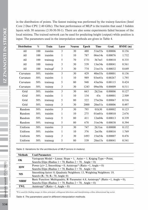
in the distribution of points. The fastest training was performed by the trainrp function (Intel Core 2 Duo CPU 2.40 GHz). The best performance of MLP is the trainlm that used 3 hidden layers with 30 neurons (2-30-30-30-1). There are also some experiments failed because of the local minima. The trained network can be used for predicting height (output) while position is input. The parameters used in the interpolation methods are given in Table 4.

Distribution % Train Layer Neuron Epoch Time Grad. RMSE (m)

All 100 trainlm 3 30 480 51m55s 0.00006 0.156

All 100 trainlm 1 10 787 06m14s 0.00076 1.732

All 100 trainscg 5 70 1731 3h7m5 0.00018 0.335

All 100 trainrp 3 30 539 13m34s 0.00041 0.561

All 100 traincgf 3 30 774 21m15s 0.00032 0.649

Curvature 50% trainlm 3 30 429 40m55s 0.00001 0.136

Curvature 50% trainlm 1 10 989 03m41s 0.00267 1.795

Curvature 50% trainscg 5 80 948 43m56s 0.00115 0.424

Curvature 50% trainrp 3 30 1243 09m50s 0.00009 0.511

Grid 50% trainlm 3 30 663 2h21m 0.00006 0.127

Grid 50% trainlm 1 10 134 43s 0.00001 2.509

Grid 50% trainscg 5 80 522 27m26s 0.00067 0.516

Grid 50% trainrp 3 30 2000 20m51s 0.00006 0.497

Random 50% trainlm 3 30 795 01h30 0.00002 0.123

Random 50% trainlm 1 10 275 01m01s 0.00010 2.676

Random 50% trainrp 5 80 411 12m04s 0.00013 0.339

Random 50% trainscg 5 80 678 31m34s 0.00038 0.394

Uniform 50% trainlm 3 30 747 2h31m 0.00000 0.132

Uniform 50% trainlm 1 10 376 2m10s 0.00016 1.769

Uniform 50% trainrp 3 30 1493 15m54s 0.00007 0.476

Uniform 50% trainscg 5 80 539 28m15s 0.00041 0.541

 Table 3. Variations for the architecture of MLP (errors in meters).

Methods Used Parameters

OK Variogram Model = Linear, Slope = 1, Aniso = 1, Kriging Type = Point, Searchs Elips (Radius 1 = 70, Radius 2 = 70, Angle = 0)

IDW Power (p)= 2, Smoothing = 0, Anistropy* (Ratio =1, Angle = 0) Searchs Elips (Radius 1 = 70, Radius 2 = 70, Angle = 0)

MS Smoothing factor: 0, Quadratic Neighbors: 13, Weighting Neighbors: 19, Search (Rq: 70, Rw: 70, Angle: 0)

MRBF Basic Function: Multiquadric, R2 Parameter: 6.8, Anistropy* (Ratio =1, Angle = 0), Searchs Elips (Radius 1 = 70, Radius 2 = 70, Angle = 0)

TWL Anistropy* (Ratio =1, Angle = 0)

 *It is used for finding ranges in three principal, orthogonal directions and transforming a three dimensional lag vector.

Table 4. The parameters used in different interpolation methods.Kutal

mis G

umus

, Alpe

r Sen

- CO

MPA

RISO

N OF

SPAT

IAL I

NTER

POLA

TION

MET

HODS

AND

MUL

TI-LA

YER N

EURA

L NET

WOR

KS FO

R DIFF

EREN

T POI

NT D

ISTRI

BUTIO

NS O

N A

DIGI

TAL E

LEVA

TION

MOD

EL

535

Geo

dets

ki v

estn

ik 5

7/3

(201

3)IZ

ZN

AN

OST

I IN

STR

OK

E

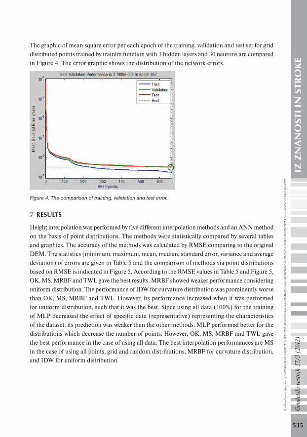
The graphic of mean square error per each epoch of the training, validation and test set for grid distributed points trained by trainlm function with 3 hidden layers and 30 neurons are compared in Figure 4. The error graphic shows the distribution of the network errors.

Figure 4. The comparison of training, validation and test error.

7 RESULTS

Height interpolation was performed by five different interpolation methods and an ANN method on the basis of point distributions. The methods were statistically compared by several tables and graphics. The accuracy of the methods was calculated by RMSE comparing to the original DEM. The statistics (minimum, maximum, mean, median, standard error, variance and average deviation) of errors are given in Table 5 and the comparison of methods via point distributions based on RMSE is indicated in Figure 5. According to the RMSE values in Table 5 and Figure 5, OK, MS, MRBF and TWL gave the best results. MRBF showed weaker performance considering uniform distribution. The performance of IDW for curvature distribution was prominently worse than OK, MS, MRBF and TWL. However, its performance increased when it was performed for uniform distribution, such that it was the best. Since using all data (100%) for the training of MLP decreased the effect of specific data (representative) representing the characteristics of the dataset, its prediction was weaker than the other methods. MLP performed better for the distributions which decrease the number of points. However, OK, MS, MRBF and TWL gave the best performance in the case of using all data. The best interpolation performances are MS in the case of using all points, grid and random distributions; MRBF for curvature distribution, and IDW for uniform distribution.

Kutal

mis G

umus

, Alpe

r Sen

- CO

MPA

RISO

N OF

SPAT

IAL I

NTER

POLA

TION

MET

HODS

AND

MUL

TI-LA

YER N

EURA

L NET

WOR

KS FO

R DIFF

EREN

T POI

NT D

ISTRI

BUTIO

NS O

N A

DIGI

TAL E

LEVA

TION

MOD

EL

536

Geo

dets

ki v

estn

ik 5

7/3

(201

3)IZ

ZN

AN

OST

I IN

STR

OK

E

50% Ordinary Kriging Modified Shepard's Inverse Distance Weighted

Dist. Cur. Grid Rand. Uni. Cur. Grid Rand. Uni. Cur. Grid Rand. Uni.

Min. -1.268 -1.417 -1.615 -1.671 -1.458 -1.660 -1.172 -1.937 -2.104 -2.059 -1.472 -1.617

Max. 2.139 1.828 1.931 2.225 2.758 1.574 2.263 1.934 2.522 1.894 3.802 1.581

Mean 0.001 0.001 0.001 0.001 0.000 0.000 0.000 0.000 0.002 0.000 0.001 0.000

Median 0.000 0.000 0.000 0.000 0.000 0.000 0.000 0.000 0.000 0.000 0.000 0.000

Standard error 0.000 0.000 0.000 0.000 0.000 0.000 0.000 0.000 0.001 0.000 0.000 0.000

Variance 0.005 0.008 0.006 0.007 0.007 0.005 0.005 0.008 0.020 0.007 0.009 0.005

Average deviation 0.034 0.037 0.031 0.038 0.036 0.030 0.032 0.038 0.062 0.035 0.038 0.028

RMSE 0.074 0.087 0.075 0.086 0.084 0.073 0.072 0.092 0.142 0.082 0.097 0.069

50% Multiq. Radial Basis Function Triangulation with Linear Multi-Layer Perceptron

Dist. Cur. Grid Rand. Uni. Cur. Grid Rand. Uni. Cur. Grid Rand. Uni.

Min. -1.171 -1.458 -1.933 -1.504 -1.671 -2.012 -1.309 -1.952 -1.970 -1.851 -2.736 -2.384

Max. 2.261 2.758 1.973 2.428 2.225 2.015 1.872 1.887 2.260 1.275 1.490 1.692

Mean 0.000 0.000 0.000 0.002 0.001 0.000 0.001 0.001 0.000 -0.002 0.000 -0.000

Median 0.000 0.000 0.000 0.000 0.000 0.000 0.000 0.000 -0.000 -0.001 0.000 0.000

Standard error 0.000 0.000 0.000 0.000 0.000 0.000 0.000 0.000 0.001 0.001 0.001 0.001

Variance 0.005 0.007 0.006 0.010 0.007 0.007 0.007 0.008 0.018 0.016 0.015 0.017

Average deviation 0.032 0.036 0.033 0.041 0.038 0.036 0.034 0.036 0.090 0.085 0.082 0.086

RMSE 0.071 0.084 0.078 0.102 0.086 0.085 0.082 0.087 0.136 0.127 0.123 0.132

100% Ordinary Kriging Modified Shepard's Inverse Distance Weighted

Min. -0.737 -1.838 -1.495

Max. 1.253 1.554 2.797

Mean 0.000 0.000 0.001

Median 0.000 0.000 0.000

Standard error 0.000 0.000 0.000

Variance 0.001 0.001 0.006

Average deviation 0.011 0.008 0.022

RMSE 0.038 0.034 0.080

100% Multiq. Radial Basis Function Triangulation with Linear Multi-Layer Perceptron

Min. -0.756 -0.917 -2.915

Max. 1.226 1.649 4.147

Mean 0.000 0.001 -0.003

Median 0.000 0.000 0.000

Standard error 0.000 0.000 0.000

Variance 0.001 0.002 0.024

Average deviation 0.009 0.013 0.001

RMSE 0.035 0.046 0.156

 Table 5. The statistical results of error (in meters) via point distributions for height interpolation. Ku

talmi

s Gum

us, A

lper S

en -

COM

PARI

SON

OF SP

ATIA

L INT

ERPO

LATIO

N M

ETHO

DS A

ND M

ULTI-

LAYE

R NEU

RAL N

ETW

ORKS

FOR D

IFFER

ENT P

OINT

DIST

RIBU

TIONS

ON

A DI

GITA

L ELE

VATIO

N M

ODEL

537

Geo

dets

ki v

estn

ik 5

7/3

(201

3)IZ

ZN

AN

OST

I IN

STR

OK

E

Figure 5. Graphic of performances (RMSE) for each method using different point distributions.

The contours were obtained for visualizing the interpolated surface by different methods. Using all data (100%) for MLP training yielded weak prediction results. Therefore, MLP simplified the contours. For example, the eliminated details of the contour lines, as an MLP result compared with other interpolation results in the case of using all data, are shown by red circle in Figure 6.

Figure 6. The contours obtained by interpolation methods and MLP for each point distribution and eliminated details of contours in red circles.

In addition to these results, three different cross-sections on the characteristic parts of the surface were selected and analyzed in order to determine the effect of methods using all data (100%). A-B, C-D and E-F cross- sections are shown on the 3D model and the contours in Figure 7. The A-B cross-section is beveled and E-F is more rugged than the C-D cross-section. The methods were examined based on RMSE for 588, 1500 and 522 points on the A-B, C-D and E-F cross-sections, respectively. The RMSE results of the interpolations are given in Table 6. A graphic of performances of each method via point distributions based on RMSE for each cross-section is given in Figure 8. Ku

talmi

s Gum

us, A

lper S

en -

COM

PARI

SON

OF SP

ATIA

L INT

ERPO

LATIO

N M

ETHO

DS A

ND M

ULTI-

LAYE

R NEU

RAL N

ETW

ORKS

FOR D

IFFER

ENT P

OINT

DIST

RIBU

TIONS

ON

A DI

GITA

L ELE

VATIO

N M

ODEL

538

Geo

dets

ki v

estn

ik 5

7/3

(201

3)IZ

ZN

AN

OST

I IN

STR

OK

E

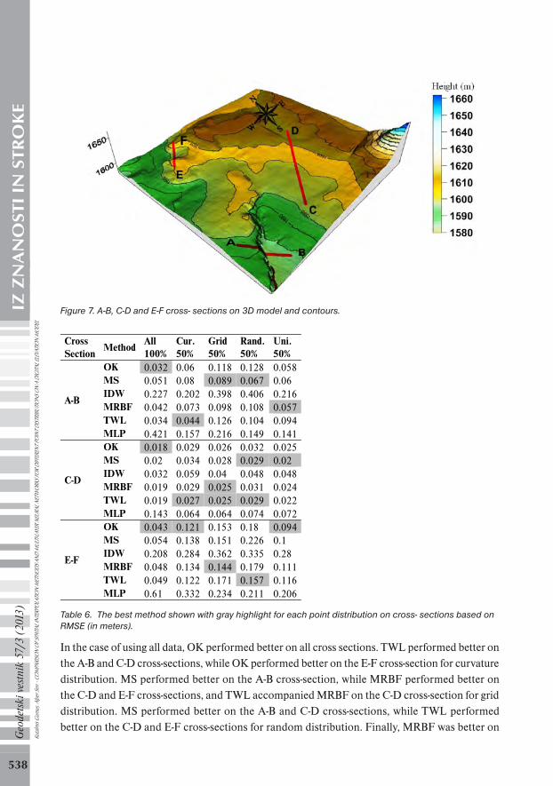
Figure 7. A-B, C-D and E-F cross- sections on 3D model and contours.

Cross Method

All 100%

Cur. Grid Rand. Uni. Section 50% 50% 50% 50%

A-B

OK 0.032 0.06 0.118 0.128 0.058MS 0.051 0.08 0.089 0.067 0.06 IDW 0.227 0.202 0.398 0.406 0.216MRBF 0.042 0.073 0.098 0.108 0.057TWL 0.034 0.044 0.126 0.104 0.094MLP 0.421 0.157 0.216 0.149 0.141

C-D

OK 0.018 0.029 0.026 0.032 0.025MS 0.02 0.034 0.028 0.029 0.02 IDW 0.032 0.059 0.04 0.048 0.048MRBF 0.019 0.029 0.025 0.031 0.024TWL 0.019 0.027 0.025 0.029 0.022MLP 0.143 0.064 0.064 0.074 0.072

E-F

OK 0.043 0.121 0.153 0.18 0.094MS 0.054 0.138 0.151 0.226 0.1 IDW 0.208 0.284 0.362 0.335 0.28 MRBF 0.048 0.134 0.144 0.179 0.111TWL 0.049 0.122 0.171 0.157 0.116MLP 0.61 0.332 0.234 0.211 0.206

 Table 6. The best method shown with gray highlight for each point distribution on cross- sections based on RMSE (in meters).

In the case of using all data, OK performed better on all cross sections. TWL performed better on the A-B and C-D cross-sections, while OK performed better on the E-F cross-section for curvature distribution. MS performed better on the A-B cross-section, while MRBF performed better on the C-D and E-F cross-sections, and TWL accompanied MRBF on the C-D cross-section for grid distribution. MS performed better on the A-B and C-D cross-sections, while TWL performed better on the C-D and E-F cross-sections for random distribution. Finally, MRBF was better on

Kutal

mis G

umus

, Alpe

r Sen

- CO

MPA

RISO

N OF

SPAT

IAL I

NTER

POLA

TION

MET

HODS

AND

MUL

TI-LA

YER N

EURA

L NET

WOR

KS FO

R DIFF

EREN

T POI

NT D

ISTRI

BUTIO

NS O

N A

DIGI

TAL E

LEVA

TION

MOD

EL

539

Geo

dets

ki v

estn

ik 5

7/3

(201

3)IZ

ZN

AN

OST

I IN

STR

OK

E

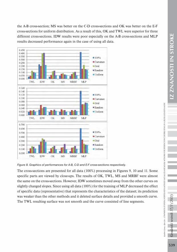
the A-B cross-section; MS was better on the C-D cross-sections and OK was better on the E-F cross-sections for uniform distribution. As a result of this, OK and TWL were superior for three different cross-sections. IDW results were poor especially on the A-B cross-sections and MLP results decreased performance again in the case of using all data.

Figure 8. Graphics of performances for A-B, C-D and E-F cross-sections respectively.

The cross-sections are presented for all data (100%) processing in Figures 9, 10 and 11. Some specific parts are viewed by close-ups. The results of OK, TWL, MS and MRBF were almost the same on the cross-sections. However, IDW sometimes moved away from the other curves on slightly changed slopes. Since using all data (100%) for the training of MLP decreased the effect of specific data (representative) that represents the characteristics of the dataset; its prediction was weaker than the other methods and it deleted surface details and provided a smooth curve. The TWL resulting surface was not smooth and the curve consisted of line segments.

Kutal

mis G

umus

, Alpe

r Sen

- CO

MPA

RISO

N OF

SPAT

IAL I

NTER

POLA

TION

MET

HODS

AND

MUL

TI-LA

YER N

EURA

L NET

WOR

KS FO

R DIFF

EREN

T POI

NT D

ISTRI

BUTIO

NS O

N A

DIGI

TAL E

LEVA

TION

MOD

EL

540

Geo

dets

ki v

estn

ik 5

7/3

(201

3)IZ

ZN

AN

OST

I IN

STR

OK

E

Figure 9. The views of the specific parts of A-B cross- section obtained different interpolation methods (TWL, IDW, OK, MS, MRBF, respectively) and ANN (MLP).

Figure 10. The views of the specific parts of C-D cross- section obtained different interpolation methods (TWL, IDW, OK, MS, MRBF, respectively) and ANN (MLP).

Figure 11. The views of the specific parts of E-F cross- section obtained different interpolation methods (TWL, IDW, OK, MS, MRBF, respectively) and ANN (MLP).Ku

talmi

s Gum

us, A

lper S

en -

COM

PARI

SON

OF SP

ATIA

L INT

ERPO

LATIO

N M

ETHO

DS A

ND M

ULTI-

LAYE

R NEU

RAL N

ETW

ORKS

FOR D

IFFER

ENT P

OINT

DIST

RIBU

TIONS

ON

A DI

GITA

L ELE

VATIO

N M

ODEL

541

Geo

dets

ki v

estn

ik 5

7/3

(201

3)IZ

ZN

AN

OST

I IN

STR

OK

E

8 CONCLUSIONS

In this study, the authors determined the accuracy of interpolation methods and an artificial neural network in predicting the height of different point distributions on a Digital Elevation Model (DEM). This study also aims to quantify the effects of topographic variability and sampling density. Errors of different interpolations and ANN prediction were evaluated for different point distributions and three different cross-sections on the characteristic parts of the surface were selected and analyzed. Generally, OK, MS, MRBF and TWL gave promising results based on RMSE and were more effective in terms of reflecting the characteristics of the surface. Although MLP simplified the contours, it was a satisfactory predictor for curvature, grid, random and uniform distributions. An advantage of ANN is that the guiding variables are not necessarily assumed to be linearly related with the data being interpolated, and combinative effects are taken into account. However, ANN is a non-deterministic method and it requires so many experiments. The best interpolation performances are MS in the case of using all points, grid and random distributions; MRBF for curvature distribution, and IDW for uniform distribution. Since the RMSE is a statistical value, it could not give enough information about the characteristic parts of topography (e.g. ridges, valleys, peaks, pits etc.). Therefore, the cross-sections on the characteristic parts were visualized and evaluated. However, it would be useful to prove the tested interpolation methods by means of geovisual methods. In the analysis of different cross-sections on the characteristic parts of the surface, OK and TWL were superior for three different cross-sections. In the future, DEMs for topographically different terrains (e.g. flat, hilly and mountainous) will be evaluated with several training functions of MLP.

ACKNOWLEDGEMENTS

The authors would like to thank the referees for their careful review and Assoc. Prof. Dr. Turkay Gokgoz, Yildiz Technical University, Geomatic Engineering Dep., for the valuable comments.

Literature and reference: ArcGIS 10 Help: http://help.arcgis.com/en/arcgisdesktop/10.0/help.

Attorre, F., Alfo, M., Sanctis, M. D., Francesconi, F., Bruno, F. (2007). Comparison of interpolation methods for mapping climatic and bioclimatic variables at regional scale. International Journal of Climatology, 27 (13), 1825-1843, (ISSN)1097-0088doi:10.1002/joc.

Azpurua, M,. Ramos, K.D. (2010). A comparison of spatial interpolation methods for estimation of average electromagnetic field magnitude. Progress In Electromagnetics Research M, Vol. 14, 135-145.

Basso, K., Zingano, P. R. Á., Freitas, C. M. D. S. (1999). Interpolation of scattered data: investigating alternatives for the modified shepard method. In: Proceedings Of Sibgrapi 99. - Xii Brazilian Symposium On Computer Graphics And Image Processing, 39-47.

Beale, E.M.L., (1972). A derivation of conjugate gradients. in F.A. Lootsma, Ed. Numerical methods for nonlinear optimization. London:Academic Press.

Chaplot, V., Darboux, F., Bourennane, H., Leguédois, S., Silvera, N., Phachomphon, K. (2006). Accuracy of interpolation techniques for the derivation of digital elevation models in relation to landform types and data density. Geomorphology, 77(1-2), 126–141. doi:10.1016/j.geomorph.2005.12.010.

De, S.S., Chattopadhyay, G., Debnath, A. (2009). Artificial Neural Network – a Tool for Prediction of Monsoon Rainfall over North and South Assam in India. Bulg. J. Phys. 36, 55–67. Ku

talmi

s Gum

us, A

lper S

en -

COM

PARI

SON

OF SP

ATIA

L INT

ERPO

LATIO

N M

ETHO

DS A

ND M

ULTI-

LAYE

R NEU

RAL N

ETW

ORKS

FOR D

IFFER

ENT P

OINT

DIST

RIBU

TIONS

ON

A DI

GITA

L ELE

VATIO

N M

ODEL

542

Geo

dets

ki v

estn

ik 5

7/3

(201

3)IZ

ZN

AN

OST

I IN

STR

OK

E

Deligiorgi, D., Philippopoulos K. (2011). Spatial Interpolation Methodologies in Urban Air Pollution Modeling: Application for the Greater Area of Metropolitan Athens, Greece. Advanced Air Pollution, Farhad Nejadkoorki (Ed.), ISBN: 978-953-307-511-2, InTech, DOI: 10.5772/17734.

Dressler, M. (2009). Art of Surface Interpolation, e-book, http://m.dressler.sweb.cz/AOSIM.pdf.

Erxleben, J., Elder, K., Davis, R. (2002). Comparison of spatial interpolation methods for estimating snow distribution in the Colorado Rocky Mountains. Hydrol. Processes, 3649(August), 3627–3649. doi:10.1002/hyp.1239.

Franke, R., Nielson, G. (1980). Smooth Interpolation of Large Sets of Scattered Data. International Journal for Numerical Methods in Engineering, v. 15, 1980, 1691-1704.

Gesch, D.B.(2007). The National Elevation Dataset. Digital Elevation Model Technologies and Applications: The DEM Users Manual, Maune, D. (ed.), 2nd Edition, American Society for Photogrammetry and Remote Sensing, Bethesda, Maryland, 99-118.

Guo, Q., Li, W., Yu, H., Alvarez, O. (2010). Effects of Topographic Variability and Lidar Sampling Density on Several DEM Interpolation Methods. Photogrammetric Engineering & Remote Sensing, Vol. 76, No. 6, 1–12.

Hardy, R.L. (1990). Theory and Applications of the Multiquadric-biharmonic Method. Computers Math. With Applic, v 19, no. 8/9, 163-208.

Hu, P., Liu, X., Hu, H. (2009). Accuracy Assessment of Digital Elevation Models based on Approximation Theory. Photogrammetric Engineering and Remote Sensing, Vol. 75, No.1, 49-56.

Jenson, S. K. and Domingue, J. O. (1988). Extracting topographic structure from digital elevation data for geographic information system analysis, Photogramm. Eng. Rem. S., 54, 1593–1600.

Han, J., Kamber, M., Pei, J. (2012). Data mining Concepts and Techniques, Elsevier Inc. Third Edition..

Kreveld, M. (2000). Digital Elevation Models and TIN Algorithms. Chap. 3 of Algorithmic Foundations of Geographic Information Systems, Kreveld, M., Nievergelt, J., Roos, T., Widmayer, P. (eds.), Springer, 40-41.

Lam, N.S.N. (1983). Spatial Interpolation Methods: A Review. The American Cartographer, Vol. 10, No. 2, 129-149.

Moller, M.F. (1993). A scaled conjugate gradient algorithm for fast supervised learning. Neural Networks, Vol. 6, 525–533.

More, J.J. (1978), The Levenberg-Marquardt algorithm: Implementation and theory. Numerical Analysis, Lecture notes in Math., No. 630, Springer, Berlin 1978.

Myers, D. E., (1994). Spatial interpolation: An overview. Geoderma, 62, 17–28.

Osborn, K., List, J., Gesch, D.B., Crowe, J., Merrill, G., Constance, E., Mauck, J., Lund, C., Caruso, V., Kosovich, J. (2001). National Digital Elevation Program (NDEP). Chap. 4 of Digital elevation model technologies and applications—the DEM users manual, Maune, D. (ed.), American Society for Photogrammetry and Remote Sensing, Bethesda, Maryland, 83-120. (Also available online at http://topotools.cr.usgs.gov/pdfs/osb_eros-pub-bkc_asprs.2001.pdf.)

Ratle, F., Pozdnoukhov, A., Demyanov, V., Timonin, V., Savelieva E. (2008). Spatial Data Analysis and Mapping Using Machine Learning Algorithms. Advanced Mapping of Enviromental Data Geostatistics, Machine Learning and Bayesian Maximum Entropy, Mikhail Kanevski (ed.), ISTE ,Wiley.

Riedmiller, M., Braun, H. (1993). A Direct Adaptive Method for Faster Backpropagation Learning: The RPROP Algorithm. Proceedings of the IEEE International Conference on Neural Networks (ICNN), San Francisco. 586 – 591.

Rigol, J.P., Jarvis C.H., Stuart, N. (2001). Artificial neural networks as a tool for spatial interpolation. Int. Journal of Geographical Information Science, Volume 15, Issue 4, 323-343.

Scales, L.E. (1985). Introduction to Non-Linear Optimization, New York, Springer-Verlag.

Sen, A., Gumusay, M. U., Kavas A., Bulucu U. (2008). Programming an Artificial Neural Network Tool for Spatial Interpolation in GIS - A Case Study for Indoor Radio Wave Propagation of WLAN. Sensors (8), 5996–6014. doi:10.3390/s8095996.

Shepard, D. (1968). A Two Dimensional Interpolation Function for Irregularly Spaced Data. Proc. 23rd Nat. Conf. ACM, 517-523.

Shrivastava, G., Karmakar, S., Kowar, M.K., Guhathakurta, P. (2012). Application of Artificial Neural Networks in Weather Forecasting:A Comprehensive Literature Review. International Journal of Computer Applications, Vol. 51, No. 18, Foundation of Computer Science, New York, NY, USA, 17-29.Ku

talmi

s Gum

us, A

lper S

en -

COM

PARI

SON

OF SP

ATIA

L INT

ERPO

LATIO

N M

ETHO

DS A

ND M

ULTI-

LAYE

R NEU

RAL N

ETW

ORKS

FOR D

IFFER

ENT P

OINT

DIST

RIBU

TIONS

ON

A DI

GITA

L ELE

VATIO

N M

ODEL

543

Geo

dets

ki v

estn

ik 5

7/3

(201

3)IZ

ZN

AN

OST

I IN

STR

OK

E

Snell, S.E., Gopal, S., Kaufmann R.K. (2000). Spatial Interpolation of Surface Air Temperatures Using Artificial Neural Networks: Evaluating Their Use for Downscaling GCMs. Journal Of Climate, 13(5), 886-895.

Zhang. Y. (2010). Spatial Interpolation of meteorology monitoring data for western China using back-propagation artificial neural networks. Communications and Networking in China (CHINACOM), 5th International ICST Conference, Beijing / China.

Zimmerman, D., Pavlik, C., Ruggles, A., Armstrong, M. (1999). An experimental comparison of ordinary and universal kriging and inverse distance weighting. Mathematical Geology, 31, 375–390. doi:10.1023/A:1007586507433.

Received for publication: 28 January 2012

Received by: 23 April 2013

Kutalmis Gumus, Research Assistant

Yildiz Technical University

Civil Engineering Faculty, Geomatic Engineering Depatment,

Surveying Division

Davutpasa Street, Esenler, Istanbul - Turkey

E-mail: kgumus@yildiz.edu.tr

Alper Sen, Research Assistant

Yildiz Technical University

Civil Engineering Faculty, Geomatic Engineering Department,

Cartography Division

Davutpasa Street, Esenler, Istanbul - Turkey

E-mail: alpersen@yildiz.edu.tr Kutal

mis G

umus

, Alpe

r Sen

- CO

MPA

RISO

N OF

SPAT

IAL I

NTER

POLA

TION

MET

HODS

AND

MUL

TI-LA

YER N

EURA

L NET

WOR

KS FO

R DIFF

EREN

T POI

NT D

ISTRI

BUTIO

NS O

N A

DIGI

TAL E

LEVA

TION

MOD

EL