OMG 402 - Operations Management Spring 1997 CLASS 8: Process and Inventory Control (1) Harry...
26
OMG 402 - Operations Management Spring 1997 CLASS 8: Process and Inventory Control (1) Harry Groenevelt
-
Upload
howard-benson -
Category
Documents
-
view
215 -
download
0
Transcript of OMG 402 - Operations Management Spring 1997 CLASS 8: Process and Inventory Control (1) Harry...

OMG 402 - Operations ManagementSpring 1997
CLASS 8:
Process and Inventory Control (1)
Harry Groenevelt

March 1997 2
Agenda
• Introduction
• Production and cost: the EOQ
• Production and time: JIT
• Summary of Insights
March 1997 3
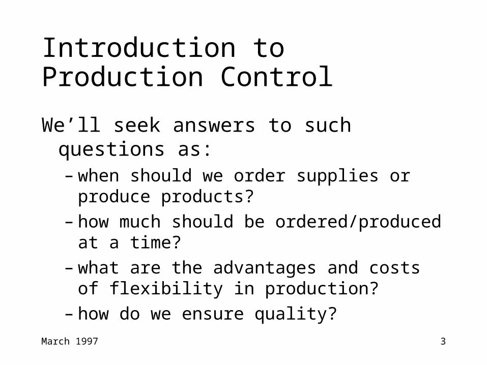
Introduction to Production Control
We’ll seek answers to such questions as:– when should we order supplies or produce
products?– how much should be ordered/produced at a
time?– what are the advantages and costs of flexibility
in production?– how do we ensure quality?
March 1997 4
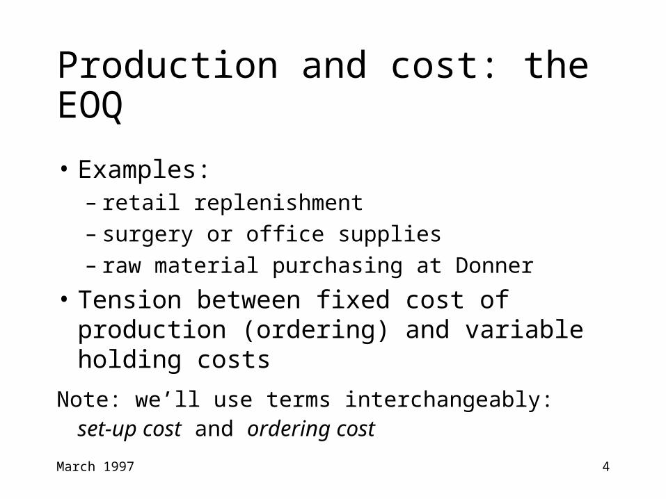
Production and cost: the EOQ
• Examples: – retail replenishment– surgery or office supplies– raw material purchasing at Donner
• Tension between fixed cost of production (ordering) and variable holding costs
Note: we’ll use terms interchangeably:set-up cost and ordering cost

March 1997 5ordersreceived
AssemblePC
processors
memory
cache
case
monitor
keyboard
manuals
Pack finishedProduct
shipmentto customer
Production and CostGateway 2000’s Assemble-to-Order Production

March 1997 6
Focus on Vivitron 17" Monitor Inventory
– How frequently to order from Sony?– How much to order at a time?– How much is spent on holding and ordering?
Ship to customer
Vivitron17
Pack finishedProduct
Supplier(Sony)
(shipment from Sony Manufacturing is by boat and then truck)
Production and Cost

March 1997 7
Set-up Costs and Inventory
Vivitron Monitor Example – Data • weekly demand (D = 7,000 monitors)• variable cost (C = $120 / monitor)• fixed ordering cost (S = $500)• annual cost of capital = 20% (approx. 0.4%/week)• variable storage cost = $0.10/monitor/week
March 1997 8
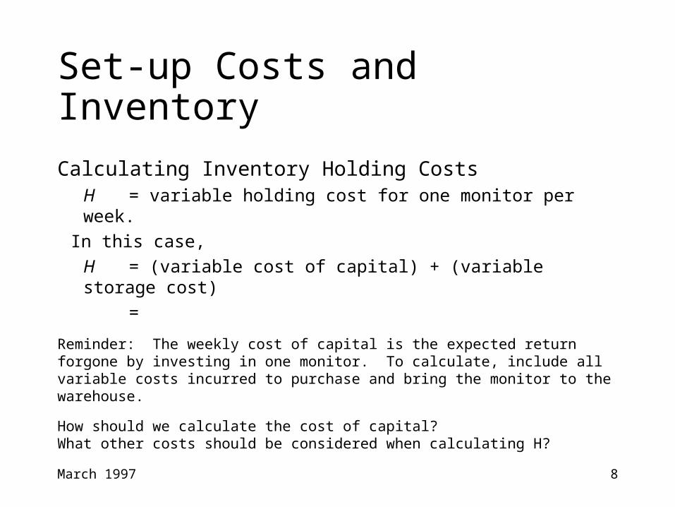
Set-up Costs and Inventory
Calculating Inventory Holding Costs H = variable holding cost for one monitor per week.
In this case,
H = (variable cost of capital) + (variable storage cost)
=
Reminder: The weekly cost of capital is the expected return forgone by investing in one monitor. To calculate, include all variable costs incurred to purchase and bring the monitor to the warehouse.
How should we calculate the cost of capital? What other costs should be considered when calculating H?

March 1997 9
The ‘Economic Order Quantity’ (EOQ)
Assume: – Constant, deterministic demand (D units/week)
– Known fixed cost per order placed ($S)
– Fixed unit price ($C/unit), independent of order size
– Holding cost associated with each unit of stock on hand ($H/unit/week)
– Fixed order quantity: Q units
– Instantaneous receipt of the ordered quantity

March 1997 10
Set-up Costs and Inventory
Holding and ordering costs for order size Qaverage inventory:
holding cost per week:
# of orders per week needed to fill demand D:
ordering cost per week:
March 1997 11
0
1000
2000
3000
4000
5000
6000
0 5000 10000 15000 20000
Order Quantity Q (monitors)
Ord
eri
ng
+ H
old
ing
Co
st
($/w
k)
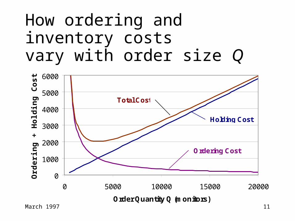
Ordering Cost
Total Cost
Holding Cost
How ordering and inventory costs vary with order size Q

March 1997 12
monitors 474,32
H
SDQ*EOQ
per week $2,015 =
2
Costs OrderingHolding
SDH
# Orders per week =
Costs Minimized by Q* = ‘EOQ’
This formula can be derived by plugging Q* into the cost formula

13
EOQ in Practice
• In practice, demand is not constant, so we’ll have trouble if we order the same amount each week
• Need to continually adjust the ordering pattern to actual demand:– Keep order frequency constant and vary order quantity
(e.g., ‘periodic’ or ‘base stock’ system)
– Keep order quantity constant and vary order frequency (e.g., ‘order point / order quantity’ or ‘Kanban’ system)
• In practice, order quantity or frequency will be rounded to some convenient value

14
0
20
40
60
80
100
120
0 1 2 3 4 5
Time
Inve
nto
ry O
n H
an
d +
On
Ord
er
Base stock system
Order periodically to bring inventory on hand + on order back to the base stock level; period length matches EOQ order frequency
Base stock level and period length together determine stockouts

15
Order point / order quantity (OP/OQ) system
Order the EOQ when inventory on hand + on order drops to the order point
0
20
40
60
80
100
120
0 1 2 3 4 5
Time
Inve
nto
ry O
n H
an
d +
On
Ord
er
Order point and order quantity together determine stockouts
March 1997 16
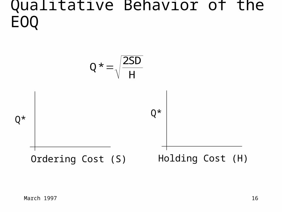
Qualitative Behavior of the EOQ
Ordering Cost (S)
Q*
Holding Cost (H)
Q*
Q*2SD
H
March 1997 17
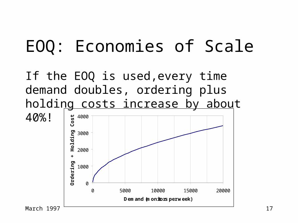
EOQ: Economies of Scale
0
1000
2000
3000
4000
0 5000 10000 15000 20000
Demand (monitors per week)
Ord
eri
ng
+ H
old
ing
Co
st
($/w
k)
If the EOQ is used,every time demand doubles, ordering plus holding costs increase by about 40%!
March 1997 18see: Principles of Corporate Finance, Brearly and Myers, pp. 774-779
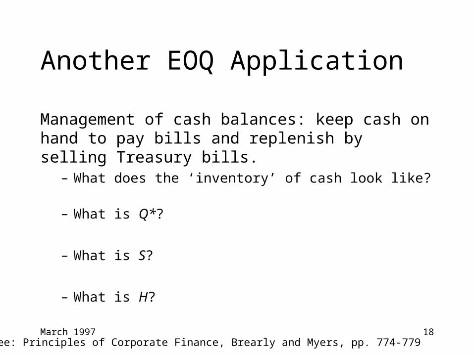
Another EOQ Application
Management of cash balances: keep cash on hand to pay bills and replenish by selling Treasury bills.
– What does the ‘inventory’ of cash look like?
– What is Q*?
– What is S?
– What is H?

March 1997 19
EOQ Generalizations
• Quantity discounts and price breaks
• Multiple products
• Discounting cash flows
• Variability in demand
• Finite production rate (EOQ assumes that the goods arrive all at once)
March 1997 20
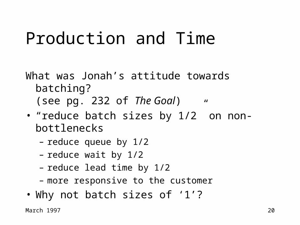
Production and Time
What was Jonah’s attitude towards batching? (see pg. 232 of The Goal)
• “reduce batch sizes by 1/2” on non-bottlenecks– reduce queue by 1/2
– reduce wait by 1/2
– reduce lead time by 1/2
– more responsive to the customer
• Why not batch sizes of ‘1’?

March 1997 21
What production plan should be used to meet demand for 1000 cars of each type per week? Demand for 600 cars of each type? For 100?
Flexible Production
• two types of cars: moon roof ()) and standard (*)• time to produce a batch is proportional to batch size
large batchproduction
plan
500 cars
)
setup
1 week
150
)
setup
150
*
setup
500 cars
*setup
500 cars
)
setup
500 cars
*
setup
150
)setup
150
*
setup
150
)
setup
150
*
setup
150
)
setup
150
*
setup
small batchproduction
plan
March 1997 22
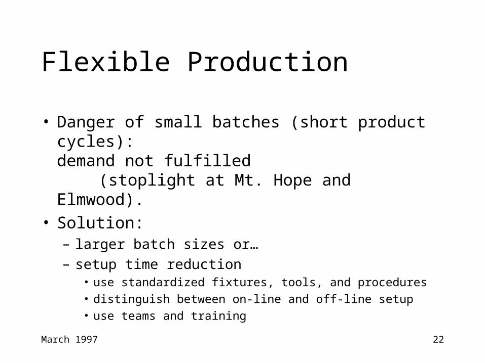
Flexible Production
• Danger of small batches (short product cycles): demand not fulfilled
(stoplight at Mt. Hope and Elmwood).• Solution:
– larger batch sizes or…
– setup time reduction• use standardized fixtures, tools, and procedures
• distinguish between on-line and off-line setup
• use teams and training
March 1997 23
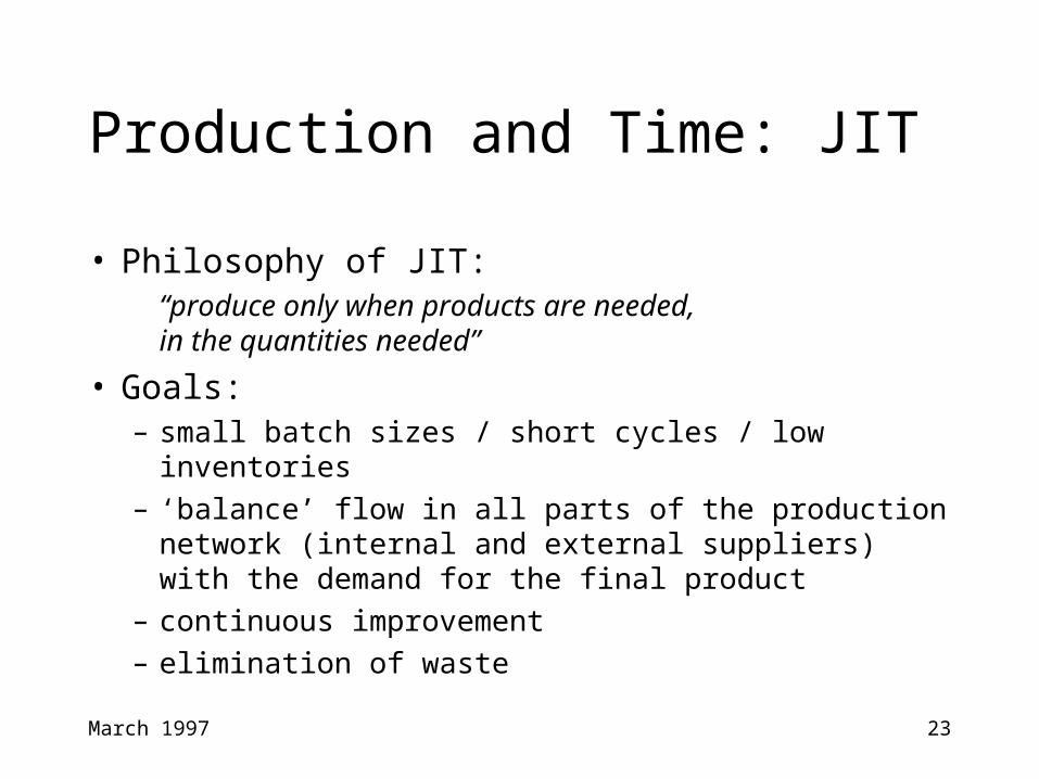
Production and Time: JIT
• Philosophy of JIT: “produce only when products are needed,
in the quantities needed”
• Goals:– small batch sizes / short cycles / low inventories– ‘balance’ flow in all parts of the production network
(internal and external suppliers) with the demand for the final product
– continuous improvement – elimination of waste

March 1997 24
JIT: Level Production (Heijunka)
• production with almost instantaneous setups
• models mixed and proportional to demand.
• Example: two standard cars sold for every one moon roof sold.Therefore, produce only two standard, one moon:
**)**)**)**)**)**)**)

March 1997 25
JIT: Level Production (Heijunka)
• also called ‘balanced’ or ‘mixed-model’ production• quick setups• small inventories• balanced flow throughout production process• But how short do setups have to be?
A mathematical model will tell us

March 1997 26
Summary of Insights
Inventory Models:– tradeoff between ordering and inventory costs
– economies of scale
Flexible Production:– long set-up times necessitate large batches; short set-
ups allow flexibility
– flexibility both requires, and encourages, the elimination of ‘waste’
Seek to “change the rules”: don’t take costs as given!