OM- Work Measurment Learning Curves

7/22/2019 OM- Work Measurment Learning Curves

http://slidepdf.com/reader/full/om-work-measurment-learning-curves 1/20

im, it takes 2,000 hours to build each electrical

generating turbine, so if we have to build ten, it

takes 20,000 hours. We should plan our budget

and price per generator based on 20,000 hours,”

exclaimed Pete Jacobs, the vice president of finance.

“No, Pete. According to my calculations, it will take

only 14,232 hours to build ten turbines and our total cost and

budget will be much lower than you think,” said Jim Conner,

the vice president of operations. “How do you get such crazy

numbers?” replied Jacobs.

WORK

MEASUREMENT,LEARNING CURVES,

AND STANDARDS

Operations Management

Part 4 Supplementary Chapter A

j

OM 2

© S t e f a n E d u a r d / P l a i n p i c t u r e / J u p i t e r I m a g e s

learningoutcomes

After studying this chapter you

should be able to:

L01 Explain the purpose of work

measurement.

L02 Describe how to apply time study

methods.

L03 Explain the principles and calculation

methods of work sampling.

L04 Explain the concept of a learning

curve and their application for

estimating production times.

What do you think?

Have you had an experience in

which the time it took to perform

some activity (such as solving a

Sudoku puzzle or playing an X-box

game) improved as your learning

increased?

A2 P a r t 4 : O M 2 S u p p l e m e n t a r y C h a p t e r s

62564_09_cA.indd 2 8/26/0



A3O M 2 S u p p l e m e n t a r y C h a p t e r A : W o r k M e a s u r e m e n t , L e a r n i n g C u r v e s , a n d S t a n d a r d s

Time standards represent reasonable estimates of the

amount of time needed to perform a task based on

an analysis of the work by a trained industrial engi-

neer or other operations expert. Jacobs cannot under-

stand the discrepancy between his estimate of 20,000

hours and Conner’s value of 14,232 hours to produce

a batch of turbines. The assembly of electrical power-generating turbines is a complex job with labor costs

for engineers and production employees approaching

$100 per hour. Obviously, a difference of 5,768 hours

can be significant in terms of cost, budgets, and pricing

decisions. Where did Conner get his figure? Moreover,

why should the total time to produce ten turbines

be less than 10 times the time to produce the first?

Many work tasks show increased performance over

time because of learning and improvement. Failure

to recognize this can lead to poor budgeting, errone-

ous promises for delivery, and other bad management

decisions.

In this supplementary chapter we introduce work

measurement, standards, and learning curves, and how

they are used in business. Most large corporations

develop standard times for routine work tasks using

work measurement. They are used in setting job perfor-mance standards, establishing recognition and reward

programs, and for compensation incentives. Valid stan-

dard times are vital to accomplishing most of the pro-

cess design and operations analysis methods described

in this text. Smaller businesses, especially service busi-

nesses, usually do not have such standard times for

their work activities and tasks. However, if one seeks to

improve operations, analyzing work and determining

standard times for key work activities and processes is

a crucial first step.

A

© M a s o n M o r fi t / G e t t y I m a g e s

62564_09_cA.indd 3 8/26/0




operating conditions. The prescribed method to perform

a task is usually developed by industrial engineers who

identify the most efficient and safest procedure.

However, not everyone works at the same pace,

and people may either slow down or speed up their

effort when they are being observed. Thus, observed

times must be adjusted by a factor that accounts for theworker’s effort. Normal times are calculated using the

following equation:

Normal time 5

Observed time 3 Performance rating factor 5

OT 3 PRF [A.1]

The performance rating factor (PRF) is a judgment

made by the person doing the time study as to whether

the employee is working at the normal pace (that is,

1.0 or 100 percent), below the normal pace (that is,

less than 1.0 or 100 percent), or above the normal pace

(that is, greater than 1.0 or 100 percent). For exam-

ple, a PRF of 115 percent indicates that work is being

performed at a pace that is 15 percent above normal.

Typically, three or more highly trained work study ana-

lysts make these judgments independently and then the

average PRF is used in equation A.1. For example, if

work study analyst A rates an employee at PRF 5 1.2

and an observed time of 2.5 minutes per unit, B rates

the same employee at PRF 5 1.0 and an observed time

of 2.2 minutes per unit, and C rates the same employee

at PRF 5 0.9 and an observed time of 2.1 minutes per

unit, then, using equation A.1, the normal time is 2.363

minutes per unit (1.2 3 2.5 1 1.0 3 2.2 1 0.9 3 2.1)/3.

Normal times must also be adjusted for personaltime and unavoidable delays. Allowances include time

for labor fatigue and personal needs, equipment break-

downs, rest periods, information delays, and so on.

Most allowance factors are in the range of 10 to 20 per-

cent. Standard time is normal time adjusted for allow-

ances. It is computed using the following equation:

Standard time 5

Normal time (1 1 Allowance factor) [A.2]

For example, if the normal time is 2.363 and an allow-

ance factor of 1.2 is used, the standard time is 2.836

minutes per unit.The performance rating factor and allowance fac-

tor are based on human judgments, and therefore, the

procedure for establishing standard times must include

audits, third-party reviews, and extensive training and

retraining of work-study analysts to keep them prop-

erly calibrated. Videotapes of employee work activities

are often used to train work-study analysts.

1 Work Measurement perations managers are inter-

ested in how long it takes to

create an output or outcome, or

equivalently, how much can be

produced over a certain length

of time. Work measurement is

a systematic procedure for the

analysis of work and determination of times required

to perform key tasks in processes.Work measurement

leads to the development of labor and equipment time

standards that are used for

• estimating work-force and equipment capacity,

• establishing budgets,

• determining what new work procedures will cost,

• evaluating time and cost trade-offs among process

design alternatives,

• establishing wage-incentive systems,

• monitoring and evaluating employee performance

and productivity, and

• providing accurate information for scheduling and

sequencing.

Without accurate time standards it is impossible to per-

form these tasks. For example, the process of assembly-

line balancing, discussed in Chapter 8, requires accurate

estimates of the standard time required to perform each

task or work activity.

Standard times are management’s anchor in an uncer-

tain operating environment. To establish usable standards,work tasks and activities must be carefully defined and

studied. Thus, job and pro-

cess analysis should precede

work measurement. How

long it takes to perform a

task depends on the work-

er’s pace, operating condi-

tions, and work method.

Normal time is the expected

time required to perform

some work activity at a

normal pace, under normal

operating conditions, andusing a prescribed method.

By a normal pace, we mean

a pace that can be consis-

tently performed by the

average employee without

undue fatigue under normal

Work measurementis a systematic procedure

for the analysis of work and

determination of times

required to perform key tasks

in processes.

Normal time is the ex-

pected time required to per-

form some work activity at a

normal pace, under normal

operating conditions, and

using a prescribed method.Allowances include time

for labor fatigue and personal

needs, equipment break-

downs, rest periods, informa-

tion delays, and so on.

Standard time is normal

time adjusted for allowances.

o

62564_09_cA.indd 4 8/26/0




Work Measurement Activities in RollerCoaster Maintenance

A popular roller coaster called the Runaway Mine Train

(RMT) requires extensive inspections, maintenance,

and repair to keep it running and earning revenue. Dur-

ing peak season, the RMT is expected to operate 16hours per day. Each part of the RMT, from structural

steel uprights to the bearings in the wheels, must be

inspected and well maintained. All RMT daily work

tasks are grouped into work activities such as complete

train inspection, track inspection, electrical inspection,

cleaning the trains, and vehicle inspection. Each work

activity is assigned a craft employee such as a track

and vehicle machinist, electrician, sound engineer, cus-

todian, oiler, software and computer operator, and so

on. Sixty-one distinct jobs existed for this attraction but

only the jobs related to inspection, maintenance, and

repair were to be time studied.

A sampling plan was established and the data col-

lected. Once time standards were determined for all

maintenance-related tasks, the number of employees

required was computed. Preventive maintenance wasdone each Wednesday and required additional change-

over or setup time. Two teams were established, each

with four people. One team worked Sunday to Wednes-

day and the second team from Wednesday to Saturday.

The two teams overlapped on Wednesday for one-half

day to get all preventive maintenance done. Work mea-

surement information and analysis plays a major role in

achieving the objectives of operating safety, efficiency,

and profitability.1

Solved Problem

Assume your first job out of school is as a branch

manager for a major bank. Your branch also has a

back-office operation where bank packs of $300 are

assembled for retail businesses. Each bank pack con-

tains two $20 bills, ten $10 bills, twelve $5 bills, and

one hundred $1 bills. Retail customers become upset

when these bank packs are not available since they

usually pick them up before their retail store opens.A continuous stopwatch study collected the informa-

tion shown in the table below. The policy of the bank

is to use a 20 percent allowance factor for branch bank

operations. (a) What is the normal and standard time

for a bank pack? (b) How long would it take to pack

200 packs? Now you must decide how many branch

bank staff to assign to this work activity and when they

will do the work.

Solution:

a. To determine the normal and standard times, notethat the continuous stopwatch study timed eachdenomination separately and the cumulative timesare shown across each row. The “Difference” rowsshow the individual times.

b. (200 bank packs)(31.426 minutes)/10 bank packs 5 (20)(31.426 minutes) 5 628.5 minutes or 10.5 hours

Observation Cycles (cumulative, in minutes) Performance NormalWork Task 1 2 3 4 5 6 7 8 9 Average Rating Time

Count 2 $20s 0.11 0.15 0.36 0.50 0.65 0.78 0.89 1.02 1.22

Difference 0.11 0.21 0.14 0.15 0.13 0.11 0.13 0.20 0.15 1.15 0.170

Count 10 $10s 0.25 0.66 0.94 1.27 1.79 2.05 2.36 2.77 3.20

Difference 0.25 0.28 0.33 0.52 0.26 0.31 0.41 0.43 0.35 0.95 0.331

Count 12 $5s 0.37 0.79 0.93 1.44 1.91 2.30 2.88 3.61 4.22

Difference 0.37 0.14 0.51 0.47 0.39 0.58 0.73 0.61 0.48 1.00 0.475Count 100 $1s 1.02 2.44 3.70 5.01 6.39 8.11 9.43 10.55 11.55

Difference 1.02 1.26 1.31 1.38 1.72 1.32 1.12 1.00 1.27 1.10 1.393

Place Bank Packs in Tray (once every ten cycles) 5 2.50 1.00

Standard time per bank pack 5 Normal time 3 (1 1 Allowances) 5 2.8426

Standard time per ten bank packs with setup 5 31.426

Normal processing (run) time per bank pack 5 2.369

Normal time per ten bank packs with setup 5 26.188

62564_09_cA.indd 5 8/26/0




2 Time Study Methodsime study is the development of a

standard time by observing a task

and analyzing it with the use of a

stopwatch (see the feature below:

Job Description—City of Phoenix,

Arizona). The general approach to

time study can be described

as follows.

1. Define and evaluate each

task and activity. Thisincludes determiningwhat level of detail isbest for time study

measurements, and then grouping or separating tasksaccordingly.

2. Measure and record the time needed to perform each

task or activity over a number of cycles. A trainedobserver with a stopwatch usually does this. Anumber of observations should be taken to account

for variability in performance. Assuming that thedistribution of task times is normally distributedfor each task, the number of cycles that should beobserved is determined statistically by the sample size(n) formula, equation A.3:

n $ (za /2

)2σ

2 / E2 [A.3]

where za /2

is the value of the standard normal distri-

bution having an area of α /2 in the upper tail, σ isan estimate of the standard deviation, and E is the

t Job Description—City of Phoenix, ArizonaThe city of Phoenix, Arizona posted this job descrip-

tion for an “operations analyst.” The job is to design,

conduct, and participate in major work standards and

systems analyses covering a wide variety of government

functions. Considerable flexibility is allowed in this job

for designing and conducting each study. Assignments

are comprehensive and entail interactions between

major government and civic organizational units. The

duties also involve substantial contact with high-level

government officials, so writing and presentation skills

are essential.

Operations Analyst for City of Phoenix, Arizona

Essential Job Requirements:

• Designs systems, procedures, forms, and work

measurements to effect methods improvement, worksimplification, improvement of manual processing, orfor adaption to computer processing;

• Designs control reporting systems for use in unit

measurement for evaluation of performance and fordetermination of staffing levels and recommendsstaffing levels to section chief;

• Studies operational problems such as ofce space

utilization, equipment utilization, managementreporting systems, staffing patterns, process efficiency,and prepares written recommendations for changesand/or improvements;

• Develops project plans to achieve established objec-tives and time schedules;

• Writes and/or edits manuals for uniform use of new

or revised procedures and policies;

• Evaluates ofce machines and ofce or heavy opera-tions equipment relative to quality, price, and deter-mination of best equipment;

• Organizes, authors, and presents oral and written

research reports;

• Identies work elements in detail and develops

complex flow charts, work standards, and workmethod improvements;

• Demonstrates continuous effort to improve opera-tions, decrease turnaround times, streamline workprocesses, and work cooperatively and jointly toprovide quality seamless customer service.

Required Knowledge, Skills and Abilities:

• Principles of work measurement and activity analysis.

• Principles of statistical methods and techniques.

• Employ work measurement techniques, i.e., stop-watch, pre-determined data, and time ladders.

• Understand and carry out oral and written instruc-tion provided in the English language.

• Conduct studies and research with minimal supervision.

• Complete assignments with independent thought and

action within the scope of specific assignments.

• Work cooperatively with other City employees,

outside regulatory agencies, and the public.

• Enter data or information into a terminal, PC, or otherkeyboard device using various software packages.

• Communicate orally with customers, co-workers,

and the public in face-to-face one-on-one settings, ingroup settings, or using a telephone.

• Produce written documents with clearly organized

thoughts using proper English sentence construction,punctuation, and grammar.2

Time study is the develop-

ment of a standard time

by observing a task and

analyzing it with the use of a

stopwatch.

62564_09_cA.indd 6 8/26/0




desired sampling error. When timing a work activitywith multiple tasks, the general rule is to take thelargest sample size estimate from equation A.3 forall tasks.

3. Rate the employee’s performance of each task or

activity. As noted, rating human performance accu-

rately requires considerable training.4. Use the performance rating and equation A.1 to

determine the normal task time. The sum of thosetask times is the normal time for the entire workactivity.

5. Determine the allowance factor for the work activity.

6. Determine the standard time using equation A.2 .

To illustrate time stud-

ies, we will consider a simple

manual assembly process.

Exhibits A.1 and A.2 show

a faucet stem assembly and

an operations activity chart,

which provide the basis for developing the time study. Anoperations activity chart is a detailed analysis of work

motions performed for a manual task.

Because these “micromotions” are typically so

small that it would be difficult to measure them eas-

ily, we usually combine several smaller work tasks into

larger activities. For instance, the tasks “get washer”

An operations activitychart is a detailed analysis

of work motions performed

for a manual task.

Exhibit A.1 Faucet Stem Assembly

StemHousing Washer Screw

Exhibit A.2 Operations Activity Chart of Faucet Stem Assembly

Get Housing

Left hand Right hand

Get stem

Screw in stem

Get washer

Insert washer

Get screw

Insert screw

Get screwdriver

Tighten screw

Release screwdriver

Operation chart

Present method

Faucet stem assembly

Hold Housing

Place assembly in tray

62564_09_cA.indd 7 8/26/0




A spreadsheet that can be used for a typical time

study when continuous timing is used is shown in

Exhibit A.3. Continuous timing involves starting the

clock at the beginning of each task and recording the

cumulative time at the completion of each work task.

The task times are found by subtracting successive

cumulative times. These are added and averaged toobtain the mean time for each work task. Performance

ratings are given in the next-to-last column. By mul-

tiplying the performance-rating factor by the average

observed time, we obtain the normal time for each work

task and add them. Next the allowances are determined

to compute the standard time. For the faucet-stem

assembly, we assume a 5 percent personal allowance,

5 percent fatigue allowance, and 10 percent delay of

materials allowance. Therefore, the total allowance fac-

tor is 20 percent.

The standard time for the faucet stem assembly job

is then computed, using equation A.2, as: Standard time

5 (0.550)(1 1 .2) 5 0.660 minutes per faucet assem-

bly. Thus, an assembler of faucet-stem assemblies can

be expected to produce at a standard rate of 1/0.660

parts per minute, or about 91 parts per hour. In a

and “insert washer” might be combined. This leads to

the following set of work activities:

1. Get housing and stem.

2. Screw in stem.

3. Get and insert washer.

4. Get and insert screw.5. Tighten screw.

6. Place completed assembly in tray.

To determine the sample size needed for a time study,

suppose we desire a 90 percent probability that the

value of the sample mean provides a sampling error

of .01 minute or less. Further assume that σ is esti-

mated from historical experience to be .019. Therefore,

α5 .10, z.05

5 1.645, and E 5.01. Using equation A.3,

we compute

n 5 (1.645)2(.019)2 /(.01)2 5 9.8 10 observations

A sample size of 10 or more will provide therequired precision. (Fractional values of n should

always be rounded upward to ensure that the precision

is at least as good as desired.)

Exhibit A.3 A Spreadsheet for Time Study (This spreadsheet is available on the Premium Website.)

62564_09_cA.indd 8 8/26/0




7-hour workday with 1 hour off for lunch and breaks,

an assembler can produce (7)(91) 5 637 faucet-stem

assemblies per workday.

2.1 Using Regression

Analysis to DetermineStandard TimeRegression analysis provides an alternative method to

estimating the time required to do a particular job or

work activity. Regression analysis is used to predict

times based on different attributes of the work, rather

than by adding up individual task times. Using regres-

sion to estimate standard times can be advantageous

because it avoids the assumption of additive task times

when this might not hold; statistically significant vari-

ables can be determined; confidence intervals for the

prediction can be developed; and finally, it may cost lessthan a detailed work study.

Consider the following problem on developing

standard time estimates for installing electrical power

lines. An electric power company wishes to determine a

standard time-estimating formula for installing power

lines. A good formula would help it plan capacity and

staffing needs. The following data are collected:

Total Wire No. of No. ofTime Number (100 Cross No. of Guy

(hours) of Poles feet) Arms Insulators wires

8.0 1 4 1 2 114.0 2 10 2 4 0

17.5 3 6 3 6 1

7.0 1 2.5 2 3 0

16.0 2 10 4 6 0

37.5 4 24 8 12 2

39.5 4 33 7 11 1

10.5 1 3 2 4 2

17.0 2 8 4 8 1

23.5 3 12 6 12 0

16.5 2 12 2 4 1

22.0 3 18 3 6 0

8.5 1 5 2 3 0

28.5 4 12 8 12 0

Exhibit A.4 shows the results using Excel’s Regres-

sion tool. The model obtained from this analysis is

Time 5 0.237 1 2.804 Poles 1 0.514 Wire 1 1.09

Cross arms 1 0.170 Insulators 1 1.50 Guy

wires

Exhibit A.4 Results of Regression Analysis for Electric Power Line Installation

62564_09_cA.indd 9 8/26/0




2.3 The Debate Over WorkStandardsWork standards evolved at the turn of the twentieth

century, and although they have supported significant

gains in productivity, they have been the subjects ofdebate since the quality revolution began in the United

States. Critics such as W. Edwards Deming have con-

demned work standards on the basis that they destroy

intrinsic motivation in jobs and rob workers of the cre-

ativity necessary for continuous improvement. That is

certainly true when managers dictate standards in an

effort to meet numerical goals set up by their superiors.

However, the real culprit in that case is not the stan-

dards themselves, but managerial style. The old style of

managing reflects Taylor’s philosophy: Managers and

engineers think, and workers do what they are told. A

total quality approach suggests that empowered work-

ers can manage their own processes with help frommanagers and professional staff.

Experience at GM’s NUMMI plant has shown that

work standards can have very positive results when

they are not imposed by dictum, but designed by the

workers themselves in a continuous effort to improve

productivity, quality, and skills.3 At the GM-Fremont

plant, industrial engineers performed all of the meth-

ods analysis and work-measurement activities, design-

ing jobs as they saw fit. When the industrial engineers

were performing motion studies, workers would natu-

rally slow down and make the work look harder. At

NUMMI, team members learned techniques of workanalysis and improvement, then timed one another

with stop-watches, looking for the safest, most efficient

way to do each task at a sustainable pace. They picked

the best performance, broke it down to its fundamen-

tal elements, and then explored ways to improve the

task. The team compared the analyses with those from

other shifts at the same workstation, and wrote detailed

specifications that became the work standards. Results

were excellent. From a total quality perspective, this

was simply an approach to reduce variability. In addi-

tion, safety and quality improved, job rotation became

more effective, and flexibility increased.

The regression analysis shows a high R2 value,

showing a strong fit to the data. Moreover, the p val-

ues for the regression coefficients are significant, mean-

ing that each of the variables contributes to predicting

time. If the utility faces a situation in which it estimates

installation of 4 poles, 1,500 feet of wire, 7 cross arms,

12 insulators, and no guy wires, the predicted time forthe job would be

Time 5 0.237 1 2.804 3 4 1 0.514 3 1500 1 1.09

3 7 1 0.170 3 12 1 1.50 3 0 5 792 hours

2.2 Predetermined TimeStandard MethodsPredetermined time standards describe the amount

of time necessary to accomplish specific movements

(called micromotions), such as moving a human hand a

certain distance or lifting a 1-pound part. These small

time estimates have been documented and are available

in books and electronic tables. If a job, work activity,

or task can be broken down into such elemental tasks,

an estimate of the normal time is made by adding up

these predetermined times. This approach is especially

appealing for developing standard times for new manu-

factured goods and some service tasks. An electronics

manufacturer, for example, may have much experience

with assembling small electronic components using

human labor and keep a record of past micromotion

and normal time analyses. For similar new tasks and

electronic component parts, predetermined time stan-dards can be used to estimate new normal times. Pre-

determined time standards were originally developed

for labor-intensive human tasks but data sets exist for

machine micromovements, such as those involving an

automated drill press.

Predetermined time standards are advantageous

since they cost less than a stopwatch time study, avoid

needing multiple performance ratings, and are best for

new goods and services. However, this type of micro-

motion-based time standard is not justified for small

order sizes or infrequent production runs. In addition,

once the new good or service and its associated pro-

cess are stable and running well, stop-watch or work-

sampling time studies still need to be done. Finally, the

assumption of additivity is sometimes questionable,

since a process or assembly sequence of difficult versus

simple micromotions may or may not be additive.

62564_09_cA.indd 10 8/26/0




Suppose that a new voice-

activated word process-

ing software could greatly

increase productivity

in typing, spell check-

ing, and revising techni-

cal papers. However, thepurchase of this product

is not justified unless it is

used a significant percentage of the time. To determine

the percentage of time secretaries spend performing the

relevant work activities, we could observe them at ran-

dom times and record their activities. If 100 observa-

tions are taken, we might get the results in Exhibit A.5.

The percentage of time spent typing or revising

is 21 percent 1 7 percent 5 28 percent. To determine

the needed sample size (that is, the number of obser-

vations), suppose we want to estimate the proportion

of time spent typing to 65 percent, with a 95 percent

probability. We use equation A.4, with E 5 0.05 and

zα /2

5 1.96. Suppose the head secretary estimates that

40 percent of the time is spent typing. This provides a

value for p of 0.4. Then the needed sample size using

equation A.4 is

n $ (1.96)20.4(1 2 0.4)/0.052 5 368.8 or at least

369 observations

If that is to be done over a 1-week (40-hour) period,

it represents approximately 9 observations per hour

(9.225, to be exact). The observations should be taken

randomly when work is at a normal level (not during

the spring break!).

3 Work Samplingork sampling is a

method of randomly

observing work over

a period of time to

obtain a distribu-

tion of the activities

that an individual or

a group of employees perform. Work sampling

determines the proportion of time spent doing cer-

tain activities on a job. It can be used to determine

the percentage of idle time and also as a means

of assessing nonproductive time to determine per-

formance ratings or to establish allowances. Work

sampling is based on the binomial probability dis-

tribution, because it is concerned with the propor-

tion of time that a certain activity occurs. Thus,

the sample size (n) for a work-sampling study isfound by using equation A.4:

n $ (zα /2

)2 p(1 2 p)/ E2 [A.4]

where p is an estimate of the population proportion

of the binomial distribution. Obviously, p will never

be known exactly, since it is the population parameter

we are trying to estimate. We can choose a value for p

from past data, a preliminary sample, or a subjective

estimate. If p is difficult to determine in those ways, we

can select p 5 0.5, since it gives us the largest value for

p(1 2 p) and therefore provides the largest and most

conservative sample size.To illustrate work sampling, consider the secre-

tarial staff in a college department office. The secretar-

ies spend their time in various ways, such as

• answering the telephone

• typing drafts of technical papers

• revising technical papers

• talking to students

• duplicating class handouts

• other productive activities

• personal time

• idle periods

Work sampling is a meth-

od of randomly observing

work over a period of time to

obtain a distribution of the

activities that an individual

or a group of employees

perform.

w

Exhibit A.5 Work Sampling ActivityFrequency Data

Activity Frequency

Answering the telephone 14

Typing drafts 21

Revising papers 7

Talking to students 10

Duplicating 15Other productive activity 25

Personal 6

Idle 2

TOTAL 100

62564_09_cA.indd 11 8/26/0




4 Learning Curveshe learning curve concept is thatdirect labor unit cost decreases in

a predictable manner as the experi-

ence in producing the unit increases.

For most people, for example, the

longer they play a musical instru-

ment or a video game, the better

and faster they become. The same is true in assem-

bly operations, which was recognized in the 1920s at

Wright-Patterson Air Force Base in the assembly of air-

craft. Studies showed that the number of labor hours

required to produce the fourth plane was about 80 per-

cent of the amount of time spent on the second; theeighth plane took only 80 percent as much time as the

fourth; the sixteenth plane 80 percent of the time of the

eighth, and so on. The decrease in production time as

the number produced increases is illustrated in Exhibit

A.6. As production doubles from x units to 2x units, the

time per unit of the 2xth unit is 80 percent of the time

of the xth unit. This is called an 80 percent learning

curve. Such a curve exhibits a steep initial decline and

then levels off as employees become more proficient in

their tasks. In general, a p-percent learning curve char-

acterizes a process in which the time of the 2xth unit is

p percent of the time of the xth unit.

Defense industries (for example, the aircraft andelectronics industries), which introduce many new

and complex products, use learning curves to estimate

labor requirements and capacity, determine costs and

To take a random sample, we can use the table

of random digits in Appendix C. There are several

ways to use random digits in deciding when to take

observations. For this example, an average of 9.225

observations per hour requires the observations to

be spaced, on the average (60/9.225) 5 6.5 minutes

apart. We should not take observations exactly 6.5minutes apart, however, for then the sample would

not be random. Suppose observations are between 3

and 10 minutes apart. If they are random, the aver-

age is 6.5 minutes. We can use the random digits

as follows. Suppose the first observation is taken

at 9:00. We choose numbers from the first row of

Appendix C to find how many minutes later we

should take the next observation (0 represents 10

minutes, and we discard any 1s or 2s). For instance,

the first number is 6; thus we take the next obser-

vation at 9:06. The next number is 3, so the third

observation is made at 9:09. We discard the 2 and

take the next observation 7 minutes later, at 9:16.

We see that the time and cost required to take a ran-

dom sample can be significant; that is one of the

disadvantages of random sampling.

Work sampling is based on statistics, and like all

statistical procedures, it

can suffer from sampling

error and lead to erro-

neous conclusions sim-

ply by chance. Also, as

the famous Hawthorne

experiments showed,

people often changetheir behavior when

being observed, and this

t

The learning curveconcept is that direct

labor unit cost decreases in

a predictable manner as the

experience in producing the

unit increases.

A p-percent learningcurve characterizes a pro-

cess in which the time of the

2 x th unit is p percent of the

time of the x th unit.

Solved Problem

In a work-sampling study an administrative assistant

was found to be working 2,700 times in a total of 3,000

observations made over a time span of 240 working

hours. The employee’s output was 1,800 forms. If a per-

formance rating of 1.05 and an allowance of 15 percentare given, what is the standard output for this task?

Solution:

Effective number of hours worked 5 2,700(240)/3,000

5 216.

Output during this period 5 1,800 forms.

Actual time per form 5 216(60)/1,800 5 7.2 minutes,

or 8.33 forms per hour.

Normal time 5 Actual observed time 3 Performance

rating 5 7.2(1.05) 5 7.56 minutes.Standard time 5 7.56(1.15) 5 8.694 minutes per form.

Standard output 5 60/8.694 5 6.9 forms per hour, or

55 forms per 8-hour day.

can influence the results. Thus, work sampling should

be used with caution.

62564_09_cA.indd 12 8/26/0




budget requirements, and plan and schedule production.

Eighty-percent learning curves are generally accepted as

a standard, although the ratio of machine work to man-

ual assembly affects the curve percentage. Obviously, no

learning takes place if all assembly is done by machine.

As a rule of thumb, if the ratio of manual to machine

work is 3 to 1 (three-fourths manual), then 80 percent

is a good value; if the ratio is 1 to 3, then 90 percent is

often used. An even split of manual and machine work

would suggest the use of an 85 percent learning curve.

The learning factor may also be estimated from past

histories of similar parts or products.

Mathematically, the learning curve is represented

by the function

y 5 ax2b [A.5]

where

x 5 number of units produced,

a 5 hours required to produce the first unit,

y 5 time to produce the xth unit, and

b 5 constant equal to 2ln p /ln 2 for a 100 p percent

learning curve.

Thus, for an 80 percent learning curve, p 5 0.8 andb 5 2ln 0.8/ln 2 5 2(2 0.223)/0.693 5 0.322

For a 90 percent curve, p 5 0.9 and

b 5 2ln 0.9/ln 2 5 2(2 0.105)/0.693 5 0.152

Although the learning curve theory implies that

improvement will continue forever, in actual practice

the learning curve flattens out. As management inter-

est in the initial creation of a new good or service

decreases, employees may reach a level of production

that is expected of them and hold that rate. Another

way to view the theory of learning is that early on

extraordinary new practices and methods are found to

dramatically improve performance, such as substituting

plastic for steel parts. Later in the life of the learning

curve, the focus shifts to incremental improvements.

Learning curves can apply to individual employees

or, in an aggregate sense, to the big-picture initiatives

such as pricing strategy. For example, learning curves

are used to monitor employees typing and encoding

checks in a bank’s operations. Each employee must

reach a certain threshold-learning rate within 6 months

or more training is required. In some cases, the bank-

encoding employee is transferred to another bank job

because the employee is just not suited to the encoding

job. Learning curves help managers make such deci-

sions. From an aggregate and strategic perspective, a

firm may use the learning-curve concept to establish

a pricing schedule that does not initially cover cost in

order to gain increased market share.

Managers should realize that improvement alonga learning curve does not take place automatically.

Learning-curve theory is most applicable to new prod-

ucts or processes that have a high potential for improve-

ment and when the benefits will be realized only when

appropriate incentives and effective motivational

tools are used. Organizational changes may also have

Exhibit A.6 An 80 Percent Learning Curve

Number produced

100

80

60

40

20

5 10 15

T i m e p e r u n i t a s a p e r c e n t

a g e

o f f i r s t u n i t

62564_09_cA.indd 13 8/26/0




employees for 125, and 83 for 225. Clearly, under-

standing learning is important for aggregate planning.

Values for learning-curve functions can be easily

computed and summarized through the use of tables.

Exhibits A.8 and A.9 present unit values and cumula-

tive values, respectively, for learning curves from 60

percent through 95 percent. To find the time to producea specific unit, multiply the time for the first unit by the

appropriate factor in Exhibit A.8. For the 90 percent

learning-curve example presented earlier, the time for

the second unit is 3,500(0.9000) 5 3,150. The time for

the third unit is 3,500(0.8462) 5 2,961.7, and so on.

To find the time for a cumulative number of units,

we can use Exhibit A.9. Thus, for a 90 percent learn-

ing curve, if the time for the first unit is 3,500, the

time for the first 25 units is 3,500(17.7132) 5 61,996.

Similarly, the time for the first 100 units is

3,500(58.1410) 5 203,494. The values in Exhibit A.7

were found using this table.

A broader extension of the learning curve is the

experience curve. The experience curve states that the

cost of doing any repetitive task, work activity, or proj-

ect decreases as the accumulated experience of doing

the job increases. The terms improvement curve, expe-

rience curve, and manufacturing progress function are

often used to describe the learning phenomenon in the

aggregate context. Marketing research, software design,

developing engineering specifications for a water plant,

accounting and financial auditing of the same client,

implementing a software integration project, and so

on are examples of this broader view. The idea is that

each time experience doubles, costs decline by 10 per-cent to 30 percent. Costs must always be translated into

significant effects on learn-

ing. Changes in technol-

ogy or work methods will

affect the learning curve,

as will the institution of

productivity and quality-

improvement programs.As an illustration of learning curves, suppose a

manufacturing firm is introducing a new and complex

machine and has determined that a 90 percent learning

curve is applicable. Estimates of demand for the next 3

years are 50, 75, and 100 units. The time to produce the

first unit is estimated to be 3,500 hours. Therefore, the

learning-curve function is

y 5 3,500x20.152

Consequently, the time to manufacture the second unit

will be

3,500 (2)20.152

5 3,150 hoursExhibit A.7 gives the cumulative number of hours

required to produce the 3-year demand in increments of

25 units. Thus, to produce the 50 units in the first year,

the firm will require 112,497 hours. If we assume that

each employee works 160 hours per month, or 1,920

hours per year, we find that for the first year the firm

will need

112,497/1,920 5 59 employees

to produce this machine. In the second year, the total

number of hours required will be the difference between

the cumulative requirements for the first two years’production (246,160 hours) and the first year’s produc-

tion (112,497 hours), or

246,160 2 112,497 5 133,663 hours

So the labor requirements for the second year are

133,663/1,920 5 70 employees

Similarly, for the third year, the labor requirements are

406,112 2 246,160 __________________ 1,920

5 83 employees

These are aggregate numbers; at a more detailed plan-

ning level, they will vary according to how productionis actually scheduled over the year. Also, note that the

number of employees required to produce these units

increases in a nonlinear way, reflecting the learning

that is taking place among employees. For example,

we might need 59 employees to produce 50 units, 70

Exhibit A.7 Cumulative Time

Required Using Learning Curves

Cumulative Units Cumulative Hours Required

25 61,996

50 112,497

75 159,164

100 203,494

125 246,160150 287,545

175 327,894

200 367,374

225 406,112

The experience curve

states that the cost of doing

any repetitive task, work ac-

tivity, or project decreases as

the accumulated experience

of doing the job increases.

62564_09_cA.indd 14 8/26/0




4. Changes in product design, raw material usage, tech-nology, and/or the process may significantly alter thelearning curve.

5. Humans learn simple task(s) quickly and reach alimit on learning for the task(s), but for complexintellectual task(s) such as software programming,learning is less limited and may continue. The firsttype of learning is described with an exponentialcurve; the more complex learning is sometimesdescribed by an S-shaped curve.

6. A contract phaseout may result in a lengthening ofprocessing times for the last units produced, sinceemployees want to prolong their income period.

7. The lack of proper maintenance of tools and equip-ment, the nonreplacement of tools, or the aging ofequipment can have a negative impact on learning.

8. Keeping groups of employees together, such as highlyspecialized consulting groups, reaps a productivitybenefit but may stifle innovation and new experi-ences.

9. The transfer of employees may result in an interrup-tion or a regression to an earlier stage of the learningcurve or may necessitate a new learning curve.

10. Learning curves focus on direct labor and ignoreindirect labor that also contributes to efficiency andeffectiveness.

constant dollars to eliminate the inflation effect. Of

course, the learning or experience curve does not con-

tinue this dramatic decrease in time and costs indefi-

nitely, and at some point begins to flatten out.

4.1 Practical Issues in UsingLearning CurvesThe following ten factors can affect the applicability

of the learning or experience curve and/or the amount

of learning that occurs. Good management judgment

is required to recognize these factors and take appro-

priate action, including stopping the current learning-

curve analysis, beginning a new learning-curve analysis,

and/or using other planning methods for the remainder

of the work.1. The learning curve does not usually apply to super-

visory personnel, some skilled craftspeople, or jobsthat have nonrepetitive job tasks.

2. A change in the ratio of indirect labor or supervisorytalent to direct labor can alter the rate of learning.

3. The institution of incentive systems, bonus plans,quality initiatives, empowerment, and the like mayincrease learning.

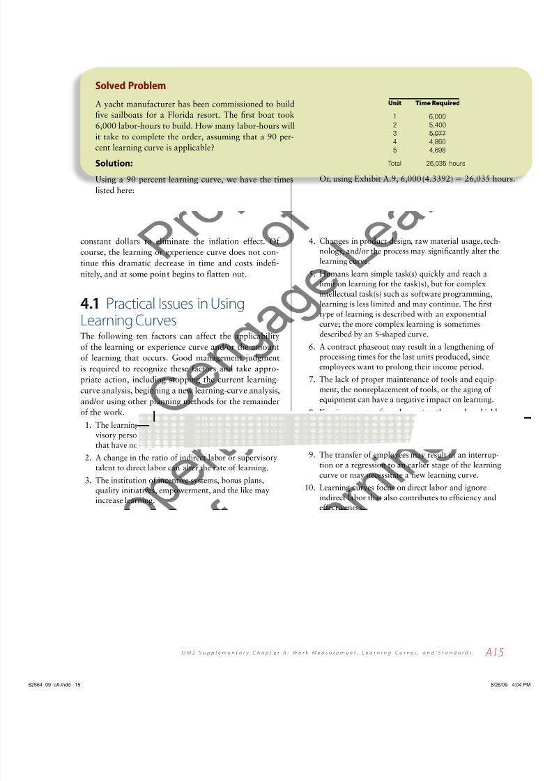
Solved Problem

A yacht manufacturer has been commissioned to build

five sailboats for a Florida resort. The first boat took

6,000 labor-hours to build. How many labor-hours will

it take to complete the order, assuming that a 90 per-cent learning curve is applicable?

Solution:

Using a 90 percent learning curve, we have the times

listed here:

Unit Time Required

1 6,000

2 5,400

3 5,077 4 4,860

5 4,698

Total 26,035 hours

Or, using Exhibit A.9, 6,000(4.3392) 5 26,035 hou

62564_09_cA.indd 15 8/26/0




Exhibit A.8 Unit Values for Learning Curves

p .60 .65 .70 .75 .80 .85 .90 .95

x b .737 .621 .515 .415 .322 .234 .152 .074

1 1.0000 1.0000 1.0000 1.0000 1.0000 1.0000 1.0000 1.0000

2 0.6000 0.6500 0.7000 0.7500 0.8000 0.8500 0.9000 0.9500

3 0.4450 0.5052 0.5682 0.6338 0.7021 0.7729 0.8462 0.9219

4 0.3600 0.4225 0.4900 0.5625 0.6400 0.7225 0.8100 0.9025

5 0.3054 0.3678 0.4368 0.5127 0.5956 0.6857 0.7830 0.8877

6 0.2670 0.3284 0.3977 0.4754 0.5617 0.6570 0.7616 0.8758

7 0.2383 0.2984 0.3674 0.4459 0.5345 0.6337 0.7439 0.8659

8 0.2160 0.2746 0.3430 0.4219 0.5120 0.6141 0.7290 0.8574

9 0.1980 0.2552 0.3228 0.4017 0.4929 0.5974 0.7161 0.8499

10 0.1832 0.2391 0.3058 0.3846 0.4765 0.5828 0.7047 0.8433

11 0.1708 0.2253 0.2912 0.3696 0.4621 0.5699 0.6946 0.8374

12 0.1602 0.2135 0.2784 0.3565 0.4493 0.5584 0.6854 0.8320

13 0.1510 0.2031 0.2672 0.3449 0.4379 0.5480 0.6771 0.8271

14 0.1430 0.1940 0.2572 0.3344 0.4276 0.5386 0.6696 0.8226

15 0.1359 0.1858 0.2482 0.3250 0.4182 0.5300 0.6626 0.8184

16 0.1296 0.1785 0.2401 0.3164 0.4096 0.5220 0.6561 0.8145

17 0.1239 0.1719 0.2327 0.3085 0.4017 0.5146 0.6501 0.8109

18 0.1188 0.1659 0.2260 0.3013 0.3944 0.5078 0.6445 0.8074

19 0.1142 0.1604 0.2198 0.2946 0.3876 0.5014 0.6392 0.8042

20 0.1099 0.1554 0.2141 0.2884 0.3812 0.4954 0.6342 0.8012

21 0.1061 0.1507 0.2087 0.2826 0.3753 0.4898 0.6295 0.7983

22 0.1025 0.1465 0.2038 0.2772 0.3697 0.4844 0.6251 0.7955

23 0.0992 0.1425 0.1992 0.2722 0.3644 0.4794 0.6209 0.7929

24 0.0961 0.1387 0.1949 0.2674 0.3995 0.4747 0.6169 0.7904

25 0.0933 0.1353 0.1908 0.2629 0.3548 0.4701 0.6131 0.7880

30 0.0815 0.1208 0.1737 0.2437 0.3346 0.4505 0.5963 0.7775

35 0.0728 0.1097 0.1605 0.2286 0.3184 0.4345 0.5825 0.7687

40 0.0660 0.1010 0.1498 0.2163 0.3050 0.4211 0.5708 0.7611

45 0.0605 0.0939 0.1410 0.2060 0.2936 0.4096 0.5607 0.7545

50 0.0560 0.0879 0.1336 0.1972 0.2838 0.3996 0.5518 0.7486

55 0.0522 0.0829 0.1272 0.1895 0.2753 0.3908 0.5438 0.7434

60 0.0489 0.0785 0.1216 0.1828 0.2676 0.3829 0.5367 0.7386

65 0.0461 0.0747 0.1167 0.1768 0.2608 0.3758 0.5302 0.7342

70 0.0437 0.0713 0.1123 0.1715 0.2547 0.3693 0.5243 0.7302

75 0.0415 0.0683 0.1084 0.1666 0.2491 0.3634 0.5188 0.7265

80 0.0396 0.0657 0.1049 0.1622 0.2440 0.3579 0.5137 0.7231

85 0.0379 0.0632 0.1017 0.1582 0.2393 0.3529 0.5090 0.7198

90 0.0363 0.0610 0.0987 0.1545 0.2349 0.3482 0.5046 0.7168

95 0.0349 0.0590 0.0960 0.1511 0.2308 0.3438 0.5005 0.7139

100 0.0336 0.0572 0.0935 0.1479 0.2271 0.3397 0.4966 0.7112

125 0.0285 0.0498 0.0834 0.1348 0.2113 0.3224 0.4800 0.6996

150 0.0249 0.0444 0.0759 0.1250 0.1993 0.3089 0.4669 0.6902

175 0.0222 0.0404 0.0701 0.1172 0.1896 0.2979 0.4561 0.6824

200 0.0201 0.0371 0.0655 0.1109 0.1816 0.2887 0.4469 0.6757

225 0.0185 0.0345 0.0616 0.1056 0.1749 0.2809 0.4390 0.6698

250 0.0171 0.0323 0.0584 0.1011 0.1691 0.2740 0.4320 0.6646

275 0.0159 0.0305 0.0556 0.0972 0.1639 0.2680 0.4258 0.6599

300 0.0149 0.0289 0.0531 0.0937 0.1594 0.2625 0.4202 0.6557

350 0.0133 0.0262 0.0491 0.0879 0.1517 0.2532 0.4105 0.6482

400 0.0121 0.0241 0.0458 0.0832 0.1453 0.2454 0.4022 0.6419

450 0.0111 0.0224 0.0431 0.0792 0.1399 0.2387 0.3951 0.6363

500 0.0103 0.0210 0.0408 0.0758 0.1352 0.2329 0.3888 0.6314

550 0.0096 0.0198 0.0389 0.0729 0.1312 0.2278 0.3832 0.6269

600 0.0090 0.0188 0.0372 0.0703 0.1275 0.2232 0.3782 0.6229

650 0.0085 0.0179 0.0357 0.0680 0.1243 0.2190 0.3736 0.6192

700 0.0080 0.0171 0.0344 0.0659 0.1214 0.2152 0.3694 0.6158

750 0.0076 0.0163 0.0332 0.0641 0.1187 0.2118 0.3656 0.6127

800 0.0073 0.0157 0.0321 0.0624 0.1163 0.2086 0.3620 0.6098

850 0.0069 0.0151 0.0311 0.0508 0.1140 0.2057 0.3587 0.6070

900 0.0067 0.0146 0.0302 0.0594 0.1119 0.2029 0.3556 0.6045

62564_09_cA.indd 16 8/26/0




Exhibit A.9 Cumulative Unit Values for Learning Curves

x p 5 .60 p 5.65 p 5.70 p 5.75 p 5.80 p 5.85 p 5.90 p 5.95

1 1.0000 1.0000 1.0000 1.0000 1.0000 1.0000 1.0000 1.0000

2 1.6000 1.6500 1.7000 1.7500 1.8000 1.8500 1.9000 1.9500

3 2.0450 2.1552 2.2682 2.3838 2.5021 2.6229 2.7462 2.8719

4 2.4050 2.5777 2.7582 2.9463 3.1421 3.3454 3.5562 3.7744

5 2.7104 2.9455 3.1950 3.4591 3.7377 4.0311 4.3392 4.66216 2.9774 3.2739 3.5928 3.9345 4.2994 4.6881 5.1008 5.5380

7 3.2158 3.5723 3.9601 4.3804 4.8339 5.3217 5.8447 6.4039

8 3.4318 3.8469 4.3031 4.8022 5.3459 5.9358 6.5737 7.2612

9 3.6298 4.1021 4.6260 5.2040 5.8389 6.5332 7.2898 8.1112

10 3.8131 4.3412 4.9318 5.5886 6.3154 7.1161 7.9945 8.9545

11 3.9839 4.5665 5.2229 5.9582 6.7775 7.6860 8.6890 9.7919

12 4.1441 4.7800 5.5013 6.3147 7.2268 8.2444 9.3745 10.6239

13 4.2951 4.9831 5.7685 6.6596 7.6647 8.7925 10.0516 11.4511

14 4.4381 5.1770 6.0257 6.9940 8.0923 9.3311 10.7212 12.2736

15 4.5740 5.3628 6.2739 7.3190 8.5105 9.8611 11.3837 13.0921

16 4.7036 5.5413 6.5140 7.6355 8.9201 10.3831 12.0398 13.9066

17 4.8276 5.7132 6.7467 7.9440 9.3218 10.8977 12.6899 14.7174

18 4.9464 5.8791 6.9727 8.2453 9.7162 11.4055 13.3344 15.5249

19 5.0606 6.0396 7.1925 8.5399 10.1037 11.9069 13.9735 16.3291

20 5.1705 6.1950 7.4065 8.8284 10.4849 12.4023 14.6078 17.1302

21 5.2766 6.3457 7.6153 9.1110 10.8602 12.8920 15.2373 17.9285

22 5.3791 6.4922 7.8191 9.3882 11.2299 13.3765 15.8624 18.724123 5.4783 6.6346 8.0183 9.6601 11.5943 13.8559 16.4833 19.5170

24 5.5744 6.7734 8.2132 9.9278 11.9538 14.3306 17.1002 20.3074

25 5.6677 6.9086 8.4040 10.1907 12.3086 14.8007 17.7132 21.0955

30 6.0974 7.5398 9.3050 11.4458 14.0199 17.0907 20.7269 25.0032

35 6.4779 8.1095 10.1328 12.6179 15.6428 19.2938 23.6660 28.8636

40 6.8208 8.6312 10.9024 13.7232 17.1935 21.4252 26.5427 32.6838

45 7.1337 9.1143 11.6245 14.7731 18.6835 23.4955 29.3658 36.4692

50 7.4222 9.5654 12.3069 15.7761 20.1217 25.5131 32.1420 40.2239

55 7.6904 9.9896 12.9553 16.7386 21.5147 27.4843 34.8766 43.9511

60 7.9413 10.3906 13.5742 17.6658 22.8678 29.4143 37.5740 47.6535

65 8.1774 10.7715 14.1674 18.5617 24.1853 31.3071 40.2377 51.3333

70 8.4006 11.1347 14.7376 19.4296 25.4708 33.1664 42.8706 54.9924

75 8.6123 11.4823 15.2874 20.2722 26.7273 34.9949 45.4753 58.6323

80 8.8140 11.8158 15.8188 21.0921 27.9572 36.7953 48.0539 62.2544

85 9.0067 12.1367 16.3335 21.8910 29.1628 38.5696 50.6082 65.8599

90 9.1912 12.4461 16.8329 22.6708 30.3459 40.3198 53.1399 69.4498

95 9.3683 12.7451 17.3182 23.4329 31.5081 42.0474 55.6504 73.0250100 9.5388 13.0345 17.7907 24.1786 32.6508 43.7539 58.1410 76.5864

125 10.3079 14.3614 19.9894 27.6971 38.1131 52.0109 70.3315 94.2095

150 10.9712 15.5326 21.9722 30.9342 43.2335 59.8883 82.1558 111.5730

175 11.5576 16.5883 23.7917 33.9545 48.0859 67.4633 93.6839 128.7232

200 12.0853 17.5541 25.4820 36.8007 52.7000 74.7885 104.9641 145.6931

225 12.5665 18.4477 27.0669 39.5029 57.1712 81.9021 116.0319 162.5066

250 13.0098 19.2816 28.5638 42.0833 61.4659 88.8328 126.9144 179.1824

275 13.4216 20.0653 29.9855 44.5588 65.6246 95.6028 137.6327 195.7354

300 13.8068 20.8059 31.3423 46.9427 69.6634 102.2301 148.2040 212.1774

350 14.5112 22.1796 33.8916 51.4760 77.4311 115.1123 168.9596 244.7667

400 15.1451 23.4362 36.2596 55.7477 84.8487 127.5691 189.2677 277.0124

450 15.7230 24.5987 38.4799 59.8030 91.9733 139.6656 209.1935 308.9609

500 16.2555 25.6835 40.5766 63.6753 98.8473 151.4506 228.7851 340.6475

550 16.7500 26.7028 42.5680 67.3900 105.5032 162.9622 248.0809 372.1002

600 17.2125 27.6662 44.4684 70.9671 111.9671 174.2309 267.1118 403.3421

650 17.6474 28.5808 46.2889 74.4225 118.2598 185.2815 285.9030 434.3918

700 18.0583 29.4528 48.0387 77.7693 124.3985 196.1346 304.4757 465.2653750 18.4482 30.2869 49.7254 81.0183 130.3976 206.8073 322.8479 495.9759

800 18.8193 31.0871 51.3552 84.1786 136.2693 217.3144 341.0347 526.5353

850 19.1737 31.8568 52.9333 87.2580 142.0242 227.6687 359.0497 556.9538

900 19.5131 32.5989 54.4644 90.2631 147.6709 237.8811 376.9043 587.2402

62564_09_cA.indd 17 8/26/0




1. Do you think the following jobs require standardtimes? Explain your reasoning.

a. Carpet installers

b. Software programmers

c. Cable T.V. installers

d. Hotel maids

e. Bank tellers

f. Airline flight attendants

g. Dentists

h. Medical doctors

i. Restaurant reservations

j. Telephone call center representatives

2. What sample sizes should be used for these timestudies?

a. There should be a .95 probability that the valueof the sample mean is within 2 minutes, giventhat the standard deviation is 4 minutes.

b. There should be a 90 percent chance that thesample mean has an error of 0.10 minutes or lesswhen the variance is estimated as 0.50 minutes.

3. Compute the number of observations required in awork-sampling study if the standard deviation is 0.2minute and there should be a 90 percent chance that

the sample mean has an error of (a) 0.15 minute,(b) 0.10 minute, and (c) 0.005 minute.

4. Exhibit A.10 shows a partially completed time-studyworksheet. Determine the standard time for thisoperation.

5. Using a fatigue allowance of 20 percent, and given

the following time-study data obtained by continu-ous time measurement, compute the standard time.

Cycle of Observation

Performance

Activity 1 2 3 4 5 Rating

Get casting 0.21 2.31 4.41 6.45 8.59 0.95

Fix into fixture 0.48 2.59 4.66 6.70 8.86 0.90

Drilling operation 1.52 3.65 5.66 7.74 9.90 1.00Unload 1.73 3.83 5.91 7.96 10.10 0.95

Inspect 1.98 4.09 6.15 8.21 10.30 0.80

Replace 2.10 4.20 6.25 8.34 10.42 1.10

Problems, Activities, and Discussions

Exhibit A.10 Time Study Worksheet for Problem 4

62564_09_cA.indd 18 8/26/0



doing the same job as Bracket—processing commission

invoices. These data result in an average normal time

per invoice of 1.0915 minutes [(1.265 1 1.221 1 1.003

1 0.877)/4]. With an allowance factor of 20 percent,the standard time is 1.3098 (1.0915 3 1.2) minutes

per invoice, or 45.81 per hour. Dur-

ing a typical 7-hour workday, an aver-

age employee could process 320.66

invoices per day, assuming a 1-hour

lunch break.

A similar study was performed

for Bracket’s invoice-processing pro-

ductivity; these results are shown in

Exhibit A.12. These data result in an

average normal time per invoice of

1.722 minutes [(1.808 1 1.452 1

2.032 1 1.595)/4]. With an allow-

ance factor of 20 percent, the standard

time is 2.066 (1.722 3 1.2) minutes

per invoice, or 29.04 per hour. Dur-

ing a typical 7-hour workday, Bracket

could process 203.29 invoices per day,

assuming a 1-hour lunch break.4

The State Versus John Bracket Case Study

“John Bracket has filed a lawsuit against us, George,”

stated Paul Cumin, the vice president of operations for

the State Rehabilitation Services Commission (SRSC).

“George, you are Bracket’s manager. So what happened?He claims you raised his daily productivity quota for

processing invoices from 200 to 300.”

“Paul, I did raise his quota to more

closely match the other employees.

Bracket is always late for work, plays

games on the computer, violates our

dress code, and is generally disliked by

his peer employees,” responded George

Davis, Bracket’s immediate supervisor.

“Is there any logic or numerical basis

for your increasing his quota?” Paul

asked him. As he left the room, George

responded, “Paul, I’ll get my work

study data out, review it, and get back

to you this afternoon.”

The data George Davis had for

justifying raising Bracket’s quota are

shown in Exhibit A.11. Samples #1

to #4 represent four different commission employees


6. Provide the data missing from the following informa-tion. Time is in minutes.Actual Normal Standard Performance Fatigue

Time Time Time Rating Allowance

10.6 _____ _____ 1.06 20%

7.8 7.2 _____ _____ 15%

6.5 _____ 7.98 1.05 _____

2 _____ _____ 1.10 15%

7. A part-time employee who rolls out dough balls at apizza restaurant was observed over a 40-hour periodfor a work-sampling study. During that time, she pre-pared 550 pieces of pizza dough. The analyst made50 observations and found the employee not work-ing four times. The overall performance rating was1.10. The allowance for the job is 15 percent. Basedon these data, what is the standard time in minutesfor preparing pizza dough?

8. How many observations should be made in awork-sampling study to obtain an estimate within10 percent of the proportion of time spent chang-ing tools by a production worker with a 99 percentprobability?

9. Linda Bryant recently started a small home-con-struction company. In an effort to foster high quality,rather than subcontracting individual work, she has

formed teams of employees who are re- sponsible forthe entire job. She has contracted with a developerto build 20 homes of similar type and size. She hasfour teams of workers. The first homes were builtin an average of 145 days. How long will it take tocomplete the contract if an 85 percent learning curveapplies?

10. A manufacturer has committed to supply 16 units ofa particular product in 4 months (that is, 16 weeks)at a price of $30,000 each. The first unit took 1,000hours to produce. Even though the second unit tookonly 750 hours to produce, the manufacturer is anx-ious to know:

a. if the delivery commitment of 16 weeks will bemet,

b. whether enough labor is available (currently 500hours are available per week),

c. whether or not the venture is profitable.

Apply learning-curve theory to each of those issues.

Assume the material cost per unit equals $22,000;labor equals $10 per labor-hour, and overhead is$2,000 per week.

© D o n B a y l e y / i s t o c k p h

o t o . c o m

62564_09_cA.indd 19 8/26/0




Exhibit A.11 Work Measurement Time Study Original Data for Rehabilitation Services Commission

Process: Invoices

Cumulative Time (ct)

Select Time (t) All times in (minutes. hundredths of seconds)

Major Sample Rating Normal Sample Rating Normal

Work Elements #1 Factor Time #2 Factor Time

Sorting/Matching t 13.09 1.00 13.09 t 22.60 1.10 24.86

ct 13.09 ct 22.60

Keying t 28.45 1.00 28.45 t 23.40 1.10 25.74

ct 41.54 ct 46.00

End-of-Day t 24.23 1.00 24.23 t 13.94 1.10 15.33

Activities ct 65.77 65.77 ct 59.94 65.93

Total Time 65.77 65.77 59.94 65.93

Number Processed 52.00 52.00 54.00 54.00

Normal Time/Invoice 1.265 1.221

Process: Invoices



Major Sample Rating Normal Sample Rating NormalWork Elements #3 Factor Time #4 Factor Time


ct 8.44 ct 7.43

Keying t 14.26 1.10 15.69 t 5.55 1.20 6.66

ct 22.70 ct 12.98

End-of-Day t 6.47 1.10 7.12 t 15.52 1.20 18.62

Activities ct 29.17 32.09 ct 28.50 34.20

Total Time 29.17 32.09 28.50 34.20



Case Questions for Discussion

1. Whose case is justified—Davis or Bracket? Explain.

2. What other issues should be considered?

3. Would you present these data in court? Why or whynot?

4. What are your final recommendations?

62564_09_cA.indd 20 8/26/0



A21O M 2 S l C h A W k M L i C d S d d

Exhibit A.12 Work Measurement Time Study Original Data for John Bracket

Process: Invoices



Major Sample Rating Normal Sample Rating Normal

Work Elements #1 Factor Time #2 Factor Time


ct 25.58 ct 15.69

Keying t 23.92 0.80 19.14 t 27.86 0.90 25.07

ct 49.50 ct 43.55

End-of-Day t 7.00 0.80 5.60 t 8.96 0.90 8.06

Activities ct 56.50 45.20 ct 52.51 46.47

Total Time 56.50 45.20 52.51 46.47



Process: Invoices



Major Sample Rating Normal Sample Rating NormalWork Elements #3 Factor Time #4 Factor Time


ct 22.12 ct 19.67

Keying t 34.68 0.80 27.74 t 51.55 1.00 51.55

ct 56.80 ct 71.22

End-of-Day t 19.22 0.75 14.42 t 26.05 1.00 26.05

Activities ct 76.02 60.96 ct 97.27 97.27

Total Time 76.02 60.96 97.27 97.27



OM- Work Measurment Learning Curves

Documents

Transcript of OM- Work Measurment Learning Curves